Results on “Three predictions for July 2012 Federal Elections in Mexico based on past regularities”
Abstract
The Presidential Election in Mexico of July 2012 has been the third time that PREP, Previous Electoral Results Program works. PREP gives voting outcomes based in electoral certificates of each polling station that arrive to capture centers. In previous ones, some statistical regularities had been observed, three of them were selected to make predictions and were published in arXiv:1207.0078 [physics.soc-ph]. Using the database made public in July 2012, two of the predictions were completely fulfilled, while, the third one was measured and confirmed using the database obtained upon request to the electoral authorities. The first two predictions confirmed by actual measures are: (ii) The Partido Revolucionario Institucional, PRI, is a sprinter and has a better performance in polling stations arriving late to capture centers during the process. (iii) Distribution of vote of this party is well described by a smooth function named a Daisy model. A Gamma distribution, but compatible with a Daisy model, fits the distribution as well. The third prediction confirms that errare humanum est, since the error distributions of all the self-consistency variables appeared as a central power law with lateral lobes as in 2000 and 2006 electoral processes. The three measured regularities appeared no matter the political environment.
Introduction
Even when the study and modeling of electoral statistics is an area of traditional interest for Political Economy and, in general, Political Sciences, the availability of databases in the last two decades made electoral systems an area amenable to study for physicists and mathematicians. A wide variety of theoretical models with this point of view exist (see for instance CastellanoReport and references therein) and in the last decade the number of studies of actual (empirical) data is growing Castellano2007 ; CostaFilho1999 ; CostaFilho2003698 ; CostaFilho2009 ; Herrmann2006 ; HernandezSaldanaE1 ; Borghesi2012a ; Borghesi2012b ; Fortunato2013 . Predictions on the analysis of such data are appearing together with some theoretical frameworks trying to explain the regularities found in the “experimental” data. Notice that these approaches are far from those made by traditional political scientists.
Between the predictions we remark are those of Borghesi Borghesi09a which have been verfiedBorghesi09b . Here we present the results for three predictions made before the July 2012 Mexican electoral process and made public in HernandezSaldanaE4 . As we shall see, two of them were fulfilled and the third one was incomplete due to the change in the official data presentation, which forbade the publication of the self-consistency data while the certificates were processed.
Results and Discussion
Data and Observables
The analysis is performed on the dataset provided by the electoral authorities through the Programa de Resultados Electorales Previos, PREP or Previous Electoral Results Program, during the election day and the next one. On how this program is implemented see the official electoral authorities web pageIFEweb ; IFE_prep or reference HernandezSaldanaE4 . On the peculiarities of the Mexican electoral processes seei, for instance, Klesner . Upon request, the electoral authorities gave access to the self-consistency additional data and the corresponding analysis is presentedinfomex_ife .
The database for the whole process contains the fields recording polling stations IDs, number of votes for each political party/candidate, time of arrival and a set of control fields that are summarized in Table 1. We consider valid records, from a total of , in the dataset provided by the electoral authoritiesinfomex_ife . For 2000 and 2006 we used the dataset from references IFEweb ; IFE_prep .
For the first prediction we use the distribution (not a normalized histogram) of the variables Ei which are built up from the values of the fields described in Table 1; there, six independent combinations available are considered. The variables are built in order to see the lack or excess of votes in the records, for instance the total number of voters must coincide with the number of deposited ballots in the urn (E4). In the ideal case all the distributions must be Dirac’s delta functions. So, these distributions are, in fact, the error distributions.
| E1 | B. received | Br - (Bs + V) |
| (B. not used Number of voters) | ||
| E2 | B. received | Br - (Bs + Bd) |
| (B. not used B. deposited) | ||
| E3 | B. received | Br - (Bs+ Vi) |
| (B. not used Votes for each party) | ||
| E4 | Number of voters | V - Bd |
| B. deposited | ||
| E5 | Number of voters | V - Vi |
| Votes for each party | ||
| E6 | B. deposited | Bd - Vi |
| Votes for each party |
We abbreviated Ballots with B.. The variable V stands for the number of votes obtained for each party/candidate.
For the second prediction we consider the percentage of votes for a party (PRI, in the current study) at a certain time or at a certain percentage of processed votes certificates. For the third prediction instead of the percentage of votes obtained we consider the distribution of votes: it is made by the histogram of the number of polling stations with certain amount of votes, properly scaled and normalized in order to have a distribution normalized to unity with unit mean as well. Since we wish to compare with a probability distribution the amount of votes is “unfolded” or “deconvoluted” by using the average number of votes, which properly scales the variable. The resulting histogram must be normalized to area one. (In reference HernandezSaldanaE2 there is an explanation, but this procedure is standard in data treatment.) For simplicity we focus only on results from the presidential election.
Prediction i) Errors could be epidemic in contemporary Mexican elections
Self-consistency records in electoral data are an important measure in order to test and understand the sources of errors. The distribution of such records were presented in the first version of HernandezSaldanaE0 for the July 2006 federal elections presidential and for both chambers and the presidential election of 2000 in an ulterior version. The regularities present for the error distributions described in Table 1, allowed me to formulate the following prediction:
Error distributions in self consistency tests of PREP’s dataset will be described globally by a power law at the center and two asymmetric lobes at each side.
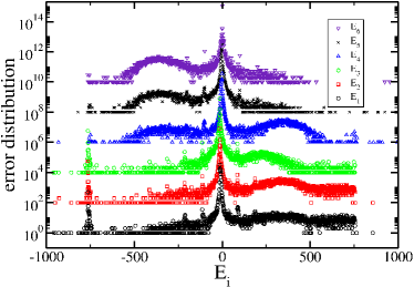
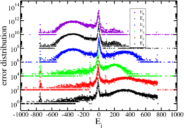
The six independent distributions are shown in Fig. 1 for the presidential process of July 2012. As can be seen there the whole behaviour is similar to that in the distributions calculated for the 2000 (see Fig. 2) and 2006 (Fig. 3) processes. As explained below they are the histograms of the number of cabins that have values of error equal to 0,1,2,. Certainly, it can be interpreted as appearance and missing of votes, but in fact it is a measure on how we count the electoral results. The errors can be intentional cheating or counting mistakes. For the present case some changes appeared in the labels of the dataset, for instance, the “Total number of Ballots deposited”, Bd, are now “Total number of extracted ballots from the urn”; the sum of all the votes for the different political parties and candidates is now made directly by the IFE’s computers. In the last case, we test the value calculated by the computers and the sum on the records with no main differences. It is important to notice that the final electoral results are presented and accounted after all the parties reached an agreement on the results in each polling station.
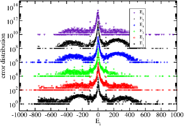
In all the figures the distributions are scaled by a factor of each time and in a log-linear graph in order to appreciate all of them in a single figure. In all the cases the central part has a power law decay and two asymmetrical lobes. Large peaks appear in all the graphs in Figs. 1 to 3. The reasons for this behaviour is unclear but it looks as a general feature that deserves a wide and detailed studyHernandezSaldana_IIbarra .
Prediction ii) The Partido Revolucionario Institucional (PRI) is a sprinter
Even when the behaviour presented here for the presidential candidates of the Partido Revolucionario Institucional appeared in election for the both chambers we shall concentrate in the presidential case. A graph of the percentage of votes for each party/candidate against the percentage of computed polling stations had been presented in voters outcome reports for federal elections in 2000 and 2006. In reference HernandezSaldanaE0 , version 3, both elections are reported. In Figure 1 and 2 of 2006, and in Figure 9 for 2000 the results are presented. In all the analyzed cases, the PRI showed a change in the percentage of votes’ slope. Close to the of computed polling stations an increase in the percentage of votes is evident. No matter that in both elections this party did not obtain the largest amount of votes, it appears ruling in polling stations arriving at the end of the counting process. It is a well known fact, due to historical reasons, that PRI receives a lot of votes in geographical regions with a high marginalization index(see for instance Pliego ), such regions are expected to have a slow electoral data processing and transmission to capture centers. This might explain why PRI is a sprinter. In HernandezSaldanaE4 the prediction was:
In the graph of percentage of vote against percentage of processed certificates the PRI will change its rate of growth around the time when of the computed certificates arrive. i.e. this political party has a good final sprint.
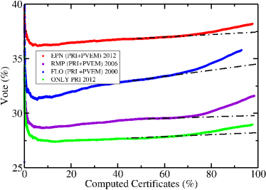
In order to test this prediction we report, in Figure 4, the percentage of vote obtained by PRI against the percentage of computed certificates of the polling stations. We report the presidential candidates in 2012 (EPN, Enrique Peña Nieto), 2006, (RMP, Roberto Madrazo Pintado) and, 2000 (FLO, Francisco Labastida Ochoa). For the July 2012 election the rules changed, candidates in coalitions appeared in the ballot in coalition and as candidate of one party. So, we can differentiate the votes for PRI only, from those obtained by the options PRI+PVEM and PVEM alone. Hence, we present the case for PRI alone as well. As can be observed in the Figure 4, for all of these cases the PRI changes its growth slope, increasing, in a noticeable way, the percentage of votes. No matter if we analyze PRI alone or the coalition. The change in slope is different in all the cases. The small party in a coalition presents a typical small party behaviour, (not shown). Hence, From Figure 4 it is clear that prediction ii) has been verified.
Some small details about Figure 4. All the polling stations certificates were considered in the figure, hence it has small fluctuations that are not appreciable due to the plotting character size. The present figure was processed in order to keep the file size small. The PREP record ends at a certain hour, usually 24-26 hours after the beginning of capture and does not include of the polling stations. So the end of records is different for each process.
Prediction iii) The PRI has a smooth vote distribution
Beyond the important discussion about universal features in vote distribution in world wide elections, a corporate political party has been extremely regular: the Partido Revolucionario Institucional (PRI). In all the previously performed analysis,HernandezSaldanaE0 ; HernandezSaldanaE1 ; HernandezSaldanaE2 ; HernandezSaldanaE3 its vote distribution is a smooth function. In reference HernandezSaldanaE1 , the smooth behaviour of this party in federal elections 2000, 2003 and 2006 using the definitive dataset of Count by District was reported. A similar behaviour has been observed in the 1997 and the 1994 elections by the author but the results remain unpublished.
The distribution of votes is the histogram of the number of polling stations with a certain amount of votes, properly scaled and normalized in order to have a normalized to unity distribution with a unit mean as well. In order to do the comparison with probability distribution the amount of votes is “unfolded” or “deconvoluted” by using the average of the number of votes, which scale properly the variable. The resulting histogram must be normalized to area one. (In reference HernandezSaldanaE2 there is an explanation, but this procedure is standard in data treatment.)
After this process, fitting a model is possible. Daisy functionsHernandezSaldana1999 , of different ranks, were tested with success for the 2000, 2003 and 2006 electoral processes for president and for both chambers. The only free parameter in this model is the rank, , and is written as:
| (1) |
With an integer and the Gamma function.
However, this distribution is a particular case of a more general distribution named the Gamma distribution. It is characterized by two real free parameters, and GammaDistributionCRC ; GammaDistributionMath and written as:
| (2) |
Here the free parameters are real numbers. When and we recover Eq. (1).
In this term, the third prediction was presented as:
The distribution of votes for PRI, in presidential and both chambers elections, fit smooth distributions, in general a Gamma distribution or Daisy models.
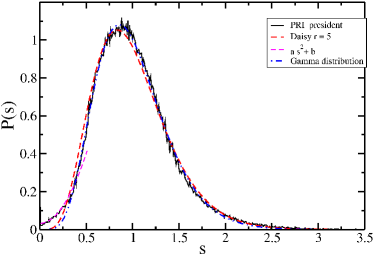
The result for the 2012 case is presented in Figure 5 and corresponds only to the presidential case for the votes for PRI alone. We left the other cases for a future work. There, the normalized histogram is presented in a black line. It is noticeable that the beginning of the distribution is not compatible with the fast decay at the tail and presents an abrupt change in slope (not shown). Such behaviour certainly can be analyzed with the Gamma distribution, but we keep the analysis apart since this kind of change in the slope has been reported for the 2003 intermediate elections. There, the behaviour corresponds to a different dynamic. The beginning of the distribution in Figure 5 is fitted by a quadratic polynomial with no linear term.
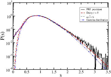
For the distribution remaining part we test our two models. In broken red line appears a Daisy model of rank which follows the curve nicely. The tail is clearly compatible with this Daisy as can be seen in Figure 6, where the same plot is presented but in log-linear scale in order to observe the exponential decay. Notice that the Daisy model runs inside the range of fluctuations. Other ranks of Daisy models do not fit the actual data.
In order to test how good the Daisy model is, we contrast it with the Gamma distribution with two free parameters, equation (2). The fit was obtained for different starting points, since the change in slope is at . For fittings starting beyond this point the results are around and . All the results are compatible with a Daisy model, since the relation between and remains as . Hence, prediction iii) was fulfilled, PRI has a smooth vote distribution described by Daisy models.
A detailed analysis of the exact values of the parameters is irrelevant at this moment since we do not have a theoretical model that explains this smooth behaviour. There are efforts in this way HernandezSaldanaE2 ; HernandezSaldanaE3 . Additionally, the results can be a mixture of dynamics since the histogram is built up using the complete database and does not consider differences in district or state, or if the state has been ruled by PRI for a long time. It is important to know that in several Mexican states PRI rules since 1929. The analysis of PRI’s distribution of votes performed by state and district is in progress.
Conclusions
Any scientific work must provide predictions, even when they could be based only on empirical observations. To have a valid theoretical framework for the regularities is a much more satisfactory result, but social systems are not well understood and this opens wide opportunities for research and for new multidisciplinary approaches.
In this paper I offer evidence that Mexican elections, as many others in several countries and years, present regularities. The first fulfilled prediction is of a general nature and it says that errors are always present, due to honest mistakes or to intentional cheating. Here we show that for the third time in a row, mexican elections show characteristic distributions of error in the self-consistency records. The reason for this behavior is unclear and deserves a separate analysis HernandezSaldana_IIbarra since they appeared in datasets that correspond to contrasting political environments: 1) lack of suspicion of fraud in presidential election (July 2000) with the defeat of the long time ruling party, 2) large suspicion of fraud (July 2006) and, 3) comeback to power of the ancient political party. Hence, this kind of behavior appeared in all of them. Certainly, local fraud by all political parties in Mexico is well documented, and we hope that some of the common practices appear under a much more detailed analysis.
The second succesful prediction is a result of history and geography: PRI has a well established promotional system that has ruled for many years. So, no magic intelligence needs to be invoked in order to explain this time domain behaviour. Wider studies could confirm this. The third accomplished prediction is a much more delicate question. The appearance of probability distributions in a process is, in general, evidence of some sort of general principle behind it. Such is the case of Gaussian distributions or power laws. The appearance of Daisy models in all of the PRI electoral process could open a door to understand corporative practices of parties around the world.
I Discussion
II Materials and Methods
All the used datasets are public via the web page of IFE IFEweb . Some dataset are available upon request through the IFE authorities infomex_ife or the author’s e-mail. The files in text format contain empty fields or comments, some of them are explicit in the annexed documentation. For simplicity I did not consider any polling station recorded with an empty field. The analysis of the error distribution of 2006 PREP was performed again with the data base of accepted polling station certificates. All the data treament was made in fortran 77 and the source code is available from the author.
Acknowledgments
This work was supported by PROMEP/SEP and CONACyT. I thank to E. Várguez for encouragement and support. The author acknowledges the hospitality of the Auberge Várguez-Villanueva where this work was ended.
References
- (1) Castellano C, Fortunato S, Loreto V (2009) Statistical physics of social dynamics. Rev Mod Phys 81: 591-646.
- (2) Fortunato S, Castellano C (2007) Scaling and universality in proportional elections. Phys Rev Lett 99: 138701.
- (3) Costa Filho RN, Almeida MP, Andrade JS, Moreira JE (1999) Scaling behavior in a proportional voting process. Phys Rev E 60: 1067–1068.
- (4) Costa Filho RN, Almeida M, Moreira J, Andrade Jr J (2003) Brazilian elections: voting for a scaling democracy. Physica A 322: 698 - 700.
- (5) Araripe LE, Costa Filho RN (2009) Role of parties in the vote distribution of proportional elections. Physica A 388: 4167-4170.
- (6) Araripe LE, Costa Filho RN, Herrmann HJ, Andrade Jr JS (2006) Plurality voting: The statistical laws of democracy in Brazil. Int J Mod Phys C 17: 1809-1813.
- (7) Hernández-Saldaña H (2009) On the corporate votes and their relation with daisy models. Physica A 388: 2699-2704.
- (8) Borghesi C, Raynal JC, Bouchaud JP (2012) Election Turnout Statistics in Many Countries: Similarities, Differences, and a Diffusive Field Model for Decision-Making. PLoS ONE 7.
- (9) Borghesi C, Chiche J, Nadal JP (2012) Between Order and Disorder: A ‘Weak Law’ on Recent Electoral Behavior among Urban Voters? PLoS ONE 7.
- (10) Chatterjee A, Mitrović M, Fortunato S (2013) Universality in voting behavior: an empirical analysis. Scientific Reports - Nature 3: 1049.
- (11) Borghesi C (2009). Three quantitative predictions based on past regularities about voter turnout at the french 2009 european election. ArXiv:0905.4578v1 [physics.soc-ph].
- (12) Borghesi C (2009). Results of three quantitative predictions based on past regularities about voter turnout at the french 2009 european election. ArXiv:0906.2692v1 [physics.soc-ph].
- (13) Hernández-Saldaña H (2012) Three predictions on july 2012 federal elections in mexico based on past regularities. arXiv:1207.0078 [physics.soc-ph].
- (14) http://www.ife.org.mx, http://prep2012.ife.org.mx.
- (15) http://www.ife.org.mx/informacion-relevante.html.
- (16) Klesner J (2007) The july 2006 presidential and congressional elections in mexico. Electoral Studies 26: 803-808.
-
(17)
https://ciudadania.ife.org.mx/infomex
/ActionInitSAILoginINFOMEX.do. - (18) Hernández-Saldaña H (2010) Travelling Salesman Problem, Theory and Applications, InTech, chapter 16. pp. 283-298.
- (19) Báez G, Hernández-Saldaña H, Méndez-Sánchez R (2006) On the reliability of voting processes: the mexican case. arXiv:physics/0609144 versions 1, 2 and 3.
- (20) Ibarra I, Hernández-Saldaña H. Work in progress.
- (21) Pliego Carrasco F (2007) El mito del fraude electoral en México, Pax, México. p. 218.
- (22) Hernández-Saldaña H, Gómez Quesada M, Hernández-Zapata E (2012) Statistical distributions of quasi-optimal paths in the traveling salesman problem: The role of initial distribution of cities. Rev Mex Fís S 58: 0032.
- (23) Hernández-Saldaña H, Flores J, Seligman T (1999) Semi-Poisson statistics and beyond. Phys Rev E 60: 449-452.
- (24) Beyer WH (1987) CRC Standard Mathematical Tables. Boca Raton, FL: CRC Press, 28th edition, 534 pp.
- (25) Weisstein EW. Gamma distribution. From MathWorld–A Wolfram Web Resource. http://mathworld.wolfram.com/GammaDistribution.html.