Sparse Hopfield network reconstruction with $\ell_{1}$ regularization

Abstract

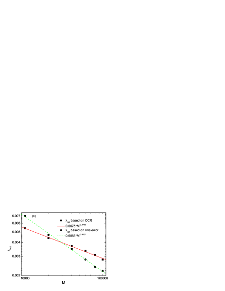
We propose an efficient strategy to infer sparse Hopfield network based on magnetizations and pairwise correlations measured through Glauber samplings. This strategy incorporates the $\ell_{1}$ regularization into the Bethe approximation by a quadratic approximation to the log-likelihood, and is able to further reduce the inference error of the Bethe approximation without the regularization. The optimal regularization parameter is observed to be of the order of $M^{-\nu}$ where $M$ is the number of independent samples. The value of the scaling exponent depends on the performance measure. $\nu\simeq 0.5001$ for root mean squared error measure while $\nu\simeq 0.2743$ for misclassification rate measure. The efficiency of this strategy is demonstrated for the sparse Hopfield model, but the method is generally applicable to other diluted mean field models. In particular, it is simple in implementation without heavy computational cost.

I Introduction

The inverse Ising problem is intensively studied in statistical physics, computational biology and computer science in the few past years Schneidman et al. (2006); Cocco et al. (2009); Morcos et al. (2011); Ravikumar et al. (2010). The biological experiments or numerical simulations usually generate a large amount of experimental data, e.g., $M$ independent samples $\{\boldsymbol{\sigma}^{1},\boldsymbol{\sigma}^{2},\ldots,\boldsymbol{\sigma}^{M}\}$ in which $\boldsymbol{\sigma}$ is an $N$-dimensional vector with binary components ($\sigma_{i}=\pm 1$) and $N$ is the system size. The least structured model to match the statistics of the experimental data is the Ising model Tkacik et al. (2009):

$$P_{{\rm Ising}}(\boldsymbol{\sigma})=\frac{1}{Z(\mathbf{h},\mathbf{J})}\exp\left[\sum_{i<j}J_{ij}\sigma_{i}\sigma_{j}+\sum_{i}h_{i}\sigma_{i}\right]$$ (1)

where the partition function $Z(\mathbf{h},\mathbf{J})$ depends on the $N$-dimensional fields and $\frac{N(N-1)}{2}$-dimensional couplings. These fields and couplings are chosen to yield the same first and second moments (magnetizations and pairwise correlations respectively) as those obtained from the experimental data. The inverse temperature $\beta=1/T$ has been absorbed into the strength of fields and couplings.

Previous studies of the inverse Ising problem on Hopfield model Huang (2010a, b); Cocco et al. (2011); Braunstein et al. (2011); Huang (2012) lack a systematic analysis for treating sparse networks. Inference of the sparse network also have important and wide applications in modeling vast amounts of biological data. Actually, the real biological network is not densely connected. To reconstruct the sparse network from the experimental data, an additional penalty term is necessary to be added into the cost function, as studied in recovering sparse signals in the context of compressed sensing Kabashima et al. (2009); Bayati et al. (2010); Zibulevsky and Elad (2010) or in Ising model selection Ravikumar et al. (2010); Bento and Montanari (2011). This strategy is known as $\ell_{1}$-regularization which introduces an $\ell_{1}$-norm penalty to the cost function (e.g., the log-likelihood of the Ising model). The regularization is able to minimize the impact of finite sampling noise, thus avoid the overfitting of data. The $\ell_{1}$-regularization has been studied in the pseudo-likelihood approximation to the network inference problemAurell and Ekeberg (2012) and in the setting of sparse continuous perceptron memorization and generalization Lage-Castellanos et al. (2009). This technique has also been thoroughly discussed in real neural data analysis using selective cluster expansion method Barton and Cocco (2013); Cocco and Monasson (2012). The cluster expansion method involves repeated solution of the inverse Ising problem and the computation of the cluster entropy included in the expansion (cluster means a small subset of spins). To truncate the expansion, clusters with small entropy in absolute value are discarded and the optimal threshold needs to be determined. Additionally, the cluster size should be small to reduce the computational cost while at each step a convex optimization of the cost function (see Eq. (9)) for the cluster should be solved. This may be complicated in some cases. The pseudo-likelihood maximization Aurell and Ekeberg (2012) method relies on the complete knowledge of the sampled configurations, and involves a careful design of the numerical minimization procedure for the pseudo-likelihood (e.g., Newton descent method, or interior point method) at a large computational cost (especially for large sample size). In this paper, we provide an alternative way to reconstruct the sparse network by combining the Bethe approximation and the $\ell_{1}$-regularization, which is much simpler in practical implementation. We expect that the $\ell_{1}$-regularization will improve the prediction of the Bethe approximation. To show the efficiency, we apply this method to the sparse Hopfield network reconstruction.

Our contributions in this work are two-fold. (1) We provide a regularized quadratic approximation to the negative log-likelihood function for the sparse network construction by neglecting higher order correlations, which yields a new inference equation reducing further the inference error. Furthermore, the implementation is much simple by saving the computational time. (2) Another significant contribution is a scaling form for the optimal regularization parameter is found, and this scaling form is useful for choosing the suitable regularization. Most importantly, the method is not limited to the tested model (sparse Hopfield model), and is generally applicable to other diluted mean field models and even real data analysis (e.g., neural data). The outline of the paper is as follows. The sparse Hopfield network is defined in Sec. II. In Sec. III, we present the hybrid inference method by using the Bethe approximation and $\ell_{1}$-regularization. We test our algorithm on single instances in Sec. IV. Concluding remarks are given in Sec. V.

II Sparse Hopfield model

The Hopfield network has been proposed in Ref. Hopfield (1982) as an abstraction of biological memory storage and was found to be able to store an extensive number of random unbiased patterns Amit et al. (1987). If the stored patterns are dynamically stable, then the network is able to provide associative memory and its equilibrium behavior is described by the following Hamiltonian:

$$\mathcal{H}=-\sum_{i<j}J_{ij}\sigma_{i}\sigma_{j}$$ (2)

where the Ising variable $\sigma$ indicates the active state of the neuron ($\sigma_{i}=+1$) or the silent state ($\sigma_{i}=-1$). For the sparse network storing $P$ random unbiased binary patterns, the symmetric coupling is constructed Sompolinsky (1986); Okada et al. (1998) as

$$J_{ij}=\frac{l_{ij}}{l}\sum_{\mu=1}^{P}\xi_{i}^{\mu}\xi_{j}^{\mu}$$ (3)

where $l$ is the average connectivity of the neuron. $l\sim\mathcal{O}(1)$ independent of the network size $N$. Note that in this case, the number of stored patterns can only be finite. In the thermodynamic limit, $P$ scales as $P=\alpha l$ where $\alpha$ is the memory load. No self-interactions are assumed and the connectivity $l_{ij}$ obeys the distribution:

$$P(l_{ij})=\left(1-\frac{l}{N-1}\right)\delta(l_{ij})+\frac{l}{N-1}\delta(l_{ij}-1).$$ (4)

Mean field properties of the sparse Hopfield network have been discussed within replica symmetric approximation in Refs. Wemmenhove and Coolen (2003); Castillo and Skantzos (2004). Three phases (paramagnetic, retrieval and spin glass phases) have been observed in this sparsely connected Hopfield network with arbitrary finite $l$. For large $l$ (e.g., $l=10$), the phase diagram resembles closely that of extremely diluted ($\lim_{N\rightarrow\infty}l^{-1}=\lim_{N\rightarrow\infty}l/N=0$, such as $l=\ln N$) case Watkin and Sherrington (1991); Canning and Naef (1992) where the transition line between paramagnetic and retrieval phase is $T=1$ for $\alpha\leq 1$ and that between paramagnetic and spin glass phase $T=\sqrt{\alpha}$ for $\alpha\geq 1$. The spin glass/retrieval transition occurs at $\alpha=1$.

To sample the state of the original model Eq. (2), we apply the Glauber dynamics rule:

$$P(\sigma_{i}\rightarrow-\sigma_{i})=\frac{1}{2}\left[1-\sigma_{i}\tanh\beta h_{i}\right]$$ (5)

where $h_{i}=\sum_{j\neq i}J_{ij}\sigma_{j}$ is the local field neuron $i$ feels. In practice, we first randomly generate a configuration which is then updated by the local dynamics rule Eq. (5) in a randomly asynchronous fashion. In this setting, we define a Glauber dynamics step as $N$ proposed flips. The Glauber dynamics is run totally $3\times 10^{6}$ steps, among which the first $1\times 10^{6}$ steps are run for thermal equilibration and the other $2\times 10^{6}$ steps for computing magnetizations and correlations, i.e., ${m_{i}=\left<\sigma_{i}\right>_{{\rm data}},C_{ij}=\left<\sigma_{i}\sigma_{j}\right>_{{\rm data}}-m_{i}m_{j}}$ where $\left<\cdots\right>_{{\rm data}}$ denotes the average over the collected data. The state of the network is sampled every $20$ steps after thermal equilibration (doubled sampling frequency yields the similar inference result), which produces totally $M=100000$ independent samples. The magnetizations and correlations serve as inputs to our following hybrid inference algorithm.

III Bethe approximation with $\ell_{1}$ regularization

The Bethe approximation assumes that the joint probability (Boltzmann distribution, see Eq. (1)) of the neuron activity can be written in terms of single-neuron marginal for each single neuron and two-neuron marginal for each pair of adjacent neurons as

$$P_{{\rm Ising}}(\boldsymbol{\sigma})\simeq\prod_{(ij)}\frac{P_{ij}(\sigma_{i},\sigma_{j})}{P_{i}(\sigma_{i})P_{j}(\sigma_{j})}\prod_{i}P_{i}(\sigma_{i})$$ (6)

where $(ij)$ runs over all distinct pairs of neurons. This approximation is exact on tree graphs and asymptotically correct for sparse networks or networks with sufficiently weak interactions Mézard and Mora (2009). Under this approximation, the free energy ($-\ln Z$) can be expressed as a function of connected correlations $\{C_{ij}\}$ (between neighboring neurons) and magnetizations $\{m_{i}\}$. The stationary point of the free energy with respect to the magnetizations yields the following self-consistent equations:

$$m_{i}=\tanh\left(h_{i}+\sum_{j\in\partial i}\tanh^{-1}\left(t_{ij}f(m_{j},m_{i},t_{ij})\right)\right)$$ (7)

where $\partial i$ denotes neighbors of $i$, $t_{ij}=\tanh J_{ij}$ and $f(x,y,t)=\frac{1-t^{2}-\sqrt{(1-t^{2})^{2}-4t(x-yt)(y-xt)}}{2t(y-xt)}$. Using the linear response relation to calculate the connected correlations for any pairs of neurons, we obtain the Bethe approximation (BA) to the inverse Ising problem Ricci-Tersenghi (2012); Nguyen and Berg (2012):

$$J_{ij}=-\tanh^{-1}\Biggl{[}\frac{1}{2(\mathbf{C}^{-1})_{ij}}(a_{ij}-b_{ij})-m_{i}m_{j}\Biggr{]},$$ (8)

where $\mathbf{C}^{-1}$ is the inverse of the connected correlation matrix, $a_{ij}=\sqrt{1+4L_{i}L_{j}(\mathbf{C}^{-1})_{ij}^{2}}$, $L_{i}=1-m_{i}^{2}$ and $b_{ij}=\sqrt{\left(a_{ij}-2m_{i}m_{j}(\mathbf{C}^{-1})_{ij}\right)^{2}-4(\mathbf{C}^{-1})_{ij}^{2}}$. The couplings have been scaled by the inverse temperature $\beta$. Note that fields can be predicted using Eq. (7) after we get the set of couplings. Hereafter we consider only the reconstruction of the coupling vector. In fact, the BA solution of the couplings corresponds to the fixed point of the susceptibility propagation Mézard and Mora (2009); Huang (2010b), yet it avoids the iteration steps in susceptibility propagation and the possible non-convergence of the iterations. It was also found that the BA yields a good estimate to the underlying couplings of the Hopfield network Huang (2010b). In the following analysis, we try to improve the prediction of BA with $\ell_{1}$-regularization.

The cost function to be minimized in the inverse Ising problem can be written as the following rescaled negative log-likelihood function Sessak and Monasson (2009):

$$\begin{split}S(\mathbf{h},\mathbf{J}|\mathbf{m},\mathbf{C})&=-\frac{1}{M}\ln\left[\prod_{\mu=1}^{M}P_{{\rm Ising}}(\boldsymbol{\sigma}^{\mu}|\mathbf{h},\mathbf{J})\right]\\ &=\ln Z(\mathbf{h},\mathbf{J})-\mathbf{h}^{T}\mathbf{m}-\frac{1}{2}{\rm tr}(\mathbf{J}\mathbf{\tilde{C}})\end{split}$$ (9)

where $m_{i}=\left<\sigma_{i}\right>_{{\rm data}}$ and $\tilde{C}_{ij}=\left<\sigma_{i}\sigma_{j}\right>_{{\rm data}}$. $\mathbf{h}^{T}$ denotes the transpose of the field vector while ${\rm tr}(\mathbf{A})$ denotes the trace of matrix $\mathbf{A}$. The minimization of $S(\mathbf{h},\mathbf{J}|\mathbf{m},\mathbf{C})$ in the $\frac{N(N+1)}{2}$-dimensional space of fields and couplings yields the following equations:

$$m_{i} =\left<\sigma_{i}\right>,$$ (10a)

$$C_{ij} =\left<\sigma_{i}\sigma_{j}\right>-\left<\sigma_{i}\right>\left<\sigma_{j}\right>$$ (10b)

where the average is taken with respect to the Boltzmann distribution Eq. (1) with the optimal fields and couplings (corresponding to the minimum of $S$). Actually, one can use Bethe approximation to compute the connected correlation in the right-hand side of Eq. (10b), which leads to the result of Eq. (8).

To proceed, we expand the cost function around its minimum with respect to the fluctuation of the coupling vector up to the second order as

$$S(\mathbf{J})\simeq S(\mathbf{J}_{0})+\nabla S(\mathbf{J}_{0})^{T}\mathbf{\tilde{J}}+\frac{1}{2}\mathbf{\tilde{J}}^{T}\mathbf{H}_{S}(\mathbf{J}_{0})\mathbf{\tilde{J}}$$ (11)

where $\mathbf{\tilde{J}}$ defines the fluctuation $\mathbf{\tilde{J}}\equiv\mathbf{J}-\mathbf{J}_{0}$ where $\mathbf{J}_{0}$ is the (near) optimal coupling vector. $\nabla S(\mathbf{J}_{0})$ is the gradient of $S$ evaluated at $\mathbf{J}_{0}$, and $\mathbf{H}_{S}(\mathbf{J}_{0})$ is the Hessian matrix. The quadratic approximation to the log-likelihood has also been used to develop fast algorithms for estimation of generalized linear models with convex penalties Friedman et al. (2010). We have only made explicit the dependence of $S$ on the coupling vector. The first order coefficient vanishes due to Eq. (10). Note that the Hessian matrix is an $N(N-1)/2\times N(N-1)/2$ symmetric matrix whose dimension is much higher than that of the connected correlation matrix. However, to construct the couplings around neuron $i$, we consider only the neuron $i$-dependent part, i.e., we set $l=i$ in the Hessian matrix $\chi_{ij,kl}=\left<\sigma_{i}\sigma_{j}\sigma_{k}\sigma_{l}\right>-\left<\sigma_{i}\sigma_{j}\right>\left<\sigma_{k}\sigma_{l}\right>$ where $ij$ and $kl$ run over distinct pairs of neurons. This simplification reduces the computation cost but still keeps the significant contribution as proved later in our simulations. Finally we obtain

$$S(\mathbf{J})\simeq S(\mathbf{J}_{0})+\frac{1}{2}\sum_{ij,ki}\tilde{J}_{ij}(\tilde{C}_{jk}-\tilde{C}_{ij}\tilde{C}_{ki})\tilde{J}_{ki}+\lambda\sum_{ij}|J_{0,ij}+\tilde{J}_{ij}|$$ (12)

where an $\ell_{1}$-norm penalty has been added to promote the selection of sparse network structure Hertz et al. (2011); Barton and Cocco (2013); Bento and Montanari (2011). $\lambda$ is a positive regularization parameter to be optimized to make the inference error (see Eq. (14)) as low as possible. The $\ell_{1}$-norm penalizes small but non-zero couplings and increasing the value of the regularization parameter $\lambda$ makes the inferred network sparser. In the following analysis, we assume $\mathbf{J}_{0}$ is provided by the BA solution (a good approximation to reconstruct the sparse Hopfield network Huang (2010b), yielding a low inference error), then we search for the new solution to minimize the regularized cost function Eq. (12), finally we get the new solution as follows,

$$J^{(i)}_{ij}=J_{0,ij}-\lambda\sum_{k}{\rm sgn}(J_{0,ik})[\mathbf{C}^{i}]^{-1}_{kj}$$ (13)

where ${\rm sgn}(x)=x/|x|$ for $x\neq 0$ and $(\mathbf{C}^{i})_{kj}=\tilde{C}_{kj}-\tilde{C}_{ji}\tilde{C}_{ik}$. Eq. (13) results from $\frac{\partial S(\mathbf{J})}{\partial J_{ij}}=0$ which gives $\mathbf{\tilde{J}}^{T}\mathbf{C}^{i}=\boldsymbol{\Lambda}^{T}$, where $\Lambda_{j}=-\lambda{\rm sgn}(J_{0,ij})(j\neq i)$ and $\tilde{J}_{j}=J_{ij}-J_{0,ij}(j\neq i)$. $J^{(i)}_{ij}$ represents couplings around neuron $i$. To ensure the symmetry of the couplings, we construct $J_{ij}=\frac{1}{2}(J^{(i)}_{ij}+J^{(j)}_{ji})$ where $J^{(j)}_{ji}$ is also given by Eq. (13) in which $i$ and $j$ are exchanged. The inverse of $\mathbf{C}^{i}$ or $\mathbf{C}^{j}$ takes the computation time of the order $\mathcal{O}(N^{3})$, much smaller than that of the inverse of a susceptibility matrix $\boldsymbol{\chi}$.

We remark here that minimizing the regularized cost function Eq. (12) corresponds to finding the optimal deviation $\mathbf{\tilde{J}}$ which provides a solution to the regularized cost function. We also assume that for small $\lambda$, the deviation is small as well. Without the quadratic approximation in Eq. (11), no closed form solution exists for the optimal $\mathbf{J}$, however, the solution can still be found by using convex optimization techniques. Similar equation to Eq. (13) has been derived in the context of reconstructing a sparse asymmetric, asynchronous Ising network Zeng et al. (2012). Here we derive the inference equation (Eq. (13)) for the static reconstruction of a sparse network. We will show in the next section the efficiency of this hybrid strategy to improve the prediction of the BA without regularization. To evaluate the efficiency, we define the reconstruction error (root mean squared (rms) error) as

$$\Delta_{J}=\left[\frac{2}{N(N-1)}\sum_{i<j}(J_{ij}^{*}-J_{ij}^{{\rm true}})^{2}\right]^{1/2}$$ (14)

where $J_{ij}^{*}$ is the inferred coupling while $J_{ij}^{{\rm true}}$ is the true one constructed according to Eq. (3). Other performance measures for sparse network inference will also be discussed in the following section.

IV Results and discussions

Figure 1: (Color online) (a) Improvement of the prediction by $\ell_{1}$-regularized BA on sparse Hopfield networks. The inference error by BA with prior knowledge of the sparseness of the network is also shown. Network size $N=100$, the memory load $\alpha=0.6$ and the mean node degree $l=5$. Each data point is the average over five random sparse networks. The regularization parameter has been optimized. The inset gives the relative inference error defined as $\frac{\Delta_{J}^{BA}-\Delta_{J}^{reg}}{\Delta_{J}^{BA}}$ versus the inverse temperature. (b) The receiver operating characteristic curve for three typical examples ($T=1.4$). Each data point corresponds to a value of $\lambda$ for $\ell_{1}$-regularized BA. The solid symbol gives the result of BA without regularization. Parameters for these three examples are $(N,P,\alpha)=(40,3,0.6),(100,3,0.6),(100,5,1.2)$ respectively.

Figure 2: (Color online) (a) Reconstruction error $\Delta_{J}$ versus the regularization parameter $\lambda$ at $T=1.4$. Inference results on three random instances are shown. The inference errors by applying BA without regularization on these three random instances are $\Delta_{J}=0.006108,0.006049,0.005981$ respectively. (b) Correct classification rate (CCR) versus the regularization parameter $\lambda$ at $T=1.4$. The instances are the same as those in (a). The CCR of BA without regularization are ${\rm CCR}=0.9224,0.9178,0.9162$ respectively. (c) The optimal $\lambda_{{\rm opt}}$ versus the number of samples $M$ ($T=1.4$). Each point is the mean value over five random realizations of the sparse Hopfield network. The standard error is nearly zero and not shown. The linear fit shows that $\lambda_{{\rm opt}}=\lambda_{0}M^{-\nu}$ with $\lambda_{0}\simeq 0.6883,\nu\simeq 0.5001$ for rms error and $\lambda_{0}\simeq 0.0675,\nu\simeq 0.2743$ for CCR measure.

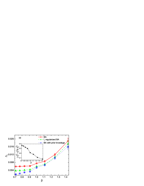
We simulate the sparsely connected Hopfield network of size $N=100$ at different temperatures. The average connectivity for each neuron $l=5$ and the memory load $\alpha=0.6$. As shown in fig. 1 (a), the $\ell_{1}$-regularization in Eq. (13) does improve the prediction on the sparse network reconstruction. The improvement is evident in the presence of high quality data (e.g., in the high temperature region, see the inset of fig. 1 (a)). However, the relative inference error (improvement fraction) shown in the inset of fig. 1 (a) gets smaller as the temperature decreases. This may be due to insufficient samplings Huang (2012) of glassy states at the low temperatures. The glassy phase is typically characterized by a complex energy landscape exhibiting numerous local minima. As a result, the phase space we sample develops higher order (higher than second order) correlations whose contributions to the regularized cost function can not be simply neglected, which explains the behavior observed in the inset of fig. 1 (a). In this case, the pseudo-likelihood method or more complex selective cluster expansion can be used at the expense of larger computation times. For comparison, we also show the inference error of BA with prior knowledge of the network connectivity, i.e., the sparseness is known in advance with only the true non-zero couplings to be predicted. The comparison confirms that the $\mathbf{C}^{i}$ matrix obtained from correlations in the data contains useful information about the sparsity of the network, and this information can be extracted by using $\ell_{1}$-regularization in Eq. (13).

An accurate pruning of the network can be achieved by simple thresholding (setting to zero some couplings whose absolute values are below certain threshold) based on the improved prediction. The receiver operating characteristic (ROC) curves are given in fig. 1 (b) for three typical examples of different network size, memory load and connectivity. The ROC curve is obtained by plotting true positive rate (the number of inferred non-zero couplings with correct sign divided by the total number of true non-zero couplings) against true negative rate (the number of inferred zero couplings divided by the total number of true zero couplings). A threshold $\delta=0.01$ is used to get the inferred zero couplings. The ROC curve in fig. 1 (b) shows that one can push the inference accuracy towards the upper right corner (high true positive rate as well as high true negative rate) by tuning the regularization parameter. Note that BA without regularization reports low true negative rate.

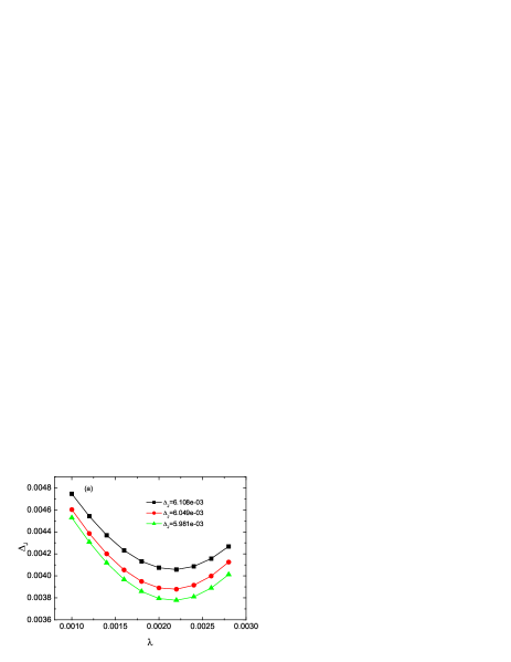
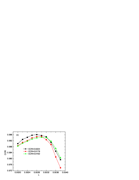
We also explore the effects of the regularization parameter on the reconstruction, which are reported in fig. 2 (a). With increasing $\lambda$, the inference error first decreases, then reaches a minimal value followed by an increasing trend in the range we plot in fig. 2 (a). This implies that the optimal regularization parameter guides our inference procedure to a sparse network closest to the original one. The inference quality can also be measured by the fraction of edges $(ij)$ where the coupling strength is classified correctly as ‘positive’, ‘zero’or ‘negative’. We call this quantity correct classification rate (CCR). Results for three typical examples are reported in fig. 2 (b). With increasing $\lambda$, CCR first increases and then decreases. The optimal regularization parameter corresponding to the maximum is slightly different from that in fig. 2 (a). By using regularized BA (Eq. (13)), one can achieve a much higher value of CCR, and furthermore the computational cost is not heavy. Interestingly, the optimal value of $\lambda$ yielding the lowest inference error (rms error) has the order of $\mathcal{O}(\sqrt{\frac{1}{M}})$ for fixed network size (usually $M\gg N$), which is consistent with that found in Refs. Ravikumar et al. (2010); Bento and Montanari (2011). We verify this scaling form by varying $M$ and plotting the optimal $\lambda$ in fig. 2 (c). The linear fit implies that the scaling exponent $\nu\simeq 0.5$. However, this scaling exponent depends on the performance measure. Taking the CCR measure yields a smaller value $\nu\simeq 0.2743$, as shown in fig. 2 (c) as well. We also find that the magnitude of the optimal regularization parameter shows less sensitivity to specific instances and other parameters (e.g., the temperature, memory load or network size), since the number of samplings $M$ dominates the order of the magnitude. The specific optimal value becomes slightly different across different instances of the sparse network in the low temperature region, where its mean value shifts to a bit larger value for rms error measure or a bit smaller value for CCR measure, as the temperature further decreases. The number of samplings $M$ determines the order of the magnitude, which helps us find the appropriate strength for the regularization parameter. In the real application, the true coupling vector is a priori unknown. In this case, the regularization parameter can be chosen to make the difference between the measured moments and those produced by the reconstructed Ising model as small as possible.

Figure 3: (Color online) Comparison of performance measured by misclassification rate. Each data point is the average over five random sparse networks. The regularization parameter has been optimized. (a) Misclassification rate versus inverse temperature. Network size $N=100$, the memory load $\alpha=0.6$ and the mean node degree $l=5$. (b) Misclassification rate versus memory load. Network size $N=100$, temperature $T=1.4$ and $P=5$.

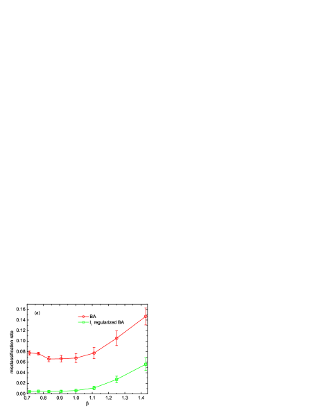
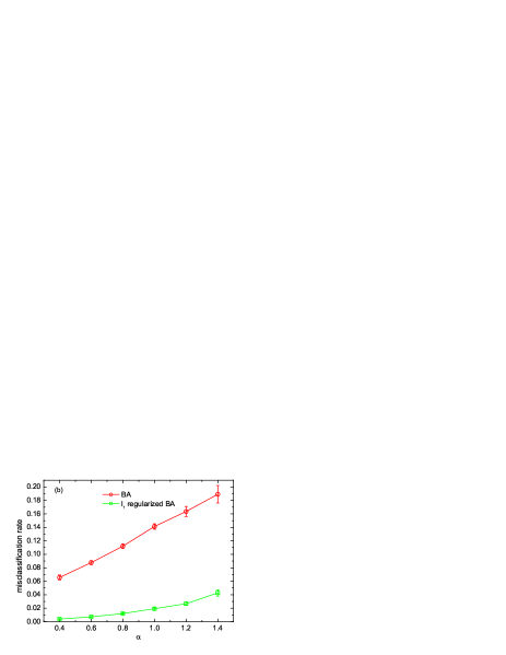
Finally, we give the comparison of performance measured by misclassification rate in fig. 3. According to the above definition, misclassification rate equals to $1-{\rm CCR}$. Low misclassification rate is preferred in the sparse network inference. Fig. 3 (a) shows the performance versus inverse temperature. The misclassification rate is lowered by a substantial amount using the hybrid strategy. Especially in the high temperature region, the error approaches zero while BA still yields an error of the order of $\mathcal{O}(10^{-2})$. As displayed in fig. 3 (b), the hybrid strategy is also superior to BA when the memory load is varied, although the misclassification rate grows with the memory load. Compared with BA, the $\ell_{1}$-regularized BA yields a much slower growth of the error when $\alpha$ increases. Even at the high memory load $\alpha=1.4$, the hybrid strategy is able to reconstruct the network with an error $4.3\%$ while at the same memory load, the error of BA is as large as $18.9\%$. Note that as $\alpha$ changes, the average connectivity also changes. Fig. 3 (b) illustrates that our simple inference strategy is also robust to different mean node degrees.

V Conclusion

We propose an efficient hybrid inference strategy for reconstructing the sparse Hopfield network. This strategy combines Bethe approximation and the $\ell_{1}$-regularization by expanding the objective function (negative log-likelihood function) up to the second order of the coupling fluctuation around its (near) optimal value. The hybrid strategy is simple in implementation without heavy computational cost, yet improves the prediction by zeroing couplings which are actually not present in the network (see fig. 1 and fig. 3). We can control the accuracy by tuning the regularization parameters. The magnitude of the optimal regularization parameters is determined by the number of independent samples $M$ as $\lambda_{{\rm opt}}\sim M^{-\nu}$. The value of the scaling exponent depends on the performance measure. $\nu\simeq 0.5$ for root mean squared error measure while $\nu\simeq 0.2743$ for misclassification rate measure. By varying the value of the regularization parameter, we show that the reconstruction (rms) error first decreases and then increases after the lowest error is reached. Similar phenomenon is observed for the change of misclassification rate with the regularization parameter. We observe this phenomenon in the sparse Hopfield network reconstruction, and this behavior may be different in other cases Barton and Cocco (2013). The efficiency of this strategy is demonstrated for the sparse Hopfield model, but this approximated reconstruction method is generally applicable to other diluted mean field models if we can first find a good solution (yielding low inference error) to the inverse Ising problem without regularization.

References

- Schneidman et al. (2006) E. Schneidman, M. J. Berry, R. Segev, and W. Bialek, Nature 440, 1007 (2006).
- Cocco et al. (2009) S. Cocco, S. Leibler, and R. Monasson, Proc. Natl. Acad. Sci. USA 106, 14058 (2009).
- Morcos et al. (2011) F. Morcos, A. Pagnani, B. Lunt, A. Bertolino, D. S. Marks, C. Sander, R. Zecchina, J. N. Onuchic, T. Hwa, and M. Weigt, Proc. Natl. Acad. Sci. USA 108, E1293 (2011).
- Ravikumar et al. (2010) P. Ravikumar, M. J. Wainwright, and J. D. Lafferty, Ann. Stat. 38, 1287 (2010).
- Tkacik et al. (2009) G. Tkacik, E. Schneidman, M. J. Berry, and W. Bialek (2009), e-print arXiv:0912.5409.
- Huang (2010a) H. Huang, Phys. Rev. E 81, 036104 (2010a).
- Huang (2010b) H. Huang, Phys. Rev. E 82, 056111 (2010b).
- Cocco et al. (2011) S. Cocco, R. Monasson, and V. Sessak, Phys. Rev. E 83, 051123 (2011).
- Braunstein et al. (2011) A. Braunstein, A. Ramezanpour, R. Zecchina, and P. Zhang, Phys. Rev. E 83, 056114 (2011).
- Huang (2012) H. Huang, Commun. Theor. Phys 57, 169 (2012).
- Kabashima et al. (2009) Y. Kabashima, T. Wadayama, and T. Tanaka, J. Stat. Mech.: Theory Exp p. L09003 (2009).
- Bayati et al. (2010) M. Bayati, J. Bento, and A. Montanari, in Neural. Inf. Process. Syst. (NIPS) (2010).
- Zibulevsky and Elad (2010) M. Zibulevsky and M. Elad, IEEE Signal Processing Magazine 27, 76 (2010).
- Bento and Montanari (2011) J. Bento and A. Montanari (2011), arXiv:1110.1769.
- Aurell and Ekeberg (2012) E. Aurell and M. Ekeberg, Phys. Rev. Lett 108, 090201 (2012).
- Lage-Castellanos et al. (2009) A. Lage-Castellanos, A. Pagnani, M. Weigt, and R. Zecchina, J. Stat. Mech.: Theory Exp p. P10009 (2009).
- Barton and Cocco (2013) J. Barton and S. Cocco, J. Stat. Mech.: Theory Exp p. P03002 (2013).
- Cocco and Monasson (2012) S. Cocco and R. Monasson, J. Stat. Phys 147, 252 (2012).
- Hopfield (1982) J. J. Hopfield, Proc. Natl. Acad. Sci. USA 79, 2554 (1982).
- Amit et al. (1987) D. J. Amit, H. Gutfreund, and H. Sompolinsky, Ann. Phys. 173, 30 (1987).
- Sompolinsky (1986) H. Sompolinsky, Phys. Rev. A 34, 2571 (1986).
- Okada et al. (1998) M. Okada, T. Fukai, and M. Shiino, Phys. Rev. E 57, 2095 (1998).
- Wemmenhove and Coolen (2003) B. Wemmenhove and A. C. C. Coolen, J. Phys. A 36, 9617 (2003).
- Castillo and Skantzos (2004) I. P. Castillo and N. S. Skantzos, J. Phys. A 37, 9087 (2004).
- Watkin and Sherrington (1991) T. L. H. Watkin and D. Sherrington, Europhys. Lett 14, 791 (1991).
- Canning and Naef (1992) A. Canning and J. P. Naef, J. Physique I 2, 1791 (1992).
- Mézard and Mora (2009) M. Mézard and T. Mora, J. Physiology Paris 103, 107 (2009).
- Ricci-Tersenghi (2012) F. Ricci-Tersenghi, J. Stat. Mech p. P08015 (2012).
- Nguyen and Berg (2012) H. C. Nguyen and J. Berg, J. Stat. Mech p. P03004 (2012).
- Sessak and Monasson (2009) V. Sessak and R. Monasson, J. Phys. A 42, 055001 (2009).
- Friedman et al. (2010) J. Friedman, T. Hastie, and R. Tibshirani, Journal of Statistical Software 33, 1 (2010).
- Hertz et al. (2011) J. Hertz, Y. Roudi, and J. Tyrcha (2011), e-print arXiv:1106.1752.
- Zeng et al. (2012) H. Zeng, J. Hertz, and Y. Roudi (2012), e-print arXiv:1211.3671.