LAPTH-061/12

LPSC12350

LPT Orsay 12-119

NSF-KITP-12-236

Higgs Couplings at the End of 2012

G. Bélanger¹, B. Dumont², U. Ellwanger³, J. F. Gunion^4,5, S. Kraml²

${}^{1}\,$LAPTH, Université de Savoie, CNRS, B.P.110, F-74941 Annecy-le-Vieux Cedex, France
${}^{2}\,$Laboratoire de Physique Subatomique et de Cosmologie, UJF Grenoble 1, CNRS/IN2P3, INPG, 53 Avenue des Martyrs, F-38026 Grenoble, France
${}^{3}\,$Laboratoire de Physique Théorique, UMR 8627, CNRS and Université de Paris–Sud, F-91405 Orsay, France
${}^{4}\,$Department of Physics, University of California, Davis, CA 95616, USA
${}^{5}\,$Kavli Institute for Theoretical Physics, University of California, Santa Barbara,
CA 93106-4030, USA

Performing a fit to all publicly available data, we analyze the extent to which the latest results from the LHC and Tevatron constrain the couplings of the Higgs boson-like state at $\sim 125~{}{\rm GeV}$. To this end we assume that only Standard Model (SM) particles appear in the Higgs decays, but tree-level Higgs couplings to the up-quarks, down-quarks and vector bosons, relative to the SM are free parameters. We also assume that the leptonic couplings relative to the SM are the same as for the down-quark, and a custodial symmetry for the $V=W,Z$ couplings. In the simplest approach, the effective Higgs couplings to gluons and photons are computed in terms of the previous parameters. This approach is also applied to Two-Higgs-Doublet Models of Type I and Type II. However, we also explore the possibility that the net Higgs to $gg$ and $\gamma\gamma$ couplings have extra loop contributions coming from Beyond-the-Standard Model physics. We find that the SM $p$-value $\sim 0.5$ is more than $2\sigma$ away from fits in which: a) there is some non-SM contribution to the $\gamma\gamma$ coupling of the Higgs; or b) the sign of the top quark coupling to the Higgs is opposite that of the W coupling. In both these cases $p$-values $\sim 0.9$ can be achieved. Since option b) is difficult to realize in realistic models, it would seem that new physics contributions to the effective couplings of the Higgs are preferred.

1 Introduction

The recent discovery [1, 2] of a new particle with properties consistent with a Standard Model (SM) Higgs boson is clearly the most significant news from the Large Hadron Collider (LHC). This discovery was supported by evidence for a Higgs boson found by the CDF and D0 collaborations at the Tevatron [3] and completes our picture of the SM. However, the SM leaves many fundamental questions open—perhaps the most pressing issue being that the SM does not explain the value of the electroweak scale, i.e.  the Higgs mass, itself. Clearly, a prime goal after the discovery is to thoroughly test the SM nature for this Higgs-like signal.

The SM makes precise predictions for the production cross sections of the Higgs boson $H$ (via gluon-gluon fusion (ggF), vector boson fusion (VBF), associated production with an electroweak gauge boson $V=W,Z$ (VH) and associated production with a $t\overline{t}$ pair (ttH)), and its decay branching fractions into various final states ($\gamma\gamma$, $ZZ^{(*)}$, $WW^{(*)}$, $b\overline{b}$, and $\tau\tau$) as a function of its unpredicted mass $M_{H}$. The observation of the Higgs boson at the LHC is based primarily on the $\gamma\gamma$ [4, 5], $ZZ^{(*)}$ [6, 7] and $WW^{(*)}$ [9, 10] decay modes. The Higgs boson mass, $M_{H}$, is quite precisely measured to be in the 125–126 GeV range using the high resolution $\gamma\gamma$ and $ZZ^{(*)}$ final states [11, 12]. The evidence for the Higgs boson at the Tevatron is based principally on the $b\overline{b}$ decay mode [13, 3, 14], the observed enhancements being consistent with a large range of possible Higgs masses.

With the measurements in various channels, a comprehensive study of the properties of the Higgs-like state becomes possible and has the potential for revealing whether or not the Higgs sector is as simple as envisioned in the SM. In particular it is crucial to determine the Higgs couplings to gauge bosons and to fermions as defined by the Lagrangian

$${\cal L}=g\left[C_{W}\,m_{W}W_{\mu}W^{\mu}+C_{Z}{m_{Z}\over\cos\theta_{W}}Z_{\mu}Z^{\mu}-\sum_{F}C_{F}{m_{F}\over 2m_{W}}\bar{F}F\,\right]H\,,$$ (1)

where the $C_{I}$ are scaling factors for the couplings relative to their SM values, introduced to test possible deviations in the data from SM expectations. In principle all the $C_{I}$ are independent, in particular the $C_{F}$ can be different for up- and down-type quarks and/or leptons. A significant deviation of any $C_{I}$ from unity would imply new physics beyond the SM.

While fits to various combinations of $C_{I}$’s are performed by the experimental collaborations themselves [15, 12], we find it important to develop our own scheme in order to bring all results from ATLAS, CMS and the Tevatron experiments together and test not only the SM but also specific models beyond. Such fits by theorists, using various parametrizations, were performed previously in [16, 17, 18, 19, 20, 21, 22, 23, 24, 25, 26, 27, 28, 29, 30, 31, 32, 33, 34, 35, 36, 37, 38, 39, 40, 41, 42, 43]. Here, we go beyond these works by including all publicly available data as of the end of 2012. In particular we take into account the updates presented at the Hadron Collider Physics Symposium in Nov. 2012 (HCP2012) [44] and at the Open Session of the CERN Council in Dec. 2012 [45].

Our parametrization is as follows. We treat the couplings to up-type and down-type fermions, $C_{U}$ and $C_{D}$, as independent parameters (but we only consider the case $C_{L}=C_{D}$, and we assume that the $C_{F}$ are family universal). Moreover, we assume a custodial symmetry in employing a single $C_{W}=C_{Z}\equiv C_{V}$ in Eq. (1). The structure we are testing thus becomes

$${\cal L}=g\left[C_{V}\left(m_{W}W_{\mu}W^{\mu}+{m_{Z}\over\cos\theta_{W}}Z_{\mu}Z^{\mu}\right)-C_{U}{m_{t}\over 2m_{W}}\bar{t}t-C_{D}{m_{b}\over 2m_{W}}\bar{b}b-C_{D}{m_{\tau}\over 2m_{W}}\bar{\tau}\tau\right]H\,.$$ (2)

In general, the $C_{I}$ can take on negative as well as positive values; there is one overall sign ambiguity which we fix by taking $C_{V}>0$. Even in this restricted context, various types of deviations of these three $C_{I}$ from unity are possible in extended theories such as Two-Higgs-Doublet Models (2HDMs), models with singlet-doublet mixing, and supersymmetric models such as the Minimal Supersymmetric Standard Model (MSSM) and the Next-to-Minimal Supersymmetric Standard Model (NMSSM).

In addition to the tree-level couplings given above, the $H$ has couplings to $gg$ and $\gamma\gamma$ that are first induced at one loop and are completely computable in terms of $C_{U}$, $C_{D}$ and $C_{V}$ if only loops containing SM particles are present. We define $\overline{C}_{g}$ and $\overline{C}_{\gamma}$ to be the ratio of these couplings so computed to the SM (i.e. $C_{U}=C_{D}=C_{V}=1$) values. However, in some of our fits we will also allow for additional loop contributions $\Delta C_{g}$ and $\Delta C_{\gamma}$ from new particles; in this case $C_{g}=\overline{C}_{g}+\Delta C_{g}$ and $C_{\gamma}=\overline{C}_{\gamma}+\Delta C_{\gamma}$. The largest set of independent parameters in our fits is thus

$$C_{U},~{}C_{D},~{}C_{V},~{}\Delta C_{g},~{}\Delta C_{\gamma}\,.$$ (3)

In this study, we focus on models in which the Higgs decays only to SM particles, in particular not allowing for invisible (e.g. $H\to\tilde{\chi}^{0}_{1}\tilde{\chi}^{0}_{1}$, where $\tilde{\chi}^{0}_{1}$ is the lightest SUSY particle) or undetected decays (such as $H\to aa$, where $a$ is a light CP-odd, perhaps singlet scalar). This approach, when we allow in the most general case for the $C_{U}$, $C_{D}$, $C_{V}$, $C_{\gamma}$ and $C_{g}$ couplings to be fully independent, encompasses a very broad range of models, including in particular those in which the Higgs sector consists of any number of doublets + singlets, the only proviso being the absence of decays of the observed $\sim 125~{}{\rm GeV}$ state to non-SM final states. (A fit for invisible Higgs decays was performed early on in [46].) This approach however does not cover models such as composite models and Higgs-radion mixing models for which the $VVH$ coupling has a more complicated tensor structure than that given in Eq. (2). Our procedure will also be inadequate should the observed signal at $\sim 125~{}{\rm GeV}$ actually arise from two or more degenerate Higgs bosons (see e.g. [47, 48]). Although the success of our fits implies that there is no need for such extra states, the explicit tests for degenerate states developed in [49] should be kept in mind as a means to test directly for two or more Higgs bosons contributing to the signal at 125–126 GeV.

This paper is organized as follows. The experimental inputs and our fitting procedure are described in Section 2. The results of three generic fits are presented in Section 3 together with the results of a fit in Two-Higgs-Doublet models. Section 4 contains our conclusions.

2 Experimental inputs and fitting procedure

We perform fits employing all production/decay channels for which results are available from the ATLAS and CMS collaborations at the LHC, as well as the Tevatron CDF+D0 Higgs results. The experimental results are given in terms of signal strengths $\mu(X,Y)$, the ratio of the observed rate for some process $X\to H\to Y$ relative to the prediction for the SM Higgs. Often it is the case that several production processes contribute to a given experimental channel. For example, both vector boson fusion and gluon fusion can contribute to the “VBF” channels (or “categories”) that are defined by a given set of experimental cuts. In comparing theory to experiment it is thus important to incorporate the estimates from the experiments of the relative contributions of the theoretically distinct production/decay processes. The values for the signal strengths in the various (sub)channels as reported by the experiments and used in this analysis, together with the estimated decompositions into production channels are given in Tables 1–3.

We adopt the simple technique of computing the $\chi^{2}$ associated with a given choice of the input parameters following the standard definition:

$$\chi^{2}=\sum_{k}{(\overline{\mu}_{k}-\mu_{k})^{2}\over\Delta\mu_{k}^{2}}\,,$$ (4)

where $k$ runs over all the experimentally defined production/decay channels employed, $\mu_{k}$ is the observed signal strength for channel $k$, $\overline{\mu}_{k}$ is the value predicted for that channel for a given choice of parameters and $\Delta\mu_{k}$ is the experimental error for that channel. The $\overline{\mu}_{k}$ associated with each experimentally defined channel is further decomposed as

$$\overline{\mu}_{k}=\sum T^{i}_{k}\widehat{\mu}_{i}$$ (5)

where the $T^{i}_{k}$ give the amount of contribution to the experimental channel $k$ coming from the theoretically defined channel $i$ and $\widehat{\mu}_{i}$ is the prediction for that channel for a given choice of $C_{U}$, $C_{D}$, $C_{V}$ and (for fits where treated as independent) $C_{\gamma}$ and $C_{g}$. For the computation of the $\widehat{\mu}_{i}$ including NLO corrections we follow the procedure recommended by the LHC Higgs Cross Section Working Group in [60]. In particular we include all the available QCD corrections for $C_{g}$ using HIGLU [61, 62] and for $C_{\gamma}$ using HDECAY [62, 63], and we switch off the electroweak corrections. The $T^{i}_{k}$ depend on the specific analysis and hence differ from experiment to experiment. Often, the $T^{i}_{k}$ are determined from simulations of a SM Higgs signal. In some cases, the experiments have done the unfolding of theoretical vs. experimental channels from the data and provide directly experimental results for the theoretically relevant $\widehat{\mu}_{i}$’s and the correlations between them.

Channel	Signal strength $\mu$	$M_{H}$ (GeV)	Production mode
			ggF	VBF	VH	ttH
$H\rightarrow\gamma\gamma$ ($4.8~{}{\rm fb}^{-1}$ at 7 TeV + $13.0~{}{\rm fb}^{-1}$ at 8 TeV) [4]
$\mu({\rm ggF+ttH},\gamma\gamma)$	$1.85\pm 0.52$	126.6	100%	–	–	–
$\mu({\rm VBF+VH},\gamma\gamma)$	$2.01\pm 1.23$	126.6	–	60%	40%	–
$H\rightarrow ZZ$ ($4.6~{}{\rm fb}^{-1}$ at 7 TeV + $13.0~{}{\rm fb}^{-1}$ at 8 TeV) [6, 11]
Inclusive	$1.01^{+0.45}_{-0.40}$	125	87%	7%	5%	1%
$H\rightarrow WW$ $(13.0~{}{\rm fb}^{-1}$ at 8 TeV) [8, 11]
$e\nu\mu\nu$	$1.42^{+0.58}_{-0.54}$	125.5	95%	3%	2%	–
$H\rightarrow b\bar{b}$ ($4.7~{}{\rm fb}^{-1}$ at 7 TeV + $13.0~{}{\rm fb}^{-1}$ at 8 TeV) [50, 11]
VH tag	$-0.39\pm 1.02$	125.5	–	–	100%	–
$H\rightarrow\tau\tau$ ($4.6~{}{\rm fb}^{-1}$ at 7 TeV + $13.0~{}{\rm fb}^{-1}$ at 8 TeV) [51]
$\mu({\rm ggF},\tau\tau)$	$\phantom{-}2.41\pm 1.57$	125	100%	–	–	–
$\mu(\mathrm{VBF}+\mathrm{VH},\tau\tau)$	$-0.26\pm 1.02$	125	–	60%	40%	–

Table 1: ATLAS results as employed in this analysis. The correlations included in the fits are $\rho=-0.37$ for the $\gamma\gamma$ and $\rho=-0.50$ for the $\tau\tau$ channels.

Channel	Signal strength $\mu$	$M_{H}$ (GeV)	Production mode
			ggF	VBF	VH	ttH
$H\rightarrow\gamma\gamma$ ($5.1~{}{\rm fb}^{-1}$ at 7 TeV + $5.3~{}{\rm fb}^{-1}$ at 8 TeV) [2, 5, 12]
$\mu({\rm ggF+ttH},\gamma\gamma)$	$0.95\pm 0.65$	125.8	100%	–	–	–
$\mu({\rm VBF+VH},\gamma\gamma)$	$3.77\pm 1.75$	125.8	–	60%	40%	–
$H\rightarrow ZZ$ ($5.1~{}{\rm fb}^{-1}$ at 7 TeV + $12.2~{}{\rm fb}^{-1}$ at 8 TeV) [12, 7]
Inclusive	$\phantom{-}0.81^{+0.35}_{-0.28}$	125.8	87%	7%	5%	1%
$H\rightarrow WW$ (up to $4.9~{}{\rm fb}^{-1}$ at 7 TeV + $12.1~{}{\rm fb}^{-1}$ at 8 TeV) [52, 10, 12]
0/1 jet	$\phantom{-}0.77^{+0.27}_{-0.25}$	125.8	97%	3%	–	–
VBF tag	$-0.05^{+0.74}_{-0.55}$	125.8	17%	83%	–	–
VH tag	$-0.31^{+2.22}_{-1.94}$	125.8	–	–	100%	–
$H\rightarrow b\bar{b}$ (up to $5.0~{}{\rm fb}^{-1}$ at 7 TeV + $12.1~{}{\rm fb}^{-1}$ at 8 TeV) [54, 53, 12]
VH tag	$\phantom{-}1.31^{+0.65}_{-0.60}$	125.8	–	–	100%	–
ttH tag	$-0.80^{+2.10}_{-1.84}$	125.8	–	–	–	100%
$H\rightarrow\tau\tau$ (up to $5.0~{}{\rm fb}^{-1}$ at 7 TeV + $12.1~{}{\rm fb}^{-1}$ at 8 TeV) [56, 55, 12]
0/1 jet	$\phantom{-}0.85^{+0.68}_{-0.66}$	125.8	76%	16%	7%	1%
VBF tag	$\phantom{-}0.82^{+0.82}_{-0.75}$	125.8	19%	81%	–	–
VH tag	$\phantom{-}0.86^{+1.92}_{-1.68}$	125.8	–	–	100%	–

Table 2: CMS results as employed in this analysis. The correlation included for the $\gamma\gamma$ channel is $\rho=-0.54$.

Channel	Signal strength $\mu$	$M_{H}$ (GeV)	Production mode
			ggF	VBF	VH	ttH
$H\rightarrow\gamma\gamma$ [59]
Combined	$6.14^{+3.25}_{-3.19}$	125	78%	5%	17%	–
$H\rightarrow WW$ [59]
Combined	$0.85^{+0.88}_{-0.81}$	125	78%	5%	17%	–
$H\rightarrow b\bar{b}$ [14]
VH tag	$1.56^{+0.72}_{-0.73}$	125	–	–	100%	–

Table 3: Tevatron results for up to $10~{}{\rm fb}^{-1}$ at $\sqrt{s}=1.96$ TeV, as employed in this analysis.

With this framework programmed, our fitting procedure is as follows. We first scan over a fine grid of the free parameters of the scenario considered, for example, $C_{U}$, $C_{D}$, $C_{V}$ with $C_{g},C_{\gamma}=\overline{C}_{g},\overline{C}_{\gamma}$ as computed from the SM-particle loops (this will be Fit II below). We obtain the value of $\chi^{2}$ associated with each point in the grid and thus determine the values of the parameters associated with the approximate minimum (or minima). To get the true minimum $\chi^{2}$, $\chi^{2}_{\rm min}$, and the associated “best-fit” values and the one-standard deviation ($1\sigma$) errors on them we employ MINUIT [64]. (The errors on parameters which are not input, i.e. $C_{g}$ and $C_{\gamma}$, are determined from the grid data.) For plotting distributions of $\chi^{2}$ as a function of any one variable, we use the above grid data together with the best fit value, to profile the minimal $\chi^{2}$ value with respect to the remaining unconstrained parameters. The 68%, 95% and 99.7% confidence level (CL) intervals are then given by $\chi^{2}=\chi^{2}_{\rm min}+1$, $+4$ and $+9$, respectively. Two-dimensional $\chi^{2}$ distributions are obtained analogously from a grid in the two parameters of interest, profiling over the other, unseen parameters; in this case, we show contours of $\chi^{2}$ corresponding to the 68% ($\chi^{2}=\chi^{2}_{\rm min}+2.30$), 95% ($\chi^{2}=\chi^{2}_{\rm min}+6.18$) and 99.7% ($\chi^{2}=\chi^{2}_{\rm min}+11.83$) confidence levels for 2 parameters treated jointly.

Before presenting our results, a couple of comments are in order. First of all, we stress that in models of new physics beyond-the-SM (BSM), both the branching ratios and the production cross sections and distributions (and indeed the number of Higgs particles) may differ from SM expectations. For any BSM interpretation of the Higgs search results it is absolutely crucial to have as precise and complete channel-by-channel information as possible [65]. Unfortunately, not all the experimental analyses give all the necessary details. Below we comment on how we use the currently available information from the experiments. The ideal case would of course be that the experiments consistently do the unfolding of theoretical vs. experimental channels from the data as mentioned above and always provide directly the experimental results for the theoretically relevant $\widehat{\mu}_{i}$’s (see Eq. (5)) and the correlations between them.

ATLAS

• $H\to\gamma\gamma$: we take our information from Fig. 4 of [4]. This figure shows the results after unfolding to obtain the experimental results for the $\mu$’s as defined theoretically. Fig. 4 does make the approximation that VBF and VH can be lumped together (i.e. have the same efficiencies after cuts) and that ggF and ttH can be similarly lumped together (note that ttH contributes less than $1\%$). We fit the 68% CL contour assuming that the $\Delta\chi^{2}$ follows a bivariate normal distribution. With this, the correlation $\rho=-0.37$ between the ggF and VBF+VH channels is automatically taken into account. We also note that while Fig. 4 of [4] is for 126.6 GeV, Fig. 12 (right) in the same paper shows that there is a broad “plateau” as a function of the mass when the energy scale uncertainty is taken into account, implying that the results should not depend too much on the mass.

• $H\to ZZ$: the signal strength in this channel reported by ATLAS [6, 11] is $\mu=1.3^{+0.53}_{-0.48}$ with a best fit mass of $M_{H}=123.5\pm 0.9\ {\rm(stat)}\pm 0.3\ {\rm(sys)}$ GeV. At $M_{H}=125$ GeV, the signal strength is $\mu=1.01^{+0.45}_{-0.40}$, see Fig. 10 in [11]. Assuming that the discrepancy in the Higgs mass determined from the $\gamma\gamma$ and the 4 lepton final states is due to a statistical fluctuation (rather than unknown systematics) we use $\mu(ZZ)$ at $M_{H}=125$ GeV, i.e. close to the combined best fit mass from ATLAS, in our fits.

  Alternatively, one could rescale the value of $\mu=1.3^{+0.53}_{-0.48}$ at $M_{H}=123.5$ GeV for a Higgs mass of 125 GeV. This would give $\mu(ZZ)=1.15^{+0.53}_{-0.48}$ at $M_{H}=125$ GeV (or $\mu(ZZ)=1.11^{+0.53}_{-0.48}$ at $M_{H}=125.5$ GeV). We checked that taking this alternative approach has only marginal influence on our results.

  Regarding the decomposition in production modes, no statement is made in the conference note or paper. However, as it is an inclusive analysis, we take the relative ratios of production cross sections for a SM Higgs as a reasonable approximation. To this end, we use the ratios given by the LHC Higgs Cross Section Working Group [57].

• $H\to WW$: we adopt relative contributions of 95% ggF and 5% VBF [8]. We do not include any result for 7 TeV because the update presented at HCP is a combination of 7 and 8 TeV.

• $H\to\tau\tau$: ATLAS provides only an overall signal strength with no information on the decomposition with respect to production modes. However, the conference note [51] contains the results of unfolding to the theory-level $\mu$’s via a plot (Fig. 19) of the experimental results for $\mu_{\rm ggF}\times B/B_{\rm SM}$ versus $\mu_{\mathrm{VBF}+VH}\times B/B_{\rm SM}$ at $M_{H}=125$ GeV. We fit the contours with the same procedure as for $H\to\gamma\gamma$. The correlation (included in the fit) is $\rho=-0.50$.

CMS

• $H\to\gamma\gamma$: we follow the same procedure as for ATLAS $H\to\gamma\gamma$, using Figure 11 from [12]. The correlation (included in the fit) is $\rho=-0.54$.

• $H\to ZZ$: no decomposition with respect to production modes is given in the conference note or paper. As it is a fully inclusive analysis, we use the relative ratios of production cross sections given by the LHC Higgs Cross Section Working Group [57] as a good approximation [58].

• $H\rightarrow WW$: the information provided in the conference note and papers is incomplete; our decomposition into production modes is based on [58]. Our combination (weighted mean) agrees within 9% with that given by CMS ($\mu_{\rm comb}=0.64\pm 0.24$ instead of $0.70^{+0.24}_{-0.23}$).

• $H\rightarrow b\bar{b}$: as there is no information on possible contaminations by other production modes, we assume 100% VH or 100% ttH production for the respective categories.

• $H\rightarrow\tau\tau$: for the 0/1 jet and VBF tag categories we extract the decomposition into production modes from [56], assuming that there is no significant change in the efficiencies between $M_{H}=125$ GeV and $M_{H}=125.8$ GeV. We use the efficiencies from the first three categories ($\mu\tau_{h}+X$, $e\tau_{h}+X$ and $e\mu+X$) because they are the most sensitive ones; they lead to very similar decompositions which we use in our analysis. Our combination (weighted mean) agrees within 6% with that given by CMS ($\mu_{\rm comb}=0.83\pm 0.49$ instead of $0.88^{+0.51}_{-0.48}$).

Tevatron

• $H\to\gamma\gamma$ and $H\to WW$: no decomposition into production modes is given by the experiments. We assume that the analyses are inclusive and we thus employ the ratios of the theoretical predictions for the (SM) Higgs production cross sections.

• $H\to b\bar{b}$: we use the new results from HCP2012 [14] assuming 100% VH.

3 Results

3.1 General coupling fits

Fit I: $C_{U}=C_{D}=C_{V}=1$, $\Delta C_{g}$ and $\Delta C_{\gamma}$ free

For a first test of the SM nature of the observed Higgs boson, we take $C_{U}=C_{D}=C_{V}=1$ (i.e. quark, lepton and $W,Z$ vector boson couplings to the Higgs are required to be SM-like) but we allow for additional new physics contributions to the $\gamma\gamma$ and $gg$ couplings, parameterized by $\Delta C_{g}$ and $\Delta C_{\gamma}$, coming from loops involving non-SM particles or from anomalies. This fit, which we refer to as Fit I, is designed to determine if the case where all tree-level Higgs couplings are equal to their SM values can be consistent with the data. For example, such a fit is relevant in the context of UED models where the tree-level couplings of the Higgs are SM-like [66, 67].

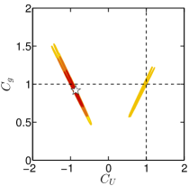
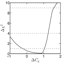
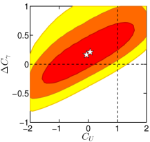
Figure 1 displays the results of this fit in the $\Delta C_{g}$ versus $\Delta C_{\gamma}$ plane. The best fit is obtained for $\Delta C_{\gamma}\simeq 0.43$, $\Delta C_{g}\simeq-0.09$, and has $\chi^{2}_{\rm min}=12.31$ for 19 degrees of freedom (d.o.f.), giving a $p$-value of $0.87$. The results of this fit are summarized in Table 4, together with the results of the other fits of this section.

Figure 1: Two parameter fit of $\Delta C_{\gamma}$ and $\Delta C_{g}$, assuming $C_{U}=C_{D}=C_{V}=1$ (Fit I). The red, orange and yellow ellipses show the 68%, 95% and 99.7% CL regions, respectively. The white star marks the best-fit point $\Delta C_{\gamma}=0.426$, $\Delta C_{g}=-0.086$.

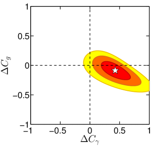
We note that the SM (i.e. $C_{U}=C_{D}=C_{V}=1$, $\Delta C_{g}=\Delta C_{\gamma}=0$) has $\chi^{2}=20.2$ and is hence more than $2\sigma$ away from the best fit in Fig. 1. The number of degrees of freedom for the SM fit is 21, implying a $p$-value of $0.51$. The largest $\chi^{2}$ contributions come from the $H\to\gamma\gamma$ channels from ATLAS ($\Delta\chi^{2}=5.06$), CMS ($\Delta\chi^{2}=3.36$) and Tevatron ($\Delta\chi^{2}=2.60$), followed by the VBF result for $H\to WW$ from CMS with $\Delta\chi^{2}=2.01$.

Fit II: varying $C_{U}$, $C_{D}$ and $C_{V}$ ($\Delta C_{\gamma}=\Delta C_{g}=0$)

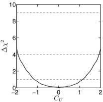
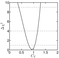
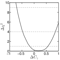
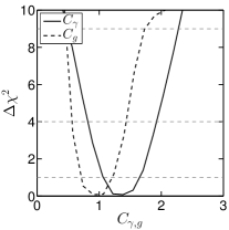
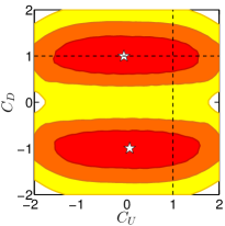
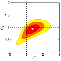
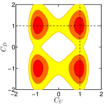
Next, we let $C_{U}$, $C_{D}$, $C_{V}$ vary, assuming there are no new particles contributing to the effective Higgs couplings to gluons and photons, i.e.  we take $\Delta C_{\gamma}=\Delta C_{g}=0$ implying $C_{g}=\overline{C}_{g}$, $C_{\gamma}=\overline{C}_{\gamma}$ as computed from the SM-particle loops. The results for the one-dimensional and two-dimensional $\chi^{2}$ distributions are shown in Figs. 2 and 3. The value of $C_{V}$ is rather well determined to be close to unity. It is intriguing that the best fit of $C_{V}$ is indeed just slightly below 1, as any model with only Higgs doublets or singlets requires $C_{V}\leq 1$. The best fit values for $C_{D}$ and $C_{U}$ are SM-like in that they have magnitudes that are close to one. However, the best fit $C_{U}$ value is opposite in sign to the SM Higgs case. The preference for $C_{U}<0$ is at the level of $2.6\sigma$ — see the first plot in Fig. 2. This results from the fact that an enhanced $\gamma\gamma$ rate (as observed in the experimental data) is obtained by changing the sign of the top-loop contribution so that it adds, rather than subtracts, from the $W$-loop. In contrast, in the case of $C_{D}$ almost equally good minima are found with $C_{D}<0$ and $C_{D}>0$. Details on the minima in different sectors of the ($C_{U}$, $C_{D}$) plane are given in Table 5. Note that, for the best fit point, the resulting $C_{\gamma}$ and $C_{g}$ are in good agreement with the result of Fit I above, for which $C_{\gamma}=1.43$ and $C_{g}=0.91$. Here, however, the enhanced $C_{\gamma}$ value derives from $C_{U}<0$ rather than from $\Delta C_{\gamma}\neq 0$. The best fit results are again tabulated in Table 4.

Figure 2: One-dimensional $\chi^{2}$ distributions for the three parameter fit, Fit II, of $C_{U}$, $C_{D}$, $C_{V}$ with $C_{\gamma}=\overline{C}_{\gamma}$ and $C_{g}=\overline{C}_{g}$ as computed in terms of $C_{U},C_{D},C_{V}$.

Figure 3: Two-dimensional $\chi^{2}$ distributions for the three parameter fit, Fit II, of $C_{U}$, $C_{D}$, $C_{V}$ with $C_{\gamma}=\overline{C}_{\gamma}$ and $C_{g}=\overline{C}_{g}$ as computed in terms of $C_{U},C_{D},C_{V}$. The red, orange and yellow ellipses show the 68%, 95% and 99.7% CL regions, respectively. The white star marks the best-fit point. Details on the minima in different sectors of the ($C_{U}$, $C_{D}$) plane can be found in Table 5.

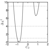
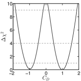
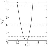
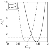
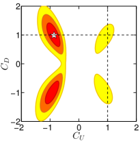
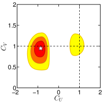
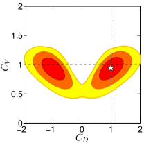
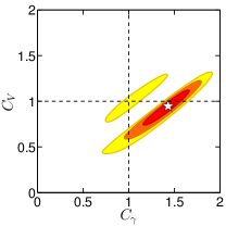
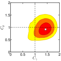
A negative sign of $C_{U}$—while maintaining a positive sign of $m_{t}$—is actually not easy to achieve. (A sign change of both $C_{U}$ and $m_{t}$ would have no impact on the top quark induced loop amplitudes.) It would require that $m_{t}$ is induced dominantly by the vev of a Higgs boson which is not the Higgs boson considered here. Hence, we have $C_{U}>0$ in most models, implying that it is important to study the impact of this constraint on our fits. The fit results when requiring $C_{U},C_{D}>0$ are shown in the left two plots of Fig. 4 and the top row of Fig. 5; see also Table 5. We observe that for this quadrant the results are consistent with SM expectations (i.e. within $\sim 1\sigma$). Interestingly the fit is not better than the SM itself: $\chi^{2}_{\rm min}=18.66$ for $21-3=18$ d.o.f., corresponding to $p=0.41$.

Figure 4: One-dimensional $\chi^{2}$ distributions for the three parameter fit, Fit II, but imposing $C_{U}>0$, $C_{D}>0$; the left two plots allow for $C_{V}>1$ ($\chi^{2}_{\rm min}=18.66$), while in the right two plots $C_{V}\leq 1$ ($\chi^{2}_{\rm min}=18.89$).

Figure 5: Two-dimensional $\chi^{2}$ distributions for the three parameter fit, Fit II, as in Fig. 3 but with $C_{U}>0$, $C_{D}>0$, $C_{V}>0$. The upper row of plots allows for $C_{V}>1$, while in the lower row of plots $C_{V}\leq 1$ is imposed.

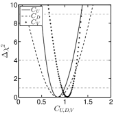
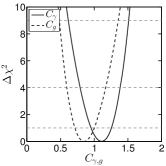
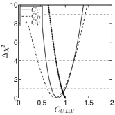
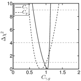
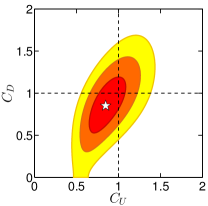
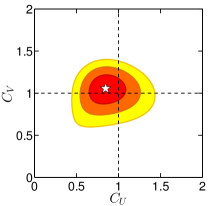
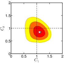
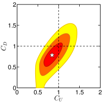
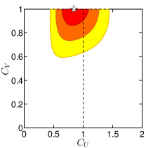
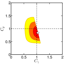
Another possible model constraint is to require $C_{V}\leq 1$ (recall that $C_{V}>0$ by convention). This constraint applies to any model containing only Higgs doublets and singlets. The 1d results for the combined requirement of $C_{U},C_{D}>0$ and $C_{V}\leq 1$ are shown in the right two plots of Fig. 4, and in the bottom-row plots of Fig. 5. We observe that the best fit values for $C_{U}$ and $C_{D}$ are only slightly shifted relative those found without constraining $C_{V}$, and that accordingly the $C_{\gamma}=\overline{C}_{\gamma}$ and $C_{g}=\overline{C}_{g}$ at the best fit point are only slightly shifted. However, the $C_{V}\leq 1$ constraint does severely change the upper bound on $C_{\gamma}$, which for $C_{U}>0$ and $\Delta C_{\gamma}=0$ mostly depends on the $W$-boson loop contribution. The apparent sharpness of the boundary in the $C_{g}$ vs. $C_{\gamma}$ plane is a result of the fact that these two quantities really only depend on $C_{U}$ for $C_{V}=1$.

Finally note that it has been shown in [69, 68] that single top production in association with a Higgs is greatly enhanced when $C_{U}$,$C_{V}$ have opposite signs. Thus, the possibility of $C_{U}<0$ should be further scrutinized by precision measurements of the single top production cross section at the LHC.

Fit	I	II	III, 1st min.	III, 2nd min.
$C_{U}$	$1$	$-0.86_{-0.16}^{+0.14}$	$-0.06\pm 1.30$	$\phantom{-}0.06\pm 1.30$
$C_{D}$	$1$	$\phantom{-}0.99_{-0.26}^{+0.28}$	$\phantom{-}1.00_{-0.26}^{+0.28}$	$-1.00_{-0.28}^{+0.26}$
$C_{V}$	$1$	$\phantom{-}0.95_{-0.13}^{+0.12}$	$\phantom{-}0.93_{-0.14}^{+0.12}$	$\phantom{-}0.93_{-0.14}^{+0.12}$
$\Delta C_{\gamma}$	$\phantom{-}0.43_{-0.16}^{+0.17}$	–	$\phantom{-}0.16_{-0.36}^{+0.38}$	$\phantom{-}0.21_{-0.39}^{+0.37}$
$\Delta C_{g}$	$-0.09\pm 0.10$	–	$\phantom{-}0.83_{-1.17}^{+0.24}$	$\phantom{-}0.83_{-1.17}^{+0.24}$
$C_{\gamma}$	$\phantom{-}1.43_{-0.16}^{+0.17}$	$\phantom{-}1.43\pm 0.17$	$\phantom{-}1.36_{-0.23}^{+0.26}$	$\phantom{-}1.36_{-0.23}^{+0.26}$
$C_{g}$	$\phantom{-}0.91\pm 0.10$	$\phantom{-}0.92_{-0.15}^{+0.17}$	$\phantom{-}0.95_{-0.23}^{+0.26}$	$\phantom{-}0.95_{-0.23}^{+0.26}$
$\chi^{2}_{\rm min}$	$12.31$	$11.95$	$11.46$	$11.46$
$\chi^{2}_{\rm min}/{\rm d.o.f.}$	$0.65$	$0.66$	$0.72$	$0.72$

Table 4: Summary of results for Fits I–III. For Fit II, the tabulated results are from the best fit, cf. column 1 of Table 5.

Sector	$C_{U}<0,\,C_{D}>0$	$C_{U},\,C_{D}<0$	$C_{U},\,C_{D}>0$
$C_{U}$	$-0.86_{-0.16}^{+0.14}$	$-0.91_{-0.17}^{+0.15}$	$0.85_{-0.13}^{+0.15}$
$C_{D}$	$\phantom{-}0.99_{-0.26}^{+0.28}$	$-0.98_{-0.27}^{+0.26}$	$0.85_{-0.21}^{+0.22}$
$C_{V}$	$\phantom{-}0.95_{-0.13}^{+0.12}$	$\phantom{-}0.94_{-0.13}^{+0.12}$	$1.06_{-0.12}^{+0.11}$
$C_{\gamma}$	$\phantom{-}1.43\pm 0.17$	$\phantom{-}1.43_{-0.17}^{+0.16}$	$1.11_{-0.16}^{+0.15}$
$C_{g}$	$\phantom{-}0.92_{-0.15}^{+0.17}$	$\phantom{-}0.91_{-0.15}^{+0.17}$	$0.85_{-0.13}^{+0.16}$
$\chi^{2}_{\rm min}$	11.95	12.06	18.66
$\chi^{2}_{\rm min}/{\rm d.o.f.}$	0.66	0.67	1.04

Table 5: Results for Fit II in different sectors of the ($C_{U}$, $C_{D}$) plane.

Fit III: varying $C_{U}$, $C_{D}$, $C_{V}$, $\Delta C_{\gamma}$ and $\Delta C_{g}$

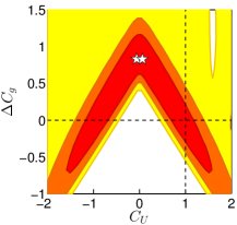
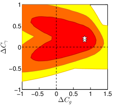
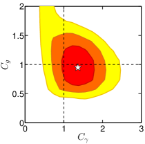
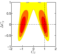
Finally, in Fit III, we allow the $\Delta C_{g}$ and $\Delta C_{\gamma}$ additions to $\overline{C}_{g}$ and $\overline{C}_{\gamma}$, fitting therefore to five free parameters: $C_{U}$, $C_{D}$, $C_{V}$, $\Delta C_{g}$, and $\Delta C_{\gamma}$. The associated 1d and 2d plots are given in Figs. 6 and 7. There are two main differences as compared to Fit II. On the one hand, the preference for $C_{\gamma}>1$ does does not necessarily imply a negative value for $C_{U}$, since a positive value for $\Delta C_{\gamma}$ can contribute to an increase in $C_{\gamma}$ even when the top-quark loop interferes destructively with the $W$ loop. (This is obviously already expected from Fit I.) On the other hand, both $C_{U}$ and $\Delta C_{g}$ feed into the effective $C_{g}$, and if one of them is large the other one has to be small to result in a near SM-like $gg\to H$ cross section. This anti-correlation between $|C_{U}|$ and $\Delta C_{g}$ can be seen in the center-top plot in Fig. 7. The best fit is actually obtained for $C_{U}\approx 0$, with $\Delta C_{g}\approx 1$ in order to compensate for the very suppressed top-loop contribution to ggF. However, it is also apparent that the minimum at $C_{U}=0$ is quite shallow (cf. the top left plot in Fig. 6) and that a fit with $C_{U}\approx 1$ with small $\Delta C_{g}$ is well within the $68\%$ contour (as should indeed be the case for consistency with Fits I and II).

We also note that at the best fit, i.e. that with $C_{U}\approx 0$, one finds $C_{\gamma}\sim\overline{C}_{\gamma}>1$ by virtue of the fact that the $W$ loop is not partially cancelled by the top loop and only a small $\Delta C_{\gamma}\sim 0.16$–$0.21$ is needed to further enhance the $\gamma\gamma$ final state and bring $\mu(\gamma\gamma)$ into agreement with observations; see top-right and bottom-right plots of Fig. 7. If we move to the SM value of $C_{U}=1$ then $\Delta C_{\gamma}\sim 0.45$ is needed to fit the $\gamma\gamma$ rate. The best fit results are tabulated in Table 4.

A way to lift the degeneracy in $C_{U}$ and $\Delta C_{g}$ would be to have an independent determination of $C_{U}$. This might be achieved by an accurate measurement of the ${\rm ttH}$ channel, as illustrated in Fig. 8. This figure assumes that $\mu({\rm ttH})$ will eventually be measured with 30% accuracy — more concretely, the figure assumes $\mu({\rm ttH})=1\pm 0.3$. This is certainly a very challenging task. For comparison, CMS currently gives $\mu({\rm ttH})\approx-0.8^{+2.2}_{-1.8}$ [12]. Finally, as mentioned above, $C_{U}$ may also be constrained by the associated production of a single top and a Higgs [69, 68].

Figure 6: One-dimensional $\chi^{2}$ distributions for the five parameter fit of $C_{U}$, $C_{D}$, $C_{V}$, $\Delta C_{\gamma}$ and $\Delta C_{g}$ (Fit III). Details regarding the best fit point are given in Table 4.

Figure 7: Two-dimensional distributions for the five parameter fit of $C_{U}$, $C_{D}$, $C_{V}$, $\Delta C_{\gamma}$ and $\Delta C_{g}$ (Fit III). Details regarding the best fit point are given in Table 4.

Figure 8: Lifting of the degeneracy in $C_{U}$ and $\Delta C_{g}$ in Fit III when $t\bar{t}H$ is measured to 30% accuracy ($\mu({\rm ttH})=1\pm 0.3$). These two plots should be compared to the top left and top middle plots of Fig. 7. See text for details.

3.2 Two-Higgs-Doublet Model

So far our fits have been model-independent, relying only on the Lagrangian structure of Eq. (2). Let us now turn to the concrete examples of Two-Higgs-Doublet Models (2HDMs) of Type I and Type II. In both cases, the basic parameters describing the coupling of either the light $h$ or heavy $H$ CP-even Higgs boson are only two: $\alpha$ (the CP-even Higgs mixing angle) and $\tan\beta=v_{u}/v_{d}$, where $v_{u}$ and $v_{d}$ are the vacuum expectation values of the Higgs field that couples to up-type quarks and down-type quarks, respectively. The Type I and Type II models are distinguished by the pattern of their fermionic couplings as given in Table 6. The SM limit for the $h$ ($H$) in the case of both Type I and Type II models corresponds to $\alpha=\beta-\pi/2$ ($\alpha=\beta$). In our discussion below, we implicitly assume that there are no contributions from non-SM particles to the loop diagrams for $C_{\gamma}$ and $C_{g}$. In particular, this means our results correspond to the case where the charged Higgs boson, whose loop might contribute to $C_{\gamma}$, is heavy.

	Type I and II	Type I		Type II
Higgs	VV	up quarks	down quarks &	up quarks	down quarks &
			leptons		leptons
$h$	$\sin(\beta-\alpha)$	$\cos\alpha/\sin\beta$	$\cos\alpha/\sin\beta$	$\cos\alpha/\sin\beta$	$-{\sin\alpha/\cos\beta}$
$H$	$\cos(\beta-\alpha)$	$\sin\alpha/\sin\beta$	$\sin\alpha/\sin\beta$	$\sin\alpha/\sin\beta$	$\cos\alpha/\cos\beta$
$A$	0	$\cot\beta$	$-\cot\beta$	$\cot\beta$	$\tan\beta$

Table 6: Tree-level vector boson couplings $C_{V}^{h_{i}}$ ($V=W,Z$) and fermionic couplings $C^{h_{i}}_{F}$ normalized to their SM values for the Type I and Type II two-Higgs-doublet models.

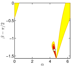
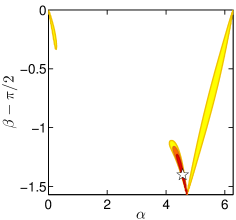
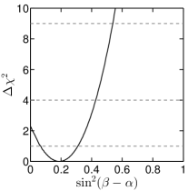
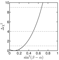
The results of the 2HDM fits are shown in Fig. 9 for the case that the state near 125 GeV is the lighter CP-even $h$. The figure also applies for the case of the heavier $H$ being identified with the $\sim 125~{}{\rm GeV}$ state with the replacement rules given in the figure caption. Note that the convention $C_{V}>0$ implies $\sin(\beta-\alpha)>0$ for the $h$ and $\cos(\beta-\alpha)>0$ for the $H$. Moreover, the requirement $\tan\beta>0$ restricts $\beta\in[0,\pi/2]$. The best fit values and $1\sigma$ ranges for $\alpha$ and $\beta$, together with the corresponding values for $C_{U}$, $C_{D}$, $C_{V}$, $C_{g}$ and $C_{g}$, are listed in Table 7. These numbers are again for the case of $h$ being the state near 125 GeV. Replacing $h$ by $H$ amounts to a shift in $\alpha\to\alpha+\pi/2$; thus we find $\alpha=6.07_{-0.08}^{+0.09}$ ($\cos\alpha=0.98\pm 0.02$) for the 2HDM-I and $\alpha=6.14_{-0.14}^{+0.15}$ ($\cos\alpha=0.99_{-0.03}^{+0.01}$) for the 2HDM-II, while the values for $\tan\beta$, $C_{U}$, $C_{D}$, $C_{V}$, etc. do not change.

Figure 9: 2HDM fits for the $h$ in the Type I (left) and Type II (right) models. The upper row shows the fit results in the $\beta-\pi/2$ vs. $\alpha$ plane, while the lower row shows the $\sin\beta$ vs. $\cos\alpha$ plane. The dashed lines indicate the SM limit. The same results are obtained for the heavier $H$ with the replacements $\beta-\pi/2\to\beta$ and $\alpha\to\alpha+\pi/2$ ($\sin\beta\to-\cos\beta$, $\cos\alpha\to\sin\alpha$).

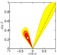
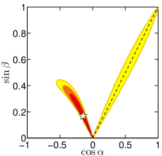
Fit	2HDM-I	2HDM-II	2HDM-I, $\tan\beta>1$	2HDM-II, $\tan\beta>1$
$\alpha$ [rad]	$\phantom{-}4.50_{-0.08}^{+0.09}$	$\phantom{-}4.56_{-0.14}^{+0.15}$	$5.37_{-0.13}^{+1.11}$	$6.28_{-0.83}^{+0.17}$
$\beta$ [rad]	$\phantom{-}0.24_{-0.10}^{+0.07}$	$\phantom{-}0.17_{-0.17}^{+0.12}$	$[\pi/4,\,\pi/2]$	$1.56_{-0.78}^{+0.01}$
$\cos\alpha$	$-0.21_{-0.08}^{+0.09}$	$-0.15_{-0.13}^{+0.15}$	$0.61_{-0.11}^{+0.39}$	$1.00_{-0.67}$
$\tan\beta$	$\phantom{-}0.24_{-0.10}^{+0.08}$	$\phantom{-}0.17_{-0.17}^{+0.13}$	$[1,\,+\infty[$	$[1,\,+\infty[$
$C_{U}$	$-0.90_{-0.19}^{+0.17}$	$-0.87_{-0.13}^{+0.12}$	$0.87_{-0.15}^{+0.17}$	$1.02_{-0.07}^{+0.05}$
$C_{D}$	$-0.90_{-0.19}^{+0.17}$	$\phantom{-}1.00_{-0.01}$	$0.87_{-0.15}^{+0.17}$	$0.94_{-0.11}^{+0.13}$
$C_{V}$	$\phantom{-}0.90\pm 0.07$	$\phantom{-}0.95_{-0.12}^{+0.05}$	$0.99_{-0.04}^{+0.01}$	$1.00_{-0.05}$
$C_{\gamma}$	$\phantom{-}1.37_{-0.10}^{+0.09}$	$\phantom{-}1.44_{-0.13}^{+0.08}$	$1.03_{-0.06}$	$1.01_{-0.09}^{+0.01}$
$C_{g}$	$\phantom{-}0.90_{-0.16}^{+0.19}$	$\phantom{-}0.92_{-0.11}^{+0.13}$	$0.87_{-0.15}^{+0.16}$	$0.99_{-0.04}^{+0.08}$
$\chi^{2}_{\rm min}$	12.20	11.95	19.43	19.88

Table 7: Summary of fit results for the $h$ in 2HDMs of Type I and Type II.

Note that for both the Type I and the Type II model, the best fits are quite far from the SM limit in parameter space. In particular, since we do not include any extra loop contributions to $C_{\gamma}$, we end up with negative $C_{U}$ close to $-1$ as in Fit II. Demanding $C_{U}>0$ (i.e. $\cos\alpha>0$ for $h$, $\sin\alpha>0$ for $H$), one ends up in a long ‘valley’ along the decoupling limit where the Higgs couplings are SM like, see Fig. 9; this is however always more than $2\sigma$ away from the best fit. Furthermore, solutions with very small $\tan\beta<1$ are preferred at more than $2\sigma$. Since such small values of $\tan\beta$ are rather problematic (in particular $\tan\beta<0.5$ is problematical for maintaining a perturbative magnitude for the top-quark Yukawa coupling) we also give in Table 7 the corresponding fit results requiring $\tan\beta>1$. These results come quite close to the SM limit, and accordingly have a $\chi^{2}_{\rm min}$ of about 19–20 (recall that for the SM we find $\chi^{2}\simeq 20.2$). 2HDMs with $\tan\beta>1$ hence do not provide a better fit than the SM itself.

A couple of more comments are in order. First, an important question that we leave for future work is whether other — e.g. stability, unitarity, perturbativity (SUP) and precision electroweak (PEW) — constraints are obeyed at the best-fit points, or the 68% CL regions. Here we just note that according to Fig. 1 of [70], the SUP and PEW constraints do not seem problematic for Type II, but may play a role for Type I models at low $\tan\beta$.

Second, the best fits correspond to very small $\tan\beta$ (small $\beta$) values that are potentially constrained by limits from B-physics, in particular from $\Delta M_{Bs}$ and $Z\to b\bar{b}$ . The B-physics constraints are summarized in Figs. 15 and 18 of [71] for Type II and Type I, respectively. Figure 18 for Type I places a lower bound on $\tan\beta$ as a function of the charged Higgs mass which excludes small $\tan\beta<1$ unless the charged Higgs is very heavy, something that is possible but somewhat unnatural. Figure 15 for Type II places a substantial lower bound on the charged Higgs mass for all $\tan\beta$, but such a constraint does not exclude the 68% CL region.

Third, we remind the reader that in the 2HDMs, the soft $Z_{2}$-symmetry-breaking $m_{12}^{2}$ and the other Higgs masses ($M_{h}$, $M_{H}$ and $M_{A}$) are independent parameters. It is thus possible to have either $M_{h}$ or $M_{H}\sim 125~{}{\rm GeV}$ without violating constraints from direct searches for the charged Higgs whose mass is related to $m_{A}$. However, in the case of $M_{H}\sim 125~{}{\rm GeV}$, one has to avoid the LEP limits for the lighter $h$, which severely constrain the $h$ coupling to $ZZ$ in case of $M_{h}<114~{}{\rm GeV}$ [72]. So either $M_{h}\gtrsim 114~{}{\rm GeV}$ for $M_{H}\approx 125~{}{\rm GeV}$, or $\sin^{2}(\beta-\alpha)$ needs to be small (e.g. $\sin^{2}(\beta-\alpha)\lesssim 0.3$ for $M_{h}\approx 100~{}{\rm GeV}$, or $\sin^{2}(\beta-\alpha)\lesssim 0.1$ for $M_{h}<90~{}{\rm GeV}$). The $\Delta\chi^{2}$ distributions of $\sin^{2}(\beta-\alpha)$ for Type I and Type II with $M_{H}\sim 125~{}{\rm GeV}$ are shown in Fig. 10. Interestingly, around the best fit the $h$ coupling to $ZZ$ is sufficiently suppressed to allow for $M_{h}$ of the order of $100~{}{\rm GeV}$ (or lower in Type II).

Figure 10: $\Delta\chi^{2}$ distribution of $\sin^{2}(\beta-\alpha)$ in the Type I (left) and Type II (right) models for the case that $H$ is the observed state near 125 GeV.

4 Summary and Conclusions

We assessed to which extend the currently available data on the Higgs-like scalar constrain the Higgs couplings. To this end we performed fits to all public data from the LHC and the Tevatron experiments.

First, we employed a general parametrization of the Higgs couplings based on a SM-like Lagrangian, but allowing for extra contributions to the loop-induced couplings of the Higgs-like scalar to gluons and photons. While the SM does not provide a bad fit ($\chi^{2}/{\rm d.o.f.}=0.96$), it is more than $2\sigma$ away from our best fit solutions. The main pull comes from the enhanced $H\to\gamma\gamma$ rates observed by ATLAS and CMS, as well as from the Tevatron experiments. The best fits are thus obtained when either $C_{U}\sim-1$ (i.e. opposite in sign to the SM expectation) or there is a large BSM contribution to the $\gamma\gamma$ coupling of the Higgs. In short, significant deviations from the SM values are preferred by the currently available data and should certainly be considered viable. Since having $C_{U}\sim-1$ (in the $C_{V}>0$ convention) is not easy to achieve in a realistic model context, and leads to unitarity violation in $WW\rightarrow t\bar{t}$ scattering at scales that can be as low as 5 TeV [73, 74], it would seem that new physics contributions to the effective couplings of the Higgs to gluons and photons are the preferred option. (The possibility of a second, degenerate Higgs boson contributing to the observed signal remains another interesting option, not considered here.)

Second, we examined how well 2HDM models of Type I and Type II fit the data. We found that it is possible to obtain a good fit in these models with $\sin(\beta-\alpha)$ ($\cos(\beta-\alpha)$), in the $h$ ($H$) cases, respectively, not far from $1$. However, the best fit values for the individual $C_{U}$, $C_{D}$, $C_{\gamma}$ and $C_{g}$ parameters lie far from their SM values. Further, the best fits give $\tan\beta<1$, which is disfavored from the theoretical point of view if we want perturbativity up to the GUT scale. Requiring $\tan\beta>1$ (or simply $C_{U}>0$) pushes the fit into the SM ‘valley’ and no improvement over the pure SM solution is obtained. In particular the $\chi^{2}$ obtained in this region is substantially larger than that for the best fit, and not far from the $\chi^{2}$ found for the SM.

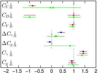
We once again refer the reader to Tables 4, 5 and 7 which summarize the best fit values and $1\sigma$ errors for the parameters for the various cases considered. In Fig. 11 we show some of these results graphically. Moreover, in order to assess the physics associated with our best fit points, we give in Tables 8 and 9 the values of the derived (theory level) signal strengths $\widehat{\mu}({\rm ggF},\gamma\gamma)$, $\widehat{\mu}({\rm ggF},ZZ)$, $\widehat{\mu}({\rm ggF},b\overline{b})$, $\widehat{\mu}({\rm VBF},\gamma\gamma)$, $\widehat{\mu}({\rm VBF},ZZ)$, and $\widehat{\mu}({\rm VBF},b\overline{b})$ for the best fit point in the various fits we have considered. (These are a complete set since for the models we consider $\widehat{\mu}(X,\tau\tau)=\widehat{\mu}(X,b\overline{b})$, $\widehat{\mu}(X,WW)=\widehat{\mu}(X,ZZ)$ and $\widehat{\mu}({\rm VBF},Y)=\widehat{\mu}({\rm VH},Y)$.) We see that in the general case both $\widehat{\mu}({\rm ggF},\gamma\gamma)$ and $\widehat{\mu}({\rm VBF},\gamma\gamma)$ are enhanced by factors 1.7–2.1 (1.8–1.9 in 2HDMs), while the other signal strengths tend to be $\lesssim 1$. When demanding $C_{U}>0$ without allowing for extra contributions from new particles, then only very small enhancements of $\widehat{\mu}({\rm VBF},\gamma\gamma)$ and $\widehat{\mu}({\rm VBF},ZZ)$ of the order of 1.2–1.3 are found.

Last but not least, we strongly encourage the experimental collaborations to make as complete as possible channel-by-channel information (including the important decomposition into production modes) available, in order to allow for reliable tests of non-standard Higgs scenarios. The information currently given by ATLAS and CMS for the $\gamma\gamma$ signal is an example of good practice and should become the standard for the presentation of results for all channels. This would immensely help interpretation efforts such as attempted in this paper. The ideal case would of course be if the full likelihood distributions were made available.

Figure 11: Graphical representation of the best fit values for $C_{U}$, $C_{D}$, $C_{V}$, $\Delta C_{\gamma}$ and $\Delta C_{g}$ of Table 4. The labels refer to the fits discussed in the text. The dashed lines indicate the SM value for the given quantity. The $\times$’s indicate cases where the parameter in question was fixed to its SM value.

Fit	I	II, $C_{U}<0$	II, $C_{U}>0$	III
$\widehat{\mu}({\rm ggF},\gamma\gamma)$	$1.71_{-0.32}^{+0.33}$	$1.81_{-0.41}^{+0.43}$	$1.07\pm 0.18$	$1.79_{-0.34}^{+0.36}$
$\widehat{\mu}({\rm ggF},ZZ)$	$0.84_{-0.17}^{+0.18}$	$0.79\pm 0.15$	$0.97\pm 0.20$	$0.84_{-0.18}^{+0.21}$
$\widehat{\mu}({\rm ggF},b\overline{b})$	$0.84_{-0.17}^{+0.18}$	$0.87_{-0.40}^{+0.57}$	$0.63_{-0.26}^{+0.36}$	$0.96_{-0.43}^{+0.59}$
$\widehat{\mu}({\rm VBF},\gamma\gamma)$	$2.05_{-0.44}^{+0.54}$	$1.92_{-0.68}^{+0.78}$	$1.66_{-0.63}^{+0.70}$	$1.74_{-0.73}^{+0.84}$
$\widehat{\mu}({\rm VBF},ZZ)$	$1.00\pm 0.02$	$0.84_{-0.36}^{+0.42}$	$1.50_{-0.46}^{+0.50}$	$0.82_{-0.35}^{+0.38}$
$\widehat{\mu}({\rm VBF},b\overline{b})$	$1.00\pm 0.02$	$0.92\pm 0.30$	$0.98\pm 0.32$	$0.93_{-0.29}^{+0.25}$

Table 8: Summary of $\widehat{\mu}$ results for Fits I–III. For Fit II, the tabulated results are for the best fit with $C_{U}<0$, column 1 of Table 5, and for the case $C_{U},C_{D}>0$, column 3 of Table 5.

Fit	2HDM-I	2HDM-II	2HDM-I, $\tan\beta>1$	2HDM-II, $\tan\beta>1$
$\widehat{\mu}({\rm ggF},\gamma\gamma)$	$1.86_{-0.38}^{+0.41}$	$1.81_{-0.40}^{+0.41}$	$0.97_{-0.09}^{+0.03}$	$1.08_{-0.26}^{+0.25}$
$\widehat{\mu}({\rm ggF},ZZ)$	$0.81\pm 0.11$	$0.79_{-0.18}^{+0.17}$	$0.91_{-0.13}^{+0.10}$	$1.08_{-0.21}^{+0.17}$
$\widehat{\mu}({\rm ggF},b\overline{b})$	$0.80_{-0.37}^{+0.54}$	$0.88_{-0.29}^{+0.35}$	$0.70_{-0.27}^{+0.37}$	$0.96_{-0.14}^{+0.24}$
$\widehat{\mu}({\rm VBF},\gamma\gamma)$	$1.87_{-0.65}^{+0.77}$	$1.91_{-0.63}^{+0.36}$	$1.27_{-0.34}^{+0.33}$	$1.08_{-0.26}^{+0.16}$
$\widehat{\mu}({\rm VBF},ZZ)$	$0.81_{-0.33}^{+0.41}$	$0.84_{-0.33}^{+0.20}$	$1.19_{-0.25}^{+0.21}$	$1.08_{-0.22}^{+0.16}$
$\widehat{\mu}({\rm VBF},b\overline{b})$	$0.81\pm 0.11$	$0.93_{-0.20}^{+0.10}$	$0.91_{-0.13}^{+0.10}$	$0.95_{-0.11}^{+0.10}$

Table 9: Summary of $\widehat{\mu}$ results for the interpretation in 2HDM models.

References

- [1] G. Aad et al. [ATLAS Collaboration], “Observation of a new particle in the search for the Standard Model Higgs boson with the ATLAS detector at the LHC,” Phys. Lett. B 716 (2012) 1 [arXiv:1207.7214 [hep-ex]].
- [2] S. Chatrchyan et al. [CMS Collaboration], “Observation of a new boson at a mass of 125 GeV with the CMS experiment at the LHC,” Phys. Lett. B 716 (2012) 30 [arXiv:1207.7235 [hep-ex]].
- [3] Tevatron New Physics Higgs Working Group and CDF and D0 Collaborations, “Updated Combination of CDF and D0 Searches for Standard Model Higgs Boson Production with up to 10.0 fb-1 of Data,” arXiv:1207.0449 [hep-ex].
- [4] ATLAS-CONF-2012-168, “Observation and study of the Higgs boson candidate in the two photon decay channel with the ATLAS detector at the LHC” (Dec 2012).
- [5] CMS-PAS-HIG-12-015, “Evidence for a new state decaying into two photons in the search for the standard model Higgs boson in pp collisions” (July 2012).
- [6] ATLAS-CONF-2012-169, “Updated results and measurements of properties of the new Higgs-like particle in the four lepton decay channel with the ATLAS detector” (Dec 2012).
- [7] CMS-PAS-HIG-12-041, “Updated results on the new boson discovered in the search for the standard model Higgs boson in the ZZ to 4 leptons channel in pp collisions at and 8 TeV” (Nov 2012).
- [8] ATLAS-CONF-2012-158, “Update of the Analysis with 13 fb or TeV Data Collected with the ATLAS Detector” (Nov 2012).
- [9] ATLAS-CONF-2012-162, “Updated ATLAS results on the signal strength of the Higgs-like boson for decays into WW and heavy fermion final states” (Nov 2012).
- [10] CMS-PAS-HIG-12-042, “Evidence for a particle decaying to in the fully leptonic final state in a standard model Higgs boson search in pp collisions at the LHC” (Nov 2012).
- [11] ATLAS-CONF-2012-170, “An update of combined measurements of the new Higgs-like boson with high mass resolution channels” (Dec 2012).
- [12] CMS-PAS-HIG-12-045, “Combination of standard model Higgs boson searches and measurements of the properties of the new boson with a mass near 125 GeV” (Nov 2012).
- [13] T. Aaltonen et al. [CDF and D0 Collaborations], “Evidence for a particle produced in association with weak bosons and decaying to a bottom-antibottom quark pair in Higgs boson searches at the Tevatron,” Phys. Rev. Lett. 109 (2012) 071804 [arXiv:1207.6436 [hep-ex]].
-
[14]
Yuji Enari, “ from Tevatron”, talk at HCP2012, 14 Nov 2012, Kyoto, Japan,
http://kds.kek.jp/conferenceDisplay.py?confId=10808. - [15] ATLAS-CONF-2012-127, “Coupling properties of the new Higgs-like boson observed with the ATLAS detector at the LHC” (Sep 2012).
- [16] D. Carmi, A. Falkowski, E. Kuflik and T. Volansky, “Interpreting LHC Higgs Results from Natural New Physics Perspective,” JHEP 1207 (2012) 136 [arXiv:1202.3144 [hep-ph]].
- [17] A. Azatov, R. Contino and J. Galloway, “Model-Independent Bounds on a Light Higgs,” JHEP 1204 (2012) 127 [arXiv:1202.3415 [hep-ph]].
- [18] J. R. Espinosa, C. Grojean, M. Muhlleitner and M. Trott, “Fingerprinting Higgs Suspects at the LHC,” JHEP 1205 (2012) 097 [arXiv:1202.3697 [hep-ph]].
- [19] M. Klute, R. Lafaye, T. Plehn, M. Rauch and D. Zerwas, “Measuring Higgs Couplings from LHC Data,” Phys. Rev. Lett. 109 (2012) 101801 [arXiv:1205.2699 [hep-ph]].
- [20] A. Azatov, S. Chang, N. Craig and J. Galloway, “Higgs fits preference for suppressed down-type couplings: Implications for supersymmetry,” Phys. Rev. D 86 (2012) 075033 [arXiv:1206.1058 [hep-ph]].
- [21] D. Carmi, A. Falkowski, E. Kuflik and T. Volansky, “Interpreting the Higgs,” arXiv:1206.4201 [hep-ph].
- [22] I. Low, J. Lykken and G. Shaughnessy, “Have We Observed the Higgs (Imposter)?,” arXiv:1207.1093 [hep-ph].
- [23] T. Corbett, O. J. P. Eboli, J. Gonzalez-Fraile and M. C. Gonzalez-Garcia, “Constraining anomalous Higgs interactions,” Phys. Rev. D 86 (2012) 075013 [arXiv:1207.1344 [hep-ph]].
- [24] P. P. Giardino, K. Kannike, M. Raidal and A. Strumia, “Is the resonance at 125 GeV the Higgs boson?,” arXiv:1207.1347 [hep-ph].
- [25] J. Ellis and T. You, “Global Analysis of the Higgs Candidate with Mass 125 GeV,” JHEP 1209 (2012) 123 [arXiv:1207.1693 [hep-ph]].
- [26] M. Montull and F. Riva, “Higgs discovery: the beginning or the end of natural EWSB?,” JHEP 1211 (2012) 018 [arXiv:1207.1716 [hep-ph]].
- [27] J. R. Espinosa, C. Grojean, M. Muhlleitner and M. Trott, “First Glimpses at Higgs’ face,” arXiv:1207.1717 [hep-ph].
- [28] D. Carmi, A. Falkowski, E. Kuflik, T. Volansky and J. Zupan, “Higgs After the Discovery: A Status Report,” JHEP 1210 (2012) 196 [arXiv:1207.1718 [hep-ph]].
- [29] S. Banerjee, S. Mukhopadhyay and B. Mukhopadhyaya, “New Higgs interactions and recent data from the LHC and the Tevatron,” JHEP 1210 (2012) 062 [arXiv:1207.3588 [hep-ph]].
- [30] F. Bonnet, T. Ota, M. Rauch and W. Winter, “Interpretation of precision tests in the Higgs sector in terms of physics beyond the Standard Model,” arXiv:1207.4599 [hep-ph].
- [31] T. Plehn and M. Rauch, “Higgs Couplings after the Discovery,” Europhys. Lett. 100 (2012) 11002 [arXiv:1207.6108 [hep-ph]].
- [32] J. R. Espinosa, C. Grojean, V. Sanz and M. Trott, “NSUSY fits,” arXiv:1207.7355 [hep-ph].
- [33] D. Elander and M. Piai, “The decay constant of the holographic techni-dilaton and the 125 GeV boson,” arXiv:1208.0546 [hep-ph].
- [34] A. Djouadi, “Precision Higgs coupling measurements at the LHC through ratios of production cross sections,” arXiv:1208.3436 [hep-ph].
- [35] W. Altmannshofer, S. Gori and G. D. Kribs, “A Minimal Flavor Violating 2HDM at the LHC,” arXiv:1210.2465 [hep-ph].
- [36] B. A. Dobrescu and J. D. Lykken, “Coupling spans of the Higgs-like boson,” arXiv:1210.3342 [hep-ph].
- [37] S. Chang, S. K. Kang, J. -P. Lee, K. Y. Lee, S. C. Park and J. Song, “Comprehensive study of two Higgs doublet model in light of the new boson with mass around 125 GeV,” arXiv:1210.3439 [hep-ph].
- [38] G. Moreau, “Constraining extra-fermion(s) from the Higgs boson data,” arXiv:1210.3977 [hep-ph].
- [39] G. Cacciapaglia, A. Deandrea, G. D. La Rochelle and J. -B. Flament, “Higgs couplings beyond the Standard Model,” arXiv:1210.8120 [hep-ph].
- [40] P. Bechtle, S. Heinemeyer, O. Stal, T. Stefaniak, G. Weiglein and L. Zeune, “MSSM Interpretations of the LHC Discovery: Light or Heavy Higgs?,” arXiv:1211.1955 [hep-ph].
- [41] T. Corbett, O. J. P. Eboli, J. Gonzalez-Fraile and M. C. Gonzalez-Garcia, “Robust Determination of the Higgs Couplings: Power to the Data,” arXiv:1211.4580 [hep-ph].
- [42] E. Masso and V. Sanz, “Limits on Anomalous Couplings of the Higgs to Electroweak Gauge Bosons from LEP and LHC,” arXiv:1211.1320 [hep-ph].
- [43] A. Azatov and J. Galloway, “Electroweak Symmetry Breaking and the Higgs Boson: Confronting Theories at Colliders,” arXiv:1212.1380 [hep-ph].
- [44] Hadron Collider Physics Symposium 2012 (HCP 2012), 12–16 Nov 2012, Kyoto, Japan, http://www.icepp.s.u-tokyo.ac.jp/hcp2012/
[45]
Status of the LHC and Experiments, CERN seminars, 13 Dec 2012,
http://indico.cern.ch/conferenceDisplay.py?confId=219381 - [46] J. R. Espinosa, M. Muhlleitner, C. Grojean and M. Trott, “Probing for Invisible Higgs Decays with Global Fits,” JHEP 1209 (2012) 126 [arXiv:1205.6790 [hep-ph]].
- [47] J. F. Gunion, Y. Jiang and S. Kraml, “Could two NMSSM Higgs bosons be present near 125 GeV?,” Phys. Rev. D 86 (2012) 071702 [arXiv:1207.1545 [hep-ph]].
- [48] P. M. Ferreira, H. E. Haber, R. Santos and J. P. Silva, “Mass-degenerate Higgs bosons at 125 GeV in the Two-Higgs-Doublet Model,” arXiv:1211.3131 [hep-ph].
- [49] J. F. Gunion, Y. Jiang and S. Kraml, “Diagnosing Degenerate Higgs Bosons at 125 GeV,” arXiv:1208.1817 [hep-ph].
- [50] ATLAS-CONF-2012-161, “Search for the Standard Model Higgs boson in produced in association with a vector boson and decaying to bottom quarks with the ATLAS detector” (Nov 2012).
- [51] ATLAS-CONF-2012-160, “Search for the Standard Model Higgs boson in decays in proton-proton collisions with the ATLAS detector” (Nov 2012).
- [52] CMS-PAS-HIG-12-039, “Search for SM Higgs in ” (Nov 2012).
- [53] CMS-PAS-HIG-12-025, “Search for Higgs boson production in association with top quark pairs in pp collisions” (July 2012).
- [54] CMS-PAS-HIG-12-044, “Search for the standard model Higgs boson produced in association with W or Z bosons, and decaying to bottom quarks for HCP 2012” (Nov 2012).
- [55] CMS-PAS-HIG-12-051, “Search for the standard model Higgs boson decaying to tau pairs produced in association with a W or Z boson” (Nov 2012).
- [56] CMS-PAS-HIG-12-043, “Search for the standard model Higgs boson decaying to tau pairs” (Nov 2012).
- [57] https://twiki.cern.ch/twiki/bin/view/LHCPhysics/CrossSections
- [58] A. de Roeck, private communication.
[59]
Aurelio Juste, “Standard Modek Higgs boson searches at the Tevatron ”, talk at HCP2012, 15 Nov 2012, Kyoto, Japan,
http://kds.kek.jp/conferenceDisplay.py?confId=9237. - [60] LHC Higgs Cross Section Working Group, A. David, A. Denner, M. Duehrssen, M. Grazzini, C. Grojean, G. Passarino and M. Schumacher et al., “LHC HXSWG interim recommendations to explore the coupling structure of a Higgs-like particle,” arXiv:1209.0040 [hep-ph].
- [61] M. Spira, “HIGLU: A program for the calculation of the total Higgs production cross-section at hadron colliders via gluon fusion including QCD corrections,” hep-ph/9510347.
- [62] M. Spira, “HIGLU and HDECAY: Programs for Higgs boson production at the LHC and Higgs boson decay widths,” Nucl. Instrum. Meth. A 389, 357 (1997) [hep-ph/9610350].
- [63] A. Djouadi, J. Kalinowski and M. Spira, “HDECAY: A Program for Higgs boson decays in the standard model and its supersymmetric extension,” Comput. Phys. Commun. 108, 56 (1998) [hep-ph/9704448].
- [64] F. James and M. Roos, “Minuit: A System for Function Minimization and Analysis of the Parameter Errors and Correlations,” Comput. Phys. Commun. 10 (1975) 343.
- [65] S. Kraml, et al., “Searches for New Physics: Les Houches Recommendations for the Presentation of LHC Results,” Eur. Phys. J. C 72 (2012) 1976 [arXiv:1203.2489 [hep-ph]].
- [66] F. J. Petriello, “Kaluza-Klein effects on Higgs physics in universal extra dimensions,” JHEP 0205 (2002) 003 [hep-ph/0204067].
- [67] G. Bélanger, A. Belyaev, M. Brown, M. Kakizaki and A. Pukhov, “Testing Minimal Universal Extra Dimensions Using Higgs Boson Searches at the LHC,” arXiv:1207.0798 [hep-ph].
- [68] M. Farina, C. Grojean, F. Maltoni, E. Salvioni and A. Thamm, “Lifting degeneracies in Higgs couplings using single top production in association with a Higgs boson,” arXiv:1211.3736 [hep-ph].
- [69] S. Biswas, E. Gabrielli and B. Mele, “Single top and Higgs associated production as a probe of the coupling sign at the LHC,” arXiv:1211.0499 [hep-ph].
- [70] A. Drozd, B. Grzadkowski, J. F. Gunion and Y. Jiang, “Two-Higgs-Doublet Models and Enhanced Rates for a 125 GeV Higgs,” arXiv:1211.3580 [hep-ph].
- [71] G. C. Branco, P. M. Ferreira, L. Lavoura, M. N. Rebelo, M. Sher and J. P. Silva, “Theory and phenomenology of two-Higgs-doublet models,” Phys. Rept. 516, 1 (2012) [arXiv:1106.0034 [hep-ph]].
- [72] P. Teixeira-Dias, “Higgs boson searches at LEP,” J. Phys. Conf. Ser. 110 (2008) 042030 [arXiv:0804.4146 [hep-ex]].
- [73] D. Choudhury, R. Islam, A. Kundu and B. Mukhopadhyaya, “Anomalous Higgs Couplings as a Window to New Physics,” arXiv:1212.4652 [hep-ph].
- [74] G. Bhattacharyya, D. Das and P. B. Pal, “Modified Higgs couplings and unitarity violation,” arXiv:1212.4651 [hep-ph].