Merging H/W/Z + 0 and 1 jet at NLO with no merging scale: a path to parton shower + NNLO matching

Keith Hamilton
Theory Division, CERN, CH–1211, Geneva 23, Switzerland
E-mail
On leave from University College London. keith.hamilton@cern.ch
   Paolo Nason
INFN, Sezione di Milano Bicocca, Piazza della Scienza 3, 20126 Milan, Italy
E-mail
paolo.nason@mib.infn.it
   Carlo Oleari
Università di Milano-Bicocca and INFN, Sezione di Milano-Bicocca
Piazza della Scienza 3, 20126 Milan, Italy
E-mail
Carlo.Oleari@mib.infn.it
   Giulia Zanderighi
Rudolf Peierls Centre for Theoretical Physics, 1 Keble Road, University of Oxford, UK
E-mail
g.zanderighi1@physics.ox.ac.uk
Abstract:

We consider the POWHEG generator for a H/W/Z boson plus one jet, augmented with the recently proposed MiNLO method for the choice of scales and the inclusion of Sudakov form factors. Within this framework, the generator covers all the transverse-momentum region of the H/W/Z boson, i.e. no generation cuts are needed to obtain a finite result. By construction, the generator achieves NLO accuracy for distributions involving a finite (and relatively large) transverse momentum of the boson. We examine the conditions under which also the totally inclusive distributions (e.g. the boson rapidity distribution) achieve NLO accuracy. We find that a minimal modification of the MiNLO prescription is sufficient to achieve such accuracy. We thus construct a NLO generator for H/W/Z boson plus one jet production such that it smoothly merges into a NLO single boson production in the small transverse-momentum region. We notice that, by simply reweighting the boson rapidity distribution to NNLO predictions, we achieve a NNLO accurate generator matched to a shower. The approach applies to all production processes involving a colorless massive system plus one jet. We discuss how it may be extended to general processes.

QCD, Phenomenological Models, Hadronic Colliders
preprint: CERN-PH-TH/2012-356
LPN12-140, MCnet-12-15
OUTP-13-04P

1 Introduction

In recent times, next-to-leading order parton shower (NLO+PS) matching techniques have been developed and realised as practical simulation tools  [1, 2, 3]. The programs and methods underlying them have matured to the point where they are routinely used in LHC data analysis.

NLO+PS methods can also be applied to processes involving associated jet production at leading order. In the case of Higgs boson production, for example, there exist POWHEG simulations for inclusive production of a Higgs boson (the H generator from now on) [4], Higgs boson production with an associated jet (HJ), and also for the case of two associated jets (HJJ[5]. These simulations overlap in their population of phase space. However, the relative accuracies of each one in the various regions is complementary. Specifically, the H generator yields NLO accurate inclusive Higgs boson distributions, describing the radiation of a single jet with leading-order (LO) accuracy and the radiation of more than one jet with the accuracy of the shower to which it is interfaced (the collinear, leading-log, approximation). On the other hand, the HJ generator gives NLO precision for observables inclusive in the production of a Higgs boson plus one jet; it has only LO quality if we require two jets, with further radiation generated in the parton shower approximation. The HJ generator cannot be used to describe inclusive jet cross sections, since the NLO calculation on which it is based requires the presence of at least one jet. Similar considerations hold for the HJJ generator.

It is natural to ask whether one can merge the H, HJ and HJJ simulations, in such a way that all classes of observables have NLO accuracy in the end results. That is to say, one would ideally like to have a unified NLO+PS simulation, or simulation output, yielding inclusive Higgs boson distributions accurate at the NLO level, αS3superscriptsubscript𝛼S3\alpha_{\mathchoice{\displaystyle}{\scriptstyle}{\scriptscriptstyle}{\scriptscriptstyle}\rm S}^{3}, and, at the same time, distributions involving the Higgs boson plus one jet accurate at order αS4superscriptsubscript𝛼S4\alpha_{\mathchoice{\displaystyle}{\scriptstyle}{\scriptscriptstyle}{\scriptscriptstyle}\rm S}^{4}.

Several collaborations have addressed this merging problem [6, 7, 8, 9, 10, 11, 12, 13]. They all typically separate the output of each component simulation (the equivalent of H, HJ or HJJ) according to the jet multiplicity of the events it produces, discarding those having a multiplicity for which the generator does not possess the relevant NLO corrections. Having processed the output of each simulation in this way, the event samples are joined to give an inclusive sample. In a nutshell, each generator can therefore be regarded as contributing a single exclusive jet bin to the final inclusive sample, the magnitude of each bin being predominantly determined by the jet resolution scale used in performing the merging, the so-called merging scale. The merging scale is an unphysical parameter, and the dependence on it is, rightly, well studied in the implementations of the merging algorithms cited above, with different approaches invoking different means to mitigate the dependence on it. Relatedly, we point out that in all of the practical applications of NLO merging to date, the jet algorithms employed do not correspond to those currently used in LHC experimental analyses, albeit for good theoretical reasons: in particular, to lessen the dependence on the merging scale through the resummation of spurious large logarithmic corrections associated with it.

In all cases the choice of the merging scale poses a dilemma: if the merging scale is too low, the sample is dominated by the higher-multiplicity generators, while if it is chosen too large, one loses their benefit, since one is forced to describe relatively hard jets only with tree-level accuracy, or, worse still, with the parton-shower approximation.

To further clarify the situation consider again Higgs boson production. As stated above, the H generator yields 𝒪(αS3)𝒪superscriptsubscript𝛼S3{\cal O}(\alpha_{\mathchoice{\displaystyle}{\scriptstyle}{\scriptscriptstyle}{\scriptscriptstyle}\rm S}^{3}) accuracy for inclusive quantities, i.e. quantities that are integrated over the transverse momentum of the Higgs boson. Consider, however, the same integrated cross section up to a certain transverse momentum cut pTcutsuperscriptsubscript𝑝Tcutp_{\mathchoice{\displaystyle}{\scriptstyle}{\scriptscriptstyle}{\scriptscriptstyle}\rm T}^{\mathchoice{\displaystyle}{\scriptstyle}{\scriptscriptstyle}{\scriptscriptstyle}\rm cut}. Assuming that the Sudakov form factor provided by the NLO+PS implementation is next-to-leading log (NLL) accurate, missing next-to-next-to-leading log (NNLL) corrections to this quantity (corresponding to a factor exp[αS2L]1+αS2L+similar-toabsentsuperscriptsubscript𝛼S2𝐿similar-to1superscriptsubscript𝛼S2𝐿\sim\exp[\alpha_{\mathchoice{\displaystyle}{\scriptstyle}{\scriptscriptstyle}{\scriptscriptstyle}\rm S}^{2}L]\sim 1+\alpha_{\mathchoice{\displaystyle}{\scriptstyle}{\scriptscriptstyle}{\scriptscriptstyle}\rm S}^{2}L+..., where L=log(MH/pTcut)𝐿subscript𝑀𝐻superscriptsubscript𝑝TcutL=\log(M_{\scriptscriptstyle H}/p_{\mathchoice{\displaystyle}{\scriptstyle}{\scriptscriptstyle}{\scriptscriptstyle}\rm T}^{\mathchoice{\displaystyle}{\scriptstyle}{\scriptscriptstyle}{\scriptscriptstyle}\rm cut}), and MHsubscript𝑀𝐻M_{\scriptscriptstyle H} is the Higgs boson mass) reduce the accuracy of the distribution, depending upon the size of αSLsubscript𝛼S𝐿\alpha_{\mathchoice{\displaystyle}{\scriptstyle}{\scriptscriptstyle}{\scriptscriptstyle}\rm S}L. If we assume αSL21similar-tosubscript𝛼Ssuperscript𝐿21\alpha_{\mathchoice{\displaystyle}{\scriptstyle}{\scriptscriptstyle}{\scriptscriptstyle}\rm S}L^{2}\sim 1, as in the vicinity of the Sudakov region, these neglected NNLL terms are of relative order αS1.5superscriptsubscript𝛼S1.5\alpha_{\mathchoice{\displaystyle}{\scriptstyle}{\scriptscriptstyle}{\scriptscriptstyle}\rm S}^{1.5} with respect to the Born term. Thus, the NLO quality (that requires neglected terms to be of relative order αS2superscriptsubscript𝛼S2\alpha_{\mathchoice{\displaystyle}{\scriptstyle}{\scriptscriptstyle}{\scriptscriptstyle}\rm S}^{2} or higher) is lost. Thus, although the inclusive distributions are NLO accurate, the cut cross section may well not be if the cut is too low. Of course, if the cut is high enough the NLO precision is restored, since NLO+PS simulations describe the high transverse-momentum tail with tree-level accuracy and the fully integrated spectrum at the NLO level.

Turning now to look at the 𝙷𝙹𝙷𝙹{\tt HJ}{} generator from the same perspective, if we consider the cross section with a transverse momentum cut pT>pTcutsubscript𝑝Tsuperscriptsubscript𝑝Tcutp_{\mathchoice{\displaystyle}{\scriptstyle}{\scriptscriptstyle}{\scriptscriptstyle}\rm T}>p_{\mathchoice{\displaystyle}{\scriptstyle}{\scriptscriptstyle}{\scriptscriptstyle}\rm T}^{\mathchoice{\displaystyle}{\scriptstyle}{\scriptscriptstyle}{\scriptscriptstyle}\rm cut}, we know that large logarithmic corrections of the form αSL2subscript𝛼Ssuperscript𝐿2\alpha_{\mathchoice{\displaystyle}{\scriptstyle}{\scriptscriptstyle}{\scriptscriptstyle}\rm S}L^{2} relative to the Born term arise in the cross section, hence, if αSL21similar-tosubscript𝛼Ssuperscript𝐿21\alpha_{\mathchoice{\displaystyle}{\scriptstyle}{\scriptscriptstyle}{\scriptscriptstyle}\rm S}L^{2}\sim 1, the predictions completely fail. Some of the new NLO merging techniques attempt to resum these logarithmic corrections to all orders, in general though this resummation is, with the notable exception of ref. [11], limited to NLL contributions and with the neglect of the NNLL terms, as in the H case, leading to errors at the level of αS1.5similar-toabsentsuperscriptsubscript𝛼S1.5\sim\alpha_{\mathchoice{\displaystyle}{\scriptstyle}{\scriptscriptstyle}{\scriptscriptstyle}\rm S}^{1.5} terms relative to the leading-order cross section.

In order to avoid this problem, the authors of ref. [10], conservatively, use merging scales which are not too low. The authors of ref. [13] proposes to tackle the problem by forcing unitarity on the approach, using suitable subtractions in order to restore NLO accuracy. In ref. [11] the accuracy of the resummation is improved in order to reach the required precision for matching.

In the present work we study the possibility of building a NLO generator that does not lose NLO accuracy when the radiated parton is integrated over. In other words, we want to achieve the goals of merging without actually doing any merging at all.

In a recent paper [14], some of us have proposed a prescription (MiNLO: Multi-scale Improved NLO) for the choice of renormalization and factorization scales and the inclusion of Sudakov form factors in NLO calculations, such that the higher-multiplicity calculations seem to merge well with the lower-multiplicity ones. The numerical results of ref. [14] are quite striking, in that they seem to suggest that with this method, for example, the HJJ simulation yields a good description also for observables that are best computed with the HJ or H programs. In ref. [14], however, no arguments are given to justify this behaviour, and no attempt is made to quantify the formal accuracy that a generator which is NLO accurate in the description of (n+1)𝑛1(n+1)-jet observables has for those sensitive to m𝑚m jet topologies, with mn𝑚𝑛m\leq n.

In the present work, we address precisely these issues. We consider BJ generators, where B denotes either the Higgs (H), the W𝑊W (W) or the Z𝑍Z boson (Z) and ask the following questions:

  • How precise is the BJ generator, when improved with the MiNLO prescription, in describing inclusive boson production observables?

  • Is it possible to modify the MiNLO procedure in such a way that we achieve NLO accuracy also for these observables?

We will show that:

  • The inclusive boson observables are described by the BJ+MiNLO programs at relative order αSsubscript𝛼S\alpha_{\mathchoice{\displaystyle}{\scriptstyle}{\scriptscriptstyle}{\scriptscriptstyle}\rm S} with respect to the Born cross section. However, they do not reach NLO accuracy, since they also include ambiguous contributions of relative order αS1.5superscriptsubscript𝛼S1.5\alpha_{\mathchoice{\displaystyle}{\scriptstyle}{\scriptscriptstyle}{\scriptscriptstyle}\rm S}^{1.5}, rather than αS2superscriptsubscript𝛼S2\alpha_{\mathchoice{\displaystyle}{\scriptstyle}{\scriptscriptstyle}{\scriptscriptstyle}\rm S}^{2}.

  • The second question has a positive answer. In the main body of the paper we will clarify what needs to be done in order to gain genuine NLO precision for inclusive observables. The modifications needed for reaching this goal are simple and we have implemented them in our current MiNLO-POWHEG BOX HJ, WJ and ZJ generators.

  • As a final point, we notice that by reweighting the new BJ-MiNLO generators in such a way that the inclusive boson rapidity and decay kinematics are matched to the next-to-next-to-leading order (NNLO) result, one obtains a NNLO calculation matched to a parton shower simulation, i.e. a NNLO+PS generator.

The event generators built in this way can be further enhanced, so as to yield an improved description also for the third hardest emission, as proposed in ref. [7]. To this end, it is enough to simply feed the events obtained with the BJ-MiNLO programs through the relevant BJJ simulation, with the latter attaching the third hardest parton to the events with LL+LO accuracy.

The paper is organized as follows. In Section 2 we discuss the precision of the original BJ+MiNLO generator and the modifications that are necessary to attain NLO accuracy in the description of inclusive boson distributions. In Section 3 we give an alternative, more detailed proof. In Section 4 we present results obtained with our revised MiNLO approach and discuss issues related to the scale variation as an estimator of the theoretical error on the predictions. In Section 5 we show how we can improve the generators that we have constructed in order to achieve NNLO accuracy. In Section 6 we discuss briefly how the present findings may be generalized to more complex processes. Finally we present our conclusions in Section 7.

2 Accuracy of the BJ+MiNLO generators

2.1 Preliminaries

We want to determine the accuracy of the BJ+MiNLO generators when integrated over the boson transverse momentum at fixed rapidity. We will illustrate explicitly the case of Higgs boson plus jet production, but our findings hold trivially for WJ and ZJ as well, and for the production of a heavy colour-neutral system accompanied by one jet.

In order to avoid confusion, we will refer to the accuracy of inclusive results, integrated over the boson transverse momentum, as the (0)0\left(0\right) accuracy, and will refer instead to the accuracy in the H+j𝐻𝑗H+j inclusive cross section as the (1)1\left(1\right) accuracy. Thus, for example, by LO(0) and NLO(0) we mean leading (i.e. αS2superscriptsubscript𝛼S2\alpha_{\mathchoice{\displaystyle}{\scriptstyle}{\scriptscriptstyle}{\scriptscriptstyle}\rm S}^{2}) and next-to-leading (i.e. αS3superscriptsubscript𝛼S3\alpha_{\mathchoice{\displaystyle}{\scriptstyle}{\scriptscriptstyle}{\scriptscriptstyle}\rm S}^{3}) order accuracy in the Higgs boson inclusive rapidity distribution, and with LO(1) and NLO(1) we mean leading (i.e. αS3superscriptsubscript𝛼S3\alpha_{\mathchoice{\displaystyle}{\scriptstyle}{\scriptscriptstyle}{\scriptscriptstyle}\rm S}^{3}) and next-to-leading (i.e. αS4superscriptsubscript𝛼S4\alpha_{\mathchoice{\displaystyle}{\scriptstyle}{\scriptscriptstyle}{\scriptscriptstyle}\rm S}^{4}) order accuracy in the Higgs boson plus one jet distributions.

We focus upon the HJ generator with the MiNLO prescription. As illustrated in [14], this is obtained by modifying the POWHEG B¯¯𝐵\bar{B} function with the inclusion of the Sudakov form factor and with the use of appropriate scales for the couplings, according to the formula

B¯=αS2(MH2)αS(qT2)Δg2(MH,qT)[B(12Δg(1)(MH,qT))+V+𝑑ΦradR],¯𝐵superscriptsubscript𝛼S2superscriptsubscript𝑀𝐻2subscript𝛼Ssuperscriptsubscript𝑞T2superscriptsubscriptΔ𝑔2subscript𝑀𝐻subscript𝑞Tdelimited-[]𝐵12superscriptsubscriptΔ𝑔1subscript𝑀𝐻subscript𝑞T𝑉differential-dsubscriptΦrad𝑅\bar{B}=\alpha_{\mathchoice{\displaystyle}{\scriptstyle}{\scriptscriptstyle}{\scriptscriptstyle}\rm S}^{2}\left(M_{\scriptscriptstyle H}^{2}\right)\alpha_{\mathchoice{\displaystyle}{\scriptstyle}{\scriptscriptstyle}{\scriptscriptstyle}\rm S}\left(q_{\mathchoice{\displaystyle}{\scriptstyle}{\scriptscriptstyle}{\scriptscriptstyle}\rm T}^{2}\right)\Delta_{g}^{2}\left(M_{\scriptscriptstyle H},q_{\mathchoice{\displaystyle}{\scriptstyle}{\scriptscriptstyle}{\scriptscriptstyle}\rm T}\right)\left[B\left(1-2\Delta_{g}^{\left(1\right)}\left(M_{\scriptscriptstyle H},q_{\mathchoice{\displaystyle}{\scriptstyle}{\scriptscriptstyle}{\scriptscriptstyle}\rm T}\right)\right)+V+\int d\Phi_{{\rm rad}}\,R\right]\,, (1)

where we have stripped away three powers of αSsubscript𝛼S\alpha_{\mathchoice{\displaystyle}{\scriptstyle}{\scriptscriptstyle}{\scriptscriptstyle}\rm S} from the Born (B𝐵B), the virtual (V𝑉V) and the real (R𝑅R) contribution, factorizing them in front of eq. (1). We will comment later on the scale at which the remaining power of αSsubscript𝛼S\alpha_{\mathchoice{\displaystyle}{\scriptstyle}{\scriptscriptstyle}{\scriptscriptstyle}\rm S} in R𝑅R, V𝑉V and Δg(1)superscriptsubscriptΔ𝑔1\Delta_{g}^{\left(1\right)} is evaluated.

ΔgsubscriptΔ𝑔\Delta_{g} is the gluon Sudakov form factor

Δg(Q,qT)=exp{qT2Q2dq2q2[A(αS(q2))logQ2q2+B(αS(q2))]},subscriptΔ𝑔𝑄subscript𝑞Tsuperscriptsubscriptsuperscriptsubscript𝑞T2superscript𝑄2𝑑superscript𝑞2superscript𝑞2delimited-[]𝐴subscript𝛼Ssuperscript𝑞2superscript𝑄2superscript𝑞2𝐵subscript𝛼Ssuperscript𝑞2\Delta_{g}\left(Q,q_{\mathchoice{\displaystyle}{\scriptstyle}{\scriptscriptstyle}{\scriptscriptstyle}\rm T}\right)=\exp\left\{-\int_{q_{\mathchoice{\displaystyle}{\scriptstyle}{\scriptscriptstyle}{\scriptscriptstyle}\rm T}^{2}}^{Q^{2}}\frac{dq^{2}}{q^{2}}\left[A\left(\alpha_{\mathchoice{\displaystyle}{\scriptstyle}{\scriptscriptstyle}{\scriptscriptstyle}\rm S}\left(q^{2}\right)\right)\log\frac{Q^{2}}{q^{2}}+B\left(\alpha_{\mathchoice{\displaystyle}{\scriptstyle}{\scriptscriptstyle}{\scriptscriptstyle}\rm S}\left(q^{2}\right)\right)\right]\right\}, (2)

and

Δg(Q,qT)=1+Δg(1)(Q,qT)+𝒪(αS2)subscriptΔ𝑔𝑄subscript𝑞T1superscriptsubscriptΔ𝑔1𝑄subscript𝑞T𝒪superscriptsubscript𝛼S2\Delta_{g}\left(Q,q_{\mathchoice{\displaystyle}{\scriptstyle}{\scriptscriptstyle}{\scriptscriptstyle}\rm T}\right)=1+\Delta_{g}^{\left(1\right)}\left(Q,q_{\mathchoice{\displaystyle}{\scriptstyle}{\scriptscriptstyle}{\scriptscriptstyle}\rm T}\right)+\mathcal{O}\left(\alpha_{\mathchoice{\displaystyle}{\scriptstyle}{\scriptscriptstyle}{\scriptscriptstyle}\rm S}^{2}\right) (3)

is the expansion of ΔgsubscriptΔ𝑔\Delta_{g} in powers of αSsubscript𝛼S\alpha_{\mathchoice{\displaystyle}{\scriptstyle}{\scriptscriptstyle}{\scriptscriptstyle}\rm S}. In the previous equations, qTsubscript𝑞Tq_{\mathchoice{\displaystyle}{\scriptstyle}{\scriptscriptstyle}{\scriptscriptstyle}\rm T} stands for the Higgs boson transverse momentum in the underlying Born kinematics, and Q2superscript𝑄2Q^{2} its virtuality.

The functions A𝐴A and B𝐵B have a perturbative expansion in terms of constant coefficients

A(αS)=i=1AiαSi,B(αS)=i=1BiαSi.formulae-sequence𝐴subscript𝛼Ssuperscriptsubscript𝑖1subscript𝐴𝑖superscriptsubscript𝛼S𝑖𝐵subscript𝛼Ssuperscriptsubscript𝑖1subscript𝐵𝑖superscriptsubscript𝛼S𝑖A\left(\alpha_{\mathchoice{\displaystyle}{\scriptstyle}{\scriptscriptstyle}{\scriptscriptstyle}\rm S}\right)=\sum_{i=1}^{\infty}A_{i}\,\alpha_{\mathchoice{\displaystyle}{\scriptstyle}{\scriptscriptstyle}{\scriptscriptstyle}\rm S}^{i},\hskip 20.00003ptB\left(\alpha_{\mathchoice{\displaystyle}{\scriptstyle}{\scriptscriptstyle}{\scriptscriptstyle}\rm S}\right)=\sum_{i=1}^{\infty}B_{i}\,\alpha_{\mathchoice{\displaystyle}{\scriptstyle}{\scriptscriptstyle}{\scriptscriptstyle}\rm S}^{i}\,. (4)

In MiNLO, only the coefficients A1subscript𝐴1A_{1}, A2subscript𝐴2A_{2} and B1subscript𝐵1B_{1} are used. They are known for the quark [15] and for the gluon [16] and are given by

A1q=12πCF,A2q=14π2CFK,B1q=34πCF,formulae-sequencesuperscriptsubscript𝐴1𝑞12𝜋subscript𝐶Fformulae-sequencesuperscriptsubscript𝐴2𝑞14superscript𝜋2subscript𝐶F𝐾superscriptsubscript𝐵1𝑞34𝜋subscript𝐶F\displaystyle A_{1}^{q}=\frac{1}{2\pi}C_{\mathchoice{\displaystyle}{\scriptstyle}{\scriptscriptstyle}{\scriptscriptstyle}\rm F},\qquad A_{2}^{q}=\frac{1}{4\pi^{2}}C_{\mathchoice{\displaystyle}{\scriptstyle}{\scriptscriptstyle}{\scriptscriptstyle}\rm F}\,K,\qquad B_{1}^{q}=-\frac{3}{4\pi}C_{\mathchoice{\displaystyle}{\scriptstyle}{\scriptscriptstyle}{\scriptscriptstyle}\rm F}\,, (5)
A1g=12πCA,A2g=14π2CAK,B1g=b0,formulae-sequencesuperscriptsubscript𝐴1𝑔12𝜋subscript𝐶Aformulae-sequencesuperscriptsubscript𝐴2𝑔14superscript𝜋2subscript𝐶A𝐾superscriptsubscript𝐵1𝑔subscript𝑏0\displaystyle A_{1}^{g}=\frac{1}{2\pi}C_{\mathchoice{\displaystyle}{\scriptstyle}{\scriptscriptstyle}{\scriptscriptstyle}\rm A},\qquad A_{2}^{g}=\frac{1}{4\pi^{2}}C_{\mathchoice{\displaystyle}{\scriptstyle}{\scriptscriptstyle}{\scriptscriptstyle}\rm A}\,K,\qquad B_{1}^{g}=-b_{0}\,, (6)

where

b0subscript𝑏0\displaystyle b_{0} =\displaystyle= 11CA2nf12π,11subscript𝐶A2subscript𝑛𝑓12𝜋\displaystyle\frac{11C_{\mathchoice{\displaystyle}{\scriptstyle}{\scriptscriptstyle}{\scriptscriptstyle}\rm A}-2n_{f}}{12\pi}\,, (7)
K𝐾\displaystyle K =\displaystyle= (6718π26)CA59nf.6718superscript𝜋26subscript𝐶A59subscript𝑛𝑓\displaystyle\left(\frac{67}{18}-\frac{\pi^{2}}{6}\right)C_{\mathchoice{\displaystyle}{\scriptstyle}{\scriptscriptstyle}{\scriptscriptstyle}\rm A}-\frac{5}{9}n_{f}\,. (8)

The 𝒪(αS)𝒪subscript𝛼S{\cal O}\left(\alpha_{\mathchoice{\displaystyle}{\scriptstyle}{\scriptscriptstyle}{\scriptscriptstyle}\rm S}\right) expansion of the Sudakov form factor in eq. (3) is given by

Δg(1)(Q,qT)=αS[12A1log2qT2Q2+B1logqT2Q2].superscriptsubscriptΔ𝑔1𝑄subscript𝑞Tsubscript𝛼Sdelimited-[]12subscript𝐴1superscript2superscriptsubscript𝑞T2superscript𝑄2subscript𝐵1superscriptsubscript𝑞T2superscript𝑄2\Delta_{g}^{\left(1\right)}\left(Q,q_{\mathchoice{\displaystyle}{\scriptstyle}{\scriptscriptstyle}{\scriptscriptstyle}\rm T}\right)=\alpha_{\mathchoice{\displaystyle}{\scriptstyle}{\scriptscriptstyle}{\scriptscriptstyle}\rm S}\left[-\frac{1}{2}A_{1}\log^{2}\frac{q_{\mathchoice{\displaystyle}{\scriptstyle}{\scriptscriptstyle}{\scriptscriptstyle}\rm T}^{2}}{Q^{2}}+B_{1}\log\frac{q_{\mathchoice{\displaystyle}{\scriptstyle}{\scriptscriptstyle}{\scriptscriptstyle}\rm T}^{2}}{Q^{2}}\right]\,. (9)

In ref. [14], we give a particular prescription for the choice of the renormalization scale in the power of αSsubscript𝛼S\alpha_{\mathchoice{\displaystyle}{\scriptstyle}{\scriptscriptstyle}{\scriptscriptstyle}\rm S} accompanying V𝑉V, R𝑅R and Δg(1)superscriptsubscriptΔ𝑔1\Delta_{g}^{\left(1\right)}, and for the explicit renormalization and factorization scales present in V𝑉V and R𝑅R, that we do not need to specify at this moment. Now we will assume, at variance with [14] (for reasons that will become clear later), that the renormalization scale for the power of αSsubscript𝛼S\alpha_{\mathchoice{\displaystyle}{\scriptstyle}{\scriptscriptstyle}{\scriptscriptstyle}\rm S} accompanying V𝑉V, R𝑅R and Δg(1)superscriptsubscriptΔ𝑔1\Delta_{g}^{\left(1\right)} is qTsubscript𝑞Tq_{\mathchoice{\displaystyle}{\scriptstyle}{\scriptscriptstyle}{\scriptscriptstyle}\rm T}.

Our argument is based upon the following considerations:

  1. 1.

    Equation (1) yields the exact NLO(1) cross section if expanded in terms of the strong coupling (two powers of them evaluated at the scale MHsubscript𝑀𝐻M_{\scriptscriptstyle H}, and the remaining ones at the scale qTsubscript𝑞Tq_{\mathchoice{\displaystyle}{\scriptstyle}{\scriptscriptstyle}{\scriptscriptstyle}\rm T}), and of the parton densities evaluated at the scale qTsubscript𝑞Tq_{\mathchoice{\displaystyle}{\scriptstyle}{\scriptscriptstyle}{\scriptscriptstyle}\rm T}. Thus, when integrated in the whole phase space, keeping fixed only the Higgs boson qTsubscript𝑞Tq_{\mathchoice{\displaystyle}{\scriptstyle}{\scriptscriptstyle}{\scriptscriptstyle}\rm T} and rapidity, and expanded up to order αS4superscriptsubscript𝛼S4\alpha_{\mathchoice{\displaystyle}{\scriptstyle}{\scriptscriptstyle}{\scriptscriptstyle}\rm S}^{4}, eq. (1), must include, for small qTsubscript𝑞Tq_{\mathchoice{\displaystyle}{\scriptstyle}{\scriptscriptstyle}{\scriptscriptstyle}\rm T}, all the singular parts of the NLO(1) result for the H+j𝐻𝑗H+j cross section.

  2. 2.

    The singular parts of the H+j𝐻𝑗H+j cross section at NLO(1) can also be obtained using the NNLL resummation formula for the Higgs boson transverse momentum.

  3. 3.

    The NNLL formula, plus the regular part of the LO(1) H+j𝐻𝑗H+j cross section, when integrated over all values of qTsubscript𝑞Tq_{\mathchoice{\displaystyle}{\scriptstyle}{\scriptscriptstyle}{\scriptscriptstyle}\rm T}, is NLO(0) accurate. This is due to the fact that, up to order αS3(MH2)superscriptsubscript𝛼S3superscriptsubscript𝑀𝐻2\alpha_{\mathchoice{\displaystyle}{\scriptstyle}{\scriptscriptstyle}{\scriptscriptstyle}\rm S}^{3}\left(M_{\scriptscriptstyle H}^{2}\right), the NNLL formula includes terms of the following form:

    δ(qT2),(logqT2qT2)+,(1qT2)+,𝛿superscriptsubscript𝑞T2subscriptsuperscriptsubscript𝑞T2superscriptsubscript𝑞T2subscript1superscriptsubscript𝑞T2\delta\left(q_{\mathchoice{\displaystyle}{\scriptstyle}{\scriptscriptstyle}{\scriptscriptstyle}\rm T}^{2}\right),\hskip 20.00003pt\left(\frac{\log q_{\mathchoice{\displaystyle}{\scriptstyle}{\scriptscriptstyle}{\scriptscriptstyle}\rm T}^{2}}{q_{\mathchoice{\displaystyle}{\scriptstyle}{\scriptscriptstyle}{\scriptscriptstyle}\rm T}^{2}}\right)_{+},\hskip 20.00003pt\left(\frac{1}{q_{\mathchoice{\displaystyle}{\scriptstyle}{\scriptscriptstyle}{\scriptscriptstyle}\rm T}^{2}}\right)_{+}\,, (10)

    and thus, when adding to it the regular terms, we achieve NLO(0) accuracy.

  4. 4.

    By comparing eq. (1) and the NNLL formula, we can thus see what is missing in eq. (1) in order to achieve NLO(0) accuracy.

Before we continue, however, we should remember that, in the MiNLO formula, qTsubscript𝑞Tq_{\mathchoice{\displaystyle}{\scriptstyle}{\scriptscriptstyle}{\scriptscriptstyle}\rm T} stands for the Higgs boson transverse momentum in the underlying Born kinematics, rather than the true Higgs boson transverse momentum. We ignore this difference, assuming that a similar formula also holds for the underlying Born transverse momentum. Later on we will modify the MiNLO prescription to achieve full consistency.

We adopt the following NNLL formula for the Higgs boson transverse-momentum distribution at fixed rapidity

dσdydqT2d𝜎d𝑦dsuperscriptsubscript𝑞T2\displaystyle\frac{\mathrm{d}\sigma}{\mathrm{d}y\mathrm{d}q_{\mathchoice{\displaystyle}{\scriptstyle}{\scriptscriptstyle}{\scriptscriptstyle}\rm T}^{2}} =\displaystyle= σ0ddqT2{[Cgafa/A](xA,qT)×[Cgbfb/B](xB,qT)\displaystyle\sigma_{0}\,\frac{\mathrm{d}}{\mathrm{d}q_{\mathchoice{\displaystyle}{\scriptstyle}{\scriptscriptstyle}{\scriptscriptstyle}\rm T}^{2}}\Big{\{}\left[C_{ga}\otimes f_{a/A}\right]\left(x_{A},q_{\mathchoice{\displaystyle}{\scriptstyle}{\scriptscriptstyle}{\scriptscriptstyle}\rm T}\right)\,\times\,\left[C_{gb}\otimes f_{b/B}\right]\left(x_{B},q_{\mathchoice{\displaystyle}{\scriptstyle}{\scriptscriptstyle}{\scriptscriptstyle}\rm T}\right) (11)
×exp𝒮(Q,qT)}+Rf,\displaystyle\times\exp{\mathcal{S}}\left(Q,q_{\mathchoice{\displaystyle}{\scriptstyle}{\scriptscriptstyle}{\scriptscriptstyle}\rm T}\right)\Big{\}}+R_{f},

where fa/Asubscript𝑓𝑎𝐴f_{a/A} and fb/Bsubscript𝑓𝑏𝐵f_{b/B} are the parton distribution functions for partons a𝑎a and b𝑏b in hadrons A𝐴A and B𝐵B, respectively, xAsubscript𝑥𝐴x_{A} and xBsubscript𝑥𝐵x_{B} denoting the partons’ momentum fractions at the point of annihilation (y=12logxAxB𝑦12subscript𝑥𝐴subscript𝑥𝐵y=\frac{1}{2}\log\frac{x_{A}}{x_{B}}). The convolution operator, tensor-product\otimes, and Sudakov exponent, 𝒮𝒮\mathcal{S}, are defined

(fg)(x)x1dzzf(z)g(xz),exp𝒮(Q,qT)Δg2(Q,qT),formulae-sequencetensor-product𝑓𝑔𝑥subscriptsuperscript1𝑥𝑑𝑧𝑧𝑓𝑧𝑔𝑥𝑧𝒮𝑄subscript𝑞TsubscriptsuperscriptΔ2𝑔𝑄subscript𝑞T\left(f\otimes g\right)\left(x\right)\equiv\int^{1}_{x}\frac{dz}{z}f\left(z\right)g\left(\frac{x}{z}\right),\qquad\quad\exp{\mathcal{S}}\left(Q,q_{\mathchoice{\displaystyle}{\scriptstyle}{\scriptscriptstyle}{\scriptscriptstyle}\rm T}\right)\equiv\Delta^{2}_{g}\left(Q,q_{\mathchoice{\displaystyle}{\scriptstyle}{\scriptscriptstyle}{\scriptscriptstyle}\rm T}\right), (12)

with the coefficient functions Cijsubscript𝐶𝑖𝑗C_{ij} having the following perturbative expansion

Cij(αS,z)=δijδ(1z)+n=1αSnCij(n)(z).subscript𝐶𝑖𝑗subscript𝛼S𝑧subscript𝛿𝑖𝑗𝛿1𝑧superscriptsubscript𝑛1superscriptsubscript𝛼S𝑛superscriptsubscript𝐶𝑖𝑗𝑛𝑧C_{ij}\left(\alpha_{\mathchoice{\displaystyle}{\scriptstyle}{\scriptscriptstyle}{\scriptscriptstyle}\rm S},z\right)=\delta_{ij}\delta(1-z)+\sum_{n=1}^{\infty}\alpha_{\mathchoice{\displaystyle}{\scriptstyle}{\scriptscriptstyle}{\scriptscriptstyle}\rm S}^{n}C_{ij}^{(n)}(z)\,. (13)

Lastly, we have used Rfsubscript𝑅𝑓R_{f} to label the non-singular part of the cross section. The renormalization and factorization scales in eq. (11) are set to qTsubscript𝑞Tq_{\mathchoice{\displaystyle}{\scriptstyle}{\scriptscriptstyle}{\scriptscriptstyle}\rm T}, as indicated explicitly in the argument of the convolution.

Transverse-momentum resummation is usually performed in impact-parameter space. A formulation of resummation in qTsubscript𝑞Tq_{\mathchoice{\displaystyle}{\scriptstyle}{\scriptscriptstyle}{\scriptscriptstyle}\rm T} space for vector-boson production of the form (11) is given in ref. [17]. It is however integrated in rapidity. Furthermore it is not of NNLL, and not even of NLL order in the usual sense [18]. In Appendix A we show that it is however possible to derive a complete NNLL resummation formula in qTsubscript𝑞Tq_{\mathchoice{\displaystyle}{\scriptstyle}{\scriptscriptstyle}{\scriptscriptstyle}\rm T} space starting from the b𝑏b-space formula. It will become clear in the following that the difference of this formula from the one of ref. [17] is in fact irrelevant for our proof.

In the following, together with the explicit values of A1subscript𝐴1A_{1}, A2subscript𝐴2A_{2} and B1subscript𝐵1B_{1}, we need the expression for the B2subscript𝐵2B_{2} coefficient too. For Higgs boson production, it was computed in ref. [19]. Including the modification needed to go from the impact-parameter space to the transverse-momentum expression (see ref. [17] and also Appendix A) it assumes the form111Notice that, because of the expression of the Sudakov form factor in eq. (12), our A𝐴A and B𝐵B coefficients are divided by 2 with respect to those of refs. [19, 20, 21].

B2g(H)superscriptsubscript𝐵2𝑔H\displaystyle B_{2}^{g({\rm H})} =\displaystyle= 12π2[(2324+1118π232ζ3)CA2+12CFnf(112+π29)CAnf118CACF]12superscript𝜋2delimited-[]23241118superscript𝜋232subscript𝜁3superscriptsubscript𝐶A212subscript𝐶Fsubscript𝑛𝑓112superscript𝜋29subscript𝐶Asubscript𝑛𝑓118subscript𝐶Asubscript𝐶F\displaystyle\frac{1}{2\pi^{2}}\left[\left(\frac{23}{24}+\frac{11}{18}\pi^{2}-\frac{3}{2}\zeta_{3}\right)C_{\mathchoice{\displaystyle}{\scriptstyle}{\scriptscriptstyle}{\scriptscriptstyle}\rm A}^{2}+\frac{1}{2}C_{\mathchoice{\displaystyle}{\scriptstyle}{\scriptscriptstyle}{\scriptscriptstyle}\rm F}n_{f}-\left(\frac{1}{12}+\frac{\pi^{2}}{9}\right)C_{\mathchoice{\displaystyle}{\scriptstyle}{\scriptscriptstyle}{\scriptscriptstyle}\rm A}n_{f}-\frac{11}{8}C_{\mathchoice{\displaystyle}{\scriptstyle}{\scriptscriptstyle}{\scriptscriptstyle}\rm A}C_{\mathchoice{\displaystyle}{\scriptstyle}{\scriptscriptstyle}{\scriptscriptstyle}\rm F}\right] (14)
+4ζ3(A1g)2,4subscript𝜁3superscriptsuperscriptsubscript𝐴1𝑔2\displaystyle\mbox{}+4\zeta_{3}(A_{1}^{g})^{2}\,,

while for Drell-Yan production it was computed in [20, 21] and is given by

B2q(DY)superscriptsubscript𝐵2𝑞DY\displaystyle B_{2}^{q({\rm DY})} =\displaystyle= 12π2[(π243163ζ3)CF2+(1136π219348+32ζ3)CFCA+(1724π218)CFnf]12superscript𝜋2delimited-[]superscript𝜋243163subscript𝜁3superscriptsubscript𝐶F21136superscript𝜋21934832subscript𝜁3subscript𝐶Fsubscript𝐶A1724superscript𝜋218subscript𝐶Fsubscript𝑛𝑓\displaystyle\frac{1}{2\pi^{2}}\left[\left(\frac{\pi^{2}}{4}-\frac{3}{16}-3\zeta_{3}\right)C_{\mathchoice{\displaystyle}{\scriptstyle}{\scriptscriptstyle}{\scriptscriptstyle}\rm F}^{2}+\left(\frac{11}{36}\pi^{2}-\frac{193}{48}+\frac{3}{2}\zeta_{3}\right)C_{\mathchoice{\displaystyle}{\scriptstyle}{\scriptscriptstyle}{\scriptscriptstyle}\rm F}C_{\mathchoice{\displaystyle}{\scriptstyle}{\scriptscriptstyle}{\scriptscriptstyle}\rm A}+\left(\frac{17}{24}-\frac{\pi^{2}}{18}\right)C_{\mathchoice{\displaystyle}{\scriptstyle}{\scriptscriptstyle}{\scriptscriptstyle}\rm F}n_{f}\right] (15)
+4ζ3(A1q)2.4subscript𝜁3superscriptsuperscriptsubscript𝐴1𝑞2\displaystyle\mbox{}+4\zeta_{3}(A_{1}^{q})^{2}\,.

2.2 The NLO(0) accuracy and BJ+MiNLO

We now examine in more details under which conditions eq. (11) achieves NLO(0) accuracy. By integrating it in dqT2dsuperscriptsubscript𝑞T2\mathrm{d}q_{\mathchoice{\displaystyle}{\scriptstyle}{\scriptscriptstyle}{\scriptscriptstyle}\rm T}^{2}, we get

dσdy=σ0[Cgafa/A](xA,Q)×[Cgbfb/B](xB,Q)+dqT2Rf,d𝜎d𝑦subscript𝜎0delimited-[]tensor-productsubscript𝐶𝑔𝑎subscript𝑓𝑎𝐴subscript𝑥𝐴𝑄delimited-[]tensor-productsubscript𝐶𝑔𝑏subscript𝑓𝑏𝐵subscript𝑥𝐵𝑄differential-dsuperscriptsubscript𝑞T2subscript𝑅𝑓\frac{\mathrm{d}\sigma}{\mathrm{d}y}=\sigma_{0}\,\left[C_{ga}\otimes f_{a/A}\right]\left(x_{A},Q\right)\,\times\,\left[C_{gb}\otimes f_{b/B}\right]\left(x_{B},Q\right)+\int\mathrm{d}q_{\mathchoice{\displaystyle}{\scriptstyle}{\scriptscriptstyle}{\scriptscriptstyle}\rm T}^{2}\,R_{f}\,, (16)

where we have neglected the lower bound of the integration of the first term, since, at small qTsubscript𝑞Tq_{\mathchoice{\displaystyle}{\scriptstyle}{\scriptscriptstyle}{\scriptscriptstyle}\rm T}, the integrand is strongly suppressed by the Sudakov exponent, exp𝒮(Q,qT)𝒮𝑄subscript𝑞T\exp{\mathcal{S}}\left(Q,q_{\mathchoice{\displaystyle}{\scriptstyle}{\scriptscriptstyle}{\scriptscriptstyle}\rm T}\right). We thus see that, in order to reach NLO(0) accuracy, the Cgisubscript𝐶𝑔𝑖C_{gi} and Cgjsubscript𝐶𝑔𝑗C_{gj} functions should be accurate at order αSsubscript𝛼S\alpha_{\mathchoice{\displaystyle}{\scriptstyle}{\scriptscriptstyle}{\scriptscriptstyle}\rm S} (i.e. they should include the Cij(1)subscriptsuperscript𝐶1𝑖𝑗C^{\left(1\right)}_{ij} term) and Rfsubscript𝑅𝑓R_{f} should be LO(1) accurate.

Notice that the form of eq. (11) (i.e. the fact that it is given as a total derivative) is such that the NLO(0) accuracy is maintained by construction, independently of the particular form of the Sudakov form factor, as long as one includes the Cij(1)subscriptsuperscript𝐶1𝑖𝑗C^{\left(1\right)}_{ij} terms.

We now want to show that even if we take the derivative in eq. (11), and discard terms of higher order in αSsubscript𝛼S\alpha_{\mathchoice{\displaystyle}{\scriptstyle}{\scriptscriptstyle}{\scriptscriptstyle}\rm S}, the NLO(0) accuracy is maintained. We consider eq. (11) after the derivative is taken, for qTsubscript𝑞Tq_{\mathchoice{\displaystyle}{\scriptstyle}{\scriptscriptstyle}{\scriptscriptstyle}\rm T}. In order to maintain its relative NLO(1) accuracy, we need to include the Cij(1)subscriptsuperscript𝐶1𝑖𝑗C^{\left(1\right)}_{ij} terms, the A1subscript𝐴1A_{1} and A2subscript𝐴2A_{2} terms, and the B1subscript𝐵1B_{1} and B2subscript𝐵2B_{2} terms of eq. (4). After the derivative is taken, we get terms of the following form

σ01qT2[αS,αS2,αS3,αS4,αSL,αS2L,αS3L,αS4L]exp𝒮(Q,qT),subscript𝜎01superscriptsubscript𝑞T2subscript𝛼Ssuperscriptsubscript𝛼S2superscriptsubscript𝛼S3superscriptsubscript𝛼S4subscript𝛼S𝐿superscriptsubscript𝛼S2𝐿superscriptsubscript𝛼S3𝐿superscriptsubscript𝛼S4𝐿𝒮𝑄subscript𝑞T\sigma_{0}\,\frac{1}{q_{\mathchoice{\displaystyle}{\scriptstyle}{\scriptscriptstyle}{\scriptscriptstyle}\rm T}^{2}}\left[\alpha_{\mathchoice{\displaystyle}{\scriptstyle}{\scriptscriptstyle}{\scriptscriptstyle}\rm S},\,\alpha_{\mathchoice{\displaystyle}{\scriptstyle}{\scriptscriptstyle}{\scriptscriptstyle}\rm S}^{2},\,\alpha_{\mathchoice{\displaystyle}{\scriptstyle}{\scriptscriptstyle}{\scriptscriptstyle}\rm S}^{3},\,\alpha_{\mathchoice{\displaystyle}{\scriptstyle}{\scriptscriptstyle}{\scriptscriptstyle}\rm S}^{4},\,\alpha_{\mathchoice{\displaystyle}{\scriptstyle}{\scriptscriptstyle}{\scriptscriptstyle}\rm S}L,\,\alpha_{\mathchoice{\displaystyle}{\scriptstyle}{\scriptscriptstyle}{\scriptscriptstyle}\rm S}^{2}L,\,\alpha_{\mathchoice{\displaystyle}{\scriptstyle}{\scriptscriptstyle}{\scriptscriptstyle}\rm S}^{3}L,\,\alpha_{\mathchoice{\displaystyle}{\scriptstyle}{\scriptscriptstyle}{\scriptscriptstyle}\rm S}^{4}L\right]\exp{\mathcal{S}}\left(Q,q_{\mathchoice{\displaystyle}{\scriptstyle}{\scriptscriptstyle}{\scriptscriptstyle}\rm T}\right), (17)

where L=logQ2/qT2𝐿superscript𝑄2superscriptsubscript𝑞T2L=\log Q^{2}/q_{\mathchoice{\displaystyle}{\scriptstyle}{\scriptscriptstyle}{\scriptscriptstyle}\rm T}^{2} and the αSLsubscript𝛼S𝐿\alpha_{\mathchoice{\displaystyle}{\scriptstyle}{\scriptscriptstyle}{\scriptscriptstyle}\rm S}L and αS2Lsuperscriptsubscript𝛼S2𝐿\alpha_{\mathchoice{\displaystyle}{\scriptstyle}{\scriptscriptstyle}{\scriptscriptstyle}\rm S}^{2}L terms arise from the A𝐴A term in the derivative of the Sudakov exponent. Some terms of order αSsubscript𝛼S\alpha_{\mathchoice{\displaystyle}{\scriptstyle}{\scriptscriptstyle}{\scriptscriptstyle}\rm S} and αS2superscriptsubscript𝛼S2\alpha_{\mathchoice{\displaystyle}{\scriptstyle}{\scriptscriptstyle}{\scriptscriptstyle}\rm S}^{2} also arise in this way, from the B𝐵B term. Others arise from the derivative of the parton distribution functions (pdfs). Terms of order αS4superscriptsubscript𝛼S4\alpha_{\mathchoice{\displaystyle}{\scriptstyle}{\scriptscriptstyle}{\scriptscriptstyle}\rm S}^{4} arise, for example, from two Cij(1)subscriptsuperscript𝐶1𝑖𝑗C^{\left(1\right)}_{ij} terms together with the B2subscript𝐵2B_{2} term in the derivative of the Sudakov exponent. All powers of αSsubscript𝛼S\alpha_{\mathchoice{\displaystyle}{\scriptstyle}{\scriptscriptstyle}{\scriptscriptstyle}\rm S} in the square bracket of eq. (17), and the relevant pdfs, are evaluated at qTsubscript𝑞Tq_{\mathchoice{\displaystyle}{\scriptstyle}{\scriptscriptstyle}{\scriptscriptstyle}\rm T}.

If we do not drop any higher-order terms from eq. (17), its integral is still NLO(0) accurate. This is, of course, the case, since the formula can be written back as an exact derivative, its integral is given by eq. (16), and the Cij(1)subscriptsuperscript𝐶1𝑖𝑗C^{\left(1\right)}_{ij} terms are included. We now want to show that even if we drop the higher-order terms, the NLO(0) accuracy is not spoiled.

We estimate the size of each contribution using the formula

Λ2Q2dqT2qT2logmQ2qT2αSn(qT2)exp𝒮(Q,qT)[αS(Q2)]nm+12.subscriptsuperscriptsuperscript𝑄2superscriptΛ2dsuperscriptsubscript𝑞T2superscriptsubscript𝑞T2superscript𝑚superscript𝑄2superscriptsubscript𝑞T2superscriptsubscript𝛼S𝑛superscriptsubscript𝑞T2𝒮𝑄subscript𝑞Tsuperscriptdelimited-[]subscript𝛼Ssuperscript𝑄2𝑛𝑚12\int^{Q^{2}}_{\Lambda^{2}}\frac{\mathrm{d}q_{\mathchoice{\displaystyle}{\scriptstyle}{\scriptscriptstyle}{\scriptscriptstyle}\rm T}^{2}}{q_{\mathchoice{\displaystyle}{\scriptstyle}{\scriptscriptstyle}{\scriptscriptstyle}\rm T}^{2}}\log^{m}\frac{Q^{2}}{q_{\mathchoice{\displaystyle}{\scriptstyle}{\scriptscriptstyle}{\scriptscriptstyle}\rm T}^{2}}\,\alpha_{\mathchoice{\displaystyle}{\scriptstyle}{\scriptscriptstyle}{\scriptscriptstyle}\rm S}^{n}\left(q_{\mathchoice{\displaystyle}{\scriptstyle}{\scriptscriptstyle}{\scriptscriptstyle}\rm T}^{2}\right)\,\exp{\mathcal{S}}\left(Q,q_{\mathchoice{\displaystyle}{\scriptstyle}{\scriptscriptstyle}{\scriptscriptstyle}\rm T}\right)\approx\left[\alpha_{\mathchoice{\displaystyle}{\scriptstyle}{\scriptscriptstyle}{\scriptscriptstyle}\rm S}\left(Q^{2}\right)\right]^{n-\frac{m+1}{2}}\,. (18)

This formula is a consequence of the fact that the dominant Sudakov singularities carry two logarithms for each power of αSsubscript𝛼S\alpha_{\mathchoice{\displaystyle}{\scriptstyle}{\scriptscriptstyle}{\scriptscriptstyle}\rm S}, and thus each logarithm counts as 1/αS1subscript𝛼S1/\sqrt{\alpha_{\mathchoice{\displaystyle}{\scriptstyle}{\scriptscriptstyle}{\scriptscriptstyle}\rm S}}. We give however a detailed derivation of this formula, including the effect of the running coupling, in Appendix C.

Among all terms of order higher than αS2superscriptsubscript𝛼S2\alpha_{\mathchoice{\displaystyle}{\scriptstyle}{\scriptscriptstyle}{\scriptscriptstyle}\rm S}^{2} in the square bracket of eq. (17), the dominant one is αS3Lsuperscriptsubscript𝛼S3𝐿\alpha_{\mathchoice{\displaystyle}{\scriptstyle}{\scriptscriptstyle}{\scriptscriptstyle}\rm S}^{3}L. This term gives a contribution of relative order [αS(Q2)]322=αS2(Q2)superscriptdelimited-[]subscript𝛼Ssuperscript𝑄2322superscriptsubscript𝛼S2superscript𝑄2\left[\alpha_{\mathchoice{\displaystyle}{\scriptstyle}{\scriptscriptstyle}{\scriptscriptstyle}\rm S}\left(Q^{2}\right)\right]^{3-\frac{2}{2}}=\alpha_{\mathchoice{\displaystyle}{\scriptstyle}{\scriptscriptstyle}{\scriptscriptstyle}\rm S}^{2}\left(Q^{2}\right). Thus, all terms of order αS3superscriptsubscript𝛼S3\alpha_{\mathchoice{\displaystyle}{\scriptstyle}{\scriptscriptstyle}{\scriptscriptstyle}\rm S}^{3} and higher can be dropped without spoiling the NLO(0) accuracy. Dropping these terms, we get essentially the full singular part of the MiNLO HJ formula, except that the original MiNLO formula does not have the B2subscript𝐵2B_{2} term in 𝒮𝒮\mathcal{S}. In fact, if we expand the Sudakov factor up to 𝒪(αS)𝒪subscript𝛼S{\cal O}(\alpha_{\mathchoice{\displaystyle}{\scriptstyle}{\scriptscriptstyle}{\scriptscriptstyle}\rm S}) and combine it with the content of the squared parenthesis, we get the full singular part of the HJ cross section. Since also the MiNLO HJ formula has the same property, the two must agree. We also remark that the choice of the scale in the power of αSsubscript𝛼S\alpha_{\mathchoice{\displaystyle}{\scriptstyle}{\scriptscriptstyle}{\scriptscriptstyle}\rm S} entering V𝑉V, Δ(1)superscriptΔ1\Delta^{\left(1\right)} and R𝑅R (that we have taken equal to qTsubscript𝑞Tq_{\mathchoice{\displaystyle}{\scriptstyle}{\scriptscriptstyle}{\scriptscriptstyle}\rm T}) is essential for our argument to work. For example, if we choose instead a scale equal to Q𝑄Q, the largest difference arises in the terms of order αS2Lsuperscriptsubscript𝛼S2𝐿\alpha_{\mathchoice{\displaystyle}{\scriptstyle}{\scriptscriptstyle}{\scriptscriptstyle}\rm S}^{2}L in eq. (17), where they would give an 𝒪(αS3L2)𝒪superscriptsubscript𝛼S3superscript𝐿2\mathcal{O}\left(\alpha_{\mathchoice{\displaystyle}{\scriptstyle}{\scriptscriptstyle}{\scriptscriptstyle}\rm S}^{3}L^{2}\right) variation. This yields a contribution of order 𝒪(αS1.5(Q2))𝒪superscriptsubscript𝛼S1.5superscript𝑄2\mathcal{O}\left(\alpha_{\mathchoice{\displaystyle}{\scriptstyle}{\scriptscriptstyle}{\scriptscriptstyle}\rm S}^{1.5}\left(Q^{2}\right)\right) upon integration. On the other hand, we will show in the following this kind of contributions are of the same size as the effect of the B2subscript𝐵2B_{2} term. Thus, if the latter is not included, this scale choice remains ambiguous.

We now investigate what is the loss of precision due to the lack of the B2subscript𝐵2B_{2} term in the MiNLO formula. In order to do this, we drop the B2subscript𝐵2B_{2} term in the Sudakov exponent in eq. (11). The resulting formula still satisfies eq. (16), and thus is NLO(0) accurate. When taking the derivative, however, we will get all the terms in the square bracket of eq. (17), except for the term

σ01qT2αS2(qT2)B2exp𝒮(Q,qT).subscript𝜎01superscriptsubscript𝑞T2superscriptsubscript𝛼S2superscriptsubscript𝑞T2subscript𝐵2𝒮𝑄subscript𝑞T\sigma_{0}\,\frac{1}{q_{\mathchoice{\displaystyle}{\scriptstyle}{\scriptscriptstyle}{\scriptscriptstyle}\rm T}^{2}}\,\alpha_{\mathchoice{\displaystyle}{\scriptstyle}{\scriptscriptstyle}{\scriptscriptstyle}\rm S}^{2}(q_{\mathchoice{\displaystyle}{\scriptstyle}{\scriptscriptstyle}{\scriptscriptstyle}\rm T}^{2})\,B_{2}\,\exp{\mathcal{S}}\left(Q,q_{\mathchoice{\displaystyle}{\scriptstyle}{\scriptscriptstyle}{\scriptscriptstyle}\rm T}\right). (19)

This term is instead present in the MiNLO result, that agrees with eq. (17) up to the terms of order αS2superscriptsubscript𝛼S2\alpha_{\mathchoice{\displaystyle}{\scriptstyle}{\scriptscriptstyle}{\scriptscriptstyle}\rm S}^{2} in the square bracket, and differs from it only by subleading terms in the Sudakov exponent. We conclude that, if we take away the contribution of eq. (19) from the MiNLO result, we recover the NLO(0) accuracy. Thus, the MiNLO formula, as is, violates the NLO(0) accuracy by this term, which yields, according to eq. (18), a contribution of relative order 𝒪(αS1.5(Q2))𝒪superscriptsubscript𝛼S1.5superscript𝑄2\mathcal{O}\left(\alpha_{\mathchoice{\displaystyle}{\scriptstyle}{\scriptscriptstyle}{\scriptscriptstyle}\rm S}^{1.5}\left(Q^{2}\right)\right) upon integration.

2.3 Summary

Summarizing our findings:

  • the original BJ+MiNLO generator of [14], is less than NLO(0) accurate, in that it includes incorrect terms of relative order  𝒪(αS1.5(Q2))𝒪superscriptsubscript𝛼S1.5superscript𝑄2\mathcal{O}\left(\alpha_{\mathchoice{\displaystyle}{\scriptstyle}{\scriptscriptstyle}{\scriptscriptstyle}\rm S}^{1.5}\left(Q^{2}\right)\right).

  • In order to achieve NLO(0) accuracy for the BJ+MiNLO generator, we must

    • include the B2subscript𝐵2B_{2} term in the Sudakov form factor of eq. (2);

    • take the scale of the power of αSsubscript𝛼S\alpha_{\mathchoice{\displaystyle}{\scriptstyle}{\scriptscriptstyle}{\scriptscriptstyle}\rm S} entering V𝑉V, Δ(1)superscriptΔ1\Delta^{\left(1\right)} and R𝑅R equal to qTsubscript𝑞Tq_{\mathchoice{\displaystyle}{\scriptstyle}{\scriptscriptstyle}{\scriptscriptstyle}\rm T}.

In this section we have not considered the possibility of varying the factorization and renormalization scales in the MiNLO improved B~~𝐵\tilde{B} functions. It is indeed possible to vary them in such a way that the NLO(0) accuracy for the BJ+MiNLO generator is maintained. In Appendix B we show in detail how this can be done.

3 Secondary proof of NLO accuracy

In this section we describe an independent derivation, corroborating that of Sect. 2, that MiNLO heavy boson plus jet production computations, with minor modifications, yield predictions NLO accurate in the description of both inclusive and jet-associated observables. The alterations to the original MiNLO algorithm required here are the same as those discussed previously in Sect. 2. Principally this amounts to using the transverse momentum of the heavy boson, as opposed to the scale obtained on clustering the Born kinematics with the kTsubscript𝑘Tk_{\mathchoice{\displaystyle}{\scriptstyle}{\scriptscriptstyle}{\scriptscriptstyle}\rm T}-jet algorithm, as an input to the pdfs, strong coupling and Sudakov form factor, together with the inclusion of the NNLL B2subscript𝐵2B_{2} coefficient in the latter. The analysis essentially comprises of four steps:

  1. 1.

    Using existing expressions for their singular parts, we write the NLO cross section for heavy boson plus jet production, differential in the boson’s rapidity, y𝑦y, and transverse momentum, qTsubscript𝑞Tq_{\mathchoice{\displaystyle}{\scriptstyle}{\scriptscriptstyle}{\scriptscriptstyle}\rm T}, as the sum of a qT0subscript𝑞T0q_{\mathchoice{\displaystyle}{\scriptstyle}{\scriptscriptstyle}{\scriptscriptstyle}\rm T}\rightarrow 0 divergent part, dσ𝒮dsubscript𝜎𝒮\mathrm{d}\sigma_{{\scriptscriptstyle\mathcal{S}}}, and a finite remainder, dσdsubscript𝜎\mathrm{d}\sigma_{{\scriptscriptstyle\mathcal{F}}}, with scales set according to the slightly revised MiNLO conventions.

  2. 2.

    The MiNLO Sudakov form factor and coupling constant weights are applied to the resulting expression and the related subtraction terms, necessary to maintain NLO accuracy in the presence of these weights, are inserted.

  3. 3.

    By neglecting terms which, on integration over qTsubscript𝑞Tq_{\mathchoice{\displaystyle}{\scriptstyle}{\scriptscriptstyle}{\scriptscriptstyle}\rm T}, give rise to unenhanced terms 𝒪(αS2)𝒪superscriptsubscript𝛼S2\mathcal{O}\left(\alpha_{\mathchoice{\displaystyle}{\scriptstyle}{\scriptscriptstyle}{\scriptscriptstyle}\rm S}^{2}\right) with respect to the lowest order heavy boson production process, we are able to cast the singular part of the MiNLO cross section in the form of a total derivative.

  4. 4.

    The qTsubscript𝑞Tq_{\mathchoice{\displaystyle}{\scriptstyle}{\scriptscriptstyle}{\scriptscriptstyle}\rm T} integration of the singular cross section may be performed at NLO accuracy and combined with the leading part of the remainder cross section, dσdsubscript𝜎\mathrm{d}\sigma_{{\scriptscriptstyle\mathcal{F}}}, whereupon the sum can be identified as the NLO differential cross section.

In the following we give details regarding these steps, pointing out any deviations with respect to the original MiNLO algorithm as they enter. The mathematical description of the algorithm, as given here, reflects, precisely, that of the implementation whose results we present in Sect. 4. Lastly, we further stress that although the formulae we use explicitly refer only to the heavy bosons’ rapidity distributions, the derivations hold, with a simple modification, also for the case of distributions involving the heavy-boson decay products. This generalization is discussed in Sect. 3.4.

3.1 NLO qTsubscript𝑞Tq_{\mathchoice{\displaystyle}{\scriptstyle}{\scriptscriptstyle}{\scriptscriptstyle}\rm T} spectra with MiNLO scale choices

To begin proving the NLO accuracy of the MiNLO predictions for inclusive observables, we require an expression for the cross section differential in the transverse momentum and rapidity of the heavy boson, employing the renormalization and factorization scales set out in ref. [14]. Contrary to the original MiNLO prescription, however, we now insist that the transverse momentum of the massive boson be used as the factorization scale, moreover, we now also wish that this scale, qTsubscript𝑞Tq_{\mathchoice{\displaystyle}{\scriptstyle}{\scriptscriptstyle}{\scriptscriptstyle}\rm T}, be used as the argument in evaluating the extra αSsubscript𝛼S\alpha_{\mathchoice{\displaystyle}{\scriptstyle}{\scriptscriptstyle}{\scriptscriptstyle}\rm S} factor accompanying the NLO corrections (αSNLO)superscriptsubscript𝛼SNLO\left(\alpha_{\mathchoice{\displaystyle}{\scriptstyle}{\scriptscriptstyle}{\scriptscriptstyle}\rm S}^{\mathrm{{\scriptscriptstyle NLO}}}\right).

The asymptotic qT0subscript𝑞T0q_{\mathchoice{\displaystyle}{\scriptstyle}{\scriptscriptstyle}{\scriptscriptstyle}\rm T}\rightarrow 0 limit of W𝑊W and Z𝑍Z transverse momentum spectra was given in ref. [22] to next-to-leading order accuracy. The NLO Higgs boson transverse momentum spectrum has also been computed in ref. [23]. In the latter work the authors derived the limit directly from their NLO computation and found agreement with the expression obtained by taking the analogous limit of the b𝑏b-space resummation formula of ref. [24]. For W𝑊W, Z𝑍Z and Higgs boson production processes the results are quoted for arbitrary renormalization (μRsubscript𝜇R\mu_{\mathchoice{\displaystyle}{\scriptstyle}{\scriptscriptstyle}{\scriptscriptstyle}\rm R}) and factorization scales (μFsubscript𝜇F\mu_{\mathchoice{\displaystyle}{\scriptstyle}{\scriptscriptstyle}{\scriptscriptstyle}\rm F}).

Using these results one can directly write down NLO expressions for the small transverse momentum limit of the heavy-boson qTsubscript𝑞Tq_{\mathchoice{\displaystyle}{\scriptstyle}{\scriptscriptstyle}{\scriptscriptstyle}\rm T} spectra, by simply replacing all instances of μRsubscript𝜇R\mu_{\mathchoice{\displaystyle}{\scriptstyle}{\scriptscriptstyle}{\scriptscriptstyle}\rm R} and μFsubscript𝜇F\mu_{\mathchoice{\displaystyle}{\scriptstyle}{\scriptscriptstyle}{\scriptscriptstyle}\rm F} (explicit and implicit) by KRQsubscript𝐾R𝑄K_{\scriptscriptstyle\rm R}Q and KFqTsubscript𝐾Fsubscript𝑞TK_{\scriptscriptstyle\rm F}q_{\mathchoice{\displaystyle}{\scriptstyle}{\scriptscriptstyle}{\scriptscriptstyle}\rm T}, respectively, in the asymptotic expressions of refs. [22, 23]. KFsubscript𝐾FK_{\scriptscriptstyle\rm F} and KRsubscript𝐾RK_{\scriptscriptstyle\rm R} simply denote constant rescaling factors used to perform scale uncertainty estimates, thus they are nominally set equal to one, nevertheless, we retain them explicitly in order to better clarify the nature of such variations. Having made the aforesaid replacements, one can trivially substitute the additional power of αSsubscript𝛼S\alpha_{\mathchoice{\displaystyle}{\scriptstyle}{\scriptscriptstyle}{\scriptscriptstyle}\rm S} in the NLO terms by αSNLO=αS(KR2Q2)superscriptsubscript𝛼SNLOsubscript𝛼Ssuperscriptsubscript𝐾R2superscript𝑄2\alpha_{\mathchoice{\displaystyle}{\scriptstyle}{\scriptscriptstyle}{\scriptscriptstyle}\rm S}^{\mathrm{{\scriptscriptstyle NLO}}}=\alpha_{\mathchoice{\displaystyle}{\scriptstyle}{\scriptscriptstyle}{\scriptscriptstyle}\rm S}(K_{\scriptscriptstyle\rm R}^{2}Q^{2}) simply, with no further changes of any kind.

We thus write the qTsubscript𝑞Tq_{\mathchoice{\displaystyle}{\scriptstyle}{\scriptscriptstyle}{\scriptscriptstyle}\rm T} spectrum of a heavy boson resulting from the annihilation of partons i𝑖i and j𝑗j, from beam particles A𝐴A and B𝐵B respectively, as the sum of a qT0subscript𝑞T0q_{\mathchoice{\displaystyle}{\scriptstyle}{\scriptscriptstyle}{\scriptscriptstyle}\rm T}\rightarrow 0 singular contribution, dσ𝒮dsubscript𝜎𝒮\mathrm{d}\sigma_{{\scriptscriptstyle\mathcal{S}}}, and a finite regular remainder term, dσdsubscript𝜎\mathrm{d}\sigma_{{\scriptscriptstyle\mathcal{F}}},

dσdqT2dy=dσ𝒮dqT2dy+dσdqT2dy,d𝜎dsuperscriptsubscript𝑞T2d𝑦dsubscript𝜎𝒮dsuperscriptsubscript𝑞T2d𝑦dsubscript𝜎dsuperscriptsubscript𝑞T2d𝑦\frac{\mathrm{d}\sigma}{\mathrm{d}q_{\mathchoice{\displaystyle}{\scriptstyle}{\scriptscriptstyle}{\scriptscriptstyle}\rm T}^{2}\mathrm{d}y}=\frac{\mathrm{d}\sigma_{{\scriptscriptstyle\mathcal{S}}}}{\mathrm{d}q_{\mathchoice{\displaystyle}{\scriptstyle}{\scriptscriptstyle}{\scriptscriptstyle}\rm T}^{2}\mathrm{d}y}+\frac{\mathrm{d}\sigma_{{\scriptscriptstyle\mathcal{F}}}}{\mathrm{d}q_{\mathchoice{\displaystyle}{\scriptstyle}{\scriptscriptstyle}{\scriptscriptstyle}\rm T}^{2}\mathrm{d}y}\,, (20)

where the singular part takes, precisely, the form

dσ𝒮dqT2dy=NqT2(αS2π)nr=12s=02r1(αS2π)rDsrLs,dsubscript𝜎𝒮dsuperscriptsubscript𝑞T2d𝑦𝑁superscriptsubscript𝑞T2superscriptsubscript𝛼S2𝜋𝑛superscriptsubscript𝑟12superscriptsubscript𝑠02𝑟1superscriptsubscript𝛼S2𝜋𝑟subscriptsubscript𝐷𝑠𝑟superscript𝐿𝑠\frac{\mathrm{d}\sigma_{{\scriptscriptstyle\mathcal{S}}}}{\mathrm{d}q_{\mathchoice{\displaystyle}{\scriptstyle}{\scriptscriptstyle}{\scriptscriptstyle}\rm T}^{2}\mathrm{d}y}=\frac{N}{q_{\mathchoice{\displaystyle}{\scriptstyle}{\scriptscriptstyle}{\scriptscriptstyle}\rm T}^{2}}\,\left(\frac{\alpha_{\mathchoice{\displaystyle}{\scriptstyle}{\scriptscriptstyle}{\scriptscriptstyle}\rm S}}{2\pi}\right)^{n}\,\sum_{r=1}^{2}\,\sum_{s=0}^{2r-1}\,\left(\frac{\alpha_{\mathchoice{\displaystyle}{\scriptstyle}{\scriptscriptstyle}{\scriptscriptstyle}\rm S}}{2\pi}\right)^{r}\,{}_{r}D_{s}\,L^{s}\,, (21)

with L=log(Q2/qT2)𝐿superscript𝑄2superscriptsubscript𝑞T2L=\log\left(Q^{2}/q_{\mathchoice{\displaystyle}{\scriptstyle}{\scriptscriptstyle}{\scriptscriptstyle}\rm T}^{2}\right). The Dsrsubscriptsubscript𝐷𝑠𝑟{}_{r}D_{s} coefficients are directly obtained from the Cnmsubscriptsubscript𝐶𝑛𝑚{}_{m}C_{n} coefficients given in Appendix A.2 of ref. [22] and Appendix C of ref. [23], following the replacements described above. Since the resulting expressions are lengthy but trivial to derive we refrain from quoting them explicitly here. Lastly, in the normalization of eq. (21) the factor of αSnsuperscriptsubscript𝛼S𝑛\alpha_{\mathchoice{\displaystyle}{\scriptstyle}{\scriptscriptstyle}{\scriptscriptstyle}\rm S}^{n} accounts of there being n𝑛n powers of the strong coupling associated with the leading order production process (n=0𝑛0n=0 for W𝑊W and Z𝑍Z production, n=2𝑛2n=2 for Higgs boson production) while N𝑁N comprises constant factors such that the product of N(αS/2π)n𝑁superscriptsubscript𝛼S2𝜋𝑛N\left(\alpha_{\mathchoice{\displaystyle}{\scriptstyle}{\scriptscriptstyle}{\scriptscriptstyle}\rm S}/2\pi\right)^{n} with the pdfs gives the LO cross section for H/W/Z𝐻𝑊𝑍H/W/Z production in the i,j𝑖𝑗i,\,j channel, differential in y𝑦y.

Equation (20) describes, precisely, the cross section returned by the MiNLO programs prior to the introduction of Sudakov form factor and coupling constant reweightings. In particular, since the cross section we write here is intended to refer to that coded in the programs, there are no unknown 𝒪(αSn+3)𝒪superscriptsubscript𝛼S𝑛3\mathcal{O}\left(\alpha_{\mathchoice{\displaystyle}{\scriptstyle}{\scriptscriptstyle}{\scriptscriptstyle}\rm S}^{n+3}\right) terms or beyond omitted anywhere, throughout it contains explicitly only contributions proportional to αSn+1superscriptsubscript𝛼S𝑛1\alpha_{\mathchoice{\displaystyle}{\scriptstyle}{\scriptscriptstyle}{\scriptscriptstyle}\rm S}^{n+1} and αSn+2superscriptsubscript𝛼S𝑛2\alpha_{\mathchoice{\displaystyle}{\scriptstyle}{\scriptscriptstyle}{\scriptscriptstyle}\rm S}^{n+2}, with all strong coupling and pdfs factors utilizing the scale settings already elaborated on.

3.2 Differential cross section in the MiNLO programs

Following the MiNLO procedure we must now multiply the NLO cross section by a Sudakov form factor and, to maintain NLO accuracy, simultaneously subtract a term corresponding to the 𝒪(αSn+2)𝒪superscriptsubscript𝛼S𝑛2\mathcal{O}\left(\alpha_{\mathchoice{\displaystyle}{\scriptstyle}{\scriptscriptstyle}{\scriptscriptstyle}\rm S}^{n+2}\right) contribution implicit in the product of the leading order terms with the form factor. In so doing, as was with the choice of factorisation scale, here we wish to change the lower scale entering the Sudakov form factor, from that obtained on the first clustering of the underlying Born kinematics with the kTsubscript𝑘Tk_{\mathchoice{\displaystyle}{\scriptstyle}{\scriptscriptstyle}{\scriptscriptstyle}\rm T}-jet algorithm, to simply qTsubscript𝑞Tq_{\mathchoice{\displaystyle}{\scriptstyle}{\scriptscriptstyle}{\scriptscriptstyle}\rm T}.

In our programs we have used the following Sudakov form factor, describing the evolution of a quark / gluon line from scale Q𝑄Q to qTsubscript𝑞Tq_{\mathchoice{\displaystyle}{\scriptstyle}{\scriptscriptstyle}{\scriptscriptstyle}\rm T}, generalised to account for a renormalization scale rescaling factor KRsubscript𝐾RK_{\scriptscriptstyle\rm R}

logΔ(Q,KRqT)=KR2qT2Q2dq2q2[A~(αS(q2))logQ2q2+B~(αS(q2))],Δ𝑄subscript𝐾Rsubscript𝑞Tsuperscriptsubscriptsuperscriptsubscript𝐾R2superscriptsubscript𝑞T2superscript𝑄2dsuperscript𝑞2superscript𝑞2delimited-[]~𝐴subscript𝛼Ssuperscript𝑞2superscript𝑄2superscript𝑞2~𝐵subscript𝛼Ssuperscript𝑞2\log\Delta\left(Q,K_{\scriptscriptstyle\rm R}q_{\mathchoice{\displaystyle}{\scriptstyle}{\scriptscriptstyle}{\scriptscriptstyle}\rm T}\right)=-\,\int_{K_{\scriptscriptstyle\rm R}^{2}q_{\mathchoice{\displaystyle}{\scriptstyle}{\scriptscriptstyle}{\scriptscriptstyle}\rm T}^{2}}^{Q^{2}}\,\frac{\mathrm{d}q^{2}}{q^{2}}\,\left[\tilde{A}\left(\alpha_{\mathchoice{\displaystyle}{\scriptstyle}{\scriptscriptstyle}{\scriptscriptstyle}\rm S}\left(q^{2}\right)\right)\log\frac{Q^{2}}{q^{2}}+\tilde{B}\left(\alpha_{\mathchoice{\displaystyle}{\scriptstyle}{\scriptscriptstyle}{\scriptscriptstyle}\rm S}\left(q^{2}\right)\right)\right]\,, (22)

wherein

A~(αS)=i=1αSiA~i,andB~(αS)=i=1αSiB~i,formulae-sequence~𝐴subscript𝛼Ssuperscriptsubscript𝑖1superscriptsubscript𝛼S𝑖subscript~𝐴𝑖and~𝐵subscript𝛼Ssuperscriptsubscript𝑖1superscriptsubscript𝛼S𝑖subscript~𝐵𝑖\tilde{A}\left(\alpha_{\mathchoice{\displaystyle}{\scriptstyle}{\scriptscriptstyle}{\scriptscriptstyle}\rm S}\right)=\sum_{i=1}^{\infty}\alpha_{\mathchoice{\displaystyle}{\scriptstyle}{\scriptscriptstyle}{\scriptscriptstyle}\rm S}^{i}\,\tilde{A}_{i}\,,\qquad{\rm and}\qquad\tilde{B}\left(\alpha_{\mathchoice{\displaystyle}{\scriptstyle}{\scriptscriptstyle}{\scriptscriptstyle}\rm S}\right)=\sum_{i=1}^{\infty}\alpha_{\mathchoice{\displaystyle}{\scriptstyle}{\scriptscriptstyle}{\scriptscriptstyle}\rm S}^{i}\,\tilde{B}_{i}\,, (23)

with the A~isubscript~𝐴𝑖\tilde{A}_{i} and B~isubscript~𝐵𝑖\tilde{B}_{i} coefficients related to the Aisubscript𝐴𝑖A_{i} and Bisubscript𝐵𝑖B_{i} of Sect. 2 as follows

A~1subscript~𝐴1\displaystyle\tilde{A}_{1} =\displaystyle= A1subscript𝐴1\displaystyle A_{1} (24)
A~2subscript~𝐴2\displaystyle\tilde{A}_{2} =\displaystyle= A2+A1b0logKR2subscript𝐴2subscript𝐴1subscript𝑏0superscriptsubscript𝐾R2\displaystyle A_{2}+A_{1}\,b_{0}\,\log\,K_{\scriptscriptstyle\rm R}^{2} (25)
B~1subscript~𝐵1\displaystyle\tilde{B}_{1} =\displaystyle= B1+A1logKR2subscript𝐵1subscript𝐴1superscriptsubscript𝐾R2\displaystyle B_{1}+A_{1}\,\log\,K_{\scriptscriptstyle\rm R}^{2} (26)
B~2subscript~𝐵2\displaystyle\tilde{B}_{2} =\displaystyle= B2(X)+12nb02logKR2+A2logKR2+12A1b0log2KR2.superscriptsubscript𝐵2X12𝑛superscriptsubscript𝑏02superscriptsubscript𝐾R2subscript𝐴2superscriptsubscript𝐾R212subscript𝐴1subscript𝑏0superscript2superscriptsubscript𝐾R2\displaystyle B_{2}^{{\scriptscriptstyle\left(\mathrm{X}\right)}}+\frac{1}{2}nb_{0}^{2}\,\log\,K_{\scriptscriptstyle\rm R}^{2}+A_{2}\,\log\,K_{\scriptscriptstyle\rm R}^{2}+\frac{1}{2}\,A_{1}\,b_{0}\,\log^{2}K_{\scriptscriptstyle\rm R}^{2}\,. (27)

Here, in the definition of B~2subscript~𝐵2\tilde{B}_{2}, we have used B2(X)superscriptsubscript𝐵2XB_{2}^{{\scriptscriptstyle\left(\mathrm{X}\right)}} to denote either B2g(H)superscriptsubscript𝐵2𝑔HB_{2}^{g({\rm H})} or B2q(DY)superscriptsubscript𝐵2𝑞DYB_{2}^{q({\rm DY})}, as defined in eqs. (14) and (15) respectively. The derivation of the scale dependence of these coefficients is given in Appendix B.

For the case of NLO Higgs or vector boson plus jet production processes, the MiNLO algorithm will multiply the full cross section by the product of two such Sudakov form factors. Introducing the abbreviation, L~=LlogKR2~𝐿𝐿superscriptsubscript𝐾R2\tilde{L}=L-\log K_{\scriptscriptstyle\rm R}^{2}, the first order expansion of this aggregate form factor is given by

Δ2(Q,KRqT)superscriptΔ2𝑄subscript𝐾Rsubscript𝑞T\displaystyle\Delta^{2}\!\left(Q,K_{\scriptscriptstyle\rm R}q_{\mathchoice{\displaystyle}{\scriptstyle}{\scriptscriptstyle}{\scriptscriptstyle}\rm T}\right) =\displaystyle= 1αS[A~1L~2+2B~1L~]+𝒪(αS2L~4).1subscript𝛼Sdelimited-[]subscript~𝐴1superscript~𝐿22subscript~𝐵1~𝐿𝒪superscriptsubscript𝛼S2superscript~𝐿4\displaystyle 1-\alpha_{\mathchoice{\displaystyle}{\scriptstyle}{\scriptscriptstyle}{\scriptscriptstyle}\rm S}\left[\tilde{A}_{1}\,\tilde{L}^{2}+2\,\tilde{B}_{1}\,\tilde{L}\right]+\mathcal{O}\left(\alpha_{\mathchoice{\displaystyle}{\scriptstyle}{\scriptscriptstyle}{\scriptscriptstyle}\rm S}^{2}\tilde{L}^{4}\right)\,. (28)

To compensate the spurious 𝒪(αSn+2)𝒪superscriptsubscript𝛼S𝑛2\mathcal{O}\left(\alpha_{\mathchoice{\displaystyle}{\scriptstyle}{\scriptscriptstyle}{\scriptscriptstyle}\rm S}^{n+2}\right) contribution which this will generate, when it multiplies the leading order part of the heavy boson plus jet cross section (distinguished by the subscript LOLO\mathrm{LO}), a corresponding counterterm is added.

In addition to the Sudakov form factor, the MiNLO procedure, for Higgs, W𝑊W and Z𝑍Z plus jet processes, prescribes that the whole cross section be multiplied by an overall factor comprised of a ratio of coupling constants

αS(KR2qT2)/αS(KR2Q2)=1+αSb0L+𝒪(αS2L2).subscript𝛼Ssuperscriptsubscript𝐾R2superscriptsubscript𝑞T2subscript𝛼Ssuperscriptsubscript𝐾R2superscript𝑄21subscript𝛼Ssubscript𝑏0𝐿𝒪superscriptsubscript𝛼S2superscript𝐿2\alpha_{\mathchoice{\displaystyle}{\scriptstyle}{\scriptscriptstyle}{\scriptscriptstyle}\rm S}\left(K_{\scriptscriptstyle\rm R}^{2}q_{\mathchoice{\displaystyle}{\scriptstyle}{\scriptscriptstyle}{\scriptscriptstyle}\rm T}^{2}\right)/\alpha_{\mathchoice{\displaystyle}{\scriptstyle}{\scriptscriptstyle}{\scriptscriptstyle}\rm S}\left(K_{\scriptscriptstyle\rm R}^{2}Q^{2}\right)=1+\alpha_{\mathchoice{\displaystyle}{\scriptstyle}{\scriptscriptstyle}{\scriptscriptstyle}\rm S}\,b_{0}\,L+\mathcal{O}\left(\alpha_{\mathchoice{\displaystyle}{\scriptstyle}{\scriptscriptstyle}{\scriptscriptstyle}\rm S}^{2}L^{2}\right)\,. (29)

As for the factorisation scale and the low scale for the Sudakov form factor, here we have revised the original MiNLO algorithm by taking the scale in αSsubscript𝛼S\alpha_{\mathchoice{\displaystyle}{\scriptstyle}{\scriptscriptstyle}{\scriptscriptstyle}\rm S} in the numerator to be KRqTsubscript𝐾Rsubscript𝑞TK_{\scriptscriptstyle\rm R}q_{\mathchoice{\displaystyle}{\scriptstyle}{\scriptscriptstyle}{\scriptscriptstyle}\rm T}. To apply this overall weight factor and maintain the integrity of the NLO cross section, a counterterm is introduced in the MiNLO cross section, balancing the erroneous contribution which it elicits at 𝒪(αSn+2)𝒪superscriptsubscript𝛼S𝑛2\mathcal{O}\left(\alpha_{\mathchoice{\displaystyle}{\scriptstyle}{\scriptscriptstyle}{\scriptscriptstyle}\rm S}^{n+2}\right).

Taking into account the Sudakov form factor, the coupling constant ratios, and their respective counterterms, the MiNLO cross section, dσdsubscript𝜎\mathrm{d}\sigma_{{\scriptscriptstyle\mathcal{M}}}, reads as follows

dσdqT2dydsubscript𝜎dsuperscriptsubscript𝑞T2d𝑦\displaystyle\frac{\mathrm{d}\sigma_{{\scriptscriptstyle\mathcal{M}}}}{\mathrm{d}q_{\mathchoice{\displaystyle}{\scriptstyle}{\scriptscriptstyle}{\scriptscriptstyle}\rm T}^{2}\mathrm{d}y} =\displaystyle= Δ2(Q,KRqT)αS(KR2qT2)αS(KR2Q2)superscriptΔ2𝑄subscript𝐾Rsubscript𝑞Tsubscript𝛼Ssuperscriptsubscript𝐾R2superscriptsubscript𝑞T2subscript𝛼Ssuperscriptsubscript𝐾R2superscript𝑄2\displaystyle\Delta^{2}\!\left(Q,K_{\scriptscriptstyle\rm R}q_{\mathchoice{\displaystyle}{\scriptstyle}{\scriptscriptstyle}{\scriptscriptstyle}\rm T}\right)\,\frac{\alpha_{\mathchoice{\displaystyle}{\scriptstyle}{\scriptscriptstyle}{\scriptscriptstyle}\rm S}\left(K_{\scriptscriptstyle\rm R}^{2}q_{\mathchoice{\displaystyle}{\scriptstyle}{\scriptscriptstyle}{\scriptscriptstyle}\rm T}^{2}\right)}{\alpha_{\mathchoice{\displaystyle}{\scriptstyle}{\scriptscriptstyle}{\scriptscriptstyle}\rm S}\left(K_{\scriptscriptstyle\rm R}^{2}Q^{2}\right)} (30)
×[dσdqT2dy+dσdqT2dy|LOαSNLO[A~1L~2+2B~1L~b0(L~+logKR2)]].absentdelimited-[]d𝜎dsuperscriptsubscript𝑞T2d𝑦evaluated-atd𝜎dsuperscriptsubscript𝑞T2d𝑦LOsuperscriptsubscript𝛼SNLOdelimited-[]subscript~𝐴1superscript~𝐿22subscript~𝐵1~𝐿subscript𝑏0~𝐿superscriptsubscript𝐾R2\displaystyle{}\times\left[\frac{\mathrm{d}\sigma}{\mathrm{d}q_{\mathchoice{\displaystyle}{\scriptstyle}{\scriptscriptstyle}{\scriptscriptstyle}\rm T}^{2}\mathrm{d}y}+\left.\frac{\mathrm{d}\sigma}{\mathrm{d}q_{\mathchoice{\displaystyle}{\scriptstyle}{\scriptscriptstyle}{\scriptscriptstyle}\rm T}^{2}\mathrm{d}y}\right|_{{\scriptscriptstyle\mathrm{LO}}}\,\alpha_{\mathchoice{\displaystyle}{\scriptstyle}{\scriptscriptstyle}{\scriptscriptstyle}\rm S}^{{\scriptscriptstyle\mathrm{NLO}}}\left[\tilde{A}_{1}\tilde{L}^{2}+2\tilde{B}_{1}\tilde{L}-b_{0}\left(\tilde{L}+\log K_{\scriptscriptstyle\rm R}^{2}\right)\right]\right]\,.

All modifications explained in this cross section have been defined precisely, with no ambiguities of any kind, higher order or otherwise, that is to say, eq. (30) reflects, exactly, the implementation of the differential cross section in the MiNLO programs for Higgs, W𝑊W and Z𝑍Z plus jet production.

Combining eqs. (20), (21) and (30), using only basic algebraic manipulations, we may write the cross section from the MiNLO programs in such a way as to isolate the leading qT0subscript𝑞T0q_{\mathchoice{\displaystyle}{\scriptstyle}{\scriptscriptstyle}{\scriptscriptstyle}\rm T}\rightarrow 0 behaviour. Specifically, we further develop our dσdsubscript𝜎\mathrm{d}\sigma_{{\scriptscriptstyle\mathcal{M}}} formula as

dσdqT2dydsubscript𝜎dsuperscriptsubscript𝑞T2d𝑦\displaystyle\frac{\mathrm{d}\sigma_{{\scriptscriptstyle\mathcal{M}}}}{\mathrm{d}q_{\mathchoice{\displaystyle}{\scriptstyle}{\scriptscriptstyle}{\scriptscriptstyle}\rm T}^{2}\mathrm{d}y} =\displaystyle= dσ𝒮dqT2dy+dσdqT2dy,dsubscript𝜎𝒮dsuperscriptsubscript𝑞T2d𝑦dsubscript𝜎dsuperscriptsubscript𝑞T2d𝑦\displaystyle\frac{\mathrm{d}\sigma_{{\scriptscriptstyle\mathcal{MS}}}}{\mathrm{d}q_{\mathchoice{\displaystyle}{\scriptstyle}{\scriptscriptstyle}{\scriptscriptstyle}\rm T}^{2}\mathrm{d}y}+\frac{\mathrm{d}\sigma_{{\scriptscriptstyle\mathcal{MF}}}}{\mathrm{d}q_{\mathchoice{\displaystyle}{\scriptstyle}{\scriptscriptstyle}{\scriptscriptstyle}\rm T}^{2}\mathrm{d}y}\,, (31)

with the leading qT0subscript𝑞T0q_{\mathchoice{\displaystyle}{\scriptstyle}{\scriptscriptstyle}{\scriptscriptstyle}\rm T}\rightarrow 0 part given by

dσ𝒮dqT2dy=Δ2(Q,KRqT)NqT2(αS2π)nr=12s=01αSrEsrL~s,dsubscript𝜎𝒮dsuperscriptsubscript𝑞T2d𝑦superscriptΔ2𝑄subscript𝐾Rsubscript𝑞T𝑁superscriptsubscript𝑞T2superscriptsubscript𝛼S2𝜋𝑛superscriptsubscript𝑟12superscriptsubscript𝑠01superscriptsubscript𝛼S𝑟subscriptsubscript𝐸𝑠𝑟superscript~𝐿𝑠\frac{\mathrm{d}\sigma_{{\scriptscriptstyle\mathcal{MS}}}}{\mathrm{d}q_{\mathchoice{\displaystyle}{\scriptstyle}{\scriptscriptstyle}{\scriptscriptstyle}\rm T}^{2}\mathrm{d}y}=\Delta^{2}\!\left(Q,K_{\scriptscriptstyle\rm R}q_{\mathchoice{\displaystyle}{\scriptstyle}{\scriptscriptstyle}{\scriptscriptstyle}\rm T}\right)\,\frac{N}{q_{\mathchoice{\displaystyle}{\scriptstyle}{\scriptscriptstyle}{\scriptscriptstyle}\rm T}^{2}}\,\left(\frac{\alpha_{\mathchoice{\displaystyle}{\scriptstyle}{\scriptscriptstyle}{\scriptscriptstyle}\rm S}}{2\pi}\right)^{n}\,\sum_{r=1}^{2}\sum_{s=0}^{1}\,\alpha_{\mathchoice{\displaystyle}{\scriptstyle}{\scriptscriptstyle}{\scriptscriptstyle}\rm S}^{r}\,{}_{r}E_{s}\,\tilde{L}^{s}\,, (32)

and subleading part given by eq. (30) save for the replacements dσdσdsubscript𝜎dsubscript𝜎\mathrm{d}\sigma_{{\scriptscriptstyle\mathcal{M}}}\rightarrow\mathrm{d}\sigma_{{\scriptscriptstyle\mathcal{MF}}} on the left- and dσdσd𝜎dsubscript𝜎\mathrm{d}\sigma\rightarrow\mathrm{d}\sigma_{{\scriptscriptstyle\mathcal{F}}} on the right-hand side. In eq. (32) n𝑛n powers of αSsubscript𝛼S\alpha_{\mathchoice{\displaystyle}{\scriptstyle}{\scriptscriptstyle}{\scriptscriptstyle}\rm S} are evaluated at a scale KRQsubscript𝐾R𝑄K_{\scriptscriptstyle\rm R}Q and the remainder at KRqTsubscript𝐾Rsubscript𝑞TK_{\scriptscriptstyle\rm R}q_{\mathchoice{\displaystyle}{\scriptstyle}{\scriptscriptstyle}{\scriptscriptstyle}\rm T}. Assuming the same shorthand as ref. [22] for the pdfs, fi=fi/A(xA,μF)subscript𝑓𝑖subscript𝑓𝑖𝐴subscript𝑥𝐴subscript𝜇𝐹f_{i}=f_{i/A}\left(x_{A},\mu_{F}\right), the Esrsubscriptsubscript𝐸𝑠𝑟{}_{r}E_{s} coefficients are found to be

E11subscriptsubscript𝐸11{}_{1}E_{1} =\displaystyle= 2A~1fifj,2subscript~𝐴1subscript𝑓𝑖subscript𝑓𝑗\displaystyle 2\tilde{A}_{1}\,f_{i}\,f_{j}\,, (33)
E01subscriptsubscript𝐸01{}_{1}E_{0} =\displaystyle= 2B~1fifj+[Pikfk]fj+[Pjkfk]fi,2subscript~𝐵1subscript𝑓𝑖subscript𝑓𝑗delimited-[]tensor-productsubscript𝑃𝑖𝑘subscript𝑓𝑘subscript𝑓𝑗delimited-[]tensor-productsubscript𝑃𝑗𝑘subscript𝑓𝑘subscript𝑓𝑖\displaystyle 2\tilde{B}_{1}\,f_{i}\,f_{j}+\left[P_{ik}\otimes f_{k}\right]\,f_{j}+\left[P_{jk}\otimes f_{k}\right]\,f_{i}\,,
2E12subscript𝐸1\displaystyle{2}E_{1} =\displaystyle= A~2fifj+2A~1[Cik(1)′′fk]fj+{ij},\displaystyle\tilde{A}_{2}\,f_{i}\,f_{j}+2\tilde{A}_{1}\,\left[C_{ik}^{\left(1\right)\prime\prime}\otimes f_{k}\right]\,f_{j}+\left\{i\leftrightarrow j\right\}\,,
E02subscriptsubscript𝐸02{}_{2}E_{0} =\displaystyle= B~2fifj+2B~1[Cik(1)′′fk]fj+[Pik(2)fk]fj+b0lnKR2KF2[Pikfk]fjsubscript~𝐵2subscript𝑓𝑖subscript𝑓𝑗2subscript~𝐵1delimited-[]tensor-productsuperscriptsubscript𝐶𝑖𝑘1′′subscript𝑓𝑘subscript𝑓𝑗delimited-[]tensor-productsuperscriptsubscript𝑃𝑖𝑘2subscript𝑓𝑘subscript𝑓𝑗subscript𝑏0superscriptsubscript𝐾R2superscriptsubscript𝐾F2delimited-[]tensor-productsubscript𝑃𝑖𝑘subscript𝑓𝑘subscript𝑓𝑗\displaystyle\tilde{B}_{2}\,f_{i}\,f_{j}+2\tilde{B}_{1}\left[C_{ik}^{\left(1\right)\prime\prime}\otimes f_{k}\right]\,f_{j}+\left[P_{ik}^{\left(2\right)}\otimes f_{k}\right]\,f_{j}+b_{0}\ln\frac{K_{\scriptscriptstyle\rm R}^{2}}{K_{\scriptscriptstyle\rm F}^{2}}\,\left[P_{ik}\otimes f_{k}\right]\,f_{j}
+[Cik(1)′′fk][Pjlfl]+[Cik(1)′′Pklfl]fjb0[Cik(1)′′fk]fj+{ij},\displaystyle\mbox{}+\left[C_{ik}^{\left(1\right)\prime\prime}\otimes f_{k}\right]\left[P_{jl}\otimes f_{l}\right]+\left[C_{ik}^{\left(1\right)\prime\prime}\otimes P_{kl}\otimes f_{l}\right]\,f_{j}-b_{0}\left[C_{ik}^{\left(1\right)\prime\prime}\otimes f_{k}\right]\,f_{j}+\left\{i\leftrightarrow j\right\}\,,

with Cik(1)′′superscriptsubscript𝐶𝑖𝑘1′′C_{ik}^{\left(1\right)\prime\prime} defined, exactly, as

Cik(1)′′(z)superscriptsubscript𝐶𝑖𝑘1′′𝑧\displaystyle C_{ik}^{\left(1\right)\prime\prime}\left(z\right) =\displaystyle= Cik(1)(z)+12nb0logKR2δikδ(1z)logKF2Pik(z)superscriptsubscript𝐶𝑖𝑘1𝑧12𝑛subscript𝑏0superscriptsubscript𝐾R2subscript𝛿𝑖𝑘𝛿1𝑧superscriptsubscript𝐾F2subscript𝑃𝑖𝑘𝑧\displaystyle C_{ik}^{\left(1\right)}\left(z\right)+\frac{1}{2}\,n\,b_{0}\log K_{\scriptscriptstyle\rm R}^{2}\,\delta_{ik}\delta\left(1-z\right)-\log K_{\scriptscriptstyle\rm F}^{2}\,P_{ik}\left(z\right) (34)
(12A1log2KR2+B1logKR2)δikδ(1z).12subscript𝐴1superscript2superscriptsubscript𝐾R2subscript𝐵1superscriptsubscript𝐾R2subscript𝛿𝑖𝑘𝛿1𝑧\displaystyle\mbox{}-\left(\frac{1}{2}\,A_{1}\,\log^{2}K_{\scriptscriptstyle\rm R}^{2}+B_{1}\,\log K_{\scriptscriptstyle\rm R}^{2}\right)\delta_{ik}\delta\left(1-z\right)\,.

The Cik(1)superscriptsubscript𝐶𝑖𝑘1C_{ik}^{\left(1\right)} terms are NLO corrections to the coefficient functions in the conventional b𝑏b-space resummation formula, while Pik(z)subscript𝑃𝑖𝑘𝑧P_{ik}\text{$\left(z\right)$} denotes the leading order splitting function for parton k𝑘k branching to a parton i𝑖i with momentum fraction z𝑧z, Pik(2)superscriptsubscript𝑃𝑖𝑘2P_{ik}^{\left(2\right)} representing its relative 𝒪(αS)𝒪subscript𝛼S\mathcal{O}\left(\alpha_{\mathchoice{\displaystyle}{\scriptstyle}{\scriptscriptstyle}{\scriptscriptstyle}\rm S}\right) corrections. The Cik(1)superscriptsubscript𝐶𝑖𝑘1C_{ik}^{\left(1\right)} and Piksubscript𝑃𝑖𝑘P_{ik} functions here are equal to those in refs. [22, 23] divided by 2π2𝜋2\pi, similarly, our Pik(2)superscriptsubscript𝑃𝑖𝑘2P_{ik}^{\left(2\right)} functions are equal to those in refs. [22, 23] divided by (2π)2superscript2𝜋2\left(2\pi\right)^{2}.222In simplifying the Esrsubscriptsubscript𝐸𝑠𝑟{}_{r}E_{s} coefficients, in particular for collecting the Cik(1)′′superscriptsubscript𝐶𝑖𝑘1′′C_{ik}^{\left(1\right)\prime\prime} terms, the following trivial identities are useful: fi=δikδ(1z)fksubscript𝑓𝑖tensor-productsubscript𝛿𝑖𝑘𝛿1𝑧subscript𝑓𝑘f_{i}=\delta_{ik}\delta\left(1-z\right)\otimes f_{k}\, and Pikfk=δikδ(1z)Pklfl.tensor-productsubscript𝑃𝑖𝑘subscript𝑓𝑘tensor-productsubscript𝛿𝑖𝑘𝛿1𝑧subscript𝑃𝑘𝑙subscript𝑓𝑙P_{ik}\otimes f_{k}=\delta_{ik}\delta\left(1-z\right)\otimes P_{kl}\otimes f_{l}\,.

In determining eq. (31) from eq. (30) we have at no point employed Taylor expansions, renormalization group or DGLAP equations; eq. (31) follows exactly from eq. (30) without neglect of terms at 𝒪(αSn+3)𝒪superscriptsubscript𝛼S𝑛3\mathcal{O}\left(\alpha_{\mathchoice{\displaystyle}{\scriptstyle}{\scriptscriptstyle}{\scriptscriptstyle}\rm S}^{n+3}\right) or beyond. Thus eq. (31) corresponds precisely, without ambiguities of any kind, higher order or otherwise, to the differential cross section returned by the MiNLO programs.

3.3 Integrating the MiNLO qTsubscript𝑞Tq_{\mathchoice{\displaystyle}{\scriptstyle}{\scriptscriptstyle}{\scriptscriptstyle}\rm T} spectrum with NLO accuracy

In this subsection, through judicious omission of higher order contributions, together with application of the DGLAP and coupling constant evolution equations, we write the leading qT0subscript𝑞T0q_{\mathchoice{\displaystyle}{\scriptstyle}{\scriptscriptstyle}{\scriptscriptstyle}\rm T}\rightarrow 0 part of the MiNLO cross section, dσ𝒮dsubscript𝜎𝒮\mathrm{d}\sigma_{{\scriptscriptstyle\mathcal{MS}}}, in the form of a derivative with respect to qTsubscript𝑞Tq_{\mathchoice{\displaystyle}{\scriptstyle}{\scriptscriptstyle}{\scriptscriptstyle}\rm T}. To this end we use the following result derived from the integral in Appendix C: terms in the differential cross section 𝒪(αSn+rLs/qT2)𝒪superscriptsubscript𝛼S𝑛𝑟superscript𝐿𝑠superscriptsubscript𝑞T2\mathcal{O}\left(\alpha_{\mathchoice{\displaystyle}{\scriptstyle}{\scriptscriptstyle}{\scriptscriptstyle}\rm S}^{n+r}L^{s}/q_{\mathchoice{\displaystyle}{\scriptstyle}{\scriptscriptstyle}{\scriptscriptstyle}\rm T}^{2}\right), with r12(s+5)𝑟12𝑠5r\geq\frac{1}{2}\left(s+5\right), multiplied by the Sudakov form factor, yield contributions 𝒪(αSn+2)𝒪superscriptsubscript𝛼S𝑛2\mathcal{O}\left(\alpha_{\mathchoice{\displaystyle}{\scriptstyle}{\scriptscriptstyle}{\scriptscriptstyle}\rm S}^{n+2}\right) or higher on integration over the low qTsubscript𝑞Tq_{\mathchoice{\displaystyle}{\scriptstyle}{\scriptscriptstyle}{\scriptscriptstyle}\rm T} domain, i.e. such terms do not affect inclusive observables at the NLO level, nor, for r3𝑟3r\geq 3, do they affect NLO accuracy of jet-associated H/W/Z𝐻𝑊𝑍H/W/Z production observables.

Neglecting contributions not greater than 𝒪(αSn+3L/qT2)𝒪superscriptsubscript𝛼S𝑛3𝐿superscriptsubscript𝑞T2\mathcal{O}\left(\alpha_{\mathchoice{\displaystyle}{\scriptstyle}{\scriptscriptstyle}{\scriptscriptstyle}\rm S}^{n+3}L/q_{\mathchoice{\displaystyle}{\scriptstyle}{\scriptscriptstyle}{\scriptscriptstyle}\rm T}^{2}\right) times the Sudakov form factor, one can replace the sum of terms proportional to A~isubscript~𝐴𝑖\tilde{A}_{i} and Bi~~subscript𝐵𝑖\tilde{B_{i}} in dσ𝒮dsubscript𝜎𝒮\mathrm{d}\sigma_{{\scriptscriptstyle\mathcal{MS}}} by the qTsubscript𝑞Tq_{\mathchoice{\displaystyle}{\scriptstyle}{\scriptscriptstyle}{\scriptscriptstyle}\rm T} derivative of the Sudakov form factor, multiplied by a product of the coefficient functions, Cik′′superscriptsubscript𝐶𝑖𝑘′′C_{ik}^{\prime\prime}, defined

Cik′′(αSNLO,z)=δikδ(1z)+αSNLOCik(1)′′(z).superscriptsubscript𝐶𝑖𝑘′′superscriptsubscript𝛼SNLO𝑧subscript𝛿𝑖𝑘𝛿1𝑧superscriptsubscript𝛼SNLOsuperscriptsubscript𝐶𝑖𝑘1′′𝑧C_{ik}^{\prime\prime}\left(\alpha_{\mathchoice{\displaystyle}{\scriptstyle}{\scriptscriptstyle}{\scriptscriptstyle}\rm S}^{{\scriptscriptstyle\mathrm{NLO}}},z\right)=\delta_{ik}\delta\left(1-z\right)+\alpha_{\mathchoice{\displaystyle}{\scriptstyle}{\scriptscriptstyle}{\scriptscriptstyle}\rm S}^{{\scriptscriptstyle\mathrm{NLO}}}C_{ik}^{\left(1\right)\prime\prime}\left(z\right)\,. (35)

Further, dropping terms 𝒪(αSn+3)𝒪superscriptsubscript𝛼S𝑛3\mathcal{O}\left(\alpha_{\mathchoice{\displaystyle}{\scriptstyle}{\scriptscriptstyle}{\scriptscriptstyle}\rm S}^{n+3}\right) inside the summation of eq. (32), one may substitute

αS(KR2qT2)(Pik+αSNLO(Pik(2)+b0PiklogKR2KF2))fkqT2dfidqT2,tensor-productsubscript𝛼Ssuperscriptsubscript𝐾R2superscriptsubscript𝑞T2subscript𝑃𝑖𝑘superscriptsubscript𝛼SNLOsuperscriptsubscript𝑃𝑖𝑘2subscript𝑏0subscript𝑃𝑖𝑘superscriptsubscript𝐾R2superscriptsubscript𝐾F2subscript𝑓𝑘superscriptsubscript𝑞T2dsubscript𝑓𝑖dsuperscriptsubscript𝑞T2\alpha_{\mathchoice{\displaystyle}{\scriptstyle}{\scriptscriptstyle}{\scriptscriptstyle}\rm S}\left(K_{\scriptscriptstyle\rm R}^{2}q_{\mathchoice{\displaystyle}{\scriptstyle}{\scriptscriptstyle}{\scriptscriptstyle}\rm T}^{2}\right)\left(P_{ik}+\alpha_{\mathchoice{\displaystyle}{\scriptstyle}{\scriptscriptstyle}{\scriptscriptstyle}\rm S}^{{\scriptscriptstyle\mathrm{NLO}}}\left(P_{ik}^{\left(2\right)}+b_{0}\,P_{ik}\,\log\,\frac{K_{\scriptscriptstyle\rm R}^{2}}{K_{\scriptscriptstyle\rm F}^{2}}\right)\right)\otimes f_{k}\,\rightarrow\,q_{\mathchoice{\displaystyle}{\scriptstyle}{\scriptscriptstyle}{\scriptscriptstyle}\rm T}^{2}\,\frac{\mathrm{d}f_{i}}{\mathrm{d}q_{\mathchoice{\displaystyle}{\scriptstyle}{\scriptscriptstyle}{\scriptscriptstyle}\rm T}^{2}}\,, (36)

with the implicit scale in the pdfs being KFqTsubscript𝐾Fsubscript𝑞TK_{\scriptscriptstyle\rm F}q_{\mathchoice{\displaystyle}{\scriptstyle}{\scriptscriptstyle}{\scriptscriptstyle}\rm T} as usual.333Among the 𝒪(αSn+3)𝒪superscriptsubscript𝛼S𝑛3\mathcal{O}\left(\alpha_{\mathchoice{\displaystyle}{\scriptstyle}{\scriptscriptstyle}{\scriptscriptstyle}\rm S}^{n+3}\right) terms forgone in this replacement are contributions proportional to αSn+3log2KR2/KF2superscriptsubscript𝛼S𝑛3superscript2superscriptsubscript𝐾R2superscriptsubscript𝐾F2\alpha_{\mathchoice{\displaystyle}{\scriptstyle}{\scriptscriptstyle}{\scriptscriptstyle}\rm S}^{n+3}\log^{2}K_{\scriptscriptstyle\rm R}^{2}/K_{\scriptscriptstyle\rm F}^{2}, which we neglect in the understanding that the ratio KR/KFsubscript𝐾Rsubscript𝐾FK_{\scriptscriptstyle\rm R}/K_{\scriptscriptstyle\rm F} will be of order 1. In fact, in our phenomenology section 4, the ratio is confined to the interval [12,2]122\left[\frac{1}{2},2\right]. The same replacement without the αSNLOsuperscriptsubscript𝛼SNLO\alpha_{\mathchoice{\displaystyle}{\scriptstyle}{\scriptscriptstyle}{\scriptscriptstyle}\rm S}^{{\scriptscriptstyle\mathrm{NLO}}} terms on the left-hand side holds, at the same level of approximation, for the two remaining terms in E02subscriptsubscript𝐸02{}_{2}E_{0} containing the leading order splitting functions. Lastly, discarding additional terms of the same order as those omitted in eq. (36), one may also replace the remaining b0subscript𝑏0b_{0} factor in the E02subscriptsubscript𝐸02{}_{2}E_{0} coefficient as

b0qT2αS2dαSdqT2,subscript𝑏0superscriptsubscript𝑞T2superscriptsubscript𝛼S2dsubscript𝛼Sdsuperscriptsubscript𝑞T2b_{0}\rightarrow-\frac{q_{\mathchoice{\displaystyle}{\scriptstyle}{\scriptscriptstyle}{\scriptscriptstyle}\rm T}^{2}}{\alpha_{\mathchoice{\displaystyle}{\scriptstyle}{\scriptscriptstyle}{\scriptscriptstyle}\rm S}^{2}}\,\frac{\mathrm{d}\alpha_{\mathchoice{\displaystyle}{\scriptstyle}{\scriptscriptstyle}{\scriptscriptstyle}\rm S}}{\mathrm{d}q_{\mathchoice{\displaystyle}{\scriptstyle}{\scriptscriptstyle}{\scriptscriptstyle}\rm T}^{2}}\,, (37)

with the scale for αSsubscript𝛼S\alpha_{\mathchoice{\displaystyle}{\scriptstyle}{\scriptscriptstyle}{\scriptscriptstyle}\rm S} in the denominator and the derivative being KRqTsubscript𝐾Rsubscript𝑞TK_{\scriptscriptstyle\rm R}q_{\mathchoice{\displaystyle}{\scriptstyle}{\scriptscriptstyle}{\scriptscriptstyle}\rm T}.

With the help of these substitutions the leading qT0subscript𝑞T0q_{\mathchoice{\displaystyle}{\scriptstyle}{\scriptscriptstyle}{\scriptscriptstyle}\rm T}\rightarrow 0 part of the MiNLO cross section, neglecting terms no greater than ΔαSn+32L/qT2similar-toabsentΔsuperscriptsuperscriptsubscript𝛼S𝑛32𝐿superscriptsubscript𝑞T2\sim\Delta{}^{2}\alpha_{\mathchoice{\displaystyle}{\scriptstyle}{\scriptscriptstyle}{\scriptscriptstyle}\rm S}^{n+3}L/q_{\mathchoice{\displaystyle}{\scriptstyle}{\scriptscriptstyle}{\scriptscriptstyle}\rm T}^{2}, can finally be written as

dσ𝒮dqT2dy=N(αS2π)nddqT2{Δ2(Q,KRqT)[Cik′′fk][Cjl′′fl]},dsubscript𝜎𝒮dsuperscriptsubscript𝑞T2d𝑦𝑁superscriptsubscript𝛼S2𝜋𝑛ddsuperscriptsubscript𝑞T2superscriptΔ2𝑄subscript𝐾Rsubscript𝑞Tdelimited-[]tensor-productsuperscriptsubscript𝐶𝑖𝑘′′subscript𝑓𝑘delimited-[]tensor-productsuperscriptsubscript𝐶𝑗𝑙′′subscript𝑓𝑙\frac{\mathrm{d}\sigma_{{\scriptscriptstyle\mathcal{MS}}}}{\mathrm{d}q_{\mathchoice{\displaystyle}{\scriptstyle}{\scriptscriptstyle}{\scriptscriptstyle}\rm T}^{2}\mathrm{d}y}=N\,\left(\frac{\alpha_{\mathchoice{\displaystyle}{\scriptstyle}{\scriptscriptstyle}{\scriptscriptstyle}\rm S}}{2\pi}\right)^{n}\,\frac{\mathrm{d}}{\mathrm{d}q_{\mathchoice{\displaystyle}{\scriptstyle}{\scriptscriptstyle}{\scriptscriptstyle}\rm T}^{2}}\,\Big{\{}\Delta^{2}\!\left(Q,K_{\scriptscriptstyle\rm R}q_{\mathchoice{\displaystyle}{\scriptstyle}{\scriptscriptstyle}{\scriptscriptstyle}\rm T}\right)\,\left[C_{ik}^{\prime\prime}\otimes f_{k}\right]\,\left[C_{jl}^{\prime\prime}\otimes f_{l}\right]\Big{\}}\,, (38)

where the n𝑛n powers of αSsubscript𝛼S\alpha_{\mathchoice{\displaystyle}{\scriptstyle}{\scriptscriptstyle}{\scriptscriptstyle}\rm S} explicit in the prefactor retain KRQsubscript𝐾R𝑄K_{\scriptscriptstyle\rm R}Q as their argument, with KRqTsubscript𝐾Rsubscript𝑞TK_{\scriptscriptstyle\rm R}q_{\mathchoice{\displaystyle}{\scriptstyle}{\scriptscriptstyle}{\scriptscriptstyle}\rm T} holding for the rest. Integrating eq. (39) over qTsubscript𝑞Tq_{\mathchoice{\displaystyle}{\scriptstyle}{\scriptscriptstyle}{\scriptscriptstyle}\rm T} yields

dσ𝒮dydsubscript𝜎𝒮d𝑦\displaystyle\frac{\mathrm{d}\sigma_{{\scriptscriptstyle\mathcal{MS}}}}{\mathrm{d}y} =\displaystyle= N(αS2π)nΔ2(Q,KRQ)[Cik′′fk][Cjl′′fl],𝑁superscriptsubscript𝛼S2𝜋𝑛superscriptΔ2𝑄subscript𝐾R𝑄delimited-[]tensor-productsuperscriptsubscript𝐶𝑖𝑘′′subscript𝑓𝑘delimited-[]tensor-productsuperscriptsubscript𝐶𝑗𝑙′′subscript𝑓𝑙\displaystyle N\,\left(\frac{\alpha_{\mathchoice{\displaystyle}{\scriptstyle}{\scriptscriptstyle}{\scriptscriptstyle}\rm S}}{2\pi}\right)^{n}\,\Delta^{2}\!\left(Q,K_{\scriptscriptstyle\rm R}Q\right)\,\left[C_{ik}^{\prime\prime}\otimes f_{k}\right]\,\left[C_{jl}^{\prime\prime}\otimes f_{l}\right]\,, (39)

with the coupling constants in the Cik′′superscriptsubscript𝐶𝑖𝑘′′C_{ik}^{\prime\prime} having KRQsubscript𝐾R𝑄K_{\scriptscriptstyle\rm R}Q as their argument and the scale in the pdfs set now, here, to KFQsubscript𝐾F𝑄K_{\scriptscriptstyle\rm F}Q. The Sudakov form factor here contains no large logarithms since the integral range in the exponent is limited to high values, [KR2Q2,Q2]superscriptsubscript𝐾R2superscript𝑄2superscript𝑄2\left[K_{\scriptscriptstyle\rm R}^{2}Q^{2},\,Q^{2}\right], thus we may reliably expand eq. (39) in powers of αSsubscript𝛼S\alpha_{\mathchoice{\displaystyle}{\scriptstyle}{\scriptscriptstyle}{\scriptscriptstyle}\rm S} neglecting NNLO sized contributions to give simply

dσ𝒮dydsubscript𝜎𝒮d𝑦\displaystyle\frac{\mathrm{d}\sigma_{{\scriptscriptstyle\mathcal{MS}}}}{\mathrm{d}y} =\displaystyle= N(αS2π)n{fifj+αS[Cik(1)fk]fj+αS[Cjk(1)fk]fi},𝑁superscriptsubscript𝛼S2𝜋𝑛subscript𝑓𝑖subscript𝑓𝑗subscript𝛼Sdelimited-[]tensor-productsuperscriptsubscript𝐶𝑖𝑘1subscript𝑓𝑘subscript𝑓𝑗subscript𝛼Sdelimited-[]tensor-productsuperscriptsubscript𝐶𝑗𝑘1subscript𝑓𝑘subscript𝑓𝑖\displaystyle N\,\left(\frac{\alpha_{\mathchoice{\displaystyle}{\scriptstyle}{\scriptscriptstyle}{\scriptscriptstyle}\rm S}}{2\pi}\right)^{n}\,\left\{\,f_{i}\,f_{j}+\alpha_{\mathchoice{\displaystyle}{\scriptstyle}{\scriptscriptstyle}{\scriptscriptstyle}\rm S}\left[C_{ik}^{\left(1\right)}\otimes f_{k}\right]f_{j}+\alpha_{\mathchoice{\displaystyle}{\scriptstyle}{\scriptscriptstyle}{\scriptscriptstyle}\rm S}\left[C_{jk}^{\left(1\right)}\otimes f_{k}\right]f_{i}\right\}\,, (40)

wherein all pdf and αSsubscript𝛼S\alpha_{\mathchoice{\displaystyle}{\scriptstyle}{\scriptscriptstyle}{\scriptscriptstyle}\rm S} factors are evaluated at the common scale Q𝑄Q. The disappearance of all factors of Aisubscript𝐴𝑖A_{i}, Bisubscript𝐵𝑖B_{i} in this expression follows from the cancellation of the NLO expansion of the Sudakov factor, Δ2(Q,KRQ)superscriptΔ2𝑄subscript𝐾R𝑄\Delta^{2}\!\left(Q,K_{\scriptscriptstyle\rm R}Q\right), with an equal and opposite contribution in the product of the Cik′′superscriptsubscript𝐶𝑖𝑘′′C_{ik}^{\prime\prime} coefficient functions. Similarly, the vanishing of all KRsubscript𝐾RK_{\scriptscriptstyle\rm R} and KFsubscript𝐾FK_{\scriptscriptstyle\rm F} factors attributes to the explicit logKR/F2superscriptsubscript𝐾𝑅𝐹2\log K_{{\scriptscriptstyle R/F}}^{2} terms being absorbed in the pdfs and strong coupling constant factors, renormalizing the scales in these factors, in the leading order contribution, from KR/FQsubscript𝐾𝑅𝐹𝑄K_{{\scriptscriptstyle R/F}}Q to Q𝑄Q. The scales of the pdfs and coupling constants in the remaining (NLO) terms are freely changeable at this level of accuracy.

To proceed we must explain the nature of the NLO component of the coefficient functions, Cik(1)superscriptsubscript𝐶𝑖𝑘1C_{ik}^{\left(1\right)} . These are given, essentially as a matter of definition, by half of the sum of the virtual and real, qT0subscript𝑞T0q_{\mathchoice{\displaystyle}{\scriptstyle}{\scriptscriptstyle}{\scriptscriptstyle}\rm T}\rightarrow 0 singular, components of the NLO cross section for heavy boson plus jet production, with the real-radiation phase space below qT=Qsubscript𝑞T𝑄q_{\mathchoice{\displaystyle}{\scriptstyle}{\scriptscriptstyle}{\scriptscriptstyle}\rm T}=Q having been integrated over. This calculation is carried out explicitly in ref. [25], for the case of Higgs boson production, and in Sect. 2 of ref. [26] for the qq¯𝑞¯𝑞q\bar{q} channel in vector boson production. The coefficients obtained agree precisely with those in refs. [23, 25], i.e. with those employed in the expressions for the NLO qTsubscript𝑞Tq_{\mathchoice{\displaystyle}{\scriptstyle}{\scriptscriptstyle}{\scriptscriptstyle}\rm T}-spectra from which we started our analysis in Sect. 3.1. Additionally, at the end of Appendix C in ref. [27] the integral of the W𝑊W and Z𝑍Z qTsubscript𝑞Tq_{\mathchoice{\displaystyle}{\scriptstyle}{\scriptscriptstyle}{\scriptscriptstyle}\rm T} spectra up to some arbitrary qTsubscript𝑞Tq_{\mathchoice{\displaystyle}{\scriptstyle}{\scriptscriptstyle}{\scriptscriptstyle}\rm T} is shown, wherein one can readily identify the NLO Cijsubscript𝐶𝑖𝑗C_{ij} functions as the combined virtual and integrated real, qT0subscript𝑞T0q_{\mathchoice{\displaystyle}{\scriptstyle}{\scriptscriptstyle}{\scriptscriptstyle}\rm T}\rightarrow 0 singular, contributions to the weak boson cross section. 444Up to an irrelevant notational difference of a factor of two, the coefficient functions in ref. [27] are identical to those of ref. [25].

Finally we assert that the integral of the remaining part of the qTsubscript𝑞Tq_{\mathchoice{\displaystyle}{\scriptstyle}{\scriptscriptstyle}{\scriptscriptstyle}\rm T} spectrum, dσdsubscript𝜎\mathrm{d}\sigma_{{\scriptscriptstyle\mathcal{MF}}}, is equal to that of the original qT0subscript𝑞T0q_{\mathchoice{\displaystyle}{\scriptstyle}{\scriptscriptstyle}{\scriptscriptstyle}\rm T}\rightarrow 0 regular component, dσdsubscript𝜎\mathrm{d}\sigma_{{\scriptscriptstyle\mathcal{F}}}, (with the coupling constant and pdf scales of order Q𝑄Q), up to formally relative order αS2superscriptsubscript𝛼S2\alpha_{\mathchoice{\displaystyle}{\scriptstyle}{\scriptscriptstyle}{\scriptscriptstyle}\rm S}^{2} terms. This statement follows from the fact that the regular parts are suppressed by a factor qT2/Q2superscriptsubscript𝑞T2superscript𝑄2q_{\mathchoice{\displaystyle}{\scriptstyle}{\scriptscriptstyle}{\scriptscriptstyle}\rm T}^{2}/Q^{2} relative to their diverging counterparts in dσ𝒮dsubscript𝜎𝒮\mathrm{d}\sigma_{{\scriptscriptstyle\mathcal{S}}}. Thus, in the region qTQαS(Q2)less-than-or-similar-tosubscript𝑞T𝑄subscript𝛼Ssuperscript𝑄2q_{\mathchoice{\displaystyle}{\scriptstyle}{\scriptscriptstyle}{\scriptscriptstyle}\rm T}\lesssim Q\alpha_{\mathchoice{\displaystyle}{\scriptstyle}{\scriptscriptstyle}{\scriptscriptstyle}\rm S}\left(Q^{2}\right) surrounding the Sudakov peak, the regular piece is effectively a relative αS2(Q2)superscriptsubscript𝛼S2superscript𝑄2\alpha_{\mathchoice{\displaystyle}{\scriptstyle}{\scriptscriptstyle}{\scriptscriptstyle}\rm S}^{2}\left(Q^{2}\right) contribution and hence entirely negligible from the point of view of our NLO analysis. Just outside this region the same principle applies, namely, that provided the proportionate contribution made by the regular piece is small with respect to the finite ones, the impact that the Sudakov form factor makes on them is of higher order significance. This argument holds a fortiori given that the Sudakov form factor is introduced with compensating terms, multiplying all of the Born cross section, cancelling its effects at 𝒪(αS)𝒪subscript𝛼S\mathcal{O}\left(\alpha_{\mathchoice{\displaystyle}{\scriptstyle}{\scriptscriptstyle}{\scriptscriptstyle}\rm S}\right), effectively deferring them to yet lower regions in the qTsubscript𝑞Tq_{\mathchoice{\displaystyle}{\scriptstyle}{\scriptscriptstyle}{\scriptscriptstyle}\rm T} spectrum, i.e. to regions where the qT2/Q2superscriptsubscript𝑞T2superscript𝑄2q_{\mathchoice{\displaystyle}{\scriptstyle}{\scriptscriptstyle}{\scriptscriptstyle}\rm T}^{2}/Q^{2} suppression of the regular cross section have already rendered its contribution small. Finally, by way of a more quantitative ratification of this claim we note the following integral,

Λ2Q2dq2q2q2Q2αS(1+αSAlog2Q2q2)exp[2q2Q2dμ2μ2AαSlogQ2μ2]=αS+𝒪(αS3),superscriptsubscriptsuperscriptΛ2superscript𝑄2dsuperscript𝑞2superscript𝑞2superscript𝑞2superscript𝑄2subscript𝛼S1subscript𝛼S𝐴superscript2superscript𝑄2superscript𝑞22superscriptsubscriptsuperscript𝑞2superscript𝑄2dsuperscript𝜇2superscript𝜇2𝐴subscript𝛼Ssuperscript𝑄2superscript𝜇2subscript𝛼S𝒪superscriptsubscript𝛼S3\int_{\Lambda^{2}}^{Q^{2}}\frac{\mathrm{d}q^{2}}{q^{2}}\,\frac{q^{2}}{Q^{2}}\,\alpha_{\mathchoice{\displaystyle}{\scriptstyle}{\scriptscriptstyle}{\scriptscriptstyle}\rm S}\left(1+\alpha_{\mathchoice{\displaystyle}{\scriptstyle}{\scriptscriptstyle}{\scriptscriptstyle}\rm S}\,A\,\log^{2}\frac{Q^{2}}{q^{2}}\right)\exp\left[-2\int_{q^{2}}^{Q^{2}}\frac{\mathrm{d}\mu^{2}}{\mu^{2}}\,A\,\alpha_{\mathchoice{\displaystyle}{\scriptstyle}{\scriptscriptstyle}{\scriptscriptstyle}\rm S}\,\log\frac{Q^{2}}{\mu^{2}}\right]=\alpha_{\mathchoice{\displaystyle}{\scriptstyle}{\scriptscriptstyle}{\scriptscriptstyle}\rm S}+\mathcal{O}\left(\alpha_{\mathchoice{\displaystyle}{\scriptstyle}{\scriptscriptstyle}{\scriptscriptstyle}\rm S}^{3}\right)\,, (41)

performed assuming the coupling to be fixed at a scale 𝒪(Q)𝒪𝑄\mathcal{O}\left(Q\right). This integral has the form of those which would be encountered in evaluating the dσdsubscript𝜎\mathrm{d}\sigma_{{\scriptscriptstyle\mathcal{MF}}}, showing it to be equivalent to the analogous dσdsubscript𝜎\mathrm{d}\sigma_{{\scriptscriptstyle\mathcal{F}}} integral.555The same integral without the exponential or log2Q2/q2superscript2superscript𝑄2superscript𝑞2\log^{2}Q^{2}/q^{2} terms. Although we have resorted to a fixed coupling approximation here, experience suggests this gives results compatible with other approaches, moreover, for NLO accuracy we only require the dσdsubscript𝜎\mathrm{d}\sigma_{{\scriptscriptstyle\mathcal{F}}} and dσdsubscript𝜎\mathrm{d}\sigma_{{\scriptscriptstyle\mathcal{MF}}} integrations be the same up to 𝒪(αS2)𝒪superscriptsubscript𝛼S2\mathcal{O}\left(\alpha_{\mathchoice{\displaystyle}{\scriptstyle}{\scriptscriptstyle}{\scriptscriptstyle}\rm S}^{2}\right) corrections rather than the observed 𝒪(αS3)𝒪superscriptsubscript𝛼S3\mathcal{O}\left(\alpha_{\mathchoice{\displaystyle}{\scriptstyle}{\scriptscriptstyle}{\scriptscriptstyle}\rm S}^{3}\right). We therefore conclude that the contributions from dσdsubscript𝜎\mathrm{d}\sigma_{{\scriptscriptstyle\mathcal{F}}} and dσdsubscript𝜎\mathrm{d}\sigma_{{\scriptscriptstyle\mathcal{MF}}} may be safely taken as being equal.

With the correspondence between the Cijsubscript𝐶𝑖𝑗C_{ij} coefficient functions and the NLO fixed order computations clear, as well as that between the qTsubscript𝑞Tq_{\mathchoice{\displaystyle}{\scriptstyle}{\scriptscriptstyle}{\scriptscriptstyle}\rm T} integral of dσdsubscript𝜎\mathrm{d}\sigma_{{\scriptscriptstyle\mathcal{F}}} and dσdsubscript𝜎\mathrm{d}\sigma_{{\scriptscriptstyle\mathcal{MF}}}, we have thus proved that their combination, viz. the integrated / inclusive MiNLO cross section, is equivalent to that of a conventional fixed order computation at NLO accuracy.

3.4 Extension to vector-boson decay products

While our discussion has only referred explicitly to the rapidity distributions of the W𝑊W, Z𝑍Z and Higgs bosons, the proof that these distributions are NLO accurate straightforwardly extends to the case where the cross section is further differential in the kinematics of their decay products. For the case of a scalar Higgs boson this is trivial, with the decay essentially decoupled from the production stage, occurring isotropically in its rest frame.

In the case of vector-boson production we are not aware of explicit results in the literature for the qT0subscript𝑞T0q_{\mathchoice{\displaystyle}{\scriptstyle}{\scriptscriptstyle}{\scriptscriptstyle}\rm T}\rightarrow 0 limit of the NLO cross sections, including the dependence on the momenta of the decay products. However, we may infer such expressions using ref. [28], which clarifies how to incorporate variables parametrizing the momenta of such particles in the b𝑏b-space resummation formalism. This is achieved by modifying the resummation formula of ref. [24] via the insertion of the unit normalised LO partonic cross section, differential in the decay variables, at the front of the expression (outside the b𝑏b-space integration), together with the inclusion of a hard function, HcFsuperscriptsubscript𝐻𝑐𝐹H_{c}^{F}, multiplying the coefficient functions Cijsubscript𝐶𝑖𝑗C_{ij}. The hard function partly encodes the NLO corrections to the leading order distribution of the decay products’ momenta. Clearly, with these localised changes, if one carries out a perturbative expansion of this b𝑏b-space formula one will re-obtain the asymptotic qT0subscript𝑞T0q_{\mathchoice{\displaystyle}{\scriptstyle}{\scriptscriptstyle}{\scriptscriptstyle}\rm T}\rightarrow 0 cross sections of refs. [22, 23], modified by an overall factor of the leading order cross section differential in the decay variables and with the 𝒪(αS)𝒪subscript𝛼S\mathcal{O}\left(\alpha_{\mathchoice{\displaystyle}{\scriptstyle}{\scriptscriptstyle}{\scriptscriptstyle}\rm S}\right) terms in the Cijsubscript𝐶𝑖𝑗C_{ij} coefficient functions modified to include NLO corrections to that distribution. Thus including dependencies on the details of the vector-boson decay leaves our proof unmodified up to inclusion of an overall angular factor describing the decay kinematics and, in general, an implicit dependence on these variables in the 𝒪(αS)𝒪subscript𝛼S\mathcal{O}\left(\alpha_{\mathchoice{\displaystyle}{\scriptstyle}{\scriptscriptstyle}{\scriptscriptstyle}\rm S}\right) part of the coefficient functions.

Taking a different tack, for the case that the decay variables are the Collins-Soper angles [29], this extension of the resummation formalism was already well studied in transverse-momentum space [17] and impact-parameter space [27, 30]. In the former article, in transverse momentum space, one can readily see the angular dependence of the resummed cross section present as a global angular prefactor. In fact, in refs. [30, 27, 17] the only modification of the ‘standard’ resummation formulae is just that: the coefficient functions are not modified with respect to those used for resummation of vector-boson production processes where the decay is not considered. We attribute this to the fact that the virtual QCD corrections, simply act to rescale the hadronic tensor for the production vertex by an overall factor, i.e. the dependence on the Collins-Soper decay angles (defined in the decaying boson’s rest frame) is the same in the virtual and Born contributions to the cross section. Moreover, only those parts of the real cross section which are singular when qT0subscript𝑞T0q_{\mathchoice{\displaystyle}{\scriptstyle}{\scriptscriptstyle}{\scriptscriptstyle}\rm T}\rightarrow 0 are integrated over in combining with the virtual corrections to give the NLO Cijsubscript𝐶𝑖𝑗C_{ij} terms, as one would expect, these parts therefore have an angular dependence for the decay products which is the same as that of the Born term.666This is elaborated on in Appendices B and E of ref. [27]. Consequently, the only modification needed to the asymptotic qTsubscript𝑞Tq_{\mathchoice{\displaystyle}{\scriptstyle}{\scriptscriptstyle}{\scriptscriptstyle}\rm T} spectrum formula in ref. [22], to account for these angular variables, is the inclusion of an overall factor describing the dependence at the relative 𝒪(αS0)𝒪superscriptsubscript𝛼S0\mathcal{O}\left(\alpha_{\mathchoice{\displaystyle}{\scriptstyle}{\scriptscriptstyle}{\scriptscriptstyle}\rm S}^{0}\right) / Born level.

4 Implementation and plots

In the following we discuss results obtained from an implementation of our revised MiNLO method in the POWHEG BOX, for the HJ [4, 5], WJ and ZJ generators [31, 32]. For the purpose of this study, we will use throughout the pdf set MSTW2008NLO [33]. Any other popular set [34, 35] can be used equivalently, and we are not interested here to explore pdf dependencies. For the Higgs boson case, we use throughout MH=125subscript𝑀𝐻125M_{\scriptscriptstyle H}=125\,GeV and in the H generator we set the hfact parameter to 100 [36].

We have advocated that the MiNLO prescription, updated as described in the previous section, can achieve NLO(0) accuracy, that is to say, it can describe inclusive boson distributions at NLO accuracy. We thus begin with the most inclusive quantity, i.e. the total cross section. We would like to see if the total cross section obtained by integrating the BJ-MiNLO formulae is compatible with the NLO total cross section obtained with standard NLO calculations. Notice that we expect agreement only up to terms of higher order in αSsubscript𝛼S\alpha_{\mathchoice{\displaystyle}{\scriptstyle}{\scriptscriptstyle}{\scriptscriptstyle}\rm S}, since the BJ-MiNLO results include terms of higher order, and also since the meaning of the scale choice is different in the two approaches. For similar reasons, we do not expect the scale variation bands to be exactly the same in the two approaches.

In tab. 1, we list the results for the total cross sections obtained with the HJ-MiNLO and the H programs, both at full NLO level and at leading order, for different scale combinations. The scale variation in the HJ-MiNLO result is obtained by multiplying the factorization scale and each of the several renormalization scales that appear in the procedure by the scale factors KFsubscript𝐾FK_{\scriptscriptstyle\rm F} and KRsubscript𝐾RK_{\scriptscriptstyle\rm R}, respectively. The Sudakov form factor is also changed according to the prescription of Appendix B. The maximum and minimum of the cross-sections are highlighted. In the case of MiNLO, the leading-order result is obtained by keeping only the Born term in POWHEG (i.e. by setting the bornonly flag to 1), and by downgrading the Sudakov form factor to pure NLL accuracy, i.e. we set B2subscript𝐵2B_{2} to zero.

In the MiNLO case, the central value is chosen according to the procedure discussed earlier, with more than one renormalization scale for each phase space point. In the H fixed order calculation, we choose as central renormalization and factorization scales the boson mass.

Higgs boson production total cross sections in pb at the LHC, 8 TeV
KR,KFsubscript𝐾𝑅subscript𝐾𝐹K_{R},K_{F} 1,1111,1 1,2121,2 2,1212,1 1,121121,\frac{1}{2} 12,1121\frac{1}{2},1 12,121212\frac{1}{2},\frac{1}{2} 2,2222,2
HJ-MiNLO NLO 13.33(3)13.33313.33(3) 13.49(3)13.49313.49(3) 11.70(𝟐)11.702\mathbf{11.70(2)} 13.03(3)13.03313.03(3) 16.53(𝟕)16.537\mathbf{16.53(7)} 16.45(8)16.45816.45(8) 11.86(2)11.86211.86(2)
H NLO 13.23(1)13.23113.23(1) 13.28(1)13.28113.28(1) 11.17(𝟏)11.171\mathbf{11.17(1)} 13.14(1)13.14113.14(1) 15.91(𝟐)15.912\mathbf{15.91(2)} 15.83(2)15.83215.83(2) 11.22(1)11.22111.22(1)
HJ-MiNLO LO 8.282(7)8.28278.282(7) 8.400(7)8.40078.400(7) 5.880(𝟓)5.8805\mathbf{5.880(5)} 7.864(6)7.86467.864(6) 18.28(𝟐)18.282\mathbf{18.28(2)} 17.11(2)17.11217.11(2) 5.982(5)5.98255.982(5)
H LO 5.741(5)5.74155.741(5) 5.758(5)5.75855.758(5) 4.734(𝟒)4.7344\mathbf{4.734(4)} 5.644(5)5.64455.644(5) 7.117(𝟔)7.1176\mathbf{7.117(6)} 6.996(6)6.99666.996(6) 4.748(4)4.74844.748(4)
Table 1: Total cross section for Higgs boson production at the 8 TeV LHC, obtained with the HJ-MiNLO and the H programs, both at full NLO level and at leading order, for different scales combinations. The maximum and minimum are highlighted.

From the table, it is clear that the standard NLO result and the integrated HJ-MiNLO one are fairly consistent, both at the NLO and at the LO level. At the NLO level, the renormalization-scale variation dominates the uncertainty band, and it turns out to be very similar for the HJ-MiNLO and H results, with the first one being slightly shifted upwards. The central values are even closer. Notice that the factorization scale variation is wider for the HJ-MiNLO result, a fact that we will comment on later.

At leading order the HJ-MiNLO central result exceeds the fixed order one by almost 50%. We again see that the renormalization scale variation dominates the uncertainties. The scale variation, however, is quite larger than that of the fixed order result.

For Wsuperscript𝑊W^{-} production we have considered both the LHC at 8 TeV configuration (tab. 2) and the Tevatron at 1.96 TeV (tab. 3).

Weν¯superscript𝑊superscript𝑒¯𝜈W^{-}\to e^{-}\bar{\nu} production total cross sections in nb at the LHC, 8 TeV
KR,KFsubscript𝐾𝑅subscript𝐾𝐹K_{R},K_{F} 1,1111,1 1,2121,2 2,1212,1 1,121121,\frac{1}{2} 12,1121\frac{1}{2},1 12,121212\frac{1}{2},\frac{1}{2} 2,2222,2
WJ-MiNLO NLO 4.35(1)4.3514.35(1) 4.65(1)4.6514.65(1) 4.031(7)4.03174.031(7) 3.818(𝟖)3.8188\mathbf{3.818(8)} 4.84(𝟐)4.842\mathbf{4.84(2)} 4.62(2)4.6224.62(2) 4.462(8)4.46284.462(8)
W NLO 4.612(8)4.61284.612(8) 4.738(𝟖)4.7388\mathbf{4.738(8)} 4.552(8)4.55284.552(8) 4.425(𝟕)4.4257\mathbf{4.425(7)} 4.687(8)4.68784.687(8) 4.530(8)4.53084.530(8) 4.703(8)4.70384.703(8)
WJ-MiNLO LO 3.182(1)3.18213.182(1) 3.862(1)3.86213.862(1) 2.713(1)2.71312.713(1) 2.4531(𝟏)2.45311\mathbf{2.4531(1)} 5.006(𝟐)5.0062\mathbf{5.006(2)} 3.792(2)3.79223.792(2) 3.305(1)3.30513.305(1)
W LO 4.002(6)4.00264.002(6) 4.379(7)4.37974.379(7) 3.999(6)3.99963.999(6) 3.566(6)3.56663.566(6) 3.999(6)3.99963.999(6) 3.566(𝟔)3.5666\mathbf{3.566(6)} 4.379(𝟕)4.3797\mathbf{4.379(7)}
Table 2: Total cross section for Weν¯superscript𝑊superscript𝑒¯𝜈W^{-}\to e^{-}\bar{\nu} production at the 8 TeV LHC, obtained with the WJ-MiNLO and the W programs, both at full NLO level and at leading order, for different scales combinations. The maximum and minimum are highlighted.
Weν¯superscript𝑊superscript𝑒¯𝜈W^{-}\to e^{-}\bar{\nu} production total cross sections in nb at the Tevatron
KR,KFsubscript𝐾𝑅subscript𝐾𝐹K_{R},K_{F} 1,1111,1 1,2121,2 2,1212,1 1,121121,\frac{1}{2} 12,1121\frac{1}{2},1 12,121212\frac{1}{2},\frac{1}{2} 2,2222,2
WJ-MiNLO NLO 1.204(2)1.20421.204(2) 1.225(2)1.22521.225(2) 1.155(𝟏)1.1551\mathbf{1.155(1)} 1.177(2)1.17721.177(2) 1.240(4)1.24041.240(4) 1.288(𝟒)1.2884\mathbf{1.288(4)} 1.186(1)1.18611.186(1)
W NLO 1.253(1)1.25311.253(1) 1.264(1)1.26411.264(1) 1.232(𝟏)1.2321\mathbf{1.232(1)} 1.246(1)1.24611.246(1) 1.281(𝟏)1.2811\mathbf{1.281(1)} 1.273(1)1.27311.273(1) 1.241(1)1.24111.241(1)
WJ-MiNLO LO 0.9633(3)0.963330.9633(3) 0.9988(3)0.998830.9988(3) 0.8334(𝟑)0.83343\mathbf{0.8334(3)} 0.8962(3)0.896230.8962(3) 1.5971(𝟔)1.59716\mathbf{1.5971(6)} 1.4696(5)1.469651.4696(5) 0.8677(3)0.867730.8677(3)
W LO 1.127(1)1.12711.127(1) 1.130(𝟏)1.1301\mathbf{1.130(1)} 1.127(1)1.12711.127(1) 1.116(𝟏)1.1161\mathbf{1.116(1)} 1.127(1)1.12711.127(1) 1.116(1)1.11611.116(1) 1.130(1)1.13011.130(1)
Table 3: Total cross section for Weν¯superscript𝑊superscript𝑒¯𝜈W^{-}\to e^{-}\bar{\nu} production at the 1.96 TeV Tevatron, obtained with the WJ-MiNLO and the W programs, both at full NLO level and at leading order, for different scales combinations. The maximum and minimum are highlighted.

Here we notice that the WJ-MiNLO NLO result has a much wider scale-variation band than the fixed-order one. In both cases, the band is larger by about a factor of 3. The central value is lower in both cases by about 4-5%. In the leading order case, the WJ-MiNLO scale band is more than twice as large as the fixed order one at the LHC. At the Tevatron, the scale variation for the W LO result is clearly too small, the NLO result being incompatible with it. On the other hand, for both LHC and Tevatron predictions, if only symmetric scale variations are considered (i.e. the last two columns of the tables), the WJ-MiNLO NLO band contains the fixed order one, and is comparable to it.

We notice now, that comparing full independent scale variation in the WJ-MiNLO and in the W approaches does not seem to be totally fair. In fact, in the W case, there is no renormalization scale dependence at LO, while there is such a dependence in WJ-MiNLO. Since the W and WJ-MiNLO cross sections are related in a known way, we can track the effects of scale variation in both formulae, at least in the LO case. We write, schematically, the leading order W𝑊W production cross section as

σ(KF)=[(KF2Q2)σ0],𝜎subscript𝐾Fdelimited-[]tensor-productsuperscriptsubscript𝐾F2superscript𝑄2subscript𝜎0\sigma\left(K_{\scriptscriptstyle\rm F}\right)=\left[{\cal L}\left(K_{\scriptscriptstyle\rm F}^{2}Q^{2}\right)\otimes\sigma_{0}\right], (42)

where with the convolution sign we schematically represent the integral with the luminosity {\cal L}. We have explicitly indicated the factorization scale dependence in the formula. Here Q𝑄Q stands for the reference scale, that, in this case, is the W𝑊W mass. In order to make contact with the LO MiNLO formula, we rewrite eq. (42) as

σ(KF)=0Q2dq2ddq2exp𝒮(Q,q)[(KF2q2)σ0],𝜎subscript𝐾Fsuperscriptsubscript0superscript𝑄2differential-dsuperscript𝑞2ddsuperscript𝑞2𝒮𝑄𝑞delimited-[]tensor-productsuperscriptsubscript𝐾F2superscript𝑞2subscript𝜎0\sigma\left(K_{\scriptscriptstyle\rm F}\right)=\int_{0}^{Q^{2}}\mathrm{d}q^{2}\frac{\mathrm{d}}{\mathrm{d}q^{2}}\exp{\cal S}(Q,q)\left[{\cal L}\left(K_{\scriptscriptstyle\rm F}^{2}q^{2}\right)\otimes\sigma_{0}\right]\,, (43)

where

𝒮(Q,q)=q2Q2dμ2μ2αS(μ2)(A1logQ2μ2+B1),𝒮𝑄𝑞superscriptsubscriptsuperscript𝑞2superscript𝑄2dsuperscript𝜇2superscript𝜇2subscript𝛼Ssuperscript𝜇2subscript𝐴1superscript𝑄2superscript𝜇2subscript𝐵1{\cal S}(Q,q)=-\int_{q^{2}}^{Q^{2}}\frac{\mathrm{d}\mu^{2}}{\mu^{2}}\alpha_{\mathchoice{\displaystyle}{\scriptstyle}{\scriptscriptstyle}{\scriptscriptstyle}\rm S}\left(\mu^{2}\right)\left(A_{1}\log\frac{Q^{2}}{\mu^{2}}+B_{1}\right)\,, (44)

that, being the integral of an exact differential, yields eq. (42) up to non-perturbative effects, that we here neglect, related to the low-end of the integration. Taking explicitly the derivative, we get

σ(KF)𝜎subscript𝐾F\displaystyle\sigma\left(K_{\scriptscriptstyle\rm F}\right) =\displaystyle= 0Q2dq2q2exp𝒮(Q,q){αS(KF2q2)[P(KF2q2)]\displaystyle\int_{0}^{Q^{2}}\frac{\mathrm{d}q^{2}}{q^{2}}\exp{\cal S}(Q,q)\bigg{\{}\alpha_{\mathchoice{\displaystyle}{\scriptstyle}{\scriptscriptstyle}{\scriptscriptstyle}\rm S}\left(K_{\scriptscriptstyle\rm F}^{2}q^{2}\right)\left[P\otimes{\cal L}\left(K_{\scriptscriptstyle\rm F}^{2}q^{2}\right)\right] (45)
+αS(q2)(A1logQ2q2+B1)(KF2q2)}σ0\displaystyle{}+\alpha_{\mathchoice{\displaystyle}{\scriptstyle}{\scriptscriptstyle}{\scriptscriptstyle}\rm S}\left(q^{2}\right)\left(A_{1}\log\frac{Q^{2}}{q^{2}}+B_{1}\right){\cal L}\left(K_{\scriptscriptstyle\rm F}^{2}q^{2}\right)\bigg{\}}\otimes\sigma_{0}
=\displaystyle= 0Q2dq2q2exp𝒮(Q,q){αS(KF2q2)[P^(KF2q2)]σ0\displaystyle\int_{0}^{Q^{2}}\frac{\mathrm{d}q^{2}}{q^{2}}\exp{\cal S}(Q,q)\bigg{\{}\alpha_{\mathchoice{\displaystyle}{\scriptstyle}{\scriptscriptstyle}{\scriptscriptstyle}\rm S}\left(K_{\scriptscriptstyle\rm F}^{2}q^{2}\right)\left[\hat{P}\otimes{\cal L}\left(K_{\scriptscriptstyle\rm F}^{2}q^{2}\right)\right]\otimes\sigma_{0}
+[αS(q2)αS(KF2q2)](A1logQ2q2+B1)(KF2q2)σ0}.\displaystyle{}+\left[\alpha_{\mathchoice{\displaystyle}{\scriptstyle}{\scriptscriptstyle}{\scriptscriptstyle}\rm S}\left(q^{2}\right)-\alpha_{\mathchoice{\displaystyle}{\scriptstyle}{\scriptscriptstyle}{\scriptscriptstyle}\rm S}\left(K_{\scriptscriptstyle\rm F}^{2}q^{2}\right)\right]\left(A_{1}\log\frac{Q^{2}}{q^{2}}+B_{1}\right){\cal L}\left(K_{\scriptscriptstyle\rm F}^{2}q^{2}\right)\otimes\sigma_{0}\bigg{\}}\;.

We have made use of the schematic equation

[P(KF2q2)]+[A1logQ2q2+B1](KF2q2)=[P^(KF2q2)],delimited-[]tensor-product𝑃superscriptsubscript𝐾F2superscript𝑞2delimited-[]subscript𝐴1superscript𝑄2superscript𝑞2subscript𝐵1superscriptsubscript𝐾F2superscript𝑞2delimited-[]tensor-product^𝑃superscriptsubscript𝐾F2superscript𝑞2\left[P\otimes{\cal L}\left(K_{\scriptscriptstyle\rm F}^{2}q^{2}\right)\right]+\left[A_{1}\log\frac{Q^{2}}{q^{2}}+B_{1}\right]{\cal L}\left(K_{\scriptscriptstyle\rm F}^{2}q^{2}\right)=\left[\hat{P}\otimes{\cal L}\left(K_{\scriptscriptstyle\rm F}^{2}q^{2}\right)\right]\;, (46)

where P𝑃P stand for the regularized (i.e. including the plus prescriptions) Altarelli-Parisi splitting functions, while P^^𝑃\hat{P} are the unregularized ones. In the last case, we assume that the integration in the convolution has the correct kinematic cutoff.

On the other hand, the MiNLO formula for the total cross section has the form

σ(KR,KF)=0Q2dq2q2αS(KR2q2){[P^(KF2q2)]exp𝒮(Q,q)σ0+(KF2q2)Rf},𝜎subscript𝐾Rsubscript𝐾Fsuperscriptsubscript0superscript𝑄2dsuperscript𝑞2superscript𝑞2subscript𝛼Ssuperscriptsubscript𝐾R2superscript𝑞2tensor-productdelimited-[]tensor-product^𝑃superscriptsubscript𝐾F2superscript𝑞2𝒮𝑄𝑞subscript𝜎0tensor-productsuperscriptsubscript𝐾F2superscript𝑞2subscript𝑅𝑓\sigma\left(K_{\scriptscriptstyle\rm R},K_{\scriptscriptstyle\rm F}\right)=\int_{0}^{Q^{2}}\frac{\mathrm{d}q^{2}}{q^{2}}\alpha_{\mathchoice{\displaystyle}{\scriptstyle}{\scriptscriptstyle}{\scriptscriptstyle}\rm S}\left(K_{\scriptscriptstyle\rm R}^{2}q^{2}\right)\left\{\left[\hat{P}\otimes{\cal L}\left(K_{\scriptscriptstyle\rm F}^{2}q^{2}\right)\right]\exp{\cal S}(Q,q)\otimes\sigma_{0}+{\cal L}\left(K_{\scriptscriptstyle\rm F}^{2}q^{2}\right)\otimes R_{f}\right\}\,, (47)

where the last term corresponds to the Rfsubscript𝑅𝑓R_{f} finite contribution. We thus see that an independent scale variation in the W formula corresponds at least in part to a symmetric scale variation in the MiNLO formula. It is thus not surprising that the MiNLO independent scale variation is so much larger than the W one also at NLO. If we limit ourselves to consider only symmetric scale variations, the MiNLO and the W results are more consistent, although the W scale variation band is extremely small. The full NNLO result for the W𝑊W cross section, on the other hand, lies outside the W uncertainty band in this case, which suggests that, after all, the MiNLO scale band is not unreasonable.

In tables 4, 5 and 6 we show the total cross section for Ze+e𝑍superscript𝑒superscript𝑒Z\to e^{+}e^{-} production at the Tevatron and at the LHC at 8 and 14 TeV.

Ze+e𝑍superscript𝑒superscript𝑒Z\to e^{+}e^{-} production total cross sections in nb at the Tevatron
KR,KFsubscript𝐾𝑅subscript𝐾𝐹K_{R},K_{F} 1,1111,1 1,2121,2 2,1212,1 1,121121,\frac{1}{2} 12,1121\frac{1}{2},1 12,121212\frac{1}{2},\frac{1}{2} 2,2222,2
ZJ-MiNLO NLO 0.2407(4)0.240740.2407(4) 0.2434(3)0.243430.2434(3) 0.2321(𝟑)0.23213\mathbf{0.2321(3)} 0.2378(3)0.237830.2378(3) 0.2459(8)0.245980.2459(8) 0.2552(𝟕)0.25527\mathbf{0.2552(7)} 0.2359(3)0.235930.2359(3)
Z NLO 0.2498(3)0.249830.2498(3) 0.2513(3)0.251330.2513(3) 0.2455(𝟑)0.24553\mathbf{0.2455(3)} 0.2491(3)0.249130.2491(3) 0.2552(𝟑)0.25523\mathbf{0.2552(3)} 0.2543(3)0.254330.2543(3) 0.2467(3)0.246730.2467(3)
ZJ-MiNLO LO 0.19508(7)0.1950870.19508(7) 0.19883(7)0.1988370.19883(7) 0.16948(𝟔)0.169486\mathbf{0.16948(6)} 0.18572(6)0.1857260.18572(6) 0.3213(𝟏)0.32131\mathbf{0.3213(1)} 0.3029(1)0.302910.3029(1) 0.17336(6)0.1733660.17336(6)
Z LO 0.2052(𝟐)0.20522\mathbf{0.2052(2)} 0.2041(𝟐)0.20412\mathbf{0.2041(2)} 0.2052(2)0.205220.2052(2) 0.2052(2)0.205220.2052(2) 0.2052(2)0.205220.2052(2) 0.2052(2)0.205220.2052(2) 0.2041(2)0.204120.2041(2)
Table 4: Total cross section for Ze+esuperscript𝑍superscript𝑒superscript𝑒Z^{-}\to e^{+}e^{-} production, obtained with the ZJ-MiNLO and the Z programs, both at full NLO level and at leading order, for different scales combinations. The maximum and minimum are highlighted.
Ze+e𝑍superscript𝑒superscript𝑒Z\to e^{+}e^{-} production total cross sections in nb at the LHC, 8 TeV
KR,KFsubscript𝐾𝑅subscript𝐾𝐹K_{R},K_{F} 1,1111,1 1,2121,2 2,1212,1 1,121121,\frac{1}{2} 12,1121\frac{1}{2},1 12,121212\frac{1}{2},\frac{1}{2} 2,2222,2
ZJ-MiNLO NLO 1.044(2)1.04421.044(2) 1.111(2)1.11121.111(2) 0.974(1)0.97410.974(1) 0.933(𝟏)0.9331\mathbf{0.933(1)} 1.157(𝟑)1.1573\mathbf{1.157(3)} 1.116(3)1.11631.116(3) 1.067(1)1.06711.067(1)
Z NLO 1.107(1)1.10711.107(1) 1.135(𝟏)1.1351\mathbf{1.135(1)} 1.093(1)1.09311.093(1) 1.066(𝟏)1.0661\mathbf{1.066(1)} 1.125(1)1.12511.125(1) 1.091(1)1.09111.091(1) 1.126(1)1.12611.126(1)
ZJ-MiNLO LO 0.7751(3)0.775130.7751(3) 0.9260(3)0.926030.9260(3) 0.6632(2)0.663220.6632(2) 0.6111(𝟐)0.61112\mathbf{0.6111(2)} 1.2114(𝟒)1.21144\mathbf{1.2114(4)} 0.9405(3)0.940530.9405(3) 0.7950(3)0.795030.7950(3)
Z LO 0.9597(9)0.959790.9597(9) 1.0443(𝟏)1.04431\mathbf{1.0443(1)} 0.9604(9)0.960490.9604(9) 0.8647(𝟗)0.86479\mathbf{0.8647(9)} 0.9604(9)0.960490.9604(9) 0.8647(9)0.864790.8647(9) 1.0443(1)1.044311.0443(1)
Table 5: Total cross section for Ze+esuperscript𝑍superscript𝑒superscript𝑒Z^{-}\to e^{+}e^{-} production, obtained with the ZJ-MiNLO and the Z programs, both at full NLO level and at leading order, for different scales combinations. The maximum and minimum are highlighted.
Ze+e𝑍superscript𝑒superscript𝑒Z\to e^{+}e^{-} production total cross sections in nb at the 14 TeV LHC
KR,KFsubscript𝐾𝑅subscript𝐾𝐹K_{R},K_{F} 1,1111,1 1,2121,2 2,1212,1 1,121121,\frac{1}{2} 12,1121\frac{1}{2},1 12,121212\frac{1}{2},\frac{1}{2} 2,2222,2
ZJ-MiNLO NLO 1.916(5)1.91651.916(5) 2.065(6)2.06562.065(6) 1.776(2)1.77621.776(2) 1.662(𝟑)1.6623\mathbf{1.662(3)} 2.18(𝟏)2.181\mathbf{2.18(1)} 2.022(6)2.02262.022(6) 1.987(3)1.98731.987(3)
Z NLO 2.039(3)2.03932.039(3) 2.100(𝟑)2.1003\mathbf{2.100(3)} 2.015(2)2.01522.015(2) 1.938(𝟐)1.9382\mathbf{1.938(2)} 2.068(3)2.06832.068(3) 1.984(2)1.98421.984(2) 2.092(3)2.09232.092(3)
ZJ-MiNLO LO 1.3827(5)1.382751.3827(5) 1.7322(6)1.732261.7322(6) 1.1806(4)1.180641.1806(4) 1.0348(𝟑)1.03483\mathbf{1.0348(3)} 2.1280(𝟕)2.12807\mathbf{2.1280(7)} 1.5677(5)1.567751.5677(5) 1.4831(5)1.483151.4831(5)
Z LO 1.793(2)1.79321.793(2) 2.014(𝟐)2.0142\mathbf{2.014(2)} 1.793(2)1.79321.793(2) 1.555(2)1.55521.555(2) 1.793(2)1.79321.793(2) 1.555(𝟐)1.5552\mathbf{1.555(2)} 2.014(2)2.01422.014(2)
Table 6: Total cross section for Ze+esuperscript𝑍superscript𝑒superscript𝑒Z^{-}\to e^{+}e^{-} production, obtained with the ZJ-MiNLO and the Z programs, both at full NLO level and at leading order, for different scales combinations. The maximum and minimum are highlighted.

As in the W𝑊W case, we see that the full 7-point scale variation yields a much wider band in the ZJ-MiNLO result with respect to the Z one.
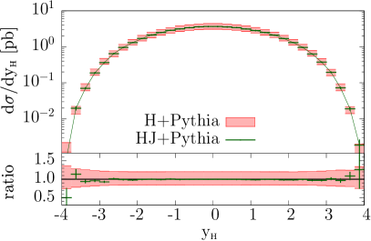
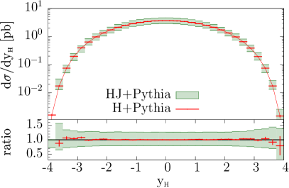
Refer to caption
Refer to caption
Figure 1: Comparison between the H+PYTHIA result and the HJ-MiNLO+PYTHIA result for the Higgs-boson rapidity distribution at the LHC at 8 TeV. The left plot shows the 7-point scale-variation band for the H generator, while the right plot shows the HJ-MiNLO 7-point band.

After having shown that the total cross sections obtained with the BJ-MiNLO generator are in good agreement with the standard NLO cross sections, we would like to show that also the rapidity distributions are in good agreement. We thus show in fig. 1 the rapidity distribution of the Higgs boson at the 8 TeV LHC, computed with the H and with the HJ-MiNLO generators, both interfaced to PYTHIA 6 [37] for shower. We have used the Perugia-0 tune of PYTHIA (that is to say, PYTUNE(320)). Hadronization, underlying event and multi-parton collisions were turned off. The two plots show the scale-variation band for each generator. The band is obtained as the upper and lower envelope of the results obtained by setting the scale factor parameters (KR,KF)subscript𝐾Rsubscript𝐾F(K_{\scriptscriptstyle\rm R},K_{\scriptscriptstyle\rm F}) to (1,1)11(1,1), (1,2)12(1,2), (2,1)21(2,1), (1,12)112(1,\frac{1}{2}), (12,1)121(\frac{1}{2},1), (12,12)1212(\frac{1}{2},\frac{1}{2}) and (2,2)22(2,2). We see considerable agreement between the two approaches, with the scale-variation band of the HJ-MiNLO result being slightly larger.
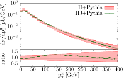
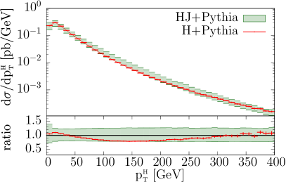
Refer to caption
Refer to caption
Figure 2: Comparison between the H+PYTHIA result and the HJ-MiNLO+PYTHIA result for the Higgs boson transverse-momentum distribution. The bands are obtained as in fig. 1.
Refer to caption
Refer to caption
Figure 3: Same as fig. 2 for a different pTHsuperscriptsubscript𝑝THp_{\mathchoice{\displaystyle}{\scriptstyle}{\scriptscriptstyle}{\scriptscriptstyle}\rm T}^{\rm\mathchoice{\displaystyle}{\scriptstyle}{\scriptscriptstyle}{\scriptscriptstyle}H} range.

In figs. 2 and 3 we show the Higgs transverse momentum distributions. We begin by noticing that the central values of the H and HJ-MiNLO generators are in very good agreement. This is not a surprise, since in the H generator, the parameter hfact, that separates the real cross section contribution into the sum of a singular and a finite one, was set to the value MH/1.2subscript𝑀𝐻1.2M_{\scriptscriptstyle H}/1.2, motivated by the fact that this yields better agreement with the NNLO result.

We notice that, for large transverse momenta, the HJ-MiNLO generator has a smaller scale variation band with respect to the H one. We expect this behaviour, since the HJ-MiNLO generator achieves NLO accuracy for one-jet inclusive distributions, while the H generator is only tree-level accurate. We also notice that the scale uncertainty band of HJ-MiNLO widens at small transverse momentum. This behaviour is also expected, since, in that direction, we approach the strong coupling regime. Observe also that the H result does not show a realistic scale uncertainty in the pTH<MHsuperscriptsubscript𝑝THsubscript𝑀𝐻p_{\mathchoice{\displaystyle}{\scriptstyle}{\scriptscriptstyle}{\scriptscriptstyle}\rm T}^{\mathchoice{\displaystyle}{\scriptstyle}{\scriptscriptstyle}{\scriptscriptstyle}\rm H}<M_{\scriptscriptstyle H} region. This too is understood, and it follows from the fact that this region is dominated by S𝑆S-type events (see refs. [36, 38] for a detailed explanation).

As a last point, we see from fig. 3, that a noticeable difference in shape is present in the very small transverse-momentum region. This again does not come as a surprise, since the POWHEG-generated Sudakov form factor in the H generator differs by NNLL terms, and also by non-singular contributions, from the HJ-MiNLO one. Notice also that, unlike in the H case [38], the scale variation in the HJ-MiNLO generator induces a change in shape of the transverse momentum spectrum in the Sudakov region, leading to a better understanding of the associated uncertainty.
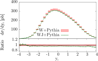
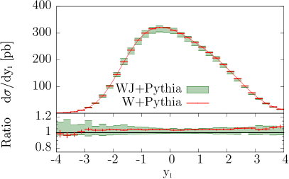
Refer to caption
Refer to caption
Figure 4: Comparison between the W+PYTHIA result and the WJ-MiNLO+PYTHIA result for the lsuperscript𝑙l^{-} rapidity distribution at the Tevatron. The bands are obtained as in fig. 1 for the W+PYTHIA generator, while for the WJ-MiNLO+PYTHIA generator they are obtained by taking the upper and lower envelope of the curves computed with KR=KF={1/2,1,2}subscript𝐾Rsubscript𝐾F1212K_{\scriptscriptstyle\rm R}=K_{\scriptscriptstyle\rm F}=\{1/2,1,2\}.

We now turn to the case of Wsuperscript𝑊W^{-} production. Motivated by the discussion given for the total cross section case, we consider only a 3-point scale variation, i.e. KR=KF={1/2,1,2}subscript𝐾Rsubscript𝐾F1212K_{\scriptscriptstyle\rm R}=K_{\scriptscriptstyle\rm F}=\{1/2,1,2\} for the WJ-MiNLO generator. In fig. 4 we show the lsuperscript𝑙l^{-} rapidity distribution at the Tevatron computed with the W and WJ+MiNLO generators. We essentially see no shape difference in this distribution, therefore, as for the inclusive cross section, we find that the WJ+MiNLO central value is about 5% below the W one. The WJ band is slightly larger than the W one for central rapidities, widening towards larger rapidities.
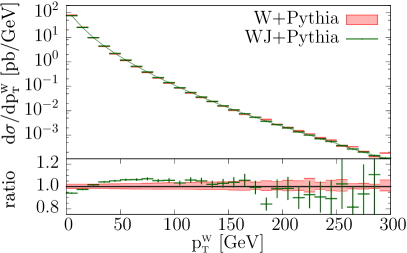
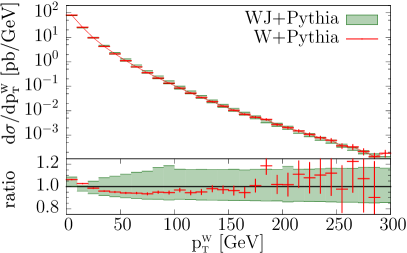
Refer to caption
Refer to caption
Figure 5: Comparison between the W+PYTHIA result and the WJ-MiNLO+PYTHIA result for the Wsuperscript𝑊W^{-} transverse-momentum distribution at the Tevatron. The bands are obtained as in fig. 4.
Refer to caption
Refer to caption
Figure 6: Same as fig. 5 for a different pTWsuperscriptsubscript𝑝TWp_{\mathchoice{\displaystyle}{\scriptstyle}{\scriptscriptstyle}{\scriptscriptstyle}\rm T}^{\rm\mathchoice{\displaystyle}{\scriptstyle}{\scriptscriptstyle}{\scriptscriptstyle}W} range.

In figs. 5 and 6 we present predictions for the Wsuperscript𝑊W^{-} boson transverse-momentum spectrum. In this case we find noticeable shape differences between the W and WJ+MiNLO distribution, especially at low pTWsuperscriptsubscript𝑝TWp_{\mathchoice{\displaystyle}{\scriptstyle}{\scriptscriptstyle}{\scriptscriptstyle}\rm T}^{\rm\mathchoice{\displaystyle}{\scriptstyle}{\scriptscriptstyle}{\scriptscriptstyle}W}. In particular, we observe that the WJ+MiNLO Sudakov form factor peaks at a lower value of pTWsuperscriptsubscript𝑝TWp_{\mathchoice{\displaystyle}{\scriptstyle}{\scriptscriptstyle}{\scriptscriptstyle}\rm T}^{\rm\mathchoice{\displaystyle}{\scriptstyle}{\scriptscriptstyle}{\scriptscriptstyle}W}. These differences do not come as a surprise, since this distribution is described only at LO by the W generator, while the WJ+MiNLO description is NLO accurate. We also note that the W uncertainty band is small and uniform in the whole pTWsuperscriptsubscript𝑝TWp_{\mathchoice{\displaystyle}{\scriptstyle}{\scriptscriptstyle}{\scriptscriptstyle}\rm T}^{\rm\mathchoice{\displaystyle}{\scriptstyle}{\scriptscriptstyle}{\scriptscriptstyle}W} range. This is a feature of POWHEG when no separation is performed between singular and regular contributions to the cross section. In this case, the size of the scale variation amounts to a factor 1+𝒪(αS2)1𝒪superscriptsubscript𝛼S21+{\cal O}(\alpha_{\mathchoice{\displaystyle}{\scriptstyle}{\scriptscriptstyle}{\scriptscriptstyle}\rm S}^{2}), that is clearly too small in the moderate to large pTWsuperscriptsubscript𝑝TWp_{\mathchoice{\displaystyle}{\scriptstyle}{\scriptscriptstyle}{\scriptscriptstyle}\rm T}^{\rm\mathchoice{\displaystyle}{\scriptstyle}{\scriptscriptstyle}{\scriptscriptstyle}W} region, where the W generator is only tree-level accurate. The error band given by the WJ+MiNLO generator is of an acceptable size at large transverse momenta, while it seems to be excessively small in the very low transverse momentum region.
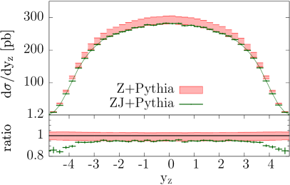
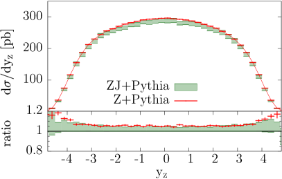
Refer to caption
Refer to caption
Figure 7: Comparison between the Z+PYTHIA result and the ZJ-MiNLO+PYTHIA result for the Z𝑍Z rapidity distribution at the LHC at 14 TeV. The bands are obtained as in fig. 4.

Finally, we discuss the case of Z𝑍Z production at the 14 TeV LHC. In fig. 7 we show the Z𝑍Z boson rapidity distribution. As in the case of W𝑊W production, we note that the ZJ+MiNLO central value is lower than the Z one and that its uncertainty band is comparable at central rapidities, widening in the forward-backward region. We also notice a slight change of shape in the extreme rapidities, with the Z result remaining compatible with the ZJ+MiNLO uncertainty band.
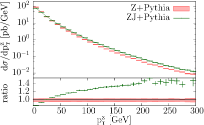
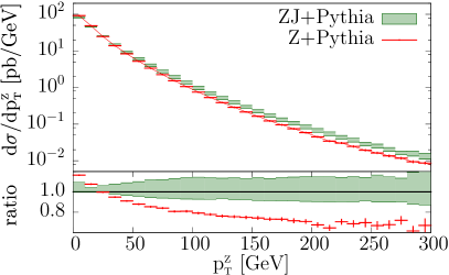
Refer to caption
Refer to caption
Figure 8: Comparison between the Z+PYTHIA result and the ZJ-MiNLO+PYTHIA result for the Z𝑍Z transverse-momentum distribution at the LHC at 14 TeV. The bands are obtained as in fig. 4.
Refer to caption
Refer to caption
Figure 9: Same as fig. 8 for a different pTZsuperscriptsubscript𝑝TZp_{\mathchoice{\displaystyle}{\scriptstyle}{\scriptscriptstyle}{\scriptscriptstyle}\rm T}^{\rm\mathchoice{\displaystyle}{\scriptstyle}{\scriptscriptstyle}{\scriptscriptstyle}Z} range.

In figs. 8 and 9 we show the transverse-momentum distribution of the Z𝑍Z boson. We notice the same features already observed in the W𝑊W case. However we also observe now a considerable difference of the Z and ZJ-MiNLO distributions at large transverse momenta. Following arguments in ref. [39] we suggest that this difference arises due to NLO corrections in the ZJ-MiNLO generator which are not present in the Z one, for example those related to threshold logarithms.

In conclusion, we have seen that in the case of vector-boson production (Z𝑍Z and W𝑊W), the agreement of the BJ-MiNLO and the B generators is less than perfect. We also have shown that there is not a close correspondence between the scale variations in the two types of generators. We may conclude from this observation that either the scale variation in the MiNLO generator is excessive, and should be limited (for example by considering only 3-point scale variations), or that the scale uncertainty obtained in the W and Z generators underestimates the true error. We also remark that if we use the full 7-point scale variation for the WJ and ZJ generators, the error bands for the transverse-momentum distributions do not shrink as much at small transverse momenta, thus leading to better compatibility with the W and Z generators distributions. On the other hand, by doing so, the error on the total cross section might be too conservative. The problems with the application of our method to these generators may be related to the fact that the bulk of the Sudakov region is relatively low, the peak being below 5 GeV. We have ignored some problems that may be relevant in this region. For example, the pdf evolution switches from 5 to 4 and to 3 flavours in this region, while we have used constant nf=5subscript𝑛𝑓5n_{f}=5 in the BJ-MiNLO generator. Similarly, inaccuracies in the pdf evolution in this region may also be relevant. While we have checked that our results are not affected in a relevant way by the infrared cutoffs of the calculation, we believe that further work will be needed to better assess the importance of low-pTsubscript𝑝Tp_{\mathchoice{\displaystyle}{\scriptstyle}{\scriptscriptstyle}{\scriptscriptstyle}\rm T} Sudakov region.

On the contrary, in the Higgs boson case, we find from our study a fairly good agreement between the H and HJ-MiNLO generators, both for the total cross sections and for the distributions. The scale variation bands are also comparable, which confirms that our result yields an improved and more accurate description of Higgs boson production, fulfilling also, in a practical, way our goals.

5 How to build an NNLO+PS generator with MiNLO

We argue now that a generator built according to the MiNLO prescription, improved with the findings of the present work, can be easily turned into an NNLO+PS generator. For the sake of simplicity, we consider the Higgs boson generator. We have concluded that such a simulation achieves 𝒪(αS4)𝒪superscriptsubscript𝛼S4{\cal O}(\alpha_{\mathchoice{\displaystyle}{\scriptstyle}{\scriptscriptstyle}{\scriptscriptstyle}\rm S}^{4}) accuracy for all distributions involving at least one jet and 𝒪(αS3)𝒪superscriptsubscript𝛼S3{\cal O}(\alpha_{\mathchoice{\displaystyle}{\scriptstyle}{\scriptscriptstyle}{\scriptscriptstyle}\rm S}^{3}) accuracy for inclusive distributions. We denote by

(dσdy)HJsubscriptd𝜎d𝑦HJ\left(\frac{\mathrm{d}\sigma}{\mathrm{d}y}\right)_{\mbox{{\tt HJ}{}}} (48)

the inclusive Higgs boson rapidity distribution obtained with this event generator. We denote by

(dσdy)NNLOsubscriptd𝜎d𝑦NNLO\left(\frac{\mathrm{d}\sigma}{\mathrm{d}y}\right)_{\mbox{\scriptsize{NNLO}}} (49)

the inclusive Higgs boson rapidity distribution calculated with a fixed NNLO calculation. We claim that by reweighting the HJ-MiNLO output with the weight factor

(dσdy)NNLO(dσdy)HJsubscriptd𝜎d𝑦NNLOsubscriptd𝜎d𝑦HJ\frac{\left(\frac{\mathrm{d}\sigma}{\mathrm{d}y}\right)_{\mbox{\scriptsize{NNLO}}}}{\left(\frac{\mathrm{d}\sigma}{\mathrm{d}y}\right)_{\mbox{{\tt HJ}{}}}} (50)

we achieve full NNLO accuracy for our generator. The proof is simple. The above ratio has a formal expansion

(dσdy)NNLO(dσdy)HJ=c2αS2+c3αS3+c4αS4c2αS2+c3αS3+d4αS41+c4d4c2αS2+𝒪(αS3).subscriptd𝜎d𝑦NNLOsubscriptd𝜎d𝑦HJsubscript𝑐2superscriptsubscript𝛼S2subscript𝑐3superscriptsubscript𝛼S3subscript𝑐4superscriptsubscript𝛼S4subscript𝑐2superscriptsubscript𝛼S2subscript𝑐3superscriptsubscript𝛼S3subscript𝑑4superscriptsubscript𝛼S41subscript𝑐4subscript𝑑4subscript𝑐2superscriptsubscript𝛼S2𝒪superscriptsubscript𝛼S3\frac{\left(\frac{\mathrm{d}\sigma}{\mathrm{d}y}\right)_{\mbox{\scriptsize{NNLO}}}}{\left(\frac{\mathrm{d}\sigma}{\mathrm{d}y}\right)_{\mbox{{\tt HJ}{}}}}=\frac{c_{2}\alpha_{\mathchoice{\displaystyle}{\scriptstyle}{\scriptscriptstyle}{\scriptscriptstyle}\rm S}^{2}+c_{3}\alpha_{\mathchoice{\displaystyle}{\scriptstyle}{\scriptscriptstyle}{\scriptscriptstyle}\rm S}^{3}+c_{4}\alpha_{\mathchoice{\displaystyle}{\scriptstyle}{\scriptscriptstyle}{\scriptscriptstyle}\rm S}^{4}}{c_{2}\alpha_{\mathchoice{\displaystyle}{\scriptstyle}{\scriptscriptstyle}{\scriptscriptstyle}\rm S}^{2}+c_{3}\alpha_{\mathchoice{\displaystyle}{\scriptstyle}{\scriptscriptstyle}{\scriptscriptstyle}\rm S}^{3}+d_{4}\alpha_{\mathchoice{\displaystyle}{\scriptstyle}{\scriptscriptstyle}{\scriptscriptstyle}\rm S}^{4}}\approx 1+\frac{c_{4}-d_{4}}{c_{2}}\alpha_{\mathchoice{\displaystyle}{\scriptstyle}{\scriptscriptstyle}{\scriptscriptstyle}\rm S}^{2}+{\cal O}(\alpha_{\mathchoice{\displaystyle}{\scriptstyle}{\scriptscriptstyle}{\scriptscriptstyle}\rm S}^{3}). (51)

Notice that the numerator and denominator agree at 𝒪(αS3)𝒪superscriptsubscript𝛼S3{\cal O}(\alpha_{\mathchoice{\displaystyle}{\scriptstyle}{\scriptscriptstyle}{\scriptscriptstyle}\rm S}^{3}) since the HJ-MiNLO generator achieves 𝒪(αS3)𝒪superscriptsubscript𝛼S3{\cal O}(\alpha_{\mathchoice{\displaystyle}{\scriptstyle}{\scriptscriptstyle}{\scriptscriptstyle}\rm S}^{3}) accuracy for inclusive observables. Thus, the reweighting factor does not spoil the αS4superscriptsubscript𝛼S4\alpha_{\mathchoice{\displaystyle}{\scriptstyle}{\scriptscriptstyle}{\scriptscriptstyle}\rm S}^{4} accuracy of the HJ-MiNLO generator in the one-jet region. In this region, in fact, the dominant contributions to the HJ-MiNLO generator are of order αS3superscriptsubscript𝛼S3\alpha_{\mathchoice{\displaystyle}{\scriptstyle}{\scriptscriptstyle}{\scriptscriptstyle}\rm S}^{3}, and the reweighting generates extra contributions of order αS5superscriptsubscript𝛼S5\alpha_{\mathchoice{\displaystyle}{\scriptstyle}{\scriptscriptstyle}{\scriptscriptstyle}\rm S}^{5}, that are beyond the nominal accuracy. On the other hand, the inclusive distributions are reweighted to achieve αS4superscriptsubscript𝛼S4\alpha_{\mathchoice{\displaystyle}{\scriptstyle}{\scriptscriptstyle}{\scriptscriptstyle}\rm S}^{4} accuracy, so that the generator has indeed αS4superscriptsubscript𝛼S4\alpha_{\mathchoice{\displaystyle}{\scriptstyle}{\scriptscriptstyle}{\scriptscriptstyle}\rm S}^{4} accuracy in the whole phase space.

Variants of these schemes are also possible. Rather than reweighting using the full rapidity distribution, one can split the cross section as

d2σdqTdy=d2σdqTdyh(qT)+d2σdqTdy[1h(qT)],superscriptd2𝜎dsubscript𝑞Td𝑦superscriptd2𝜎dsubscript𝑞Td𝑦subscript𝑞Tsuperscriptd2𝜎dsubscript𝑞Td𝑦delimited-[]1subscript𝑞T\frac{\mathrm{d}^{2}\sigma}{\mathrm{d}{q_{\mathchoice{\displaystyle}{\scriptstyle}{\scriptscriptstyle}{\scriptscriptstyle}\rm T}}\mathrm{d}y}=\frac{\mathrm{d}^{2}\sigma}{\mathrm{d}{q_{\mathchoice{\displaystyle}{\scriptstyle}{\scriptscriptstyle}{\scriptscriptstyle}\rm T}}\mathrm{d}y}\,h\left(q_{\mathchoice{\displaystyle}{\scriptstyle}{\scriptscriptstyle}{\scriptscriptstyle}\rm T}\right)+\frac{\mathrm{d}^{2}\sigma}{\mathrm{d}{q_{\mathchoice{\displaystyle}{\scriptstyle}{\scriptscriptstyle}{\scriptscriptstyle}\rm T}}\mathrm{d}y}\left[1-h\left(q_{\mathchoice{\displaystyle}{\scriptstyle}{\scriptscriptstyle}{\scriptscriptstyle}\rm T}\right)\right]\,, (52)

where hh is a smooth positive function such that h(qT)1subscript𝑞T1h(q_{\mathchoice{\displaystyle}{\scriptstyle}{\scriptscriptstyle}{\scriptscriptstyle}\rm T})\to 1 as qT0subscript𝑞T0q_{\mathchoice{\displaystyle}{\scriptstyle}{\scriptscriptstyle}{\scriptscriptstyle}\rm T}\to 0 and h(qT)0subscript𝑞T0h(q_{\mathchoice{\displaystyle}{\scriptstyle}{\scriptscriptstyle}{\scriptscriptstyle}\rm T})\to 0 for qTMHmuch-greater-thansubscript𝑞Tsubscript𝑀𝐻q_{\mathchoice{\displaystyle}{\scriptstyle}{\scriptscriptstyle}{\scriptscriptstyle}\rm T}\gg M_{\scriptscriptstyle H}, such as

h(q)=cMHαcMHα+qα,𝑞𝑐superscriptsubscript𝑀𝐻𝛼𝑐superscriptsubscript𝑀𝐻𝛼superscript𝑞𝛼h(q)=\frac{c\,M_{\scriptscriptstyle H}^{\alpha}}{c\,M_{\scriptscriptstyle H}^{\alpha}+q^{\alpha}}, (53)

with α1𝛼1\alpha\geq 1 and c𝑐c a constant of order 1. One can then reweight the cross section as

d2σdqTdyh(qT)W(y)+d2σdqTdy[1h(qT)],superscriptd2𝜎dsubscript𝑞Td𝑦subscript𝑞T𝑊𝑦superscriptd2𝜎dsubscript𝑞Td𝑦delimited-[]1subscript𝑞T\frac{\mathrm{d}^{2}\sigma}{\mathrm{d}{q_{\mathchoice{\displaystyle}{\scriptstyle}{\scriptscriptstyle}{\scriptscriptstyle}\rm T}}\mathrm{d}y}\,h\left(q_{\mathchoice{\displaystyle}{\scriptstyle}{\scriptscriptstyle}{\scriptscriptstyle}\rm T}\right)W\left(y\right)+\frac{\mathrm{d}^{2}\sigma}{\mathrm{d}{q_{\mathchoice{\displaystyle}{\scriptstyle}{\scriptscriptstyle}{\scriptscriptstyle}\rm T}}\mathrm{d}y}\left[1-h\left(q_{\mathchoice{\displaystyle}{\scriptstyle}{\scriptscriptstyle}{\scriptscriptstyle}\rm T}\right)\right]\,, (54)

with

W(y)=dqTh(qT)(d2σdqTdy)NNLOdqTh(qT)(d2σdqTdy)𝙷𝙹.𝑊𝑦differential-dsubscript𝑞Tsubscript𝑞Tsubscriptsuperscriptd2𝜎dsubscript𝑞Td𝑦NNLOdifferential-dsubscript𝑞Tsubscript𝑞Tsubscriptsuperscriptd2𝜎dsubscript𝑞Td𝑦𝙷𝙹W(y)=\frac{\displaystyle\int\mathrm{d}q_{\mathchoice{\displaystyle}{\scriptstyle}{\scriptscriptstyle}{\scriptscriptstyle}\rm T}\,h\left(q_{\mathchoice{\displaystyle}{\scriptstyle}{\scriptscriptstyle}{\scriptscriptstyle}\rm T}\right)\left(\frac{\mathrm{d}^{2}\sigma}{\mathrm{d}q_{\mathchoice{\displaystyle}{\scriptstyle}{\scriptscriptstyle}{\scriptscriptstyle}\rm T}\mathrm{d}y}\right)_{\mbox{\scriptsize{NNLO}}}}{\displaystyle\int\mathrm{d}q_{\mathchoice{\displaystyle}{\scriptstyle}{\scriptscriptstyle}{\scriptscriptstyle}\rm T}\,h\left(q_{\mathchoice{\displaystyle}{\scriptstyle}{\scriptscriptstyle}{\scriptscriptstyle}\rm T}\right)\left(\frac{\mathrm{d}^{2}\sigma}{\mathrm{d}q_{\mathchoice{\displaystyle}{\scriptstyle}{\scriptscriptstyle}{\scriptscriptstyle}\rm T}\mathrm{d}y}\right)_{{\tt HJ}{}}}\,. (55)

In this way, for qTMHmuch-greater-thansubscript𝑞Tsubscript𝑀𝐻q_{\mathchoice{\displaystyle}{\scriptstyle}{\scriptscriptstyle}{\scriptscriptstyle}\rm T}\gg M_{\scriptscriptstyle H} the effect of the reweighting vanishes.

We notice that this NNLO+PS generator would be NNLO accurate in the same sense in which the current MC@NLO or POWHEG type generators are NLO accurate, i.e. integrated quantities achieve NLO/NNLO accuracy, while LL/NLL/NNLL accuracy is achieved in the Sudakov region, depending upon the accuracy of the implementation of the Sudakov form factors.

We postpone a phenomenological study including reweighting to a future publication.

There are a number of more complex processes to which this procedure can be generalized, typically processes where the heavy particle decays, or processes involving pair production of massive colourless objects. In this case, the NNLO reweighting must be performed as a function of more variables. One would typically use the rapidity of the heavy system, plus the kinematical variables describing its internal structure. For example, one can go to the longitudinal rest frame of the heavy system with a Lorentz boost, perform a transverse boost of the system such that its transverse momentum vanishes, and use variables that describe the kinematics of the heavy system in this frame.

6 MiNLO merging for more complex processes

In the present work, we have dealt with relatively simple processes, i.e. a colour-neutral massive particle in association with one jet. The results of ref. [14] strongly suggest that our procedure may be generalized to higher jet multiplicities. Since, at the level of one associated jet, we had to improve the MiNLO prescription with the inclusion of certain NNLL terms in the Sudakov form factor, it is clear that, in general, we need to find a similar improvement for the more general case.

A first question that we would like to consider is whether our MiNLO procedure downgraded to the LO level (that is to say, to the CKKW procedure [40] as applied to the inclusive sample), already achieves our goal at LO accuracy, that is to say, it is such that by integrating the softest emission one gets a LO accurate matrix element for one less emission. It is easy to convince ourselves that as soon as we deal with matrix elements involving more than four coloured particles (including the softest emission), this is not the case. In fact, after the first clustering, that in our procedure simply sets the Q0subscript𝑄0Q_{0} scale, we are left with four or more coloured partons. Soft gluon resummation, in this case, also involve soft, non-collinear terms that arise from interference of the emission from the coloured external lines [41, 42, 43]. These terms are of NLL accuracy, and, according to our counting, they can contribute terms of relative order αSsubscript𝛼S\sqrt{\alpha_{\mathchoice{\displaystyle}{\scriptstyle}{\scriptscriptstyle}{\scriptscriptstyle}\rm S}}. By not including them, we thus introduce an error of this magnitude, while LO accuracy requires the neglected terms to be of order αSsubscript𝛼S\alpha_{\mathchoice{\displaystyle}{\scriptstyle}{\scriptscriptstyle}{\scriptscriptstyle}\rm S}. Notice that this problem does not manifest itself in the HJJ case, since precisely four coloured partons are present here (two in the initial state and two in the final state). In processes like tt¯𝑡¯𝑡t\bar{t} production in association with one jet, such terms would have to be accounted for. On the other hand, it is possible to compute these terms using standard resummation techniques. It is thus conceivable that the LO MiNLO formula can also be improved including these interference terms. But we also stress that the CKKW procedure, as is, does not satisfy our requirement at leading order.

In the present work, we have used as a clustering variable the transverse momentum of the boson, since it is a simple variable and the corresponding resummation formulae are well known. As an alternative, we could have used the hardest jet transverse momentum, taking B2subscript𝐵2B_{2} from ref. [44]. If this method is to be extended to processes with more than one radiated parton, it is clear that other clustering variables should be chosen, likely with good resummation properties. One should then seek either an NNLL extension of the CKKW procedure, or, construct a product of standard soft resummation factors, accurate at the NLL level, modifying the Sudakov form factor in each one to include the B2subscript𝐵2B_{2} term relevant to the associated configuration of clustered particles. Notice that within our method it was never necessary to know explicitly the hard resummation correction that is usually included in NLL and NNLL resummation formulae, since the NLO matrix elements intrinsically provide this.

7 Conclusions

In the present work, we have illustrated a method for constructing NLO+PS generators for the production of a heavy system accompanied by a radiated parton, such that, when integrating over the parton’s phase space, one recovers the accuracy of a corresponding NLO+PS generator for the production of the heavy system alone. In essence, in our method, we start from the MiNLO prescription of ref. [14], and we look explicitly for the places in which it needs to be modified in order to maintain NLO accuracy on integrating out all radiation. We have found that the inclusion of the A2subscript𝐴2A_{2} and the B2subscript𝐵2B_{2} term in the resummation formula is enough to achieve this goal. Since we do not know the B2subscript𝐵2B_{2} term for the type of clustering that we performed in ref. [14], we have modified the prescription so that the transverse momentum of the boson is used instead. More specifically, the prescription is applicable to any clustering scheme in which the last step is performed using the transverse momentum of the boson as the clustering scale.

We have not explored, at this moment, any issues related to the logarithmic accuracy of our approach. In other words, the logarithmic accuracy should be at the same level as that of the NLO+PS generators we are referring to. We postpone to future studies, a more accurate assessment of, and possible improvements to, the precision of the resummation.

We have tested our method in the framework of H/W/Z production. We find that the method performs remarkably well. We have also found that the usual scale-variation method used in order to determine uncertainties may be deceiving in our case, especially for processes like W/Z production, where, at the Born level, there is no renormalization scale dependence. We track this problem to the fact that, in the corresponding BJ calculation, a renormalization scale variation is already possible at the Born level.

We point out that, using our BJ-MiNLO generators, it is actually possible to construct an NNLO+PS generator, simply by reweighting the transverse-momentum integral of the cross section to the one computed at the NNLO level. We postpone a phenomenological study of this method to a future publication.

While this work was under completion, a publication has appeared that has some points in common with our work [11]. This work focuses on the accuracy of the matching conditions, and sets up a framework, using NNLL accurate resummation of soft-parton emission, such that one has no loss of NLO accuracy when matching. Also our approach is motivated by the requirement of preserving the NLO accuracy. It is more focussed, however, upon finding the minimal modification to the soft-parton resummation such that no matching is needed at all, and, in fact, we identify precisely where do we need to improve the resummation formula in order to achieve our goal. In this way, we find that its implementation in the BJ case requires only a minimal modification to the MiNLO procedure, that, by itself, is quite simple.

Acknowledgments

We thank Gavin Salam and Massimiliano Grazzini for useful discussions. G.Z. is supported by the British Science and Technology Facilities Council. G.Z., P.N. and C.O. acknowledge the support also of grant PITN-GA-2010-264564 from the European Commission.

Appendix A The NNLL resummed differential cross section

The NNLL differential cross section for the production of a colourless system, denoted by B𝐵B, of virtuality Q2superscript𝑄2Q^{2} (when dealing with a single vector boson, we assume that Q𝑄Q is equal to the vector boson mass M𝑀M), in the partonic scattering i+jB𝑖𝑗𝐵i+j\to B, is given by

dσdqT2dyB=σ0d2beiqTb[Ciafa/A](xA,c1b)[Cjbfb/B](xB,c1b)×exp𝒮(c2Q,c1b),d𝜎dsuperscriptsubscript𝑞T2dsubscript𝑦Bsubscript𝜎0superscriptd2𝑏superscript𝑒𝑖subscript𝑞T𝑏delimited-[]tensor-productsubscript𝐶𝑖𝑎subscript𝑓𝑎𝐴subscript𝑥𝐴subscript𝑐1𝑏delimited-[]tensor-productsubscript𝐶𝑗𝑏subscript𝑓𝑏𝐵subscript𝑥Bsubscript𝑐1𝑏𝒮subscript𝑐2𝑄subscript𝑐1𝑏\frac{\mathrm{d}\sigma}{\mathrm{d}q_{\mathchoice{\displaystyle}{\scriptstyle}{\scriptscriptstyle}{\scriptscriptstyle}\rm T}^{2}\mathrm{d}y_{\rm\scriptscriptstyle B}}=\sigma_{0}\!\int\!\mathrm{d}^{2}b\,e^{i\vec{q}_{\mathchoice{\displaystyle}{\scriptstyle}{\scriptscriptstyle}{\scriptscriptstyle}\rm T}\cdot\vec{b}}\left[C_{ia}\otimes f_{a/A}\right]\!\left(x_{A},\frac{c_{1}}{b}\right)\left[C_{jb}\otimes f_{b/B}\right]\!\left(x_{\mathrm{B}},\frac{c_{1}}{b}\right)\times\exp{\cal S}\left(c_{2}Q,\frac{c_{1}}{b}\right), (56)

where we have used the following definition of convolution

[Cijfj/J](x,q)x1dξξfi/J(ξ,q)Cij(αS(q2),xξ).delimited-[]tensor-productsubscript𝐶𝑖𝑗subscript𝑓𝑗𝐽𝑥𝑞superscriptsubscript𝑥1d𝜉𝜉subscript𝑓𝑖𝐽𝜉𝑞subscript𝐶𝑖𝑗subscript𝛼Ssuperscript𝑞2𝑥𝜉\left[C_{ij}\otimes f_{j/J}\right]\!\left(x,q\right)\equiv\int_{x}^{1}\frac{\mathrm{d}\xi}{\xi}\,f_{i/J}\left(\xi,q\right)C_{ij}\left(\alpha_{\mathchoice{\displaystyle}{\scriptstyle}{\scriptscriptstyle}{\scriptscriptstyle}\rm S}\left(q^{2}\right),\frac{x}{\xi}\right). (57)

The σ0subscript𝜎0\sigma_{0} factor is such that, at leading order,

(dσdyB)LO=fi/A(xA,μF)fj/B(xB,μF)σ0,subscriptd𝜎dsubscript𝑦BLOsubscript𝑓𝑖𝐴subscript𝑥𝐴subscript𝜇𝐹subscript𝑓𝑗Bsubscript𝑥Bsubscript𝜇𝐹subscript𝜎0\left(\frac{\mathrm{d}\sigma}{\mathrm{d}y_{\rm\scriptscriptstyle B}}\right)_{\rm LO}=f_{i/A}\left(x_{A},\mu_{F}\right)f_{j/\mathrm{B}}\left(x_{\mathrm{B}},\mu_{F}\right)\sigma_{0}\,, (58)

and the rapidity of the B𝐵B system is given by

yB=12logxAxB.subscript𝑦B12subscript𝑥𝐴subscript𝑥𝐵y_{\rm\scriptscriptstyle B}=\frac{1}{2}\log\frac{x_{A}}{x_{B}}\,. (59)

The Sudakov form factor 𝒮(q,q)𝒮superscript𝑞𝑞\mathcal{S}\left(q^{\prime},q\right) is defined by 777Note that this Sudakov is the square of the Sudakov form factor Δq/gsubscriptΔ𝑞𝑔\Delta_{q/g} considered in Sec. 2 (see eq. 12). Therefore the coefficients Aisubscript𝐴𝑖A_{i} and Bisubscript𝐵𝑖B_{i} here are twice those given in eqs. (5) and (6).

𝒮(q,q)=q2q2dμ2μ2[A(αS(μ2))logq2μ2+B(αS(μ2))],𝒮superscript𝑞𝑞superscriptsubscriptsuperscript𝑞2superscript𝑞2dsuperscript𝜇2superscript𝜇2delimited-[]𝐴subscript𝛼Ssuperscript𝜇2superscript𝑞2superscript𝜇2𝐵subscript𝛼Ssuperscript𝜇2\mathcal{S}\left(q^{\prime},q\right)=-\int_{q^{2}}^{q^{\prime 2}}\frac{\mathrm{d}\mu^{2}}{\mu^{2}}\left[A\left(\alpha_{\mathchoice{\displaystyle}{\scriptstyle}{\scriptscriptstyle}{\scriptscriptstyle}\rm S}\left(\mu^{2}\right)\right)\log\frac{q^{\prime 2}}{\mu^{2}}+B\left(\alpha_{\mathchoice{\displaystyle}{\scriptstyle}{\scriptscriptstyle}{\scriptscriptstyle}\rm S}\left(\mu^{2}\right)\right)\right], (60)

and the Cijsubscript𝐶𝑖𝑗C_{ij} coefficients have the following perturbative expansion

CijCij(αS,z)=δijδ(1z)+αSCij(1)(z)+subscript𝐶𝑖𝑗subscript𝐶𝑖𝑗subscript𝛼S𝑧subscript𝛿𝑖𝑗𝛿1𝑧subscript𝛼Ssuperscriptsubscript𝐶𝑖𝑗1𝑧C_{ij}\equiv C_{ij}\left(\alpha_{\mathchoice{\displaystyle}{\scriptstyle}{\scriptscriptstyle}{\scriptscriptstyle}\rm S},z\right)=\delta_{ij}\delta\left(1-z\right)+\alpha_{\mathchoice{\displaystyle}{\scriptstyle}{\scriptscriptstyle}{\scriptscriptstyle}\rm S}\,C_{ij}^{(1)}\left(z\right)+\ldots (61)

The Cijsubscript𝐶𝑖𝑗C_{ij} functions can thus be absorbed into a redefinition of the pdfs. We will thus assume now that our pdfs include this factor, and only at the end we will reinstate it.

Equation (56) is easily manipulated by going to Mellin space. However, we do not want to lose the information on the rapidity yBsubscript𝑦By_{\rm\scriptscriptstyle B} of the B𝐵B system. We then define the following Fourier-Mellin transform

σNdτdyBτα1ei 2βyBdσdqT2dyBsubscript𝜎𝑁differential-d𝜏differential-dsubscript𝑦Bsuperscript𝜏𝛼1superscript𝑒𝑖2𝛽subscript𝑦Bd𝜎dsuperscriptsubscript𝑞T2dsubscript𝑦B\sigma_{N}\equiv\int\mathrm{d}\tau\,\mathrm{d}y_{\rm\scriptscriptstyle B}\,\tau^{\alpha-1}\,e^{i\,2\,\beta\,y_{\rm\scriptscriptstyle B}}\frac{\mathrm{d}\sigma}{\mathrm{d}q_{\mathchoice{\displaystyle}{\scriptstyle}{\scriptscriptstyle}{\scriptscriptstyle}\rm T}^{2}\mathrm{d}y_{\rm\scriptscriptstyle B}} (62)

where

τ=xAxB,𝜏subscript𝑥𝐴subscript𝑥𝐵\tau=x_{A}x_{B}\,, (63)

so that S=Q2/τ𝑆superscript𝑄2𝜏S=Q^{2}/\tau, where S𝑆S is the hadronic center-of-mass energy. Notice that the τ𝜏\tau integration is performed by considering that S𝑆S goes from Q2superscript𝑄2Q^{2} to infinity. We can then introduce a complex number N𝑁N such that N=α+iβ𝑁𝛼𝑖𝛽N=\alpha+i\,\beta, so that we can write

σNsubscript𝜎𝑁\displaystyle\sigma_{N} =\displaystyle= 01dxAdxBτRe[N]1ei 2Im[N]yBdσdqT2dyBsuperscriptsubscript01differential-dsubscript𝑥𝐴differential-dsubscript𝑥𝐵superscript𝜏Redelimited-[]𝑁1superscript𝑒𝑖2Imdelimited-[]𝑁subscript𝑦Bd𝜎dsuperscriptsubscript𝑞T2dsubscript𝑦B\displaystyle\int_{0}^{1}\mathrm{d}x_{A}\,\mathrm{d}x_{B}\,\tau^{{\rm Re}\left[N\right]-1}\,e^{i\,2\,{\rm Im}\left[N\right]\,y_{\rm\scriptscriptstyle B}}\frac{\mathrm{d}\sigma}{\mathrm{d}q_{\mathchoice{\displaystyle}{\scriptstyle}{\scriptscriptstyle}{\scriptscriptstyle}\rm T}^{2}\mathrm{d}y_{\rm\scriptscriptstyle B}} (64)
=\displaystyle= 01dxAdxB(xAxB)Re[N]1(xAxB)iIm[N]dσdqT2dyBsuperscriptsubscript01differential-dsubscript𝑥𝐴differential-dsubscript𝑥𝐵superscriptsubscript𝑥𝐴subscript𝑥𝐵Redelimited-[]𝑁1superscriptsubscript𝑥𝐴subscript𝑥𝐵𝑖Imdelimited-[]𝑁d𝜎dsuperscriptsubscript𝑞T2dsubscript𝑦B\displaystyle\int_{0}^{1}\mathrm{d}x_{A}\,\mathrm{d}x_{B}\,\left(x_{A}x_{B}\right)^{{\rm Re}\left[N\right]-1}\left(\frac{x_{A}}{x_{B}}\right)^{i{\rm Im}\left[N\right]}\frac{\mathrm{d}\sigma}{\mathrm{d}q_{\mathchoice{\displaystyle}{\scriptstyle}{\scriptscriptstyle}{\scriptscriptstyle}\rm T}^{2}\mathrm{d}y_{\rm\scriptscriptstyle B}}
=\displaystyle= 01dxAdxBxAxBxANxBNdσdqT2dyBsuperscriptsubscript01dsubscript𝑥𝐴dsubscript𝑥𝐵subscript𝑥𝐴subscript𝑥𝐵superscriptsubscript𝑥𝐴𝑁superscriptsubscript𝑥𝐵superscript𝑁d𝜎dsuperscriptsubscript𝑞T2dsubscript𝑦B\displaystyle\int_{0}^{1}\frac{\mathrm{d}x_{A}\,\mathrm{d}x_{B}}{x_{A}\,x_{B}}\,x_{A}^{N}\,x_{B}^{N^{\ast}}\frac{\mathrm{d}\sigma}{\mathrm{d}q_{\mathchoice{\displaystyle}{\scriptstyle}{\scriptscriptstyle}{\scriptscriptstyle}\rm T}^{2}\mathrm{d}y_{\rm\scriptscriptstyle B}}
=\displaystyle= σ0d2beiqTbfa/A,N(c1b)fb/B,N(c1b)exp𝒮(c2Q,c1b),subscript𝜎0superscriptd2𝑏superscript𝑒𝑖subscript𝑞T𝑏subscript𝑓𝑎𝐴𝑁subscript𝑐1𝑏subscript𝑓𝑏𝐵superscript𝑁subscript𝑐1𝑏𝒮subscript𝑐2𝑄subscript𝑐1𝑏\displaystyle\sigma_{0}\int\mathrm{d}^{2}b\,e^{i\vec{q}_{\mathchoice{\displaystyle}{\scriptstyle}{\scriptscriptstyle}{\scriptscriptstyle}\rm T}\cdot\vec{b}}\,f_{a/A,N}\left(\frac{c_{1}}{b}\right)\,f_{b/B,N^{\ast}}\left(\frac{c_{1}}{b}\right)\,\exp\mathcal{S}\left(c_{2}Q,\frac{c_{1}}{b}\right),

with

fa/A,N(c1b)=01dxAxAN1fa/A(xA,c1b).subscript𝑓𝑎𝐴𝑁subscript𝑐1𝑏superscriptsubscript01differential-dsubscript𝑥𝐴superscriptsubscript𝑥𝐴𝑁1subscript𝑓𝑎𝐴subscript𝑥𝐴subscript𝑐1𝑏f_{a/A,N}\left(\frac{c_{1}}{b}\right)=\int_{0}^{1}{\mathrm{d}x_{A}}\,x_{A}^{N-1}f_{a/A}(x_{A},\frac{c_{1}}{b})\,. (65)

By solving the DGLAP equations for the pdfs to the required logarithmic accuracy, and evolving the moments of the Cijsubscript𝐶𝑖𝑗C_{ij} coefficients too, we can write

fa/A,N(c1b)fb/B,N(c1b)subscript𝑓𝑎𝐴𝑁subscript𝑐1𝑏subscript𝑓𝑏𝐵superscript𝑁subscript𝑐1𝑏\displaystyle f_{a/A,N}\left(\frac{c_{1}}{b}\right)\,f_{b/B,N^{\ast}}\left(\frac{c_{1}}{b}\right) =\displaystyle= fa/A,N(c2Q)fb/B,N(c2Q)exp{Re[𝒢N(c2Q,c1b)]}subscript𝑓𝑎𝐴𝑁subscript𝑐2𝑄subscript𝑓𝑏𝐵superscript𝑁subscript𝑐2𝑄Redelimited-[]subscript𝒢𝑁subscript𝑐2𝑄subscript𝑐1𝑏\displaystyle f_{a/A,N}\left(c_{2}Q\right)\,f_{b/B,N^{\ast}}\left(c_{2}Q\right)\,\exp\left\{{\rm Re}\left[{\cal G}_{N}\left(c_{2}Q,\frac{c_{1}}{b}\right)\right]\right\} (66)
\displaystyle\equiv FN(c2Q)exp{Re[𝒢N(c2Q,c1b)]},subscript𝐹𝑁subscript𝑐2𝑄Redelimited-[]subscript𝒢𝑁subscript𝑐2𝑄subscript𝑐1𝑏\displaystyle F_{N}(c_{2}Q)\,\exp\left\{{\rm Re}\left[{\cal G}_{N}\left(c_{2}Q,\frac{c_{1}}{b}\right)\right]\right\},

with (see eq. (2.22) of ref. [18])

𝒢N(c2Q,c1b)=2c12/b2c22Q2dμ2μ2γN(αS(μ2)).subscript𝒢𝑁subscript𝑐2𝑄subscript𝑐1𝑏2superscriptsubscriptsuperscriptsubscript𝑐12superscript𝑏2superscriptsubscript𝑐22superscript𝑄2dsuperscript𝜇2superscript𝜇2subscript𝛾𝑁subscript𝛼Ssuperscript𝜇2\mathcal{G}_{N}\left(c_{2}Q,\frac{c_{1}}{b}\right)=-2\int_{c_{1}^{2}/b^{2}}^{c_{2}^{2}Q^{2}}\frac{\mathrm{d}\mu^{2}}{\mu^{2}}\,\gamma_{N}\left(\alpha_{\mathchoice{\displaystyle}{\scriptstyle}{\scriptscriptstyle}{\scriptscriptstyle}\rm S}\left(\mu^{2}\right)\right). (67)

We define

αSsubscript𝛼S\displaystyle\alpha_{\mathchoice{\displaystyle}{\scriptstyle}{\scriptscriptstyle}{\scriptscriptstyle}\rm S} =\displaystyle= αS(c22Q2),subscript𝛼Ssuperscriptsubscript𝑐22superscript𝑄2\displaystyle\alpha_{\mathchoice{\displaystyle}{\scriptstyle}{\scriptscriptstyle}{\scriptscriptstyle}\rm S}\left(c_{2}^{2}Q^{2}\right)\,, (68)
y𝑦\displaystyle y =\displaystyle= αSb0logc12c22b2Q2,subscript𝛼Ssubscript𝑏0superscriptsubscript𝑐12superscriptsubscript𝑐22superscript𝑏2superscript𝑄2\displaystyle-\alpha_{\mathchoice{\displaystyle}{\scriptstyle}{\scriptscriptstyle}{\scriptscriptstyle}\rm S}\,b_{0}\log\frac{c_{1}^{2}}{c_{2}^{2}\,b^{2}\,Q^{2}}\,, (69)

and, using the solution the renormalization group equation for αSsubscript𝛼S\alpha_{\mathchoice{\displaystyle}{\scriptstyle}{\scriptscriptstyle}{\scriptscriptstyle}\rm S},

dαSdlogμ2=b0αS2b1αS3b2αS4+,dsubscript𝛼Sdsuperscript𝜇2subscript𝑏0superscriptsubscript𝛼S2subscript𝑏1superscriptsubscript𝛼S3subscript𝑏2superscriptsubscript𝛼S4\frac{\mathrm{d}\alpha_{\mathchoice{\displaystyle}{\scriptstyle}{\scriptscriptstyle}{\scriptscriptstyle}\rm S}}{\mathrm{d}\log\mu^{2}}=-b_{0}\alpha_{\mathchoice{\displaystyle}{\scriptstyle}{\scriptscriptstyle}{\scriptscriptstyle}\rm S}^{2}-b_{1}\alpha_{\mathchoice{\displaystyle}{\scriptstyle}{\scriptscriptstyle}{\scriptscriptstyle}\rm S}^{3}-b_{2}\alpha_{\mathchoice{\displaystyle}{\scriptstyle}{\scriptscriptstyle}{\scriptscriptstyle}\rm S}^{4}+\ldots\,, (70)

we write

𝒮(c2Q,c1b)𝒮(αS,y)=1αSf0(y)+f1(y)+αSf2(y)+,𝒮subscript𝑐2𝑄subscript𝑐1𝑏𝒮subscript𝛼S𝑦1subscript𝛼Ssubscript𝑓0𝑦subscript𝑓1𝑦subscript𝛼Ssubscript𝑓2𝑦\mathcal{S}\left(c_{2}Q,\frac{c_{1}}{b}\right)\equiv\mathcal{S}\left(\alpha_{\mathchoice{\displaystyle}{\scriptstyle}{\scriptscriptstyle}{\scriptscriptstyle}\rm S},y\right)=\frac{1}{\alpha_{\mathchoice{\displaystyle}{\scriptstyle}{\scriptscriptstyle}{\scriptscriptstyle}\rm S}}f_{0}\left(y\right)+f_{1}\left(y\right)+\alpha_{\mathchoice{\displaystyle}{\scriptstyle}{\scriptscriptstyle}{\scriptscriptstyle}\rm S}f_{2}\left(y\right)+\ldots, (71)

where

f0(y)subscript𝑓0𝑦\displaystyle f_{0}\left(y\right) =\displaystyle= A1b02[y+log(1y)],subscript𝐴1superscriptsubscript𝑏02delimited-[]𝑦1𝑦\displaystyle\frac{A_{1}}{b_{0}^{2}}\left[y+\log\left(1-y\right)\right],
f1(y)subscript𝑓1𝑦\displaystyle f_{1}\left(y\right) =\displaystyle= A1b1b03[12log2(1y)+y1y+log(1y)1y]subscript𝐴1subscript𝑏1superscriptsubscript𝑏03delimited-[]12superscript21𝑦𝑦1𝑦1𝑦1𝑦\displaystyle\frac{A_{1}b_{1}}{b_{0}^{3}}\left[\frac{1}{2}\log^{2}\left(1-y\right)+\frac{y}{1-y}+\frac{\log\left(1-y\right)}{1-y}\right]
A2b02[log(1y)+y1y]+B1b0log(1y),subscript𝐴2superscriptsubscript𝑏02delimited-[]1𝑦𝑦1𝑦subscript𝐵1subscript𝑏01𝑦\displaystyle{}-\frac{A_{2}}{b_{0}^{2}}\left[\log\left(1-y\right)+\frac{y}{1-y}\right]+\frac{B_{1}}{b_{0}}\log\left(1-y\right),
f2(y)subscript𝑓2𝑦\displaystyle f_{2}\left(y\right) =\displaystyle= B2b0y(1y)+B1b1b02y+log(1y)1yA32b02y2(1y)2subscript𝐵2subscript𝑏0𝑦1𝑦subscript𝐵1subscript𝑏1superscriptsubscript𝑏02𝑦1𝑦1𝑦subscript𝐴32superscriptsubscript𝑏02superscript𝑦2superscript1𝑦2\displaystyle-\frac{B_{2}}{b_{0}}\frac{y}{\left(1-y\right)}+\frac{B_{1}b_{1}}{b_{0}^{2}}\frac{y+\log\left(1-y\right)}{1-y}-\frac{A_{3}}{2b_{0}^{2}}\frac{y^{2}}{\left(1-y\right)^{2}} (72)
+A2b12b033y22y+(4y2)log(1y)(1y)2+A12b041(1y)2{b12(12y)log2(1y)\displaystyle{}+\frac{A_{2}b_{1}}{2b_{0}^{3}}\frac{3y^{2}-2y+\left(4y-2\right)\log\left(1-y\right)}{\left(1-y\right)^{2}}+\frac{A_{1}}{2b_{0}^{4}}\frac{1}{\left(1-y\right)^{2}}\Big{\{}b_{1}^{2}\left(1-2y\right)\log^{2}\left(1-y\right)
+2[b0b2(1y)2+b12y(1y)]log(1y)3b0b2y2+b12y2+2b0b2y}.\displaystyle{}+2\left[b_{0}b_{2}\left(1-y\right)^{2}+b_{1}^{2}y\left(1-y\right)\right]\log\left(1-y\right)-3b_{0}b_{2}y^{2}+b_{1}^{2}y^{2}+2b_{0}b_{2}y\Big{\}}.

Notice that the coefficients A2subscript𝐴2A_{2}, B1subscript𝐵1B_{1} and B2subscript𝐵2B_{2} do depend explicitly upon c1subscript𝑐1c_{1} and c2subscript𝑐2c_{2} (see ref. [24]). The values c2=1subscript𝑐21c_{2}=1 and c1=2eγEsubscript𝑐12superscript𝑒subscript𝛾𝐸c_{1}=2e^{-\gamma_{E}} give the coefficients that are usually reported in the literature.

Similarly, we can expand 𝒢N(c2Q,c1/b)subscript𝒢𝑁subscript𝑐2𝑄subscript𝑐1𝑏\mathcal{G}_{N}\left(c_{2}Q,c_{1}/b\right), using

γN(αS)=αSγ1,N+αS2γ2,N,subscript𝛾𝑁subscript𝛼Ssubscript𝛼Ssubscript𝛾1𝑁superscriptsubscript𝛼S2subscript𝛾2𝑁\gamma_{N}(\alpha_{\mathchoice{\displaystyle}{\scriptstyle}{\scriptscriptstyle}{\scriptscriptstyle}\rm S})=\alpha_{\mathchoice{\displaystyle}{\scriptstyle}{\scriptscriptstyle}{\scriptscriptstyle}\rm S}\gamma_{1,N}+\alpha_{\mathchoice{\displaystyle}{\scriptstyle}{\scriptscriptstyle}{\scriptscriptstyle}\rm S}^{2}\gamma_{2,N}\,, (73)

we can write

𝒢N(c2Q,c1b)𝒢N(αS,y)=g1,N(y)+αSg2,N(y),subscript𝒢𝑁subscript𝑐2𝑄subscript𝑐1𝑏subscript𝒢𝑁subscript𝛼S𝑦subscript𝑔1𝑁𝑦subscript𝛼Ssubscript𝑔2𝑁𝑦\mathcal{G}_{N}\left(c_{2}Q,\frac{c_{1}}{b}\right)\equiv\mathcal{G}_{N}\left(\alpha_{\mathchoice{\displaystyle}{\scriptstyle}{\scriptscriptstyle}{\scriptscriptstyle}\rm S},y\right)=g_{1,N}\left(y\right)+\alpha_{\mathchoice{\displaystyle}{\scriptstyle}{\scriptscriptstyle}{\scriptscriptstyle}\rm S}\,g_{2,N}\left(y\right), (74)

with

g1,N(y)subscript𝑔1𝑁𝑦\displaystyle g_{1,N}\left(y\right) =\displaystyle= γ1,Nb0log(1y),subscript𝛾1𝑁subscript𝑏01𝑦\displaystyle\frac{\gamma_{1,N}}{b_{0}}\log\left(1-y\right),\hskip 20.00003pt (75)
g2,N(y)subscript𝑔2𝑁𝑦\displaystyle g_{2,N}\left(y\right) =\displaystyle= 2b02(1y)[γ1,Nb1log(1y)(b0γ2,Nb1γ1,N)y].2superscriptsubscript𝑏021𝑦delimited-[]subscript𝛾1𝑁subscript𝑏11𝑦subscript𝑏0subscript𝛾2𝑁subscript𝑏1subscript𝛾1𝑁𝑦\displaystyle\frac{2}{b_{0}^{2}\left(1-y\right)}\left[\gamma_{1,N}b_{1}\log\left(1-y\right)-\left(b_{0}\gamma_{2,N}-b_{1}\gamma_{1,N}\right)y\right]\,. (76)

We first perform the angular integration in eq. (64), we change the integration variable to b^=bqT^𝑏𝑏subscript𝑞T\hat{b}=bq_{\mathchoice{\displaystyle}{\scriptstyle}{\scriptscriptstyle}{\scriptscriptstyle}\rm T} and we integrate by part, to get (see ref. [18] for more details)

dσNdqT2=FN(c2Q)ddqT20db^J1(b^)exp𝒮(c2Q,c1qTb^)exp𝒢N(c2Q,c1qTb^),dsubscript𝜎𝑁dsuperscriptsubscript𝑞T2subscript𝐹𝑁subscript𝑐2𝑄ddsuperscriptsubscript𝑞T2superscriptsubscript0differential-d^𝑏subscript𝐽1^𝑏𝒮subscript𝑐2𝑄subscript𝑐1subscript𝑞T^𝑏subscript𝒢𝑁subscript𝑐2𝑄subscript𝑐1subscript𝑞T^𝑏\frac{\mathrm{d}\sigma_{N}}{\mathrm{d}q_{\mathchoice{\displaystyle}{\scriptstyle}{\scriptscriptstyle}{\scriptscriptstyle}\rm T}^{2}}=F_{N}\left(c_{2}Q\right)\,\frac{\mathrm{d}}{\mathrm{d}q_{\mathchoice{\displaystyle}{\scriptstyle}{\scriptscriptstyle}{\scriptscriptstyle}\rm T}^{2}}\int_{0}^{\infty}\!\mathrm{d}\hat{b}\,J_{1}(\hat{b})\,\exp\mathcal{S}\left(c_{2}Q,c_{1}\frac{q_{\mathchoice{\displaystyle}{\scriptstyle}{\scriptscriptstyle}{\scriptscriptstyle}\rm T}}{\hat{b}}\right)\,\exp\mathcal{G}_{N}\left(c_{2}Q,c_{1}\frac{q_{\mathchoice{\displaystyle}{\scriptstyle}{\scriptscriptstyle}{\scriptscriptstyle}\rm T}}{\hat{b}}\right), (77)

at NNLL accuracy. We then write

y=y0+αSb0lb,𝑦subscript𝑦0subscript𝛼Ssubscript𝑏0subscript𝑙𝑏y=y_{0}+\alpha_{\mathchoice{\displaystyle}{\scriptstyle}{\scriptscriptstyle}{\scriptscriptstyle}\rm S}b_{0}l_{b}, (78)

with

y0=αSb0logqT2c22Q2,lb=logb^2c12.formulae-sequencesubscript𝑦0subscript𝛼Ssubscript𝑏0superscriptsubscript𝑞T2superscriptsubscript𝑐22superscript𝑄2subscript𝑙𝑏superscript^𝑏2superscriptsubscript𝑐12y_{0}=-\alpha_{\mathchoice{\displaystyle}{\scriptstyle}{\scriptscriptstyle}{\scriptscriptstyle}\rm S}b_{0}\log\frac{q_{\mathchoice{\displaystyle}{\scriptstyle}{\scriptscriptstyle}{\scriptscriptstyle}\rm T}^{2}}{c_{2}^{2}Q^{2}}\,,\qquad\qquad l_{b}=\log\frac{\hat{b}^{2}}{c_{1}^{2}}\,. (79)

Now we have to consider lbsubscript𝑙𝑏l_{b} as not being parametrically large, while y0subscript𝑦0y_{0} is the variable that becomes of order 1 in the small qTsubscript𝑞Tq_{\mathchoice{\displaystyle}{\scriptstyle}{\scriptscriptstyle}{\scriptscriptstyle}\rm T} limit. We thus expand 𝒮𝒮\mathcal{S} and 𝒢Nsubscript𝒢𝑁\mathcal{G}_{N} at NNLL order

𝒮N(αS,y)subscript𝒮𝑁subscript𝛼S𝑦\displaystyle\mathcal{S}_{N}\left(\alpha_{\mathchoice{\displaystyle}{\scriptstyle}{\scriptscriptstyle}{\scriptscriptstyle}\rm S},y\right) =\displaystyle= 𝒮N(αS,y0)+f0(y0)b0lb+αS2f0′′(y0)b02lb2+αSf1(y0)b0lb,subscript𝒮𝑁subscript𝛼Ssubscript𝑦0subscriptsuperscript𝑓0subscript𝑦0subscript𝑏0subscript𝑙𝑏subscript𝛼S2subscriptsuperscript𝑓′′0subscript𝑦0superscriptsubscript𝑏02superscriptsubscript𝑙𝑏2subscript𝛼Ssubscriptsuperscript𝑓1subscript𝑦0subscript𝑏0subscript𝑙𝑏\displaystyle\mathcal{S}_{N}\left(\alpha_{\mathchoice{\displaystyle}{\scriptstyle}{\scriptscriptstyle}{\scriptscriptstyle}\rm S},y_{0}\right)+f^{\prime}_{0}\left(y_{0}\right)b_{0}l_{b}+\frac{\alpha_{\mathchoice{\displaystyle}{\scriptstyle}{\scriptscriptstyle}{\scriptscriptstyle}\rm S}}{2}f^{\prime\prime}_{0}\left(y_{0}\right)b_{0}^{2}l_{b}^{2}+\alpha_{\mathchoice{\displaystyle}{\scriptstyle}{\scriptscriptstyle}{\scriptscriptstyle}\rm S}f^{\prime}_{1}\left(y_{0}\right)b_{0}l_{b}\,, (80)
𝒢N(αS,y)subscript𝒢𝑁subscript𝛼S𝑦\displaystyle\mathcal{G}_{N}\left(\alpha_{\mathchoice{\displaystyle}{\scriptstyle}{\scriptscriptstyle}{\scriptscriptstyle}\rm S},y\right) =\displaystyle= 𝒢N(αS,y0)+αSg1,N(y0)b0lb.subscript𝒢𝑁subscript𝛼Ssubscript𝑦0subscript𝛼Ssubscriptsuperscript𝑔1𝑁subscript𝑦0subscript𝑏0subscript𝑙𝑏\displaystyle\mathcal{G}_{N}\left(\alpha_{\mathchoice{\displaystyle}{\scriptstyle}{\scriptscriptstyle}{\scriptscriptstyle}\rm S},y_{0}\right)+\alpha_{\mathchoice{\displaystyle}{\scriptstyle}{\scriptscriptstyle}{\scriptscriptstyle}\rm S}g^{\prime}_{1,N}\left(y_{0}\right)b_{0}l_{b}\,. (81)

We get

dσNdqT2dsubscript𝜎𝑁dsuperscriptsubscript𝑞T2\displaystyle\frac{\mathrm{d}\sigma_{N}}{\mathrm{d}q_{\mathchoice{\displaystyle}{\scriptstyle}{\scriptscriptstyle}{\scriptscriptstyle}\rm T}^{2}} =\displaystyle= FN(c2Q)ddqT2exp𝒮(αS,y0)exp{Re[𝒢N(αS,y0)]}0db^J1(b^)subscript𝐹𝑁subscript𝑐2𝑄ddsuperscriptsubscript𝑞T2𝒮subscript𝛼Ssubscript𝑦0Redelimited-[]subscript𝒢𝑁subscript𝛼Ssubscript𝑦0superscriptsubscript0differential-d^𝑏subscript𝐽1^𝑏\displaystyle F_{N}\left(c_{2}Q\right)\frac{\mathrm{d}}{\mathrm{d}q_{\mathchoice{\displaystyle}{\scriptstyle}{\scriptscriptstyle}{\scriptscriptstyle}\rm T}^{2}}\exp\mathcal{S}\left(\alpha_{\mathchoice{\displaystyle}{\scriptstyle}{\scriptscriptstyle}{\scriptscriptstyle}\rm S},y_{0}\right)\,\exp\big{\{}{\rm Re}\left[\mathcal{G}_{N}\left(\alpha_{\mathchoice{\displaystyle}{\scriptstyle}{\scriptscriptstyle}{\scriptscriptstyle}\rm S},y_{0}\right)\right]\big{\}}\int_{0}^{\infty}\mathrm{d}\hat{b}\,J_{1}(\hat{b}) (82)
×exp[f0(y0)b0lb+αSf1(y0)b0lb+αSRe[g1,N(y0)]b0lb+αS2f0′′(y0)b02lb2].absentsubscriptsuperscript𝑓0subscript𝑦0subscript𝑏0subscript𝑙𝑏subscript𝛼Ssubscriptsuperscript𝑓1subscript𝑦0subscript𝑏0subscript𝑙𝑏subscript𝛼SRedelimited-[]subscriptsuperscript𝑔1𝑁subscript𝑦0subscript𝑏0subscript𝑙𝑏subscript𝛼S2subscriptsuperscript𝑓′′0subscript𝑦0superscriptsubscript𝑏02superscriptsubscript𝑙𝑏2\displaystyle{}\times\exp\left[f^{\prime}_{0}\left(y_{0}\right)b_{0}l_{b}+\alpha_{\mathchoice{\displaystyle}{\scriptstyle}{\scriptscriptstyle}{\scriptscriptstyle}\rm S}f^{\prime}_{1}\left(y_{0}\right)b_{0}l_{b}+\alpha_{\mathchoice{\displaystyle}{\scriptstyle}{\scriptscriptstyle}{\scriptscriptstyle}\rm S}{\rm Re}\left[g^{\prime}_{1,N}\left(y_{0}\right)\right]b_{0}l_{b}+\frac{\alpha_{\mathchoice{\displaystyle}{\scriptstyle}{\scriptscriptstyle}{\scriptscriptstyle}\rm S}}{2}f^{\prime\prime}_{0}\left(y_{0}\right)b_{0}^{2}l_{b}^{2}\right]\!.\phantom{aaaaa}

We now work out the integral

I𝐼\displaystyle I =\displaystyle= 0db^J1(b^)exp{f0(y0)b0lb+αSf1(y0)b0lb+αSRe[g1,N(y0)]b0lb+αS2f0′′(y0)b02lb2}superscriptsubscript0differential-d^𝑏subscript𝐽1^𝑏subscriptsuperscript𝑓0subscript𝑦0subscript𝑏0subscript𝑙𝑏subscript𝛼Ssubscriptsuperscript𝑓1subscript𝑦0subscript𝑏0subscript𝑙𝑏subscript𝛼SRedelimited-[]subscriptsuperscript𝑔1𝑁subscript𝑦0subscript𝑏0subscript𝑙𝑏subscript𝛼S2subscriptsuperscript𝑓′′0subscript𝑦0superscriptsubscript𝑏02superscriptsubscript𝑙𝑏2\displaystyle\int_{0}^{\infty}\mathrm{d}\hat{b}J_{1}(\hat{b})\exp\left\{f^{\prime}_{0}\left(y_{0}\right)b_{0}l_{b}+\alpha_{\mathchoice{\displaystyle}{\scriptstyle}{\scriptscriptstyle}{\scriptscriptstyle}\rm S}f^{\prime}_{1}\left(y_{0}\right)b_{0}l_{b}+\alpha_{\mathchoice{\displaystyle}{\scriptstyle}{\scriptscriptstyle}{\scriptscriptstyle}\rm S}{\rm Re}\left[g^{\prime}_{1,N}\left(y_{0}\right)\right]b_{0}l_{b}+\frac{\alpha_{\mathchoice{\displaystyle}{\scriptstyle}{\scriptscriptstyle}{\scriptscriptstyle}\rm S}}{2}f^{\prime\prime}_{0}\left(y_{0}\right)b_{0}^{2}l_{b}^{2}\right\}
=\displaystyle= 0db^J1(b^){1+αSb0[f1(y0)+Re[g1,N(y0)]]2h+αS2f0′′(y0)b024h2}b^h(1c1)hsuperscriptsubscript0differential-d^𝑏subscript𝐽1^𝑏1subscript𝛼Ssubscript𝑏0delimited-[]subscriptsuperscript𝑓1subscript𝑦0Redelimited-[]subscriptsuperscript𝑔1𝑁subscript𝑦02subscript𝛼S2subscriptsuperscript𝑓′′0subscript𝑦0superscriptsubscript𝑏024superscript2superscript^𝑏superscript1subscript𝑐1\displaystyle\int_{0}^{\infty}\mathrm{d}\hat{b}\,J_{1}(\hat{b})\left\{1+\alpha_{\mathchoice{\displaystyle}{\scriptstyle}{\scriptscriptstyle}{\scriptscriptstyle}\rm S}b_{0}\Big{[}f^{\prime}_{1}\left(y_{0}\right)+{\rm Re}\left[g^{\prime}_{1,N}\left(y_{0}\right)\right]\Big{]}2\frac{\partial}{\partial h}+\frac{\alpha_{\mathchoice{\displaystyle}{\scriptstyle}{\scriptscriptstyle}{\scriptscriptstyle}\rm S}}{2}f^{\prime\prime}_{0}\left(y_{0}\right)b_{0}^{2}4\frac{\partial}{\partial h^{2}}\right\}\hat{b}^{h}\left(\frac{1}{c_{1}}\right)^{h}
=\displaystyle= {1+2αSb0[f1(y0)+Re[g1,N(y0)]]h+2αSf0′′(y0)b02h2}(2c1)hΓ(1+h/2)Γ(1h/2),12subscript𝛼Ssubscript𝑏0delimited-[]subscriptsuperscript𝑓1subscript𝑦0Redelimited-[]subscriptsuperscript𝑔1𝑁subscript𝑦02subscript𝛼Ssubscriptsuperscript𝑓′′0subscript𝑦0superscriptsubscript𝑏02superscript2superscript2subscript𝑐1Γ12Γ12\displaystyle\left\{1+2\alpha_{\mathchoice{\displaystyle}{\scriptstyle}{\scriptscriptstyle}{\scriptscriptstyle}\rm S}b_{0}\Big{[}f^{\prime}_{1}\left(y_{0}\right)+{\rm Re}\left[g^{\prime}_{1,N}\left(y_{0}\right)\right]\Big{]}\frac{\partial}{\partial h}+2\alpha_{\mathchoice{\displaystyle}{\scriptstyle}{\scriptscriptstyle}{\scriptscriptstyle}\rm S}f^{\prime\prime}_{0}\left(y_{0}\right)b_{0}^{2}\frac{\partial}{\partial h^{2}}\right\}\left(\frac{2}{c_{1}}\right)^{h}\frac{\Gamma\left(1+h/2\right)}{\Gamma\left(1-h/2\right)},

where

h=2f0(y0)b0=2A1b0y01y0.2subscriptsuperscript𝑓0subscript𝑦0subscript𝑏02subscript𝐴1subscript𝑏0subscript𝑦01subscript𝑦0h=2f^{\prime}_{0}\left(y_{0}\right)b_{0}=-\frac{2A_{1}}{b_{0}}\frac{y_{0}}{1-y_{0}}. (84)

We then obtain

I𝐼\displaystyle I =\displaystyle= {1+αSb0[f1(y0)+Re[g1,N(y0)]][ψ0(1+h2)+ψ0(1h2)+2γE]\displaystyle\left\{1+\alpha_{\mathchoice{\displaystyle}{\scriptstyle}{\scriptscriptstyle}{\scriptscriptstyle}\rm S}b_{0}\Big{[}f^{\prime}_{1}\left(y_{0}\right)+{\rm Re}\left[g^{\prime}_{1,N}\left(y_{0}\right)\right]\Big{]}\left[\psi_{0}\left(1+\frac{h}{2}\right)+\psi_{0}\left(1-\frac{h}{2}\right)+2\gamma_{E}\right]\right. (85)
+αS2f0′′(y0)b0[ψ1(1+h2)+ψ02(1+h2)+2ψ0(1h2)ψ0(1+h2)\displaystyle{}+\frac{\alpha_{\mathchoice{\displaystyle}{\scriptstyle}{\scriptscriptstyle}{\scriptscriptstyle}\rm S}}{2}f^{\prime\prime}_{0}\left(y_{0}\right)b_{0}\left[\psi_{1}\left(1+\frac{h}{2}\right)+\psi_{0}^{2}\left(1+\frac{h}{2}\right)+2\psi_{0}\left(1-\frac{h}{2}\right)\psi_{0}\left(1+\frac{h}{2}\right)\right.
+4γEψ0(1+h2)ψ1(1h2)+ψ02(1h2)4subscript𝛾𝐸subscript𝜓012subscript𝜓112superscriptsubscript𝜓0212\displaystyle{}+4\gamma_{E}\psi_{0}\left(1+\frac{h}{2}\right)-\psi_{1}\left(1-\frac{h}{2}\right)+\psi_{0}^{2}\left(1-\frac{h}{2}\right)
+4γEψ0(1h2)+4γE2]}eγEhΓ(1+h2)Γ(1h2),\displaystyle{}+\left.\left.4\gamma_{E}\psi_{0}\left(1-\frac{h}{2}\right)+4\gamma_{E}^{2}\right]\right\}e^{\gamma_{E}h}\frac{\Gamma\left(1+\frac{h}{2}\right)}{\Gamma\left(1-\frac{h}{2}\right)}\,,

where

ψ0(z)=ddzΓ(z).subscript𝜓0𝑧dd𝑧Γ𝑧\psi_{0}(z)=\frac{\mathrm{d}}{\mathrm{d}z}\Gamma(z)\,. (86)

Notice that the N𝑁N-dependent term, that prevents rewriting the luminosity in x𝑥x space, depends upon N𝑁N through the factor g1,Nsubscriptsuperscript𝑔1𝑁g^{\prime}_{1,N}. Thus, the N𝑁N-dependent term can be factorized with the required accuracy as

exp{Re[𝒢N(αS,y0)]}exp{αSb0KRe[g1,N(y0)]}Redelimited-[]subscript𝒢𝑁subscript𝛼Ssubscript𝑦0subscript𝛼Ssubscript𝑏0𝐾Redelimited-[]subscriptsuperscript𝑔1𝑁subscript𝑦0\displaystyle\exp\big{\{}{\rm Re}\left[\mathcal{G}_{N}\left(\alpha_{\mathchoice{\displaystyle}{\scriptstyle}{\scriptscriptstyle}{\scriptscriptstyle}\rm S},y_{0}\right)\right]\big{\}}\,\exp\big{\{}\alpha_{\mathchoice{\displaystyle}{\scriptstyle}{\scriptscriptstyle}{\scriptscriptstyle}\rm S}\,b_{0}\,K\,{\rm Re}\left[g^{\prime}_{1,N}\left(y_{0}\right)\right]\big{\}}
=exp𝒢N(αS,y0)2expαSb0Kg1,N(y0)2exp𝒢N(αS,y0)2expαSb0Kg1,N(y0)2absentsubscript𝒢𝑁subscript𝛼Ssubscript𝑦02subscript𝛼Ssubscript𝑏0𝐾subscriptsuperscript𝑔1𝑁subscript𝑦02subscript𝒢superscript𝑁subscript𝛼Ssubscript𝑦02subscript𝛼Ssubscript𝑏0𝐾subscriptsuperscript𝑔1superscript𝑁subscript𝑦02\displaystyle\hskip 14.22636pt=\exp\frac{\mathcal{G}_{N}\left(\alpha_{\mathchoice{\displaystyle}{\scriptstyle}{\scriptscriptstyle}{\scriptscriptstyle}\rm S},y_{0}\right)}{2}\,\exp\frac{\alpha_{\mathchoice{\displaystyle}{\scriptstyle}{\scriptscriptstyle}{\scriptscriptstyle}\rm S}\,b_{0}\,K\,g^{\prime}_{1,N}\left(y_{0}\right)}{2}\exp\frac{\mathcal{G}_{N^{*}}\left(\alpha_{\mathchoice{\displaystyle}{\scriptstyle}{\scriptscriptstyle}{\scriptscriptstyle}\rm S},y_{0}\right)}{2}\,\exp\frac{\alpha_{\mathchoice{\displaystyle}{\scriptstyle}{\scriptscriptstyle}{\scriptscriptstyle}\rm S}\,b_{0}\,K\,g^{\prime}_{1,N^{*}}\left(y_{0}\right)}{2}
=exp{12[𝒢N(αS,y0)+αSg1,N(y0)b0log(expK)]}absent12delimited-[]subscript𝒢𝑁subscript𝛼Ssubscript𝑦0subscript𝛼Ssubscriptsuperscript𝑔1𝑁subscript𝑦0subscript𝑏0𝐾\displaystyle\hskip 14.22636pt=\exp\left\{\frac{1}{2}\left[\mathcal{G}_{N}\left(\alpha_{\mathchoice{\displaystyle}{\scriptstyle}{\scriptscriptstyle}{\scriptscriptstyle}\rm S},y_{0}\right)+\alpha_{\mathchoice{\displaystyle}{\scriptstyle}{\scriptscriptstyle}{\scriptscriptstyle}\rm S}\,\,g^{\prime}_{1,N}\left(y_{0}\right)b_{0}\log\left(\exp K\right)\right]\right\}
×exp{12[𝒢N(αS,y0)+αSg1,N(y0)b0log(expK)]}absent12delimited-[]subscript𝒢superscript𝑁subscript𝛼Ssubscript𝑦0subscript𝛼Ssubscriptsuperscript𝑔1superscript𝑁subscript𝑦0subscript𝑏0𝐾\displaystyle\hskip 14.22636pt\times\exp\left\{\frac{1}{2}\left[\mathcal{G}_{N^{*}}\left(\alpha_{\mathchoice{\displaystyle}{\scriptstyle}{\scriptscriptstyle}{\scriptscriptstyle}\rm S},y_{0}\right)+\alpha_{\mathchoice{\displaystyle}{\scriptstyle}{\scriptscriptstyle}{\scriptscriptstyle}\rm S}\,\,g^{\prime}_{1,N^{*}}\left(y_{0}\right)b_{0}\log\left(\exp K\right)\right]\right\}
=exp{12𝒢N(c2Q,qTexpK2)}exp{12𝒢N(c2Q,qTexpK2)},absent12subscript𝒢𝑁subscript𝑐2𝑄subscript𝑞T𝐾212subscript𝒢superscript𝑁subscript𝑐2𝑄subscript𝑞T𝐾2\displaystyle\hskip 14.22636pt=\exp\left\{\frac{1}{2}\mathcal{G}_{N}\!\left(c_{2}Q,q_{\mathchoice{\displaystyle}{\scriptstyle}{\scriptscriptstyle}{\scriptscriptstyle}\rm T}\exp\frac{K}{2}\right)\right\}\,\exp\left\{\frac{1}{2}\mathcal{G}_{N^{*}}\!\left(c_{2}Q,q_{\mathchoice{\displaystyle}{\scriptstyle}{\scriptscriptstyle}{\scriptscriptstyle}\rm T}\exp\frac{K}{2}\right)\right\}\,, (87)

where

K=ψ0(1+h2)+ψ0(1h2)+2γE.𝐾subscript𝜓012subscript𝜓0122subscript𝛾𝐸K=\psi_{0}\left(1+\frac{h}{2}\right)+\psi_{0}\left(1-\frac{h}{2}\right)+2\gamma_{E}. (88)

and we have used eqs. (81) and the definition of 𝒢Nsubscript𝒢𝑁\mathcal{G}_{N} in eq. (67).

We can now perform the inverse Mellin/Fourier transform back to x𝑥x space, obtaining

dσNdqT2dyB=ddqT2[Ciafa/A](xA,qTexpK2)[Cjbfb/B](xB,qTexpK2)exp𝒮(αS,y0)I0,dsubscript𝜎𝑁dsuperscriptsubscript𝑞T2dsubscript𝑦Bddsuperscriptsubscript𝑞T2delimited-[]tensor-productsubscript𝐶𝑖𝑎subscript𝑓𝑎𝐴subscript𝑥𝐴subscript𝑞T𝐾2delimited-[]tensor-productsubscript𝐶𝑗𝑏subscript𝑓𝑏𝐵subscript𝑥𝐵subscript𝑞T𝐾2𝒮subscript𝛼Ssubscript𝑦0subscript𝐼0\frac{\mathrm{d}\sigma_{N}}{\mathrm{d}q_{\mathchoice{\displaystyle}{\scriptstyle}{\scriptscriptstyle}{\scriptscriptstyle}\rm T}^{2}\mathrm{d}y_{\rm\scriptscriptstyle B}}=\frac{\mathrm{d}}{\mathrm{d}q_{\mathchoice{\displaystyle}{\scriptstyle}{\scriptscriptstyle}{\scriptscriptstyle}\rm T}^{2}}\left[C_{ia}\otimes f_{a/A}\right]\!\left(x_{A},q_{\mathchoice{\displaystyle}{\scriptstyle}{\scriptscriptstyle}{\scriptscriptstyle}\rm T}\exp\frac{K}{2}\right)\left[C_{jb}\otimes f_{b/B}\right]\!\left(x_{B},q_{\mathchoice{\displaystyle}{\scriptstyle}{\scriptscriptstyle}{\scriptscriptstyle}\rm T}\exp\frac{K}{2}\right)\exp\mathcal{S}\left(\alpha_{\mathchoice{\displaystyle}{\scriptstyle}{\scriptscriptstyle}{\scriptscriptstyle}\rm S},y_{0}\right)\,I_{0}\,, (89)

where I0subscript𝐼0I_{0} is equal to eq. (85) with the g1,Nsubscriptsuperscript𝑔1𝑁g^{\prime}_{1,N} term deleted

I0subscript𝐼0\displaystyle I_{0} =\displaystyle= {1+αSb0f1(y0)[ψ0(1+h2)+ψ0(1h2)+2γE]\displaystyle\left\{1+\alpha_{\mathchoice{\displaystyle}{\scriptstyle}{\scriptscriptstyle}{\scriptscriptstyle}\rm S}b_{0}f^{\prime}_{1}\left(y_{0}\right)\left[\psi_{0}\left(1+\frac{h}{2}\right)+\psi_{0}\left(1-\frac{h}{2}\right)+2\gamma_{E}\right]\right. (90)
+αS2f0′′(y0)b0[ψ1(1+h2)+ψ02(1+h2)+2ψ0(1h2)ψ0(1+h2)\displaystyle+\frac{\alpha_{\mathchoice{\displaystyle}{\scriptstyle}{\scriptscriptstyle}{\scriptscriptstyle}\rm S}}{2}f^{\prime\prime}_{0}\left(y_{0}\right)b_{0}\left[\psi_{1}\left(1+\frac{h}{2}\right)+\psi_{0}^{2}\left(1+\frac{h}{2}\right)+2\psi_{0}\left(1-\frac{h}{2}\right)\psi_{0}\left(1+\frac{h}{2}\right)\right.
+4γEψ0(1+h2)ψ1(1h2)+ψ02(1h2)4subscript𝛾𝐸subscript𝜓012subscript𝜓112superscriptsubscript𝜓0212\displaystyle+4\gamma_{E}\psi_{0}\left(1+\frac{h}{2}\right)-\psi_{1}\left(1-\frac{h}{2}\right)+\psi_{0}^{2}\left(1-\frac{h}{2}\right)
+4γEψ0(1h2)+4γE2]}eγEhΓ(1+h2)Γ(1h2).\displaystyle+\left.\left.4\gamma_{E}\psi_{0}\left(1-\frac{h}{2}\right)+4\gamma_{E}^{2}\right]\right\}e^{\gamma_{E}h}\frac{\Gamma\left(1+\frac{h}{2}\right)}{\Gamma\left(1-\frac{h}{2}\right)}.

At the moment we are not interested in developing this expression, that is interesting of its own, any further. For our purpose, we just need to expand I0subscript𝐼0I_{0} to get

I0subscript𝐼0\displaystyle I_{0} =\displaystyle= [1+2αSb0f1(y0)h+2αSf0′′(y0)b02h2](2c1)hΓ(1+h/2)Γ(1h/2)delimited-[]12subscript𝛼Ssubscript𝑏0subscriptsuperscript𝑓1subscript𝑦02subscript𝛼Ssubscriptsuperscript𝑓′′0subscript𝑦0superscriptsubscript𝑏02superscript2superscript2subscript𝑐1Γ12Γ12\displaystyle\left[1+2\alpha_{\mathchoice{\displaystyle}{\scriptstyle}{\scriptscriptstyle}{\scriptscriptstyle}\rm S}b_{0}f^{\prime}_{1}\left(y_{0}\right)\frac{\partial}{\partial h}+2\alpha_{\mathchoice{\displaystyle}{\scriptstyle}{\scriptscriptstyle}{\scriptscriptstyle}\rm S}f^{\prime\prime}_{0}\left(y_{0}\right)b_{0}^{2}\frac{\partial}{\partial h^{2}}\right]\left(\frac{2}{c_{1}}\right)^{h}\frac{\Gamma\left(1+h/2\right)}{\Gamma\left(1-h/2\right)} (91)
\displaystyle\approx [1+2αSb0f1(y0)h+2αSf0′′(y0)b02h2][1ζ3h312+𝒪(h5)]delimited-[]12subscript𝛼Ssubscript𝑏0subscriptsuperscript𝑓1subscript𝑦02subscript𝛼Ssubscriptsuperscript𝑓′′0subscript𝑦0superscriptsubscript𝑏02superscript2delimited-[]1subscript𝜁3superscript312𝒪superscript5\displaystyle\left[1+2\alpha_{\mathchoice{\displaystyle}{\scriptstyle}{\scriptscriptstyle}{\scriptscriptstyle}\rm S}b_{0}f^{\prime}_{1}\left(y_{0}\right)\frac{\partial}{\partial h}+2\alpha_{\mathchoice{\displaystyle}{\scriptstyle}{\scriptscriptstyle}{\scriptscriptstyle}\rm S}f^{\prime\prime}_{0}\left(y_{0}\right)b_{0}^{2}\frac{\partial}{\partial h^{2}}\right]\left[1-\frac{\zeta_{3}h^{3}}{12}+\mathcal{O}\left(h^{5}\right)\right]
\displaystyle\approx 1ζ3h312αS2b0f1(y0)ζ3h2αSf0′′(y0)b02ζ3h+1subscript𝜁3superscript312subscript𝛼S2subscript𝑏0subscriptsuperscript𝑓1subscript𝑦0subscript𝜁3superscript2subscript𝛼Ssubscriptsuperscript𝑓′′0subscript𝑦0superscriptsubscript𝑏02subscript𝜁3\displaystyle 1-\frac{\zeta_{3}h^{3}}{12}-\frac{\alpha_{\mathchoice{\displaystyle}{\scriptstyle}{\scriptscriptstyle}{\scriptscriptstyle}\rm S}}{2}b_{0}f^{\prime}_{1}\left(y_{0}\right)\zeta_{3}h^{2}-\alpha_{\mathchoice{\displaystyle}{\scriptstyle}{\scriptscriptstyle}{\scriptscriptstyle}\rm S}f^{\prime\prime}_{0}\left(y_{0}\right)b_{0}^{2}\zeta_{3}h+\ldots

Thus, the factor I0subscript𝐼0I_{0} corrects the formula in ref. [45] by terms of the following order

h3αS3L3,superscript3superscriptsubscript𝛼S3superscript𝐿3\displaystyle h^{3}\approx\alpha_{\mathchoice{\displaystyle}{\scriptstyle}{\scriptscriptstyle}{\scriptscriptstyle}\rm S}^{3}L^{3},\hskip 20.00003pt 3 powers of L down from leading term αS3L6;3 powers of L down from leading term superscriptsubscript𝛼S3superscript𝐿6\displaystyle 3\mbox{\rm\ powers of $L$ down from leading term\ }\alpha_{\mathchoice{\displaystyle}{\scriptstyle}{\scriptscriptstyle}{\scriptscriptstyle}\rm S}^{3}L^{6};
αSh2αS3L2,subscript𝛼Ssuperscript2superscriptsubscript𝛼S3superscript𝐿2\displaystyle\alpha_{\mathchoice{\displaystyle}{\scriptstyle}{\scriptscriptstyle}{\scriptscriptstyle}\rm S}h^{2}\approx\alpha_{\mathchoice{\displaystyle}{\scriptstyle}{\scriptscriptstyle}{\scriptscriptstyle}\rm S}^{3}L^{2},\hskip 20.00003pt 4 powers of L down from leading term;4 powers of L down from leading term\displaystyle 4\mbox{\rm\ powers of $L$ down from leading term};
αShαS2L,subscript𝛼Ssuperscriptsubscript𝛼S2𝐿\displaystyle\alpha_{\mathchoice{\displaystyle}{\scriptstyle}{\scriptscriptstyle}{\scriptscriptstyle}\rm S}h\approx\alpha_{\mathchoice{\displaystyle}{\scriptstyle}{\scriptscriptstyle}{\scriptscriptstyle}\rm S}^{2}L,\hskip 20.00003pt 3 powers of L down from leading term αS2L4.3 powers of L down from leading term superscriptsubscript𝛼S2superscript𝐿4\displaystyle 3\mbox{\rm\ powers of $L$ down from leading term\ }\alpha_{\mathchoice{\displaystyle}{\scriptstyle}{\scriptscriptstyle}{\scriptscriptstyle}\rm S}^{2}L^{4}. (92)

Furthermore, the scale choice in the pdfs, qTexpK/2subscript𝑞T𝐾2q_{\mathchoice{\displaystyle}{\scriptstyle}{\scriptscriptstyle}{\scriptscriptstyle}\rm T}\exp{K}/{2}, induces a change of relative order

αSKαSh2αS3L2.subscript𝛼S𝐾subscript𝛼Ssuperscript2superscriptsubscript𝛼S3superscript𝐿2\alpha_{\mathchoice{\displaystyle}{\scriptstyle}{\scriptscriptstyle}{\scriptscriptstyle}\rm S}K\approx\alpha_{\mathchoice{\displaystyle}{\scriptstyle}{\scriptscriptstyle}{\scriptscriptstyle}\rm S}h^{2}\approx\alpha_{\mathchoice{\displaystyle}{\scriptstyle}{\scriptscriptstyle}{\scriptscriptstyle}\rm S}^{3}L^{2}. (93)

If we are only interested in terms of relative order αS2superscriptsubscript𝛼S2\alpha_{\mathchoice{\displaystyle}{\scriptstyle}{\scriptscriptstyle}{\scriptscriptstyle}\rm S}^{2} with respect to the Born contribution, the only term that we need to keep is the one of order αShsubscript𝛼S\alpha_{\mathchoice{\displaystyle}{\scriptstyle}{\scriptscriptstyle}{\scriptscriptstyle}\rm S}h, i.e. the term

αSf0′′(y0)b02ζ3h2ζ3A12αS2logqT2c22Q2.subscript𝛼Ssubscriptsuperscript𝑓′′0subscript𝑦0superscriptsubscript𝑏02subscript𝜁32subscript𝜁3superscriptsubscript𝐴12superscriptsubscript𝛼S2superscriptsubscript𝑞T2superscriptsubscript𝑐22superscript𝑄2-\alpha_{\mathchoice{\displaystyle}{\scriptstyle}{\scriptscriptstyle}{\scriptscriptstyle}\rm S}\,f^{\prime\prime}_{0}\left(y_{0}\right)\,b_{0}^{2}\,\zeta_{3}\,h\approx 2\,\zeta_{3}\,A_{1}^{2}\,\alpha_{\mathchoice{\displaystyle}{\scriptstyle}{\scriptscriptstyle}{\scriptscriptstyle}\rm S}^{2}\,\log\frac{q_{\mathchoice{\displaystyle}{\scriptstyle}{\scriptscriptstyle}{\scriptscriptstyle}\rm T}^{2}}{c_{2}^{2}Q^{2}}\,. (94)

This is the term kept by Ellis and Veseli in ref. [17], and the replacement

B2B2+2ζ3A12subscript𝐵2subscript𝐵22subscript𝜁3superscriptsubscript𝐴12B_{2}\rightarrow B_{2}+2\,\zeta_{3}\,A_{1}^{2} (95)

is sufficient to incorporate this term.

Appendix B Scale variation in the resummed expression

We consider the resummed cross section written in the process-independent form of eq. (13) of ref. [46]

dσdqT2dyB=σFd2beiqTb[Ciafa/A](xA,c1b)[Cjbfb/B](xB,c1b)exp𝒮(c2Q,c1b),d𝜎dsuperscriptsubscript𝑞T2dsubscript𝑦Bsubscript𝜎𝐹superscriptd2𝑏superscript𝑒𝑖subscript𝑞T𝑏delimited-[]tensor-productsubscript𝐶𝑖𝑎subscript𝑓𝑎𝐴subscript𝑥𝐴subscript𝑐1𝑏delimited-[]tensor-productsubscript𝐶𝑗𝑏subscript𝑓𝑏𝐵subscript𝑥𝐵subscript𝑐1𝑏𝒮subscript𝑐2𝑄subscript𝑐1𝑏\frac{\mathrm{d}\sigma}{\mathrm{d}q_{\mathchoice{\displaystyle}{\scriptstyle}{\scriptscriptstyle}{\scriptscriptstyle}\rm T}^{2}\mathrm{d}y_{\rm\scriptscriptstyle B}}=\sigma_{F}\int\mathrm{d}^{2}b\,e^{i\vec{q}_{\mathchoice{\displaystyle}{\scriptstyle}{\scriptscriptstyle}{\scriptscriptstyle}\rm T}\cdot\vec{b}}\left[C_{ia}\otimes f_{a/A}\right]\left(x_{A},\frac{c_{1}}{b}\right)\left[C_{jb}\otimes f_{b/B}\right]\left(x_{B},\frac{c_{1}}{b}\right)\,\exp\mathcal{S}\left(c_{2}Q,\frac{c_{1}}{b}\right), (96)

where

σF=σ0×H,H=1+αS(Q2)H1+formulae-sequencesubscript𝜎𝐹subscript𝜎0𝐻𝐻1subscript𝛼Ssuperscript𝑄2subscript𝐻1\sigma_{F}=\sigma_{0}\times H,\hskip 20.00003ptH=1+\alpha_{\mathchoice{\displaystyle}{\scriptstyle}{\scriptscriptstyle}{\scriptscriptstyle}\rm S}(Q^{2})H_{1}+\ldots (97)

We further rewrite this formula as

dσdqT2dyBd𝜎dsuperscriptsubscript𝑞T2dsubscript𝑦B\displaystyle\frac{\mathrm{d}\sigma}{\mathrm{d}q_{\mathchoice{\displaystyle}{\scriptstyle}{\scriptscriptstyle}{\scriptscriptstyle}\rm T}^{2}\mathrm{d}y_{\rm\scriptscriptstyle B}} =\displaystyle= σFd2beiqTb[Cia(c1b,μF)fa/A(μF)](xA)subscript𝜎𝐹superscriptd2𝑏superscript𝑒𝑖subscript𝑞T𝑏delimited-[]tensor-productsubscript𝐶𝑖𝑎subscript𝑐1𝑏subscript𝜇𝐹subscript𝑓𝑎𝐴subscript𝜇𝐹subscript𝑥𝐴\displaystyle\sigma_{F}\int\mathrm{d}^{2}b\,e^{i\vec{q}_{\mathchoice{\displaystyle}{\scriptstyle}{\scriptscriptstyle}{\scriptscriptstyle}\rm T}\cdot\vec{b}}\left[C_{ia}\left(\frac{c_{1}}{b},\mu_{F}\right)\otimes f_{a/A}\left(\mu_{F}\right)\right]\left(x_{A}\right) (98)
×[Cjb(c1b,μF)fb/B(μF)](xB)exp𝒮(c2Q,c1b).absentdelimited-[]tensor-productsubscript𝐶𝑗𝑏subscript𝑐1𝑏subscript𝜇𝐹subscript𝑓𝑏𝐵subscript𝜇𝐹subscript𝑥𝐵𝒮subscript𝑐2𝑄subscript𝑐1𝑏\displaystyle\phantom{\sigma_{F}\int\mathrm{d}^{2}b\,e^{i\vec{q}_{\mathchoice{\displaystyle}{\scriptstyle}{\scriptscriptstyle}{\scriptscriptstyle}\rm T}\cdot\vec{b}}}\times\left[C_{jb}\left(\frac{c_{1}}{b},\mu_{F}\right)\otimes f_{b/B}\left(\mu_{F}\right)\right]\left(x_{B}\right)\,\exp\mathcal{S}\left(c_{2}Q,\frac{c_{1}}{b}\right).

Since eq. (98) is process independent, it must be possible to introduce the scale variations independently in the integrand and in the prefactor σFsubscript𝜎𝐹\sigma_{F}. Furthermore, in the prefactors involving the pdfs there is a built-in scale independence as far as the factorization scale variations are concerned. Thus, the Sudakov exponent must be written in a scale-invariant form by itself to recover the full scale dependence. We thus write

S(c2Q,c1b)=exp{c12/b2c22Q2dμ2μ2[A(αS(μ2))logc22Q2μ2+B(αS(μ2))]}.𝑆subscript𝑐2𝑄subscript𝑐1𝑏superscriptsubscriptsuperscriptsubscript𝑐12superscript𝑏2superscriptsubscript𝑐22superscript𝑄2dsuperscript𝜇2superscript𝜇2delimited-[]𝐴subscript𝛼Ssuperscript𝜇2superscriptsubscript𝑐22superscript𝑄2superscript𝜇2𝐵subscript𝛼Ssuperscript𝜇2S\left(c_{2}Q,\frac{c_{1}}{b}\right)=\exp\left\{-\int_{c_{1}^{2}/b^{2}}^{c_{2}^{2}Q^{2}}\frac{\mathrm{d}\mu^{2}}{\mu^{2}}\left[A\left(\alpha_{\mathchoice{\displaystyle}{\scriptstyle}{\scriptscriptstyle}{\scriptscriptstyle}\rm S}\left(\mu^{2}\right)\right)\log\frac{c_{2}^{2}Q^{2}}{\mu^{2}}+B\left(\alpha_{\mathchoice{\displaystyle}{\scriptstyle}{\scriptscriptstyle}{\scriptscriptstyle}\rm S}\left(\mu^{2}\right)\right)\right]\right\}. (99)

Performing the change of variable

μ=KRμ,superscript𝜇subscript𝐾R𝜇\mu^{\prime}=K_{\scriptscriptstyle\rm R}\mu, (100)

we get

S(c2Q,c1b)=exp{KR2c12/b2KR2c22Q2dμ2μ2[A(αS(μ2KR2))logKR2c22Q2μ2+B(αS(μ2KR2))]}.𝑆subscript𝑐2𝑄subscript𝑐1𝑏superscriptsubscriptsuperscriptsubscript𝐾R2superscriptsubscript𝑐12superscript𝑏2superscriptsubscript𝐾R2superscriptsubscript𝑐22superscript𝑄2dsuperscript𝜇2superscript𝜇2delimited-[]𝐴subscript𝛼Ssuperscript𝜇2superscriptsubscript𝐾R2superscriptsubscript𝐾R2superscriptsubscript𝑐22superscript𝑄2superscript𝜇2𝐵subscript𝛼Ssuperscript𝜇2superscriptsubscript𝐾R2S\left(c_{2}Q,\frac{c_{1}}{b}\right)=\exp\left\{-\int_{K_{\scriptscriptstyle\rm R}^{2}c_{1}^{2}/b^{2}}^{K_{\scriptscriptstyle\rm R}^{2}c_{2}^{2}Q^{2}}\frac{\mathrm{d}\mu^{\prime 2}}{\mu^{\prime 2}}\left[A\left(\alpha_{\mathchoice{\displaystyle}{\scriptstyle}{\scriptscriptstyle}{\scriptscriptstyle}\rm S}\left(\frac{\mu^{\prime 2}}{K_{\scriptscriptstyle\rm R}^{2}}\right)\right)\log\frac{K_{\scriptscriptstyle\rm R}^{2}c_{2}^{2}Q^{2}}{\mu^{\prime 2}}+B\left(\alpha_{\mathchoice{\displaystyle}{\scriptstyle}{\scriptscriptstyle}{\scriptscriptstyle}\rm S}\left(\frac{\mu^{\prime 2}}{K_{\scriptscriptstyle\rm R}^{2}}\right)\right)\right]\right\}. (101)

We relabel μμsuperscript𝜇𝜇\mu^{\prime}\rightarrow\mu, and, using

αS(μ2/KR2)=αS(μ2)b0log1KR2αS2(μ2),subscript𝛼Ssuperscript𝜇2superscriptsubscript𝐾R2subscript𝛼Ssuperscript𝜇2subscript𝑏01superscriptsubscript𝐾R2superscriptsubscript𝛼S2superscript𝜇2\alpha_{\mathchoice{\displaystyle}{\scriptstyle}{\scriptscriptstyle}{\scriptscriptstyle}\rm S}\left(\mu^{2}/K_{\scriptscriptstyle\rm R}^{2}\right)=\alpha_{\mathchoice{\displaystyle}{\scriptstyle}{\scriptscriptstyle}{\scriptscriptstyle}\rm S}\left(\mu^{2}\right)-b_{0}\log\frac{1}{K_{\scriptscriptstyle\rm R}^{2}}\alpha_{\mathchoice{\displaystyle}{\scriptstyle}{\scriptscriptstyle}{\scriptscriptstyle}\rm S}^{2}\left(\mu^{2}\right)\ldots, (102)

we find

A(αS(μ2KR2))𝐴subscript𝛼Ssuperscript𝜇2superscriptsubscript𝐾R2\displaystyle A\left(\alpha_{\mathchoice{\displaystyle}{\scriptstyle}{\scriptscriptstyle}{\scriptscriptstyle}\rm S}\left(\frac{\mu^{2}}{K_{\scriptscriptstyle\rm R}^{2}}\right)\right) =\displaystyle= A1αS(μ2)+(A2+2b0A1logKR)αS2(μ2)subscript𝐴1subscript𝛼Ssuperscript𝜇2subscript𝐴22subscript𝑏0subscript𝐴1subscript𝐾Rsuperscriptsubscript𝛼S2superscript𝜇2\displaystyle A_{1}\alpha_{\mathchoice{\displaystyle}{\scriptstyle}{\scriptscriptstyle}{\scriptscriptstyle}\rm S}\left(\mu^{2}\right)+\left(A_{2}+2b_{0}A_{1}\log K_{\scriptscriptstyle\rm R}\right)\alpha_{\mathchoice{\displaystyle}{\scriptstyle}{\scriptscriptstyle}{\scriptscriptstyle}\rm S}^{2}\left(\mu^{2}\right)
+[A3+A1b02(2b1logKR+4log2KR)+4b0A2logKR]αS3(μ2)+𝒪(αS4),delimited-[]subscript𝐴3subscript𝐴1superscriptsubscript𝑏022subscript𝑏1subscript𝐾R4superscript2subscript𝐾R4subscript𝑏0subscript𝐴2subscript𝐾Rsuperscriptsubscript𝛼S3superscript𝜇2𝒪superscriptsubscript𝛼S4\displaystyle+\left[A_{3}+A_{1}b_{0}^{2}\left(2b_{1}\log K_{\scriptscriptstyle\rm R}+4\log^{2}K_{\scriptscriptstyle\rm R}\right)+4b_{0}A_{2}\log K_{\scriptscriptstyle\rm R}\right]\alpha_{\mathchoice{\displaystyle}{\scriptstyle}{\scriptscriptstyle}{\scriptscriptstyle}\rm S}^{3}\left(\mu^{2}\right)+{\cal O}\left(\alpha_{\mathchoice{\displaystyle}{\scriptstyle}{\scriptscriptstyle}{\scriptscriptstyle}\rm S}^{4}\right)\,,
B(αS(μ2KR2))𝐵subscript𝛼Ssuperscript𝜇2superscriptsubscript𝐾R2\displaystyle B\left(\alpha_{\mathchoice{\displaystyle}{\scriptstyle}{\scriptscriptstyle}{\scriptscriptstyle}\rm S}\left(\frac{\mu^{2}}{K_{\scriptscriptstyle\rm R}^{2}}\right)\right) =\displaystyle= B1αS(μ2)+(B2+2b0B1logKR)αS2(μ2)+𝒪(αS3).subscript𝐵1subscript𝛼Ssuperscript𝜇2subscript𝐵22subscript𝑏0subscript𝐵1subscript𝐾Rsuperscriptsubscript𝛼S2superscript𝜇2𝒪superscriptsubscript𝛼S3\displaystyle B_{1}\alpha_{\mathchoice{\displaystyle}{\scriptstyle}{\scriptscriptstyle}{\scriptscriptstyle}\rm S}\left(\mu^{2}\right)+\left(B_{2}+2b_{0}B_{1}\log K_{\scriptscriptstyle\rm R}\right)\alpha_{\mathchoice{\displaystyle}{\scriptstyle}{\scriptscriptstyle}{\scriptscriptstyle}\rm S}^{2}\left(\mu^{2}\right)+{\cal O}\left(\alpha_{\mathchoice{\displaystyle}{\scriptstyle}{\scriptscriptstyle}{\scriptscriptstyle}\rm S}^{3}\right)\,. (103)

Defining

A(αS(μ2),KR)𝐴subscript𝛼Ssuperscript𝜇2subscript𝐾R\displaystyle A\left(\alpha_{\mathchoice{\displaystyle}{\scriptstyle}{\scriptscriptstyle}{\scriptscriptstyle}\rm S}\left(\mu^{2}\right),K_{\scriptscriptstyle\rm R}\right) =\displaystyle= A1αS(μ2)+(A2+2b0A1logKR)αS2(μ2)subscript𝐴1subscript𝛼Ssuperscript𝜇2subscript𝐴22subscript𝑏0subscript𝐴1subscript𝐾Rsuperscriptsubscript𝛼S2superscript𝜇2\displaystyle A_{1}\alpha_{\mathchoice{\displaystyle}{\scriptstyle}{\scriptscriptstyle}{\scriptscriptstyle}\rm S}\left(\mu^{2}\right)+\left(A_{2}+2b_{0}A_{1}\log K_{\scriptscriptstyle\rm R}\right)\alpha_{\mathchoice{\displaystyle}{\scriptstyle}{\scriptscriptstyle}{\scriptscriptstyle}\rm S}^{2}\left(\mu^{2}\right)
+[A3+A1b02(2b1logKR+4log2KR)+4b0A2logKR]αS3(μ2)+𝒪(αS4),delimited-[]subscript𝐴3subscript𝐴1superscriptsubscript𝑏022subscript𝑏1subscript𝐾R4superscript2subscript𝐾R4subscript𝑏0subscript𝐴2subscript𝐾Rsuperscriptsubscript𝛼S3superscript𝜇2𝒪superscriptsubscript𝛼S4\displaystyle+\left[A_{3}+A_{1}b_{0}^{2}\left(2b_{1}\log K_{\scriptscriptstyle\rm R}+4\log^{2}K_{\scriptscriptstyle\rm R}\right)+4b_{0}A_{2}\log K_{\scriptscriptstyle\rm R}\right]\alpha_{\mathchoice{\displaystyle}{\scriptstyle}{\scriptscriptstyle}{\scriptscriptstyle}\rm S}^{3}\left(\mu^{2}\right)+{\cal O}\left(\alpha_{\mathchoice{\displaystyle}{\scriptstyle}{\scriptscriptstyle}{\scriptscriptstyle}\rm S}^{4}\right)\,,
B(αS(μ2),KR)𝐵subscript𝛼Ssuperscript𝜇2subscript𝐾R\displaystyle B\left(\alpha_{\mathchoice{\displaystyle}{\scriptstyle}{\scriptscriptstyle}{\scriptscriptstyle}\rm S}\left(\mu^{2}\right),K_{\scriptscriptstyle\rm R}\right) =\displaystyle= B1αS(μ2)+(B2+2b0B1logKR)αS2(μ2)subscript𝐵1subscript𝛼Ssuperscript𝜇2subscript𝐵22subscript𝑏0subscript𝐵1subscript𝐾Rsuperscriptsubscript𝛼S2superscript𝜇2\displaystyle B_{1}\alpha_{\mathchoice{\displaystyle}{\scriptstyle}{\scriptscriptstyle}{\scriptscriptstyle}\rm S}\left(\mu^{2}\right)+\left(B_{2}+2b_{0}B_{1}\log K_{\scriptscriptstyle\rm R}\right)\alpha_{\mathchoice{\displaystyle}{\scriptstyle}{\scriptscriptstyle}{\scriptscriptstyle}\rm S}^{2}\left(\mu^{2}\right) (104)
+[A1αS(μ2)+(A2+2b0A1logKR)αS2(μ2)]2logKRdelimited-[]subscript𝐴1subscript𝛼Ssuperscript𝜇2subscript𝐴22subscript𝑏0subscript𝐴1subscript𝐾Rsuperscriptsubscript𝛼S2superscript𝜇22subscript𝐾R\displaystyle+\left[A_{1}\alpha_{\mathchoice{\displaystyle}{\scriptstyle}{\scriptscriptstyle}{\scriptscriptstyle}\rm S}\left(\mu^{2}\right)+\left(A_{2}+2b_{0}A_{1}\log K_{\scriptscriptstyle\rm R}\right)\alpha_{\mathchoice{\displaystyle}{\scriptstyle}{\scriptscriptstyle}{\scriptscriptstyle}\rm S}^{2}\left(\mu^{2}\right)\right]2\log K_{\scriptscriptstyle\rm R}
=\displaystyle= [B1+2A1logKR]αS(μ2)delimited-[]subscript𝐵12subscript𝐴1subscript𝐾Rsubscript𝛼Ssuperscript𝜇2\displaystyle\left[B_{1}+2A_{1}\log K_{\scriptscriptstyle\rm R}\right]\alpha_{\mathchoice{\displaystyle}{\scriptstyle}{\scriptscriptstyle}{\scriptscriptstyle}\rm S}\left(\mu^{2}\right)
+[B2+2(A2+b0B1)logKR+4b0A1log2KR]αS2(μ2)+𝒪(αS3),delimited-[]subscript𝐵22subscript𝐴2subscript𝑏0subscript𝐵1subscript𝐾R4subscript𝑏0subscript𝐴1superscript2subscript𝐾Rsuperscriptsubscript𝛼S2superscript𝜇2𝒪superscriptsubscript𝛼S3\displaystyle+\left[B_{2}+2\left(A_{2}+b_{0}B_{1}\right)\log K_{\scriptscriptstyle\rm R}+4b_{0}A_{1}\log^{2}K_{\scriptscriptstyle\rm R}\right]\alpha_{\mathchoice{\displaystyle}{\scriptstyle}{\scriptscriptstyle}{\scriptscriptstyle}\rm S}^{2}\left(\mu^{2}\right)+{\cal O}\left(\alpha_{\mathchoice{\displaystyle}{\scriptstyle}{\scriptscriptstyle}{\scriptscriptstyle}\rm S}^{3}\right)\,,

we get

S(c2Q,c1b)=exp{KR2c12/b2KR2c22Q2dμ2μ2[A(αS((μ2),KR))logc22Q2μ2+B(αS(μ2),KR)]}.𝑆subscript𝑐2𝑄subscript𝑐1𝑏superscriptsubscriptsuperscriptsubscript𝐾R2superscriptsubscript𝑐12superscript𝑏2superscriptsubscript𝐾R2superscriptsubscript𝑐22superscript𝑄2dsuperscript𝜇2superscript𝜇2delimited-[]𝐴subscript𝛼Ssuperscript𝜇2subscript𝐾Rsuperscriptsubscript𝑐22superscript𝑄2superscript𝜇2𝐵subscript𝛼Ssuperscript𝜇2subscript𝐾RS\left(c_{2}Q,\frac{c_{1}}{b}\right)=\exp\left\{-\!\!\int_{K_{\scriptscriptstyle\rm R}^{2}c_{1}^{2}/b^{2}}^{K_{\scriptscriptstyle\rm R}^{2}c_{2}^{2}Q^{2}}\!\!\frac{\mathrm{d}\mu^{2}}{\mu^{2}}\!\!\left[A\left(\alpha_{\mathchoice{\displaystyle}{\scriptstyle}{\scriptscriptstyle}{\scriptscriptstyle}\rm S}\left(\left(\mu^{2}\right),K_{\scriptscriptstyle\rm R}\right)\right)\log\frac{c_{2}^{2}Q^{2}}{\mu^{2}}+B\left(\alpha_{\mathchoice{\displaystyle}{\scriptstyle}{\scriptscriptstyle}{\scriptscriptstyle}\rm S}\left(\mu^{2}\right),K_{\scriptscriptstyle\rm R}\right)\right]\!\right\}. (105)

We can now break the integral in the exponent into two integrals

KR2c12/b2KR2c22Q2=KR2c12/b2c22Q2c22Q2KR2c22Q2,superscriptsubscriptsuperscriptsubscript𝐾R2superscriptsubscript𝑐12superscript𝑏2superscriptsubscript𝐾R2superscriptsubscript𝑐22superscript𝑄2superscriptsubscriptsuperscriptsubscript𝐾R2superscriptsubscript𝑐12superscript𝑏2superscriptsubscript𝑐22superscript𝑄2superscriptsubscriptsuperscriptsubscript𝑐22superscript𝑄2superscriptsubscript𝐾R2superscriptsubscript𝑐22superscript𝑄2-\int_{K_{\scriptscriptstyle\rm R}^{2}c_{1}^{2}/b^{2}}^{K_{\scriptscriptstyle\rm R}^{2}c_{2}^{2}Q^{2}}\ldots=-\int_{K_{\scriptscriptstyle\rm R}^{2}c_{1}^{2}/b^{2}}^{c_{2}^{2}Q^{2}}\ldots-\int_{c_{2}^{2}Q^{2}}^{K_{\scriptscriptstyle\rm R}^{2}c_{2}^{2}Q^{2}}\ldots\,, (106)

and we call the last integral I𝐼I

Ic22Q2KR2c22Q2dμ2μ2[A(αS((μ2),KR))logc22Q2μ2+B(αS(μ2),KR)].𝐼superscriptsubscriptsuperscriptsubscript𝑐22superscript𝑄2superscriptsubscript𝐾R2superscriptsubscript𝑐22superscript𝑄2dsuperscript𝜇2superscript𝜇2delimited-[]𝐴subscript𝛼Ssuperscript𝜇2subscript𝐾Rsuperscriptsubscript𝑐22superscript𝑄2superscript𝜇2𝐵subscript𝛼Ssuperscript𝜇2subscript𝐾RI\equiv-\int_{c_{2}^{2}Q^{2}}^{K_{\scriptscriptstyle\rm R}^{2}c_{2}^{2}Q^{2}}\frac{\mathrm{d}\mu^{2}}{\mu^{2}}\left[A\left(\alpha_{\mathchoice{\displaystyle}{\scriptstyle}{\scriptscriptstyle}{\scriptscriptstyle}\rm S}\left(\left(\mu^{2}\right),K_{\scriptscriptstyle\rm R}\right)\right)\log\frac{c_{2}^{2}Q^{2}}{\mu^{2}}+B\left(\alpha_{\mathchoice{\displaystyle}{\scriptstyle}{\scriptscriptstyle}{\scriptscriptstyle}\rm S}\left(\mu^{2}\right),K_{\scriptscriptstyle\rm R}\right)\right]. (107)

Since this integral does not have large logarithms, we can evaluate it at order αS(c22Q2)subscript𝛼Ssuperscriptsubscript𝑐22superscript𝑄2\alpha_{\mathchoice{\displaystyle}{\scriptstyle}{\scriptscriptstyle}{\scriptscriptstyle}\rm S}\left(c_{2}^{2}Q^{2}\right), ignoring the running of αSsubscript𝛼S\alpha_{\mathchoice{\displaystyle}{\scriptstyle}{\scriptscriptstyle}{\scriptscriptstyle}\rm S},

I𝐼\displaystyle I =\displaystyle= A1αS(c22Q2)KR2c22Q2c22Q2dμ2μ2logc22Q2μ2+(B1+2A1logKR)αS(c22Q2)KR2c22Q2c22Q2dμ2μ2subscript𝐴1subscript𝛼Ssuperscriptsubscript𝑐22superscript𝑄2superscriptsubscriptsuperscriptsubscript𝐾R2superscriptsubscript𝑐22superscript𝑄2superscriptsubscript𝑐22superscript𝑄2dsuperscript𝜇2superscript𝜇2superscriptsubscript𝑐22superscript𝑄2superscript𝜇2subscript𝐵12subscript𝐴1subscript𝐾Rsubscript𝛼Ssuperscriptsubscript𝑐22superscript𝑄2superscriptsubscriptsuperscriptsubscript𝐾R2superscriptsubscript𝑐22superscript𝑄2superscriptsubscript𝑐22superscript𝑄2dsuperscript𝜇2superscript𝜇2\displaystyle A_{1}\alpha_{\mathchoice{\displaystyle}{\scriptstyle}{\scriptscriptstyle}{\scriptscriptstyle}\rm S}\left(c_{2}^{2}Q^{2}\right)\int_{K_{\scriptscriptstyle\rm R}^{2}c_{2}^{2}Q^{2}}^{c_{2}^{2}Q^{2}}\frac{\mathrm{d}\mu^{2}}{\mu^{2}}\log\frac{c_{2}^{2}Q^{2}}{\mu^{2}}+\left(B_{1}+2A_{1}\log K_{\scriptscriptstyle\rm R}\right)\alpha_{\mathchoice{\displaystyle}{\scriptstyle}{\scriptscriptstyle}{\scriptscriptstyle}\rm S}\left(c_{2}^{2}Q^{2}\right)\int_{K_{\scriptscriptstyle\rm R}^{2}c_{2}^{2}Q^{2}}^{c_{2}^{2}Q^{2}}\frac{\mathrm{d}\mu^{2}}{\mu^{2}} (108)
=\displaystyle= αS(c22Q2)[2A1log2KR2(B1+2A1logKR)logKR]subscript𝛼Ssuperscriptsubscript𝑐22superscript𝑄2delimited-[]2subscript𝐴1superscript2subscript𝐾R2subscript𝐵12subscript𝐴1subscript𝐾Rsubscript𝐾R\displaystyle\alpha_{\mathchoice{\displaystyle}{\scriptstyle}{\scriptscriptstyle}{\scriptscriptstyle}\rm S}\left(c_{2}^{2}Q^{2}\right)\left[2A_{1}\log^{2}K_{\scriptscriptstyle\rm R}-2\left(B_{1}+2A_{1}\log K_{\scriptscriptstyle\rm R}\right)\log K_{\scriptscriptstyle\rm R}\right]
=\displaystyle= 2αS(c22Q2)[A1log2KR+B1logKR].2subscript𝛼Ssuperscriptsubscript𝑐22superscript𝑄2delimited-[]subscript𝐴1superscript2subscript𝐾Rsubscript𝐵1subscript𝐾R\displaystyle-2\,\alpha_{\mathchoice{\displaystyle}{\scriptstyle}{\scriptscriptstyle}{\scriptscriptstyle}\rm S}\left(c_{2}^{2}Q^{2}\right)\left[A_{1}\log^{2}K_{\scriptscriptstyle\rm R}+B_{1}\log K_{\scriptscriptstyle\rm R}\right].

Using the renormalization group equation for αSsubscript𝛼S\alpha_{\mathchoice{\displaystyle}{\scriptstyle}{\scriptscriptstyle}{\scriptscriptstyle}\rm S}

μ2dαSdμ2=b0αS2αS2dμ2μ2=1b0dαS,formulae-sequencesuperscript𝜇2dsubscript𝛼Sdsuperscript𝜇2subscript𝑏0superscriptsubscript𝛼S2superscriptsubscript𝛼S2dsuperscript𝜇2superscript𝜇21subscript𝑏0dsubscript𝛼S\mu^{2}\frac{\mathrm{d}\alpha_{\mathchoice{\displaystyle}{\scriptstyle}{\scriptscriptstyle}{\scriptscriptstyle}\rm S}}{\mathrm{d}\mu^{2}}=-b_{0}\alpha_{\mathchoice{\displaystyle}{\scriptstyle}{\scriptscriptstyle}{\scriptscriptstyle}\rm S}^{2}\qquad\Longrightarrow\qquad\alpha_{\mathchoice{\displaystyle}{\scriptstyle}{\scriptscriptstyle}{\scriptscriptstyle}\rm S}^{2}\,\frac{\mathrm{d}\mu^{2}}{\mu^{2}}=-\frac{1}{b_{0}}\mathrm{d}\alpha_{\mathchoice{\displaystyle}{\scriptstyle}{\scriptscriptstyle}{\scriptscriptstyle}\rm S}\,, (109)

we can write the identity

KR2c12/b2c22Q2dμ2μ2αS2(μ2)=KR2c12/b2c22Q21b0dαS(μ2)=1b0[αS(c22Q2)αS(KR2c12b2)].superscriptsubscriptsuperscriptsubscript𝐾R2superscriptsubscript𝑐12superscript𝑏2superscriptsubscript𝑐22superscript𝑄2dsuperscript𝜇2superscript𝜇2superscriptsubscript𝛼S2superscript𝜇2superscriptsubscriptsuperscriptsubscript𝐾R2superscriptsubscript𝑐12superscript𝑏2superscriptsubscript𝑐22superscript𝑄21subscript𝑏0differential-dsubscript𝛼Ssuperscript𝜇21subscript𝑏0delimited-[]subscript𝛼Ssuperscriptsubscript𝑐22superscript𝑄2subscript𝛼Ssuperscriptsubscript𝐾R2superscriptsubscript𝑐12superscript𝑏2-\int_{K_{\scriptscriptstyle\rm R}^{2}c_{1}^{2}/b^{2}}^{c_{2}^{2}Q^{2}}\frac{\mathrm{d}\mu^{2}}{\mu^{2}}\alpha_{\mathchoice{\displaystyle}{\scriptstyle}{\scriptscriptstyle}{\scriptscriptstyle}\rm S}^{2}\left(\mu^{2}\right)=\int_{K_{\scriptscriptstyle\rm R}^{2}c_{1}^{2}/b^{2}}^{c_{2}^{2}Q^{2}}\frac{1}{b_{0}}\mathrm{d}\alpha_{\mathchoice{\displaystyle}{\scriptstyle}{\scriptscriptstyle}{\scriptscriptstyle}\rm S}\left(\mu^{2}\right)=\frac{1}{b_{0}}\left[\alpha_{\mathchoice{\displaystyle}{\scriptstyle}{\scriptscriptstyle}{\scriptscriptstyle}\rm S}\left(c_{2}^{2}Q^{2}\right)-\alpha_{\mathchoice{\displaystyle}{\scriptstyle}{\scriptscriptstyle}{\scriptscriptstyle}\rm S}\left(\frac{K_{\scriptscriptstyle\rm R}^{2}\,c_{1}^{2}}{b^{2}}\right)\right]\,. (110)

Solving this equation for αS(c22Q2)subscript𝛼Ssuperscriptsubscript𝑐22superscript𝑄2\alpha_{\mathchoice{\displaystyle}{\scriptstyle}{\scriptscriptstyle}{\scriptscriptstyle}\rm S}\left(c_{2}^{2}Q^{2}\right) and inserting it into the expression of I𝐼I of eq. (108) we get

I𝐼\displaystyle I =\displaystyle= KR2c12/b2c22Q2dμ2μ2αS2(μ2)[2b0A1log2KR2b0B1logKR]superscriptsubscriptsuperscriptsubscript𝐾R2superscriptsubscript𝑐12superscript𝑏2superscriptsubscript𝑐22superscript𝑄2dsuperscript𝜇2superscript𝜇2superscriptsubscript𝛼S2superscript𝜇2delimited-[]2subscript𝑏0subscript𝐴1superscript2subscript𝐾R2subscript𝑏0subscript𝐵1subscript𝐾R\displaystyle-\int_{K_{\scriptscriptstyle\rm R}^{2}c_{1}^{2}/b^{2}}^{c_{2}^{2}Q^{2}}\frac{\mathrm{d}\mu^{2}}{\mu^{2}}\,\alpha_{\mathchoice{\displaystyle}{\scriptstyle}{\scriptscriptstyle}{\scriptscriptstyle}\rm S}^{2}\left(\mu^{2}\right)\left[-2b_{0}A_{1}\log^{2}K_{\scriptscriptstyle\rm R}-2b_{0}B_{1}\log K_{\scriptscriptstyle\rm R}\right] (111)
αS(KR2c12b2)[2A1log2KR+2B1logKR].subscript𝛼Ssuperscriptsubscript𝐾R2superscriptsubscript𝑐12superscript𝑏2delimited-[]2subscript𝐴1superscript2subscript𝐾R2subscript𝐵1subscript𝐾R\displaystyle-\,\alpha_{\mathchoice{\displaystyle}{\scriptstyle}{\scriptscriptstyle}{\scriptscriptstyle}\rm S}\left(\frac{K_{\scriptscriptstyle\rm R}^{2}\,c_{1}^{2}}{b^{2}}\right)\left[2A_{1}\log^{2}K_{\scriptscriptstyle\rm R}+2B_{1}\log K_{\scriptscriptstyle\rm R}\right].

Using eqs. (106), (107) and (111), we can write eq. (105) as

S(c2Q,c1b)𝑆subscript𝑐2𝑄subscript𝑐1𝑏\displaystyle S\left(c_{2}Q,\frac{c_{1}}{b}\right) =\displaystyle= exp{KR2c12/b2c22Q2dμ2μ2[A(αS((μ2),KR))logc22Q2μ2+B(αS(μ2),KR)]}superscriptsubscriptsuperscriptsubscript𝐾R2superscriptsubscript𝑐12superscript𝑏2superscriptsubscript𝑐22superscript𝑄2dsuperscript𝜇2superscript𝜇2delimited-[]𝐴subscript𝛼Ssuperscript𝜇2subscript𝐾Rsuperscriptsubscript𝑐22superscript𝑄2superscript𝜇2superscript𝐵subscript𝛼Ssuperscript𝜇2subscript𝐾R\displaystyle\exp\left\{-\int_{K_{\scriptscriptstyle\rm R}^{2}c_{1}^{2}/b^{2}}^{c_{2}^{2}Q^{2}}\frac{\mathrm{d}\mu^{2}}{\mu^{2}}\left[A\left(\alpha_{\mathchoice{\displaystyle}{\scriptstyle}{\scriptscriptstyle}{\scriptscriptstyle}\rm S}\left(\left(\mu^{2}\right),K_{\scriptscriptstyle\rm R}\right)\right)\log\frac{c_{2}^{2}Q^{2}}{\mu^{2}}+B^{\prime}\left(\alpha_{\mathchoice{\displaystyle}{\scriptstyle}{\scriptscriptstyle}{\scriptscriptstyle}\rm S}\left(\mu^{2}\right),K_{\scriptscriptstyle\rm R}\right)\right]\right\} (112)
×{1αS(KR2c12b2)[2A1log2KR+2B1logKR]},absent1subscript𝛼Ssuperscriptsubscript𝐾R2superscriptsubscript𝑐12superscript𝑏2delimited-[]2subscript𝐴1superscript2subscript𝐾R2subscript𝐵1subscript𝐾R\displaystyle\times\left\{1-\alpha_{\mathchoice{\displaystyle}{\scriptstyle}{\scriptscriptstyle}{\scriptscriptstyle}\rm S}\left(\frac{K_{\scriptscriptstyle\rm R}^{2}c_{1}^{2}}{b^{2}}\right)\left[2A_{1}\log^{2}K_{\scriptscriptstyle\rm R}+2B_{1}\log K_{\scriptscriptstyle\rm R}\right]\right\},

where

B(αS(μ2),KR)=[B1+2A1logKR]αS(μ2)+[B2+2A2logKR+2b0A1log2KR]αS2(μ2).superscript𝐵subscript𝛼Ssuperscript𝜇2subscript𝐾Rdelimited-[]subscript𝐵12subscript𝐴1subscript𝐾Rsubscript𝛼Ssuperscript𝜇2delimited-[]subscript𝐵22subscript𝐴2subscript𝐾R2subscript𝑏0subscript𝐴1superscript2subscript𝐾Rsuperscriptsubscript𝛼S2superscript𝜇2B^{\prime}\!\left(\alpha_{\mathchoice{\displaystyle}{\scriptstyle}{\scriptscriptstyle}{\scriptscriptstyle}\rm S}\left(\mu^{2}\right),K_{\scriptscriptstyle\rm R}\right)=\left[B_{1}+2A_{1}\log K_{\scriptscriptstyle\rm R}\right]\alpha_{\mathchoice{\displaystyle}{\scriptstyle}{\scriptscriptstyle}{\scriptscriptstyle}\rm S}\!\left(\mu^{2}\right)+\left[B_{2}+2A_{2}\log K_{\scriptscriptstyle\rm R}+2\,b_{0}A_{1}\log^{2}K_{\scriptscriptstyle\rm R}\right]\!\alpha_{\mathchoice{\displaystyle}{\scriptstyle}{\scriptscriptstyle}{\scriptscriptstyle}\rm S}^{2}\!\left(\mu^{2}\right). (113)

The last term in curly braces of eq. (112) affects the Cijsubscript𝐶𝑖𝑗C_{ij} terms by a contact term. In our case it is irrelevant, since we always deal with the 𝒪(αS2)𝒪superscriptsubscript𝛼S2\mathcal{O}\left(\alpha_{\mathchoice{\displaystyle}{\scriptstyle}{\scriptscriptstyle}{\scriptscriptstyle}\rm S}^{2}\right) expanded cross section multiplied by the Sudakov exponential. Notice also that the argument of αSsubscript𝛼S\alpha_{\mathchoice{\displaystyle}{\scriptstyle}{\scriptscriptstyle}{\scriptscriptstyle}\rm S} in the contact term can be changed by a factor of order 1 at the required accuracy. Thus, the KRsubscript𝐾RK_{\scriptscriptstyle\rm R} dependence drops from there, and αSsubscript𝛼S\alpha_{\mathchoice{\displaystyle}{\scriptstyle}{\scriptscriptstyle}{\scriptscriptstyle}\rm S} can be evaluated at a scale of the order of the low scale, i.e. c12/b2superscriptsubscript𝑐12superscript𝑏2c_{1}^{2}/b^{2}.

B.1 Process dependent form

We can also translate eq. (113) to the case of a process-dependent form, which is similar to formula (98) except that the prefactor σFsubscript𝜎𝐹\sigma_{F} is replaced by σ0subscript𝜎0\sigma_{0}. In order to perform this translation, the H𝐻H factor must be somehow incorporated in the Cijsubscript𝐶𝑖𝑗C_{ij} coefficients and in the Sudakov exponent. In order to do this, we first notice that if the Born term is of order αSnsuperscriptsubscript𝛼S𝑛\alpha_{\mathchoice{\displaystyle}{\scriptstyle}{\scriptscriptstyle}{\scriptscriptstyle}\rm S}^{n} in the strong coupling constant, the scale dependence of H𝐻H is derived using the identity

αSn(KR2Q2)HcF(αS(KR2Q2),KR)=αSn(Q2)HcF(αS(Q2),1),superscriptsubscript𝛼S𝑛superscriptsubscript𝐾R2superscript𝑄2superscriptsubscript𝐻𝑐𝐹subscript𝛼Ssuperscriptsubscript𝐾R2superscript𝑄2subscript𝐾Rsuperscriptsubscript𝛼S𝑛superscript𝑄2superscriptsubscript𝐻𝑐𝐹subscript𝛼Ssuperscript𝑄21\alpha_{\mathchoice{\displaystyle}{\scriptstyle}{\scriptscriptstyle}{\scriptscriptstyle}\rm S}^{n}\left(K_{\scriptscriptstyle\rm R}^{2}Q^{2}\right)H_{c}^{F}\left(\alpha_{\mathchoice{\displaystyle}{\scriptstyle}{\scriptscriptstyle}{\scriptscriptstyle}\rm S}\left(K_{\scriptscriptstyle\rm R}^{2}Q^{2}\right),K_{\scriptscriptstyle\rm R}\right)=\alpha_{\mathchoice{\displaystyle}{\scriptstyle}{\scriptscriptstyle}{\scriptscriptstyle}\rm S}^{n}\left(Q^{2}\right)H_{c}^{F}\left(\alpha_{\mathchoice{\displaystyle}{\scriptstyle}{\scriptscriptstyle}{\scriptscriptstyle}\rm S}\left(Q^{2}\right),1\right), (114)

which, using eq. (97), leads to

HcF(αS(KR2Q2),KR)=1+αS(KR2Q2)[H1+nb0logKR2]+superscriptsubscript𝐻𝑐𝐹subscript𝛼Ssuperscriptsubscript𝐾R2superscript𝑄2subscript𝐾R1subscript𝛼Ssuperscriptsubscript𝐾R2superscript𝑄2delimited-[]subscript𝐻1𝑛subscript𝑏0superscriptsubscript𝐾R2H_{c}^{F}\left(\alpha_{\mathchoice{\displaystyle}{\scriptstyle}{\scriptscriptstyle}{\scriptscriptstyle}\rm S}\left(K_{\scriptscriptstyle\rm R}^{2}Q^{2}\right),K_{\scriptscriptstyle\rm R}\right)=1+\alpha_{\mathchoice{\displaystyle}{\scriptstyle}{\scriptscriptstyle}{\scriptscriptstyle}\rm S}\left(K_{\scriptscriptstyle\rm R}^{2}Q^{2}\right)\left[H_{1}+nb_{0}\log K_{\scriptscriptstyle\rm R}^{2}\right]+\dots (115)

This can be replaced by

HcF(αS(KR2Q2),KR)superscriptsubscript𝐻𝑐𝐹subscript𝛼Ssuperscriptsubscript𝐾R2superscript𝑄2subscript𝐾R\displaystyle H_{c}^{F}\left(\alpha_{\mathchoice{\displaystyle}{\scriptstyle}{\scriptscriptstyle}{\scriptscriptstyle}\rm S}\left(K_{\scriptscriptstyle\rm R}^{2}Q^{2}\right),K_{\scriptscriptstyle\rm R}\right) =\displaystyle= [1+αS(KR2c12b2)(H1+nb0logKR2)]delimited-[]1subscript𝛼Ssuperscriptsubscript𝐾R2superscriptsubscript𝑐12superscript𝑏2subscript𝐻1𝑛subscript𝑏0superscriptsubscript𝐾R2\displaystyle\left[1+\alpha_{\mathchoice{\displaystyle}{\scriptstyle}{\scriptscriptstyle}{\scriptscriptstyle}\rm S}\left(\frac{K_{\scriptscriptstyle\rm R}^{2}\,c_{1}^{2}}{b^{2}}\right)\left(H_{1}+nb_{0}\log K_{\scriptscriptstyle\rm R}^{2}\right)\right] (116)
×exp{(H1+nb0logKR2)[αS(KR2Q2)αS(KR2c12b2)]},absentsubscript𝐻1𝑛subscript𝑏0superscriptsubscript𝐾R2delimited-[]subscript𝛼Ssuperscriptsubscript𝐾R2superscript𝑄2subscript𝛼Ssuperscriptsubscript𝐾R2superscriptsubscript𝑐12superscript𝑏2\displaystyle{}\times\exp\left\{(H_{1}+nb_{0}\log K_{\scriptscriptstyle\rm R}^{2})\left[\alpha_{\mathchoice{\displaystyle}{\scriptstyle}{\scriptscriptstyle}{\scriptscriptstyle}\rm S}\left(K_{\scriptscriptstyle\rm R}^{2}Q^{2}\right)-\alpha_{\mathchoice{\displaystyle}{\scriptstyle}{\scriptscriptstyle}{\scriptscriptstyle}\rm S}\left(\frac{K_{\scriptscriptstyle\rm R}^{2}\,c_{1}^{2}}{b^{2}}\right)\right]\right\}\!,\phantom{aaaa}

and using eq. (110)

HcF(αS(KR2Q2),KR)superscriptsubscript𝐻𝑐𝐹subscript𝛼Ssuperscriptsubscript𝐾R2superscript𝑄2subscript𝐾R\displaystyle H_{c}^{F}\left(\alpha_{\mathchoice{\displaystyle}{\scriptstyle}{\scriptscriptstyle}{\scriptscriptstyle}\rm S}\left(K_{\scriptscriptstyle\rm R}^{2}Q^{2}\right),K_{\scriptscriptstyle\rm R}\right) =\displaystyle= [1+αS(KR2c12b2)(H1+2nb0logKR)]delimited-[]1subscript𝛼Ssuperscriptsubscript𝐾R2superscriptsubscript𝑐12superscript𝑏2subscript𝐻12𝑛subscript𝑏0subscript𝐾R\displaystyle\left[1+\alpha_{\mathchoice{\displaystyle}{\scriptstyle}{\scriptscriptstyle}{\scriptscriptstyle}\rm S}\left(\frac{K_{\scriptscriptstyle\rm R}^{2}\,c_{1}^{2}}{b^{2}}\right)\left(H_{1}+2nb_{0}\log K_{\scriptscriptstyle\rm R}\right)\right] (117)
×exp{KR2c12/b2KR2Q2dμ2μ2αS2(μ2)b0[H1+2nb0logKR]}.absentsuperscriptsubscriptsuperscriptsubscript𝐾R2superscriptsubscript𝑐12superscript𝑏2superscriptsubscript𝐾R2superscript𝑄2dsuperscript𝜇2superscript𝜇2superscriptsubscript𝛼S2superscript𝜇2subscript𝑏0delimited-[]subscript𝐻12𝑛subscript𝑏0subscript𝐾R\displaystyle{}\times\exp\left\{-\int_{K_{\scriptscriptstyle\rm R}^{2}c_{1}^{2}/b^{2}}^{K_{\scriptscriptstyle\rm R}^{2}Q^{2}}\frac{\mathrm{d}\mu^{2}}{\mu^{2}}\alpha_{\mathchoice{\displaystyle}{\scriptstyle}{\scriptscriptstyle}{\scriptscriptstyle}\rm S}^{2}\left(\mu^{2}\right)b_{0}\left[H_{1}+2nb_{0}\log K_{\scriptscriptstyle\rm R}\right]\right\}.\phantom{aaaa}

On the other hand, the scale dependence in the resummation factor must be equal to what we have found in eq. (112). Inserting eq. (117) in the process independent formula, we should get the process dependent result. This induces the modification888Note the difference of a factor 2 between the last term in eq. (118) and the corresponding factor in eq. (27), due to the square factor in the definition of the Sudakov form factor we are using in eq. (12).

B2F=B2+b0H1+2nb02logKR,superscriptsubscript𝐵2𝐹subscript𝐵2subscript𝑏0subscript𝐻12𝑛superscriptsubscript𝑏02subscript𝐾RB_{2}^{F}=B_{2}+b_{0}H_{1}+2nb_{0}^{2}\log K_{\scriptscriptstyle\rm R}, (118)

and the modification of the Cijsubscript𝐶𝑖𝑗C_{ij} coefficients by a contact term

Cij(z)Cij(z)+δ(1z)12(H1+2nb0logKR)αS(KR2c12b2),subscript𝐶𝑖𝑗𝑧subscript𝐶𝑖𝑗𝑧𝛿1𝑧12subscript𝐻12𝑛subscript𝑏0subscript𝐾Rsubscript𝛼Ssuperscriptsubscript𝐾R2superscriptsubscript𝑐12superscript𝑏2C_{ij}\left(z\right)\rightarrow C_{ij}\left(z\right)+\delta\left(1-z\right)\frac{1}{2}\left(H_{1}+2nb_{0}\log K_{\scriptscriptstyle\rm R}\right)\alpha_{\mathchoice{\displaystyle}{\scriptstyle}{\scriptscriptstyle}{\scriptscriptstyle}\rm S}\left(\frac{K_{\scriptscriptstyle\rm R}^{2}\,c_{1}^{2}}{b^{2}}\right), (119)

where the 1/2121/2 factor comes from the fact that, in the resummed expressions, there is the product of two Cijsubscript𝐶𝑖𝑗C_{ij} terms.

Appendix C A mathematical complement

In this section, we explicitly estimate the size of the following integral, that we use throughout to estimate the contributions to the inclusive cross section

I(m,n)Λ2Q2dq2q2(logQ2q2)mαSn(q2)exp{q2Q2dμ2μ2AαS(μ2)logQ2μ2},𝐼𝑚𝑛subscriptsuperscriptsuperscript𝑄2superscriptΛ2dsuperscript𝑞2superscript𝑞2superscriptsuperscript𝑄2superscript𝑞2𝑚superscriptsubscript𝛼S𝑛superscript𝑞2superscriptsubscriptsuperscript𝑞2superscript𝑄2dsuperscript𝜇2superscript𝜇2𝐴subscript𝛼Ssuperscript𝜇2superscript𝑄2superscript𝜇2I(m,n)\equiv\int^{Q^{2}}_{\Lambda^{2}}\frac{\mathrm{d}q^{2}}{q^{2}}\left(\log\frac{Q^{2}}{q^{2}}\right)^{m}\alpha_{\mathchoice{\displaystyle}{\scriptstyle}{\scriptscriptstyle}{\scriptscriptstyle}\rm S}^{n}\left(q^{2}\right)\exp\left\{-\int_{q^{2}}^{Q^{2}}\frac{\mathrm{d}\mu^{2}}{\mu^{2}}A\,\alpha_{\mathchoice{\displaystyle}{\scriptstyle}{\scriptscriptstyle}{\scriptscriptstyle}\rm S}\left(\mu^{2}\right)\log\frac{Q^{2}}{\mu^{2}}\right\}\,, (120)

with

αS(μ2)=1b0logμ2Λ2,subscript𝛼Ssuperscript𝜇21subscript𝑏0superscript𝜇2superscriptΛ2\alpha_{\mathchoice{\displaystyle}{\scriptstyle}{\scriptscriptstyle}{\scriptscriptstyle}\rm S}(\mu^{2})=\frac{1}{b_{0}\log\frac{\mu^{2}}{\Lambda^{2}}}\,, (121)

where ΛΛ\Lambda is the usual ΛQCDsubscriptΛQCD\Lambda_{\scriptscriptstyle\rm QCD}. We first evaluate the argument of the exponent

q2Q2dμ2μ2AαS(μ2)logQ2μ2superscriptsubscriptsuperscript𝑞2superscript𝑄2dsuperscript𝜇2superscript𝜇2𝐴subscript𝛼Ssuperscript𝜇2superscript𝑄2superscript𝜇2\displaystyle\int_{q^{2}}^{Q^{2}}\frac{\mathrm{d}\mu^{2}}{\mu^{2}}A\,\alpha_{\mathchoice{\displaystyle}{\scriptstyle}{\scriptscriptstyle}{\scriptscriptstyle}\rm S}\left(\mu^{2}\right)\log\frac{Q^{2}}{\mu^{2}} =\displaystyle= q2Q2d(logμ2Λ2)A1b0logμ2Λ2[logQ2Λ2logμ2Λ2]subscriptsuperscriptsuperscript𝑄2superscript𝑞2dsuperscript𝜇2superscriptΛ2𝐴1subscript𝑏0superscript𝜇2superscriptΛ2delimited-[]superscript𝑄2superscriptΛ2superscript𝜇2superscriptΛ2\displaystyle\int^{Q^{2}}_{q^{2}}\mathrm{d}\left(\log\frac{\mu^{2}}{\Lambda^{2}}\right)A\frac{1}{b_{0}\log\frac{\mu^{2}}{\Lambda^{2}}}\left[\log\frac{Q^{2}}{\Lambda^{2}}-\log\frac{\mu^{2}}{\Lambda^{2}}\right] (122)
=\displaystyle= Ab0lLdx1x(Lx)=Ab0(LlogLlL+l),𝐴subscript𝑏0subscriptsuperscript𝐿𝑙differential-d𝑥1𝑥𝐿𝑥𝐴subscript𝑏0𝐿𝐿𝑙𝐿𝑙\displaystyle\frac{A}{b_{0}}\int^{L}_{l}\mathrm{d}x\frac{1}{x}\left(L-x\right)=\frac{A}{b_{0}}\left(L\log\frac{L}{l}-L+l\right)\,,

where we have defined

l=logq2Λ2,L=logQ2Λ2,x=logμ2Λ2.formulae-sequence𝑙superscript𝑞2superscriptΛ2formulae-sequence𝐿superscript𝑄2superscriptΛ2𝑥superscript𝜇2superscriptΛ2l=\log\frac{q^{2}}{\Lambda^{2}}\,,\qquad\qquad L=\log\frac{Q^{2}}{\Lambda^{2}}\,,\qquad\qquad x=\log\frac{\mu^{2}}{\Lambda^{2}}\,. (123)

Equation (120) then becomes

I(m,n)𝐼𝑚𝑛\displaystyle I(m,n) =\displaystyle= 0Ldl(Ll)m1b0nlnexp{a[L(logLlogl)L+l]}subscriptsuperscript𝐿0differential-d𝑙superscript𝐿𝑙𝑚1superscriptsubscript𝑏0𝑛superscript𝑙𝑛𝑎delimited-[]𝐿𝐿𝑙𝐿𝑙\displaystyle\int^{L}_{0}\mathrm{d}l\,\left(L-l\right)^{m}\frac{1}{b_{0}^{n}\,l^{n}}\exp\left\{-a\left[L\left(\log L-\log l\right)-L+l\right]\right\} (124)
=\displaystyle= 1b0n0Ldlexp{mlog(Ll)nlogla[L(logLlogl)L+l]}1superscriptsubscript𝑏0𝑛subscriptsuperscript𝐿0differential-d𝑙𝑚𝐿𝑙𝑛𝑙𝑎delimited-[]𝐿𝐿𝑙𝐿𝑙\displaystyle\frac{1}{b_{0}^{n}}\int^{L}_{0}\mathrm{d}l\,\exp\left\{m\log(L-l)-n\log l-a\left[L\left(\log L-\log l\right)-L+l\right]\right\}
=\displaystyle= 1b0n0Ldlexp[f(l)],1superscriptsubscript𝑏0𝑛subscriptsuperscript𝐿0differential-d𝑙𝑓𝑙\displaystyle\frac{1}{b_{0}^{n}}\int^{L}_{0}\mathrm{d}l\,\exp\left[f(l)\right]\,,

where

f(l)=mlog(Ll)nlogla[L(logLlogl)L+l],𝑓𝑙𝑚𝐿𝑙𝑛𝑙𝑎delimited-[]𝐿𝐿𝑙𝐿𝑙f(l)=m\log(L-l)-n\log l-a\left[L\left(\log L-\log l\right)-L+l\right]\,, (125)

and we have defined a=A/b0𝑎𝐴subscript𝑏0a=A/b_{0}. This integral has to be computed for large L𝐿L. We look for an approximation of the integral using the saddle-point technique, i.e. we expand the argument of the exponent around its maximum

f(l)=f(lM)+12f′′(lM)(llM)2+𝒪((llM)3)𝑓𝑙𝑓subscript𝑙𝑀12superscript𝑓′′subscript𝑙𝑀superscript𝑙subscript𝑙𝑀2𝒪superscript𝑙subscript𝑙𝑀3f(l)=f(l_{M})+\frac{1}{2}\,f^{\prime\prime}(l_{M})\,(l-l_{M})^{2}+{\cal O}\left(\left(l-l_{M}\right)^{3}\right) (126)

with

lM=12a[mn+2aL(mn)2+4amL]=LmLa+𝒪(1).subscript𝑙𝑀12𝑎delimited-[]𝑚𝑛2𝑎𝐿superscript𝑚𝑛24𝑎𝑚𝐿𝐿𝑚𝐿𝑎𝒪1l_{M}=\frac{1}{2a}\left[m-n+2\,a\,L-\sqrt{(m-n)^{2}+4\,a\,m\,L}\right]=L-\sqrt{\frac{mL}{a}}+{\cal O}\left(1\right)\,. (127)

For large L𝐿L we have

f(lM)𝑓subscript𝑙𝑀\displaystyle f(l_{M}) =\displaystyle= (m2n)logL+𝒪(1),𝑚2𝑛𝐿𝒪1\displaystyle\left(\frac{m}{2}-n\right)\log L+{\cal O}\left(1\right)\,, (128)
f′′(lM)superscript𝑓′′subscript𝑙𝑀\displaystyle f^{\prime\prime}(l_{M}) =\displaystyle= 2aL+𝒪(L3/2),2𝑎𝐿𝒪superscript𝐿32\displaystyle-\frac{2a}{L}+{\cal O}\left(L^{-3/2}\right)\,, (129)

and we get

I(m,n)𝐼𝑚𝑛\displaystyle I(m,n) \displaystyle\approx 1b0nLm2n0Ldlexp[aL(llM)2]=1b0nLm2nlMLlMdlexp[aLl2]1superscriptsubscript𝑏0𝑛superscript𝐿𝑚2𝑛superscriptsubscript0𝐿differential-d𝑙𝑎𝐿superscript𝑙subscript𝑙𝑀21superscriptsubscript𝑏0𝑛superscript𝐿𝑚2𝑛superscriptsubscriptsubscript𝑙𝑀𝐿subscript𝑙𝑀differential-dsuperscript𝑙𝑎𝐿superscript𝑙2\displaystyle\frac{1}{b_{0}^{n}}\,L^{\frac{m}{2}-n}\int_{0}^{L}\mathrm{d}l\exp\left[-\frac{a}{L}(l-l_{M})^{2}\right]=\frac{1}{b_{0}^{n}}\,L^{\frac{m}{2}-n}\int_{-l_{M}}^{L-l_{M}}\mathrm{d}l^{\prime}\exp\left[-\frac{a}{L}l^{\prime 2}\right] (130)
=\displaystyle= 1b0n1aLm+12naLlMaL(LlM)dxexp(x2)1b0n1aLm+12naLmdxexp(x2)1superscriptsubscript𝑏0𝑛1𝑎superscript𝐿𝑚12𝑛superscriptsubscript𝑎𝐿subscript𝑙𝑀𝑎𝐿𝐿subscript𝑙𝑀differential-d𝑥superscript𝑥21superscriptsubscript𝑏0𝑛1𝑎superscript𝐿𝑚12𝑛superscriptsubscript𝑎𝐿𝑚differential-d𝑥superscript𝑥2\displaystyle\frac{1}{b_{0}^{n}}\frac{1}{\sqrt{a}}\,L^{\frac{m+1}{2}-n}\int_{-\sqrt{\frac{a}{L}}l_{M}}^{\sqrt{\frac{a}{L}}(L-l_{M})}\mathrm{d}x\exp\left(-x^{2}\right)\approx\frac{1}{b_{0}^{n}}\frac{1}{\sqrt{a}}\,L^{\frac{m+1}{2}-n}\int_{-\sqrt{aL}}^{\sqrt{m}}\mathrm{d}x\exp\left(-x^{2}\right)
\displaystyle\leq 1b0n1aLm+12ndxexp(x2)=1b0nπaLm+12n[αS(Q2)]nm+12.1superscriptsubscript𝑏0𝑛1𝑎superscript𝐿𝑚12𝑛superscriptsubscriptdifferential-d𝑥superscript𝑥21superscriptsubscript𝑏0𝑛𝜋𝑎superscript𝐿𝑚12𝑛superscriptdelimited-[]subscript𝛼Ssuperscript𝑄2𝑛𝑚12\displaystyle\frac{1}{b_{0}^{n}}\frac{1}{\sqrt{a}}\,L^{\frac{m+1}{2}-n}\int_{-\infty}^{\infty}\mathrm{d}x\exp\left(-x^{2}\right)=\frac{1}{b_{0}^{n}}\,\sqrt{\frac{\pi}{a}}\,L^{\frac{m+1}{2}-n}\approx\left[\alpha_{\mathchoice{\displaystyle}{\scriptstyle}{\scriptscriptstyle}{\scriptscriptstyle}\rm S}(Q^{2})\right]^{n-\frac{m+1}{2}}\,.

In other words, for each power of the logarithm in eq. (120), we lose half power of αSsubscript𝛼S\alpha_{\mathchoice{\displaystyle}{\scriptstyle}{\scriptscriptstyle}{\scriptscriptstyle}\rm S}.

References

  • [1] S. Frixione and B. R. Webber, Matching NLO QCD computations and parton shower simulations, JHEP 06 (2002) 029, [hep-ph/0204244].
  • [2] P. Nason, A new method for combining NLO QCD with shower Monte Carlo algorithms, JHEP 11 (2004) 040, [hep-ph/0409146].
  • [3] S. Frixione, P. Nason, and C. Oleari, Matching NLO QCD computations with Parton Shower simulations: the POWHEG method, JHEP 11 (2007) 070, [arXiv:0709.2092].
  • [4] S. Alioli, P. Nason, C. Oleari, and E. Re, NLO Higgs boson production via gluon fusion matched with shower in POWHEG, JHEP 0904 (2009) 002, [arXiv:0812.0578].
  • [5] J. M. Campbell, R. K. Ellis, R. Frederix, P. Nason, C. Oleari, et. al., NLO Higgs Boson Production Plus One and Two Jets Using the POWHEG BOX, MadGraph4 and MCFM, JHEP 1207 (2012) 092, [arXiv:1202.5475].
  • [6] N. Lavesson and L. Lonnblad, Extending CKKW-merging to One-Loop Matrix Elements, JHEP 0812 (2008) 070, [arXiv:0811.2912].
  • [7] S. Alioli, K. Hamilton, and E. Re, Practical improvements and merging of POWHEG simulations for vector boson production, JHEP 1109 (2011) 104, [arXiv:1108.0909].
  • [8] S. Hoeche, F. Krauss, M. Schonherr, and F. Siegert, QCD matrix elements + parton showers: The NLO case, arXiv:1207.5030.
  • [9] T. Gehrmann, S. Hoche, F. Krauss, M. Schonherr, and F. Siegert, NLO QCD matrix elements + parton showers in e+esuperscript𝑒superscript𝑒e^{+}e^{-} to hadrons, arXiv:1207.5031.
  • [10] R. Frederix and S. Frixione, Merging meets matching in MC@NLO, arXiv:1209.6215.
  • [11] S. Alioli, C. W. Bauer, C. J. Berggren, A. Hornig, F. J. Tackmann, et. al., Combining Higher-Order Resummation with Multiple NLO Calculations and Parton Showers in GENEVA, arXiv:1211.7049.
  • [12] S. Platzer, Controlling inclusive cross sections in parton shower + matrix element merging, arXiv:1211.5467.
  • [13] L. Lonnblad and S. Prestel, Merging Multi-leg NLO Matrix Elements with Parton Showers, arXiv:1211.7278.
  • [14] K. Hamilton, P. Nason, and G. Zanderighi, MINLO: Multi-Scale Improved NLO, JHEP 1210 (2012) 155, [arXiv:1206.3572].
  • [15] J. Kodaira and L. Trentadue, Summing Soft Emission in QCD, Phys.Lett. B112 (1982) 66.
  • [16] S. Catani, E. D’Emilio, and L. Trentadue, The gluon form-factor to higher orders: gluon gluon annihilation at small Qtsubscript𝑄𝑡Q_{t}, Phys.Lett. B211 (1988) 335–342.
  • [17] R. K. Ellis and S. Veseli, W𝑊W and Z𝑍Z transverse momentum distributions: Resummation in qTsubscript𝑞𝑇q_{T} space, Nucl.Phys. B511 (1998) 649–669, [hep-ph/9706526].
  • [18] S. Frixione, P. Nason, and G. Ridolfi, Problems in the resummation of soft gluon effects in the transverse momentum distributions of massive vector bosons in hadronic collisions, Nucl.Phys. B542 (1999) 311–328, [hep-ph/9809367].
  • [19] D. de Florian and M. Grazzini, Next-to-next-to-leading logarithmic corrections at small transverse momentum in hadronic collisions, Phys.Rev.Lett. 85 (2000) 4678–4681, [hep-ph/0008152].
  • [20] C. Davies and W. J. Stirling, Nonleading Corrections to the Drell-Yan Cross-Section at Small Transverse Momentum, Nucl.Phys. B244 (1984) 337.
  • [21] C. Davies, B. Webber, and W. J. Stirling, Drell-Yan Cross-Sections at Small Transverse Momentum, Nucl.Phys. B256 (1985) 413.
  • [22] P. B. Arnold and R. P. Kauffman, W and Z production at next-to-leading order: From large q(t) to small, Nucl.Phys. B349 (1991) 381–413.
  • [23] C. J. Glosser and C. R. Schmidt, Next-to-leading corrections to the Higgs boson transverse momentum spectrum in gluon fusion, JHEP 0212 (2002) 016, [hep-ph/0209248].
  • [24] J. C. Collins, D. E. Soper, and G. F. Sterman, Transverse Momentum Distribution in Drell-Yan Pair and W and Z Boson Production, Nucl.Phys. B250 (1985) 199.
  • [25] R. Kauffman, Higher order corrections to Higgs boson p(T), Phys.Rev. D45 (1992) 1512–1517.
  • [26] G. Altarelli, R. K. Ellis, M. Greco, and G. Martinelli, Vector Boson Production at Colliders: A Theoretical Reappraisal, Nucl.Phys. B246 (1984) 12.
  • [27] C. Balazs and C. Yuan, Soft gluon effects on lepton pairs at hadron colliders, Phys.Rev. D56 (1997) 5558–5583, [hep-ph/9704258].
  • [28] S. Catani and M. Grazzini, QCD transverse-momentum resummation in gluon fusion processes, Nucl.Phys. B845 (2011) 297–323, [arXiv:1011.3918].
  • [29] J. C. Collins and D. E. Soper, Angular Distribution of Dileptons in High-Energy Hadron Collisions, Phys.Rev. D16 (1977) 2219.
  • [30] R. K. Ellis, D. Ross, and S. Veseli, Vector boson production in hadronic collisions, Nucl.Phys. B503 (1997) 309–338, [hep-ph/9704239].
  • [31] S. Alioli, P. Nason, C. Oleari, and E. Re, NLO vector-boson production matched with shower in POWHEG, JHEP 0807 (2008) 060, [arXiv:0805.4802].
  • [32] S. Alioli, P. Nason, C. Oleari, and E. Re, Vector boson plus one jet production in POWHEG, JHEP 01 (2011) 095, [arXiv:1009.5594].
  • [33] A. D. Martin, W. J. Stirling, R. S. Thorne, and G. Watt, Parton distributions for the LHC, Eur. Phys. J. C63 (2009) 189–285, [arXiv:0901.0002].
  • [34] H.-L. Lai, M. Guzzi, J. Huston, Z. Li, P. M. Nadolsky, et. al., New parton distributions for collider physics, Phys.Rev. D82 (2010) 074024, [arXiv:1007.2241].
  • [35] R. D. Ball, V. Bertone, S. Carrazza, C. S. Deans, L. Del Debbio, et. al., Parton distributions with LHC data, Nucl.Phys. B867 (2013) 244–289, [arXiv:1207.1303].
  • [36] S. Dittmaier, S. Dittmaier, C. Mariotti, G. Passarino, R. Tanaka, et. al., Handbook of LHC Higgs Cross Sections: 2. Differential Distributions, arXiv:1201.3084. Report of the LHC Higgs Cross Section Working Group.
  • [37] T. Sjostrand, S. Mrenna, and P. Z. Skands, PYTHIA 6.4 Physics and Manual, JHEP 0605 (2006) 026, [hep-ph/0603175].
  • [38] P. Nason and B. Webber, Next-to-Leading-Order Event Generators, arXiv:1202.1251.
  • [39] M. Rubin, G. P. Salam, and S. Sapeta, Giant QCD K-factors beyond NLO, JHEP 09 (2010) 084, [arXiv:1006.2144].
  • [40] S. Catani, F. Krauss, R. Kuhn, and B. R. Webber, Qcd matrix elements + parton showers, JHEP 11 (2001) 063, [hep-ph/0109231].
  • [41] N. Kidonakis and G. F. Sterman, Subleading logarithms in QCD hard scattering, Phys.Lett. B387 (1996) 867–874.
  • [42] N. Kidonakis and G. Sterman, Resummation for qcd hard scattering, Nucl. Phys. B505 (1997) 321–348, [hep-ph/9705234].
  • [43] R. Bonciani, S. Catani, M. L. Mangano, and P. Nason, Sudakov resummation of multiparton QCD cross-sections, Phys.Lett. B575 (2003) 268–278, [hep-ph/0307035].
  • [44] A. Banfi, P. F. Monni, G. P. Salam, and G. Zanderighi, Higgs and Z-boson production with a jet veto, Phys.Rev.Lett. 109 (2012) 202001, [arXiv:1206.4998].
  • [45] Y. L. Dokshitzer, D. D’yakonov, and S. Troyan, Hard semi-inclusive processes in QCD, Phys.Lett. B78 (1978) 290.
  • [46] S. Catani, D. de Florian, and M. Grazzini, Universality of nonleading logarithmic contributions in transverse momentum distributions, Nucl.Phys. B596 (2001) 299–312, [hep-ph/0008184].