Bayesian analysis of ages, masses, and distances to cool stars with non-LTE spectroscopic parameters

Abstract

For studies of Galactic evolution, the accurate characterization of stars in terms of their evolutionary stage and population membership is of fundamental importance. A standard approach relies on extracting this information from stellar evolution models but requires the effective temperature, surface gravity, and metallicity of a star obtained by independent means. In previous work, we determined accurate effective temperatures and non-LTE $\log g$ and [Fe/H] (NLTE-Opt) for a large sample of metal-poor stars, $-3<$ [Fe/H] $<-0.5$, selected from the RAVE survey. As a continuation of that work, we derive here their masses, ages, and distances using a Bayesian scheme and GARSTEC stellar tracks. For comparison, we also use stellar parameters determined from the widely-used 1D LTE excitation-ionization balance of Fe (LTE-Fe). We find that the latter leads to systematically underestimated stellar ages, by 10-30%, but overestimated masses and distances. Metal-poor giants suffer from the largest fractional distance biases of $70\%$. Furthermore, we compare our results with those released by the RAVE collaboration for the stars in common (DR3, Zwitter et al., 2010; Siebert et al., 2011). This reveals $-400$ to $+400$ K offsets in effective temperature, $-0.5$ to $1$ dex offsets in surface gravity, and $10$ to $70\%$ in distances. The systematic trends strongly resemble the correlation we find between the NLTE-Opt and LTE-Fe parameters, indicating that the RAVE DR3 data may be affected by the physical limitations of the 1D LTE synthetic spectra. Our results bear on any study, where spectrophotometric distances underlie stellar kinematics. In particular, they shed new light on the debated controversy about the Galactic halo origin raised by the SDSS/SEGUE observations.

1 Introduction

One of the major problems in modern astrophysics is to determine physical parameters of stars, masses and ages, and their kinematics. Whereas various methods exist, most of them are not suitable for large stellar samples. Thus the most common approach is fitting to stellar evolution models, i.e., comparison of an observed location of a star in the $T_{\mathrm{eff}}-M_{V}$ plane with isochrones or evolutionary tracks for a given metallicity and $\alpha$-enhancement. This method demands stellar atmospheric parameters as an input, which can be derived from photometry (e.g., Holmberg et al., 2007; Casagrande et al., 2011) or spectroscopy (Valenti & Fischer, 2005), or some combination thereof (e.g. application to SDSS/SEGUE data in Lee et al., 2008). The drawback of photometry is that it depends on reddening, which is difficult to estimate, and demands calibration of metallicity and alpha-enhancement on spectroscopic data. Additionally, information on gravity is not obtained directly, a quantity needed to accurately determine distances. The alternative and preferable method is to use spectroscopy directly, that allows a consistent determination of all atmospheric quantitites, effective temperature, surface gravity, and element abundances, simultaneously. Thus, it minimizes the the total error caused by various sources of uncertainties inherent to different methods of parameter determination.

With the advent of large-scale stellar surveys such as RAVE (Steinmetz et al., 2006), GCS (Nordström et al., 2004), SDSS/SEGUE (Yanny et al., 2009), GAIA-ESO (Gilmore et al., 2012) much attention has been devoted to developing sophisticated statistical methods to best exploit the available spectroscopic and photometric information. The basic technique of isochrone fitting (see e.g. Ng & Bertelli, 1998; Liu & Chaboyer, 2000), or a combination of complementary techniques (Lachaume et al., 1999), have evolved into more systematic methods that can be applied to very large amounts of data. Different alternatives based on a frequentist approach (e.g. Breddels et al. 2010) or Bayesian analysis of ever increasing sophistication (Jørgensen & Lindegren, 2005; Takeda et al., 2007; Casagrande et al., 2011; Burnett & Binney, 2010) have been presented and their advantages and disadvantages discussed (Pont & Eyer, 2004; Jørgensen & Lindegren, 2005).

As a result, spectrophotometric determination of masses, ages, and distances for late-type stars is nowadays routinely applied in large-scale stellar surveys and, although with different implementations, lies at the core of almost all studies aimed at characterizing stellar populations in the Milky Way, both in the intrinsic stellar properties such as age-metallicity relations (Holmberg et al., 2007; Casagrande et al., 2011) as well as in their kinematical properties (Carollo et al., 2010; Schönrich et al., 2011; Burnett et al., 2011). However, in these studies little or no attention has been given to the physical accuracy of stellar atmospheric parameters, which, in one way or another, always rely on models describing radiative transport in stellar atmospheres. In spectroscopy, all theoretical grids of synthetic stellar spectra for late-type stars have been computed based on the assumptions of local thermodynamic and 1D hydrostatic equilibrium (hereafter 1D LTE). These are, for example, the widely-used synthetic spectra grids by Munari et al. (2005), which rely on the Kurucz 1D LTE model atmosphere and radiative transfer codes. However, recent observational and theoretial studies revealed substantial systematic biases in basic stellar parameters at low metallicity and/or gravity caused by the breakdown of LTE and 1D hydrostatic equilibrium approximations (e.g., Asplund, 2005; Bergemann et al., 2012). It must be pointed out that these biases are ubiquitous, and affect the results obtained from the analysis of high- and low-resolution spectra. The reason is that departures from 1D HE and LTE often change equivalent widths (or, equivalently, line indices), and consequently abundances inferred from a diagnostic spectral feature. This effect does not vanish with a decreasing spectral resolution, which merely alters the line profile shape without affecting the total energy absorbed in a line. Although no detailed quantitative estimates have been performed so far, one may also expect a non-negligible impact on certain photometric indices. As a consequence, it is completely unknown whether, and how, systematic errors in basic stellar parameters caused by the assumptions of 1D LTE impact the inferred stellar properties, that is, in our context, ages, masses, and distances.

In Ruchti et al. (2012, hereafter Paper 1), we presented a comprehensive study of systematic errors in the determination of spectroscopic stellar parameters arising from using the classical method of excitation-ionization balance of Fe i and Fe ii lines based on 1D LTE model atmospheres. Based on the results for the large sample of metal-poor stars ($-3<$ [Fe/H] $<-0.5$) selected from the RAVE catalogue, we concluded that the impact of using inaccurate effective temperature scale and neglecting the effects of non-local thermodynamic equilibrium (NLTE) on the determination of gravities and metallicities leads to systematic biases of up to $400$ K in effective temperature, $1.5$ dex in surface gravity and $0.5$ dex in metallicity. In this work, we use results from Paper 1 to analyze the impact of using physically accurate spectroscopic stellar parameters on the determination of their masses, ages, and distances.

Our paper is structured as follows: Section 2 gives details on the observational data and the different techniques used in the determination of basic spectroscopic parameters. Section 3 is a brief description of the grid of stellar evolution models computed for this work. In Section 4 we describe the novel Bayesian method we apply to obtain masses, ages and, distances, and discuss the limitations, particularly imposed by the degeneracy of stellar models on the observational plane. We present the results in Section 5 and compare them with those published by the RAVE collaboration. Finally, in Section 6 we summarize the impact of our findings in the broader context of Galactic structure studies and emphasize the absolute need of accurate spectroscopic stellar parameters in order to fully exploit the enormous amount and quality of data emerging from large-scale stellar surveys.

2 Observed stars, model atmospheres and stellar parameters

The observed dataset was taken from (Ruchti et al., 2011) and it comprises the core of the sample used in Ruchti et al. (2012, hereafter Paper 1) as well. These stars were originally selected for high-resolution observations based on data obtained by the Radial Velocity Experiment Survey (RAVE; Steinmetz et al., 2006) in order to study the metal-poor thick disk of the Milky Way. High signal-to-noise spectra for these stars were obtained using high-resolution echelle spectrographs ($R\geq 30\,000$ and S/N $\sim 100$ per pixel) at several facilities around the world. For the present work, the final sample contains 254 stars in the metallicity range $-3.0<$ [Fe/H] $<-0.5$. With respect to the full sample, we have excluded horizontal branch candidates because the grid of stellar models used here extends only up to the tip of the red giant branch (RGB). Also, stars with $\log g<0.5$ have not been considered to avoid large extrapolations from the grid of NLTE corrections that extends down to $\log g=1$ (Lind et al., 2012) Stellar parameters were determined using two different techniques, as described in detail in Paper 1 and summarized below.

Figure 1: Comparison of stellar parameters derived using the LTE-Fe method and the NLTE-Opt stellar parameters for our sample of metal-poor stars. Differences in temperature, gravity, and metallicity show a large systematic increase with decreasing metallicity. See Paper 1 for full details.

First, we apply the classical method of 1D LTE excitation-ionization equilibrium of Fe i and Fe ii, which relies on the minimization of the abundance trends with reduced line equivalent widths and lower level excitation potential. $T_{\mathrm{eff}}$ and microturbulence are optimized to establish excitation balance, and $\log g$ and [Fe/H] are found by simultaneously requiring ionization balance. Notwithstanding the physical limitations due to the assumptions of 1D LTE, the method is still in widespread use today because of its simplicity and easiness of implementation.

In the second approach, substantial efforts were made to improve the accuracy of basic stellar parameters in the attempt to minimize the above-mentioned systematic errors. Firstly, effective temperatures were determined from different methods available for cool stars (such as the Balmer lines, semi-empirically calibrated photometry). The final, optimal, $T_{\mathrm{eff}}$ is that derived from the weighted averaging of different methods. In a second step, we recomputed gravities and metallicites relaxing the LTE assumption and adopting the new $T_{\mathrm{eff}}$ scale. The NLTE corrections were applied to Fe i abundances using the new wrapper code to MOOG. The typical errors are $\sigma(T_{\mathrm{eff}})\approx 60-100$ K, $\sigma(\log g)\approx 0.1$ dex, and $\sigma(\rm{[Fe/H]})\approx 0.1$ dex. Note that these are the absolute errors (systematic + internal) on the accuracy of our stellar parameters. Similar errors bars are typically quoted in standard techniques. However, usually those represent the internal precision of a method only. The results obtained by the LTE-Fe method are affected by much larger systematic errors. In the Paper 1, we contrasted our results for stars with surface gravities and temperatures determined by independent techniques, i.e., from accurate Hipparcos parallaxes and interferometry. We found that while the LTE-Fe surface gravities were systematically too low by $-0.32\pm 0.39$ dex, the NLTE-Opt surface gravities were in agreement with astrometric values to $0.02\pm 0.11$ dex. This supports the accuracy of the new method.

The spectroscopic stellar parameters obtained using both methods described above are compared in Fig. 1. Hereafter, these two sets of stellar parameters are referred to as ${\mathcal{P}}_{\rm LTE,Fe}$ (LTE-Fe method) and ${\mathcal{P}}_{\rm NLTE,opt}$ (NLTE-Opt method). The major conclusion to be drawn from these plots is that the classical method of 1D LTE excitation-ionization balance of Fe leads to systematic errors in all three basic stellar parameters:

• $T_{\mathrm{eff}}$ (Fig. 1, top panel): the LTE-Fe $T_{\mathrm{eff}}$ values are too low by 100 to 400 K for all stars below [Fe/H] $\sim-1$; for dwarfs above this metallicity, the effective temperatures are usually over-estimated. Note that the LTE-Fe $T_{\mathrm{eff}}$ values for very cool giants appear to be reasonably accurate for [Fe/H] $>-1.5$.

• $\log g$ (Fig. 1, middle panel): surface gravities are usually under-estimated. The largest effects is seen for warm giants, $T_{\mathrm{eff}}>4500$ K, which are biased by up to $1.5$ dex at [Fe/H] $\sim-3$ and by $0.5$ dex at [Fe/H] $\sim-1.5$; for metal-poor dwarfs, gravities are under-estimated by $\sim 0.4$ dex. For stars with [Fe/H] $\gtrsim-1$, the errors are within $0.2$ dex.

• (Fig. 1, bottom panel): the error is nearly a linear function of metallicity itself, such that for dwarfs and giants with [Fe/H] $\gtrsim-1$ the error in [Fe/H] is $\sim-0.1$dex. The error changes sign and increases to $+0.2$ dex at [Fe/H] $\sim-1.5$, while at [Fe/H] $\sim-3$ the LTE metallicity is too low by $0.5$ dex for giants and $0.3$ dex for dwarfs.

Is it seen that the systematic effects are metallicity- and gravity-dependent, which is reflected in a notable spread of $T_{\rm NLTE,opt}-T_{\rm LTE,Fe}$ and $\log g_{\rm NLTE,opt}-\log g_{\rm LTE,Fe}$ at a given $\log g$ and $T_{\mathrm{eff}}$.

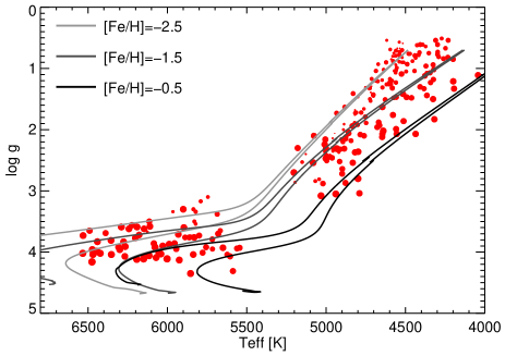
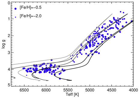
Fig. 2 compares the location of the stars for the parameter sets ${\mathcal{P}}_{\rm LTE,Fe}$ (left panel) and ${\mathcal{P}}_{\rm NLTE,opt}$ (right panel) on the $T_{\mathrm{eff}}$ - $\log g$ plane together with reference stellar evolutionary tracks computed using the GARSTEC code (Weiss & Schlattl, 2008, see next section for a description of the grid of stellar models). Tracks are identical in the left and right plots. Symbol sizes are proportional to [Fe/H] as indicated in the right figure. Even though the tracks are shown only for visual guidance, it is clear that the ${\mathcal{P}}_{\rm NLTE,opt}$ parameters trace the morphology of the turn-off much better. Results for giants are also quite encouraging. For each star with $T_{\mathrm{eff}}<5300$ K, we have searched the entire grid of stellar models the find the best fit to ${\mathcal{P}}_{\rm LTE,Fe}$ and ${\mathcal{P}}_{\rm NLTE,opt}$ parameters as defined by the minimum $\chi^{2}$. In the case of ${\mathcal{P}}_{\rm LTE,Fe}$ parameters, the average minimum $\chi^{2}$ for these stars is 1.9, whereas if ${\mathcal{P}}_{\rm NLTE,opt}$ parameters are used it is 0.4. Clearly, ${\mathcal{P}}_{\rm NLTE,opt}$ parameters lead to an improved overall agreement with stellar tracks.

Figure 2: The location of the stars for the parameter sets ${\mathcal{P}}_{\rm LTE,Fe}$ (left panel) and ${\mathcal{P}}_{\rm NLTE,opt}$ (right panel) on the HRD. For comparison, the reference stellar evolutionary tracks of 0.8 and 1 M_⊙ and metallicities indicated in the legend are overplotted. Symbol sizes are proportional to the metallicity of the observed stars in both panels as indicated in the right plot.

3 Evolutionary tracks

Stellar models have been computed with GARSTEC and detailed information about numerical aspects of the code and the input physics available can be found in Weiss & Schlattl (2008); here we just provide a very brief summary of the most relevant input physics included in the stellar models.

Regarding microphysics, we have used the FreeEOS equation of state (Cassisi et al., 2003) and the ${\rm{}^{14}N(p,\gamma)^{15}O}$ reaction rate recommended by LUNA (Marta et al., 2008). Convection is accounted for by using the standard mixing length theory (Kippenhahn & Weigert, 1990) and the mixing length parameter $\alpha_{\rm MLT}$ is taken from the calibration of a solar model (see below). Convective overshooting is modeled as a diffusive process following the formulation by (Freytag et al. 1996 and see also Eq.3 in Weiss & Schlattl 2008) and the free parameter $f$ is fixed to 0.02. This value represents a moderate amount of overshooting on the main sequence comparable to the canonical 0.2 ${\rm H_{P}}$. However, overshooting has to be limited in small convective cores. In GARSTEC this is now achieved by implementing a geometric cutoff where the extension of the overshooting region decreases quadratically with the ratio between the size of the convective core and the pressure scale height at its boundary (see Magic et al. 2010 for details).

In order to fix the mixing length parameter and the reference composition of our models we have calibrated a standard solar model using the Grevesse & Sauval (1998) solar composition, from which the present-day surface $(Z/X)_{\odot}=0.0229$ and $\log{\epsilon_{\rm Fe}}=7.50$. The latter defines ${\rm[Fe/H]=0}$ in our models. From the calibration we obtain $\alpha_{\rm MLT}=1.811$ and the initial solar helium abundance $Y_{\rm INI}=0.26896$ and metallicity $Z_{\rm INI}=0.01876$. Due to the effects of microscopic diffusion, the initial solar composition corresponds to ${\rm[Fe/H]=+0.06}$.

For the present work, we have computed a dense grid of stellar models in the mass range $0.6\leq M/{\rm M_{\odot}}\leq 1.4$ in steps of 0.01 M_⊙. The initial composition of the models is computed assuming a cosmic helium-to-metal enrichment $\Delta Y/\Delta Z=1.4$ anchored to the initial solar composition. The initial Fe abundance in the grid spans the range ${\rm-5.0\leq[Fe/H]\leq+0.5}$ in steps of 0.1 dex for ${\rm[Fe/H]<0.0}$ and 0.05 dex for ${\rm[Fe/H]>0.0}$ . The set of tracks on which we base the results presented in the following sections include microscopic diffusion and a 0.4 dex $\alpha$-element enhancement for ${\rm[Fe/H]\leq-0.6}$. A maximum depletion of metals due to gravitational settling of about 0.4 dex is obtained for stars typical of the turn-off in metal poor ([Fe/H] $\sim-2$) globular clusters. No additional extra mixing to those mentioned is included in the models. A detailed discussion on this is of no relevance to this work because we are interested in assessing the effect of input spectroscopic parameters in the determination of stellar properties, and these results do not depend on the reference stellar tracks used. Models are evolved from pre-main sequence up to the tip of the RGB or the age $\tau=30$ Gyr, whichever occurs first.

4 Bayesian analysis

Bayesian inference offers a powerful way to characterize a system by allowing the incorporation of prior knowledge into the statistical analysis in an objective way. In the context of our problem, i.e. determination of fundamental stellar parameters, Bayesian methods have been discussed and developed by various authors. Of particular pedagogical interest are the articles by Pont & Eyer (2004) and Jørgensen & Lindegren (2005) and more recent and sophisticated analysis with applications to large stellar surveys can be found in Burnett & Binney (2010), Burnett et al. (2011) and Casagrande et al. (2011). Our implementation of Bayesian inference of basic stellar parameters is described in the next section.

4.1 The Method

In Bayesian analysis, the stellar parameters we want to determine, e.g mass and age, are random variables for which the probability distribution function (PDF) needs to be found. In particular, the posterior PDF, that is the probability of a model being correct given the observed data and the prior knowledge, is expressed as

$$\begin{array}[]{lcl}p(M,\tau,{\rm[Fe/H]}~{}|~{}T_{\rm eff,obs},...)&\propto&p(M,\tau,{\rm[Fe/H]})\\ &&\times\ L(T_{\rm eff,obs},...~{}|~{}M,\tau,{\rm[Fe/H]})\end{array}$$ (1)

where the function $p(M,\tau,{\rm[Fe/H]})$ on the right-hand side represents the prior probability of the stellar parameters and $L(T_{\rm eff,obs},...~{}|~{}M,\tau,{\rm[Fe/H]})$ the likelihood, i.e. the probability of the observed parameters given a model characterized by a set of observables D${}_{j}(M,\tau,{\rm Fe/H]})$. Assuming independence and Gaussian errors in the observed data, the likelihood is

$$L=\prod_{j}\frac{1}{\sqrt{(}2\pi)\sigma_{j}}\ \times\ \exp{\left(-\frac{\left(D_{j}^{\rm obs}-D_{j}^{\rm mod}({\rm M,\tau,[Fe/H]})\right)^{2}}{2\sigma_{j}^{2}}\right)}.$$ (2)

In our case, $D$ consists of three parameters: $T_{\mathrm{eff}}$, $\log g$, and [Fe/H]. Other parameters, like photometric information, can be readily implemented, but we do not consider them here.

The prior probability density of model parameters can be written as

$$p(\tau,M,{\rm[Fe/H]})=p(\tau)\times p({\rm[Fe/H]}~{}|~{}\tau)\times p(M~{}|~{}{\rm[Fe/H]},\tau)$$ (3)

For the prior on mass, we assume a standard Salpeter initial mass function (IMF) independent of age and metallicity. For metallicity we assume a flat prior, i.e. that at all ages all metallicities are a priori equally probable. This simple choice is justified in this work because we are not interested in studying age-metallicity relations for stellar populations and because sufficiently reliable estimates of metallicity are available. Finally, for the age we also assume a flat prior, i.e. that star formation rate (SFR) is constant, but we set a cut at $\tau_{\rm max}=15$ Gyr. Therefore

$$p(M)\sim m^{-2.35},\qquad m\in[0.6,1.4]~{}M_{\odot},$$ (4)

$$p(\tau)\sim 1/\tau_{\rm max},\qquad\tau\in[0,15]~{}{\rm Gyr}.$$ (5)

More complex priors can be elaborated, but our main goal here is to investigate the differences in masses, ages, and distances due to the input spectroscopic parameters rather than to characterize stellar populations.

Finally, the proportionality constant in Eq. 1 is the normalization of the posterior PDF such that $\iiint p(M,\tau,{\rm[Fe/H]}~{}|~{}T_{\rm eff,obs},...)\,{\rm dM\,d\tau\,d[Fe/H]}=1$, and it is of no relevance for the estimation of parameters and uncertainties.

The PDF of a stellar parameter $x$ that takes the values $x_{\rm tr}$ along evolutionary tracks is given by

$$\begin{array}[]{lcl}p(x~{}|~{}T_{\rm eff,obs},...)&=&\iiint\delta\left(x-x_{\rm tr}\right)\\ &&p(M,\tau,{\rm[Fe/H]}\,|\,T_{\rm eff,obs},...)\,dM\,d\tau\,d{\rm[Fe/H]}\end{array}$$ (6)

where the integration is over all evolutionary tracks.

4.2 General properties

A key advantage of Bayesian inference is that, as expressed before, it allows using prior knowledge about the problem being considered. Priors are particularly important when a quantity of interest, affected by the prior, has noticeable changes within the range of observational uncertainties where the likelihood does not change much. A typical example, originally discussed by Pont & Eyer (2004) and further expanded by Jørgensen & Lindegren (2005), is the different evolutionary speed of stellar models that populate the same region of observed parameters. When this is not accounted for, as in methods purely based on maximum likelihood, the results are biased towards faster evolutionary phases, a bias known as the ’terminal-age bias’ (Pont & Eyer, 2004).

To illustrate here the importance of using information not contained in the likelihood, we present a similar example. Let us assume a star has the following observed parameters: $T_{\mathrm{eff}}=6850\pm 50$ K and $\log g=4.05\pm 0.05$ dex. For simplicity, we exclude metallicity in this example by fixing it to [Fe/H] $=-1.0$. In the top panel of Fig. 3 we show three evolutionary tracks of models with different masses overlapping in the range of the observed parameters. While the 1.1 M_⊙ model is entering the subgiant branch (SGB), the 1.2 M_⊙ is on the main sequence (MS) and the 1.3 M_⊙ model is still on the pre-main sequence (PMS).

First, we perform a standard maximum likelihood analysis (hereafter, ML) to determine the stellar mass and age based on Monte-Carlo sampling. We create synthetic distributions of $T_{\mathrm{eff}}$ and $\log g$ assuming Gaussian distributions of errors and search for the best-fit model in all evolutionary tracks of the assumed metallicity. The resulting mass and age distributions are shown in the middle and bottom panels of Fig. 3, respectively. The mass distribution shows a bimodality with a secondary peak and a tail extending towards larger masses ($M>1.2~{}{\rm M_{\odot}}$). The age distribution shows a dominant peak at very low ages (${\rm 6~{}Myr<\tau<10~{}Myr}$) clearly seen in the inset that zooms in in this age range. There are two other local maxima at about 4.3 Gyr and 4.8 Gyr, but with much lower relative probabilities than the solution at very low age. Thus the ML results indicate a strong preference for the PMS solution for the observed parameters.

While it cannot be completely ruled out that the star is on the PMS, considerations of the shortness of this evolutionary phase render this possibility, a priori, not very likely. A ’brute force’ way of taking this into consideration is to directly eliminate PMS models from the analysis. We impose this restriction by removing all stellar models with ages $\tau<20$ Myr. In this way, while the best-fit model is still determined purely from its ML, we are already using prior information by assuming the chance of observing a PMS star is negligible (actually null, although this also is a wrong assumption!). Results for this exercise are labelled ’ML no-PMS’ in the middle and bottom panels of Fig. 3. In the mass distribution, the tail at high masses vanished since its origin was purely from the PMS models. The same is true for the ages: the unrealistically large peak at $\sim 6$ Myr disappeared, and the peaks at 4.3 Gyr and 4.8 Gyr are now the dominant features, but their relative weight is still the same as in the pure ML analysis and the older peak, associated with stars entering the SGB still dominates.

Figure 3: Top panel: degeneracy of evolutionary tracks on the $T_{\mathrm{eff}}-\log g$ plane at the location of our fiducial star (see text). Middle panel: relative probability of the mass distribution functions obtained using pure maximum likelihood (ML - blue dotted line), maximum likelihood with suppressed pre-main sequence models (ML no-PMS - red dashed line), and Bayesian analysis (Bayes - black solid line). Bottom panel: same as above but for the age distribution functions; the inset shows in detail the physically-disfavoured narrow peak corresponding to the pre-main sequence solution (see text for details).

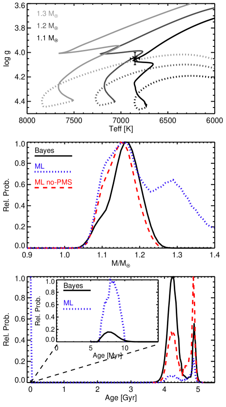
The results of the Bayesian analysis for our fiducial star are also shown in Fig. 3 (middle and bottom panels, solid black line). As in the case of the ML case, three peaks are present but the maximum probability in each of them reflects information not contained in the ML analysis. The PMS solution, although possible, is now strongly disfavoured, whereas the MS solution is now the most likely one and it outweighs the SGB solution. The Bayesian mass distribution (middle panel) is similar to the ML no-PMS case. The vanishing contribution of the PMS is now easy to understand from the eq. 6. The probability for a given mass is obtained by marginalizing the posterior PDF over all possible ages. The stellar tracks with high masses, which contribute in the observational box with the PMS, are strongly disfavoured because of the short duration of this phase. However, the PMS solution still has a non-negligible probability in the age distribution. The widths of the peaks reflect evolutionary speed in each phase, with PMS evolution being about $100$ times faster than late MS evolution and early SGB a few times faster than late MS.

There is one important aspect related to the interpetation of the height of the peaks in the Bayesian age PDF. Strictly speaking, when determining the probability of a given age $p(\tau)$ using Equation 6, there is no information on the speed of stellar evolution because we are looking at a time snapshot. As stated by Jørgensen & Lindegren (2005), the relative heights of the peaks in the age distribution are determined by how closely packed evolutionary tracks of different masses are around the observational error box (i.e., the region over which likelihood is significant and varies little). Where variations in stellar mass introduce small changes on the location of a stellar model (for the same age), the integrand in Equation 6 will vary slowly when integrating in mass. Thus, the interpretation of the height of the peaks as depending on the evolutionary speed of stars is not straightforward. It only follows if slow evolutionary speeds are associated with regions on the observational plane where small changes in mass produce small changes in the observational quantities the determine the likelihood. As stated above, the unique direct manifestation of a slowly evolving phase in the age PDF is the width of the peaks in the distribution.

4.3 Examples

Figure 4: Probability distribution functions (PDFs) for age, mass, and absolute magnitude in the ${\rm K_{S}}$ band. On the left results are shown for a turn-off star and, on the right for a star on the red giant branch. In the latter case, neither mass or age can be determined. The absolute magnitude (luminosity), on the other hand, can be derived precisely in both cases. Black solid lines: Salpeter IMF as a prior in the mass distribution; red dashed lines: flat IFM.

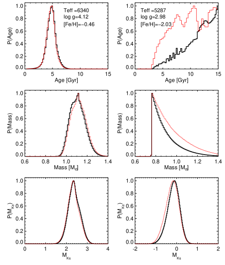
Fig. 4 shows in black thick lines the PDFs of stellar parameters of two stars from our sample. On the left, J112344.9-290327 has [Fe/H] $=-0.46\pm 0.10$, $T_{\mathrm{eff}}=6340\pm 70$ K, and $\log g=4.12\pm 0.10$, i.e. it is a moderately metal-poor turn-off star. In this case, mass, age and absolute $Ks$ magnitude have PDFs that lead to well determined central values and uncertainties. Following Burnett & Binney (2010), we compute stellar parameters and their uncertainty directly from the different moments of the PDFs. In this case, we obtain $\tau=4.78\pm 0.88$ Gyr, ${\rm M=1.108\pm 0.071~{}M_{\odot}}$, and ${\rm M_{Ks}}=2.371\pm 0.279$.

As a second case we have selected J115337.3-020036, with [Fe/H] $=-2.03\pm 0.10$, $T_{\mathrm{eff}}=5287\pm 68$ K, and $\log g=2.98\pm 0.10$, a star on the lower part of the RGB. As it is well known, evolutionary tracks of stars with different masses and similar metallicity are almost degenerate along the RGB in the $T_{\mathrm{eff}}-\log g$ plane (Fig. 2). This degeneracy precludes the determination of its mass and age as seen from the PDFs in Fig. 4. The cut in the age distribution at 15 Gyr simply reflects our age prior, and this corresponds to the mass cut at $\sim 0.75$ M_⊙. The shapes of the PDFs are almost completely determined by the adopted priors, i.e., IMF and SFR, and by the fact that more massive stars evolve faster along the RGB than lower mass stars. No actual information about the true stellar mass and age can be obtained in this case. In fact, a pure likelihood analysis leads to age and mass distributions that are basically flat. On the other hand, the absolute magnitude of this star is still well-defined, and in fact yields ${\rm M_{Ks}}=-0.155\pm 0.289$, the same precision as for the turn-off star. This conclusion remains valid for all stars along the RGB, the absolute magnitude is a well-defined quantity even if the underlying evolutionary tracks are highly degenerate, and we can robustly estimate stellar distances independently of the evolutionary stage of the stars.

Finally, we have tested the impact of the IMF prior by considering also a flat IMF. Results for the two examples just discussed are shown in Figure 4 in red dashed line. Clearly, the impact of changing the IMF is minimal in those cases where stellar parameters are well defined. On the contrary, the large impact of priors in the age and mass distributions for the giant star are evidence that no actual information can be extracted in these cases: the posterior PDF is largely determined by the priors.

5 Results

Using the procedure described in Sect. 4.1 and the two sets, ${\mathcal{P}}_{\rm LTE,Fe}$ and ${\mathcal{P}}_{\rm NLTE,opt}$ of stellar parameters (Section 2), we computed ages, masses and absolute magnitudes for the stars in our sample. To determine the distances, we used the observed 2MASS ${\rm K_{S}}$ magnitudes and the absolute ${\rm K_{S}}$ magnitudes obtained from the Bayesian analysis. The synthetic magnitudes were computed from the MARCS grid of synthetic spectra (Gustafsson et al., 2008) assuming plane-parallel radiative transfer for $\log g>3$ and spherically-symmetric mode otherwise. The synthetic ${\rm K_{S}}$ magnitudes have been computed adopting the absolute calibrations and zero-points discussed in Casagrande et al. (2010). Reddening for each star was computed using Schlegel et al. (1998) maps following the iterative procedure described in Ruchti et al. (2011).

Figure 5: Comparison of ages determined for the sample of nearby stars of Lachaume et al. (1999).

Figure 6: Comparison of distance determination methods. We show distances obtained with our Bayesian scheme and those by the RAVE collaboration (Zwitter et al., 2010). Note that, for this test only, the input stellar parameters ($T_{\mathrm{eff}}$, $\log g$, [Fe/H]) are from the RAVE DR3 catalogue for both distance determinations.

5.1 Tests

In order to assess the robustness of our Bayesian scheme, we selected two sub-samples of stars with basic stellar parameters from Lachaume et al. (1999) and from Zwitter et al. (2010). For the former, we determine ages and compare them with the results from Lachaume et al. (1999). For the latter, we focus on the distances.

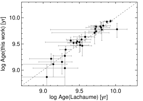
For stellar ages, the comparison only comprises stars for which Lachaume et al. (1999) derived ages from isochrone fitting in order to avoid biases derived from comparing ages obtained with methods not based on stellar evolutionary tracks. The very good agreement (Fig. 5) implies that when the observational uncertainties are small, $1\%$ in $T_{\mathrm{eff}}$ and $0.05$ mag in $M_{v}$, maximum likelihood methods return similar results to the Bayesian analysis and age determinations are robust. A similar agreement was reported by Jørgensen & Lindegren (2005). The uncertainties in the ages we derive are generally smaller compared both to Lachaume et al. (1999) and Jørgensen & Lindegren (2005).

We have derived stellar distances using the input stellar parameters from Zwitter et al. (2010) for the 58 stars common with our sample, and show the results in comparison with RAVE distances (Zwitter et al., 2010) in Fig. 6. Results are an excellent agreement. Therefore, we conclude that, provided the same input stellar parameters are used, our Bayesian scheme and the isochrone matching method by Zwitter et al. (2010) yield very similar results, with no obvious systematic offsets between methods. This is in line with Burnett et al. (2011), who also applied a (more sophisticated) Bayesian analysis to the RAVE stellar sample and found that, although some systematic differences were found, the overall agreement with Zwitter et al. (2010) was good.

5.2 Ages and Masses

Figure 7: Masses and ages for our sample of stars derived with the NLTE-Opt and LTE-Fe basic stellar parameters. Only stars with $\log g>3.6$ are included (see text).

Having verified the reliability of the Bayesian method, we proceed with the analysis of our stellar sample. The degeneracy of stellar tracks discussed in Sec. 4.3 limits the ability to derive masses and ages on the RGB. For this reason, we derived masses and ages for stars with $\log g\geq 3.6$, that is, for $59$ stars only.

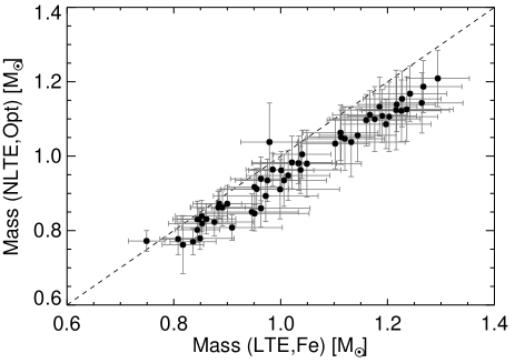
In Fig. 7 we compare masses and ages derived from the two sets ${\mathcal{P}}_{\rm LTE,Fe}$ and ${\mathcal{P}}_{\rm NLTE,opt}$ of input stellar parameters. Stellar masses derived from the ${\mathcal{P}}_{\rm NLTE,opt}$ parameters are systematically lower than those derived from ${\mathcal{P}}_{\rm LTE,Fe}$, by about $0.05-0.1$ M_⊙. The primary reason for the difference lies in the larger gravities obtained with the ${\mathcal{P}}_{\rm NLTE,opt}$ method. Errors of the masses are comparable in both cases, and range between 0.03 M_⊙ up to 0.10 M_⊙. Nevertheless, the systematic shift to lower masses caused by the use of more accurate ${\mathcal{P}}_{\rm NLTE,opt}$ stellar parameters can not be neglected.

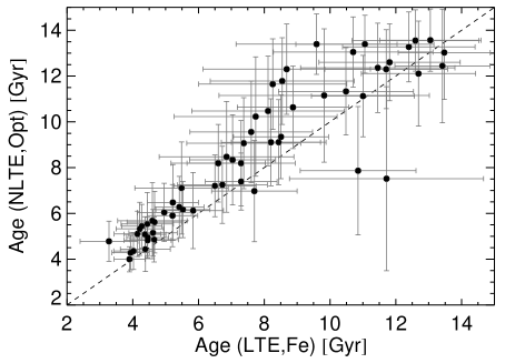
For stellar ages, the behavior is opposite, as expected. The results based on the ${\mathcal{P}}_{\rm NLTE,opt}$ parameters are higher by $10$ to $30$ percent. However, not in all cases a smaller mass implies a larger age. Close inspection of both panels in Fig. 7 reveals only two stars with larger ${\mathcal{P}}_{\rm NLTE,opt}$ masses, whereas six of them have smaller ages derived from ${\mathcal{P}}_{\rm NLTE,opt}$ parameters. Typical uncertainties of our Bayesian ages are of the order of 20% and, except for two cases, range between 10% and 30%. We conclude that the LTE-Fe method underestimates stellar ages by $1-4$ Gyr, and the errors are more pronounced for hotter and more metal-poor stars.

5.3 Distances

The main goal of this section is to show the dramatic impact that using the physically realistic ${\mathcal{P}}_{\rm NLTE,opt}$ stellar parameters has on the determination of stellar distances.

As summarized in Sect. 2, there are large differences between the ${\mathcal{P}}_{\rm LTE,Fe}$ and ${\mathcal{P}}_{\rm NLTE,opt}$ stellar parameters sets. The top panel of Fig. 8 shows the change in the absolute magnitude ${\rm M_{K_{S}}}$ as a function of the $\log g_{\rm NLTE,opt}-\log g_{\rm LTE,Fe}$ differences. The strong linear correlation simply reflects the fact that changes in $\log g$ are accompanied by a reciprocal change in luminosity due to their inverse functional dependence on stellar radius. Clearly, the ${\mathcal{P}}_{\rm NLTE,opt}$ stellar parameters indicate that all our stars, with few exceptions, are fainter than what would be inferred from using the LTE-Fe parameters. Furthermore, if, for the sake of discussion, we neglect the effect of reddening, then distance scales exactly as the square root of the luminosity of the star. Consequently, distances derived from the ${\mathcal{P}}_{\rm LTE,Fe}$ set of parameters are overestimated, as illustrated in Fig. 8 (bottom panel) where we show the ratio of distances derived using ${\mathcal{P}}_{\rm LTE,Fe}$ and ${\mathcal{P}}_{\rm NLTE,opt}$ stellar parameters.

Similar information is provided in Fig. 9 in which the ratio of distances, corrected for reddening, is plotted as a function of $\log g_{\rm LTE,Fe}$. This illustrates clearly how systematic errors in distance determinations impact different stellar types. Stellar metallicities are encoded in the symbol sizes and colours, as indicated in the legend. Distances to metal-rich stars, [Fe/H] $>-1$, are, to first order, unbiased. On the other hand, for metal-poor ([Fe/H] $\leq-1$) dwarfs and sub-giants ($\log g>3.6$), LTE-Fe parameters imply a systematic distance error of about $10-40\%$. The problems are exacerbated at low metallicity and low gravity. Metal-poor giants suffer from the largest fractional distance biases of up to $70\%$.

Figure 8: Changes in the absolute $K_{S}$ magnitudes and distances caused by using the improved set of input basic stellar parameters, ${\mathcal{P}}_{\rm NLTE,opt}$ as a function of the change in $\log g$, for our full sample.

Figure 9: Ratio of distances derived with ${\mathcal{P}}_{\rm LTE,Fe}$ and ${\mathcal{P}}_{\rm NLTE,opt}$ stellar parameters as a function of surface gravity for our full sample. Symbol sizes and colours indicate the stellar metallicity.

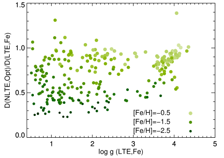
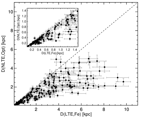
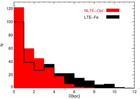
Fig. 12 shows the final distribution of distances determined using the ${\mathcal{P}}_{\rm NLTE,opt}$ and ${\mathcal{P}}_{\rm LTE,Fe}$ stellar parameters for our full sample. This plot summarizes what has already been discussed above, and allows us to put the results into the more general perspective of large-scale stellar surveys. In a magnitude-limited survey, for example, where more metal-rich unevolved stars dominate the nearby sample and metal-poor luminous giants are predominantly observed at large distances, classical full LTE-Fe analysis will systematically overestimate distances, placing stars progressively further than they are. This has important consequences in all cases when stellar metallicities, positions, and kinematics are used for studies of Galactic structure and evolution (Siebert et al., 2008; Carollo et al., 2010; Wilson et al., 2011; Bensby et al., 2011). We touch upon this in Sect. 6.

Figure 10: Comparison of heliocentric distances derived for all stars in our sample using ${\mathcal{P}}_{\rm LTE,Fe}$ and ${\mathcal{P}}_{\rm NLTE,opt}$ sets of basic stellar parameters. In virtually all cases, ${\mathcal{P}}_{\rm LTE,Fe}$ parameters lead to large overestimation of distances.

Figure 11: Differences in basic stellar parameters for the stars in common between our sample and the RAVE distances catalogue (Zwitter et al., 2010). Colours and symbol types are assigned according to $\log g$ values from the DR3 pipeline. Symbol sizes are indicative of the DR3 metallicity, as indicated in the legend. The differences between (NLTE,Opt) and (LTE,Fe) parameters for the same stars are shown in grey empty squares.

Figure 12: Comparison of distances derived using ${\mathcal{P}}_{\rm NLTE,opt}$ stellar parameters and those from the RAVE DR3 catalogue for stars common in both samples. The trend strongly resembles that of the comparison between ${\mathcal{P}}_{\rm LTE,Fe}$ and ${\mathcal{P}}_{\rm NLTE,opt}$ distances (Fig. 12).

5.4 Comparison with other studies: RAVE stellar parameters

Since our sample of stars was drawn from the internal RAVE catalogue, it is very important to investigate how our results, i.e. $T_{\mathrm{eff}}$, $\log g$, [Fe/H], and distances, compare with those obtained by the RAVE collaboration. In what follows, we will compare our data with those by Zwitter et al. (2010), with which we have $58$ stars in common. We highlight the key methodological differences below.

• The quality of observations. Our parameters rely on high-resolution data, R $\sim 30000$, with a very broad wavelength coverage, $3500-9500$ Å; the RAVE spectra have R $\sim 7500$ and cover only a limited wavelength range between $8410$ and $8795$ Å.

• The physics of stellar atmospheres and radiative transfer models. In particular, our analysis relies on NLTE radiative transfer, while the RAVE spectroscopic pipeline operates fully on 1D LTE synthetic spectra.

• The different approaches to determine masses and ages, and stellar evolution models. GARSTEC tracks were used in this work, whereas Zwitter et al. (2010) adopted Padova isochrones. Also, the approach followed in that study is esentially a nearest neighbor technique, however with the important difference that the isochrones were resampled to a uniform spacing in age to account for the variable speed of stellar evolution, and a weighing scheme to include, for example, the impact of the initial mass function. In this respect, their analysis also makes use of priors.

• Zwitter et al. (2010) neglected reddening in their distance determinations. We used the reddening values following Ruchti et al. (2011); also comparison with the interstellar NaD lines in our high-resolution spectra indicates that reddening is not negligible for many stars.

• The uncertainties on our input stellar parameters are typically smaller than those of Zwitter et al. (2010). Their values are $\sim 0.2$ dex in [Fe/H] and $\log g$ and range between $\sim 100$ to 200 K in most cases for $T_{\mathrm{eff}}$, whereas our standard estimates are $60-100$ K in $T_{\mathrm{eff}}$, and $0.1$ dex in [Fe/H] and $\log g$.

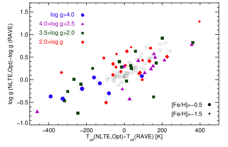
The differences between ${\mathcal{P}}_{\rm NLTE,opt}$ parameters and those from the RAVE DR3 pipeline are shown in Fig. 12. Size and colour of the symbols indicate metallicity and gravity (we used RAVE DR3 values for reference). We also show the differences ${\mathcal{P}}_{\rm NLTE,opt}$ and ${\mathcal{P}}_{\rm LTE,Fe}$ for the same stars in grey empty squares. RAVE DR3 parameters show a very large spread with respect to ${\mathcal{P}}_{\rm NLTE,opt}$. In fact, the spread is much larger than with respect to the ${\mathcal{P}}_{\rm LTE,Fe}$ parameters. Clearly it is not possible to single out specific factors which cause the spread; however, some conclusions can be drawn. In most cases, the RAVE DR3 $\log g$ values are clearly underestimated for giants with $\Delta\log g_{(\rm{NLTE,Opt-RAVE~{}DR3})}$ up to $\sim 1$ dex and one case as large as 1.3 dex. This effect is more pronounced for the metal-poor stars, in qualitative agreement with the differences between the ${\mathcal{P}}_{\rm NLTE,opt}$-${\mathcal{P}}_{\rm LTE,Fe}$ parameters for the same stars. The same is true for subgiants; in most cases the DR3 gravities are underestimated. For dwarfs, on the other hand, we find DR3 gravities are overestimated by as much as 0.5 dex. Burnett et al. (2011) arrive at the same conclusion comparing DR3 gravities with stellar models.

As a consequence of the differences in stellar parameters, particularly changes in $\log g$, the distances we obtain from the ${\mathcal{P}}_{\rm NLTE,opt}$ parameters are systematically smaller than the RAVE DR3 data (Zwitter et al. 2010; Siebert et al. 2011). For the most distant metal-poor giants, the offset is of the order $50$ percent. This is illustrated in Figure 12, which shows that beyond 1.5 kpc all ${\mathcal{P}}_{\rm NLTE,opt}$ distances but one are smaller than those derived in Zwitter et al. (2010). For a few dwarfs in the immediate solar neighborhood, the results are opposite, as expected from the sign of the $\log g$ corrections. The overall trend is very clear and the qualitative similarity with the difference between ${\mathcal{P}}_{\rm NLTE,opt}$ and ${\mathcal{P}}_{\rm LTE,Fe}$ distances (Fig. 12) is striking.

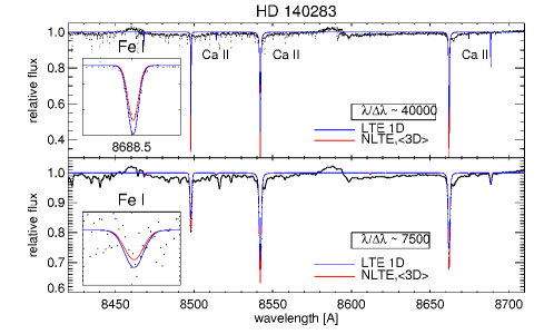
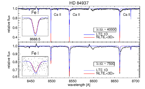
These results provide alarming evidence that the RAVE DR3 stellar parameters are affected by the systematic error caused by the 1D LTE assumption in spectroscopic parameter determinations. Test calculations for the CaII near-IR triplet using the mean 3D model atmospheres from Bergemann et al. (2012) indicate that these spectral lines are strongly affected by the ${\rm 1D-\left<3D\right>}$ differences, while the near-IR Fe I lines are mostly affected by NLTE. Fig. 13 illustrates these effects for the two well-studied metal-poor stars, a subgiant HD 140283 (top plot) and a warm turn-off star HD 84937 (bottom plot) with [Fe/H] $=-2.4$ and $-2$ dex, respectively. The spectra are from Bergemann & Gehren (2008) and shown in the top panels in their original resolution, $R\sim 40\,000$. In the bottom panels the spectra have been degraded to the quality of the RAVE spectra, i.e. $R\sim 7\,500$ and a typical S/N $\sim 50$ (Zwitter et al., 2008, Fig. 8). The $\left<{\rm 3D}\right>$ NLTE synthetic spectra were computed as in Bergemann et al. (2012), but applying LTE radiative transfer to CaII. The 1D LTE radiative transfer models under-estimate the strength of the CaII lines (the effect of $\left<{\rm 3D}\right>$ structure) and over-estimate that of the Fe I lines (the effect of NLTE). Also, the near-IR lines of $\alpha$-elements (Si I, Mg I, and Ti I), which along with Fe I lines dominate the RAVE spectra (Zwitter et al., 2008) all form in NLTE (Zhao & Gehren, 2000; Shi et al., 2011; Bergemann et al., 2012) and it is unlikely that the NLTE effects cancel out to produce a spectrum close to LTE. The effects are clearly present irrespectively of the spectral resolution.

Figure 13: Synthetic 1D LTE (blue) and $<$3D$>$ NLTE (red) spectra of the metal-poor stars HD 140283 (top plot) and HD 84937 (bottom plot). The observed spectra (black points) are from Bergemann & Gehren (2008) in their original resolution, $R\sim 40\,000$ (top panel in each plot), and degraded to the resolution of the RAVE spectra $R\sim 7\,500$ (bottom panel in each plot). The 1D LTE radiative transfer models under-estimate the strength of the Ca II lines and over-estimate that of the Fe I lines (shown in the inset). See text for more details.

We close this section with a few comments related to the two different validations that Zwitter et al. (2010) presented for distance determination from RAVE data. The first one is a comparison with Hipparcos stars present in their catalogue with trigonometric errors smaller than 20% and spectroscopic distance errors smaller than 32%. These results are shown in Figure 3 in Zwitter et al. (2010) and a large spread is present in the comparison. Even if no systematic difference was found, as noted by the authors, almost all these stars dwarfs with a solar-like metallicity ([M/H]=$-0.12\pm 0.25$), exactly the case where we do not expect large NLTE effects. The second test consisted in comparing about 14 stars in 7 open clusters with known distances. Again, all these clusters have solar-like metallicity (Dias et al., 2002) and we do not expect NLTE effects to play a central role. In any case, we note that distances derived by Zwitter et al. (2010, see their Table 2) for the cluster stars deviate from the cluster distances by anything between -20 to +40%. These stars were reanalyzed by Burnett et al. (2011, see their Table 3) and results show a similar spread, although in a few cases distance determinations are also quite different from those in Zwitter et al. (2010). It is simply not possible to try to establish confidence in spectroscopically derived parameters, particularly at low metallicities and gravities, by extrapolating confidence gained by means of tests performed in very different regimes, e.g. at solar metallicity.

6 Summary and conclusions

This paper is the second in the series where we explore the influence of different methods on the determination of basic and fundamental stellar parameters for FGKM stars. The main goal is to understand to what extent our knowledge about stars, their surface and interior structure, is biased by inferences derived from classical model atmospheres with their simplifying assumptions (1D hydrostatic and local thermodynamic equilibrium, LTE), which have been used as a basis for spectroscopic characterization of stars over the past $70$ years.

Figure 14: Heliocentric spatial distribution of stars in our sample. Top and bottom panels respectively show results obtained based on ${\mathcal{P}}_{\rm LTE,Fe}$ and ${\mathcal{P}}_{\rm NLTE,opt}$ parameters. Colours depict the stellar surface gravity as indicated in the plots.

In Paper 1, we developed a novel NLTE-Opt technique to determine accurate effective temperature, surface gravity, and metallicity from a stellar spectrum and then applied the method to a large sample of stars selected from the RAVE survey. The principal components of the method are (i) the use of a robust effective temperature scale from the analysis of Balmer line wings and, (ii) the determination of surface gravities and metallicities by solving physically-realistic NLTE radiative transfer in Fe lines. This avoids substantial systematic uncertainties in parameters introduced by the commonly-used approximation of LTE. A comparison of the new NLTE-Opt stellar parameters to that obtained from the standard method of 1D LTE excitation-ionization balance of Fe, LTE-Fe, revealed important differences ranging from $-100$ K to $+400$ (subgiants, RGB) in $T_{\rm eff}$, $0.1$ to $1.5$ dex in $\log g$, and $0.05$ to $0.5$ dex in [Fe/H].

In this paper, we focus on the determination of evolutionary parameters of stars, masses and ages, and their distances. We develop a robust Bayesian technique using state-of-the-art evolutionary tracks computed with the GARSTEC code (Weiss & Schlattl, 2008). The importance of the Bayesian scheme in this context has been raised in several earlier studies (Pont & Eyer, 2004; Jørgensen & Lindegren, 2005). This method has a principal advantage over standard maximum likelihood (or minimum $\chi^{2}$) methods in that it allows a simple way of introducing additional (prior) knowledge in the statistical analysis. Test comparisons of results obtained with our Bayesian scheme with other similar studies confirm its reliability and accuracy.

We then apply the Bayesian method to both sets of stellar parameters, LTE-Fe and NLTE-Opt, for the sample of stars from our Paper 1. The stars were selected from the RAVE catalogue. They cover the full parameter space in $T_{\rm eff}$ ($3500$ to $6500$ K), $\log g$ ($3500$ to $6500$), and [Fe/H] ($-3.0$ to $-0.5$) and sample the local volume within $\sim 10$ kpc. Spectroscopic distances were computed for all these stars using the 2MASS photometry. Masses and ages were determined for the $59$ dwarf and subgiant stars ($\log g>3.6$) only, the limit set by the degeneracy of stellar tracks of different mass along the RGB in the $T_{\mathrm{eff}}-\log g$ plane.

From these calculations, the following conclusions can be drawn.

• The classical method of LTE excitation-ionization balance of Fe, as a rule, underestimates ${\rm Teff}$, $\log g$, and [Fe/H] of FGKM stars. As demonstrated in Paper 1, for the most metal-poor giants, [Fe/H] $\sim-3$, the errors are of the order $+0.5$ dex in metallicity. This has implications for the metallicity distribution function of stars in different Galactic components. For our stellar sample, which is representative of the thick-disk, the metal-poor end of the MDF steepens and is skewed towards the more metal-rich domain (by $\Delta$[Fe/H] $\sim+0.3$ dex; Bergemann et al., 2013).

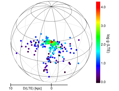
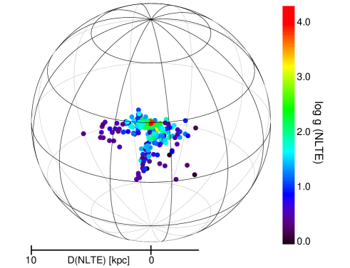
• LTE-Fe stellar parameters result in overestimated distances compared to the NLTE-Opt results, and the bias depends on the metallicity and evolutionary stage of a star. The changes in surface gravity are most critical for metal-poor RGB stars, for which the NLTE-Opt distances are smaller by up to $70\%$. The distances to metal-poor subgiant and turnoff stars are in error by a factor of $2$. Only more metal-rich turn-off stars are barely affected by this bias. Fig. 14 shows the spatial heliocentric distribution of the stars in our sample determined with ${\mathcal{P}}_{\rm LTE,Fe}$ (top panel) and ${\mathcal{P}}_{\rm NLTE,opt}$ (bottom panel) parameters and makes evident the large impact of using inaccurate stellar parameters for deriving spectrophotometric distances, in particular for giants with $\log g<2.0$. The overall distribution of distances in our sample steepens towards smaller distances as shown in Fig. 15. As a consequence, significant errors may enter the determination of space velocities and orbital eccentricities, and differences in the population membership of stars (i.e. thick disk or halo) are expected.

• Comparing our NLTE-Opt results with the RAVE DR3 distances (Zwitter et al., 2010) for the stars common in both samples we find a pattern similar to the comparison between NLTE-Opt and LTE-Fe results. This is not surprising: metal lines that dominate the near-IR RAVE spectra are known to be strongly affected by NLTE effects (Sect. 5.4) and our test calculations with mean 3D models also show that the lines are sensitive to the ${\rm 1D-\left<3D\right>}$ atmospheric structure differences. As a result, more distant stars (predominantly metal-poor giants) have larger DR3 distances compared to our values (Fig. 12), by $10-50\%$.

  In this respect, it is very interesting to interpret our results in the light of the findings by Schönrich et al. (2011) where the authors concluded, based on simple analytical considerations that distances for SDSS/SEGUE metal-poor stars are systematically overestimated. Consistent with the arguments presented in that study, our calculations predict that the systematic error in $\log g$ and, thus, distance increases with decreasing metallicity; [Fe/H] is affected too, although at a lesser degree. Thus, there will be two effects. First, more metal-poor stars will appear more luminous and thus more distant, which may be mis-interpreted for a very metal-poor outer stellar population. This goes in the direction of explaining why this component would appear to be more metal poor than the inner halo component. Second, the systematic error in distance may propagate into the error in transverse velocity, causing the effect of a star on a retrograde orbit. This strengthens the claim by Schönrich et al. (2011) that the available observational evidence for a counter-rotating Galactic halo component (Carollo et al., 2010) is weak.

• Masses and ages are likewise affected in a systematic way by the differences between NLTE-Opt and LTE-Fe, although there is not a one-to-one mapping of the change in mass to the change in age. In the LTE-Fe method, the majority of stars appear younger and slightly more massive. The difference with NLTE-Opt is of the order $0.05-0.1$ M_sun. The ages are inaccurate by anything between $10$ and $30$ percent. In this respect, it will be interesting to re-investigate the age-metallicity relation in the solar neighborhood, which is usually drawn from stellar samples with spectroscopic metallicities and ages obtained by simple isochrone fitting.

Figure 15: Distribution of distances for our full sample showing the global impact of using the physically realistic ${\mathcal{P}}_{\rm NLTE,opt}$ stellar parameters to estimate distances.

We emphasize that, contrary to a wide-spread impression, departures from LTE and 1D hydrostatic equilibrium will affect low- and high-resolution spectra. The reason is that these effects change equivalent widths (or, equivalently, line indices), and consequently abundances inferred from a diagnostic feature. This can not be compensated by decreasing resolution of a spectrum, which merely alters the line profile shape without affecting the total energy absorbed in a line.

In summary, we have shown that the accuracy of the stellar parameters ($T_{\mathrm{eff}}$, $\log g$ and [Fe/H]) is crucial to obtain reliable masses, ages, and spectroscopic distances for late-type stars. Our findings lead to the inevitable conclusion that using the adequate $T_{\mathrm{eff}}$ scale and accounting for the deviations from LTE and 1D hydrostatic equilibrium in stellar atmospheres is of fundamental importance if we want to achieve an accurate characterization of stellar populations. Until now, most of the work in the community has gone into developing sophisticated statistical methods to extract the largest possible amount of information from large-scale stellar surveys. Although these efforts are undoubtedly valuable, they will not cure the major problem affecting the final distributions of masses, ages, metallicities, distances, which arises because systematic errors in basic stellar parameters dominate. We thus advise particular caution when applying stellar parameters obtained from 1D LTE models in studies of stellar populations.

References

- Asplund (2005) Asplund M., 2005, ARAA, 43, 481
- Bensby et al. (2011) Bensby T., Alves-Brito A., Oey M. S., Yong D., Meléndez J., 2011, ApJL, 735, L46
- Bergemann & Gehren (2008) Bergemann M., Gehren T., 2008, A&A, 492, 823
- Bergemann et al. (2012) Bergemann M., Kudritzki R.-P., Plez B., Davies B., Lind K., Gazak Z., 2012, ApJ, 751, 156
- Bergemann et al. (2012) Bergemann M., Lind K., Collet R., Magic Z., Asplund M., 2012, ArXiv e-prints
- Bergemann et al. (2013) Bergemann M., Serenelli A., Ruchti G., 2013, Proceedings of the IAU 289, Cambridge University Press
- Breddels et al. (2010) Breddels M. A., Smith M. C., Helmi A., Bienaymé O., Binney J., Bland-Hawthorn J., Boeche C., Burnett B. C. M., Campbell R., et al. 2010, A&A, 511, A90
- Burnett & Binney (2010) Burnett B., Binney J., 2010, MNRAS, 407, 339
- Burnett et al. (2011) Burnett B., Binney J., Sharma S., Williams M., Zwitter T., Bienaymé O., Bland-Hawthorn J., Freeman K. C., Fulbright J., et al. 2011, A&A, 532, A113
- Carollo et al. (2010) Carollo D., Beers T. C., Chiba M., Norris J. E., Freeman K. C., Lee Y. S., Ivezić Ž., Rockosi C. M., Yanny B., 2010, ApJ, 712, 692
- Casagrande et al. (2010) Casagrande L., Ramírez I., Meléndez J., Bessell M., Asplund M., 2010, A&A, 512, A54+
- Casagrande et al. (2011) Casagrande L., Schönrich R., Asplund M., Cassisi S., Ramírez I., Meléndez J., Bensby T., Feltzing S., 2011, A&A, 530, A138
- Cassisi et al. (2003) Cassisi S., Salaris M., Irwin A. W., 2003, ApJ, 588, 862
- Dias et al. (2002) Dias W. S., Alessi B. S., Moitinho A., Lépine J. R. D., 2002, A&A, 389, 871
- Freytag et al. (1996) Freytag B., Ludwig H.-G., Steffen M., 1996, A&A, 313, 497
- Gai et al. (2011) Gai N., Basu S., Chaplin W. J., Elsworth Y., 2011, ApJ, 730, 63
- Gilmore et al. (2012) Gilmore G., Randich S., Asplund M., Binney J., Bonifacio P., Drew J., Feltzing S., Ferguson A., Jeffries R., et al 2012, The Messenger, 147, 25
- Grevesse & Sauval (1998) Grevesse N., Sauval A. J., 1998, Space Sci. Rev., 85, 161
- Gustafsson et al. (2008) Gustafsson B., Edvardsson B., Eriksson K., Jørgensen U. G., Nordlund Å., Plez B., 2008, A&A, 486, 951
- Holmberg et al. (2007) Holmberg J., Nordström B., Andersen J., 2007, A&A, 475, 519
- Jørgensen & Lindegren (2005) Jørgensen B. R., Lindegren L., 2005, A&A, 436, 127
- Kippenhahn & Weigert (1990) Kippenhahn R., Weigert A., 1990, Stellar Structure and Evolution. Springer-Verlag Berlin Heidelberg New York
- Lachaume et al. (1999) Lachaume R., Dominik C., Lanz T., Habing H. J., 1999, A&A, 348, 897
- Lee et al. (2008) Lee Y. S., Beers T. C., Sivarani T., Allende Prieto C., Koesterke L., Wilhelm R., Re Fiorentin P., Bailer-Jones C. A. L., Norris J. E., Rockosi C. M., Yanny B., Newberg H. J., Covey K. R., Zhang H.-T., Luo A.-L., 2008, AJ, 136, 2022
- Lind et al. (2012) Lind K., Bergemann M., Asplund M., 2012, ArXiv e-prints
- Liu & Chaboyer (2000) Liu W. M., Chaboyer B., 2000, ApJ, 544, 818
- Magic et al. (2010) Magic Z., Serenelli A., Weiss A., Chaboyer B., 2010, ApJ, 718, 1378
- Marta et al. (2008) Marta M., Formicola A., Gyürky G., Bemmerer D., Broggini C., Caciolli A., Corvisiero P., Costantini H., Elekes Z., et al. 2008, Phys. Rev. C, 78, 022802
- Mashonkina et al. (2007) Mashonkina L., Korn A. J., Przybilla N., 2007, A&A, 461, 261
- Munari et al. (2005) Munari U., Sordo R., Castelli F., Zwitter T., 2005, A&A, 442, 1127
- Ng & Bertelli (1998) Ng Y. K., Bertelli G., 1998, A&A, 329, 943
- Nordström et al. (2004) Nordström B., Mayor M., Andersen J., Holmberg J., Pont F., Jørgensen B. R., Olsen E. H., Udry S., Mowlavi N., 2004, A&A, 418, 989
- Pont & Eyer (2004) Pont F., Eyer L., 2004, MNRAS, 351, 487
- Ruchti et al. (2012) Ruchti G., Bergemann M., Serenelli A., Casagrande L., Lind K., 2012, MNRAS, doi: 10.1093/mnras/sts319, Paper 1
- Ruchti et al. (2011) Ruchti G. R., Fulbright J. P., Wyse R. F. G., Gilmore G. F., the RAVE collaboration 2011, ApJ, 737, 9
- Schlegel et al. (1998) Schlegel D. J., Finkbeiner D. P., Davis M., 1998, ApJ, 500, 525
- Schönrich et al. (2011) Schönrich R., Asplund M., Casagrande L., 2011, MNRAS, 415, 3807
- Shi et al. (2011) Shi J. R., Gehren T., Zhao G., 2011, A&A, 534, A103
- Siebert et al. (2008) Siebert A., Bienaymé O., Binney J., Bland-Hawthorn J., Campbell R., the RAVE collaboration 2008, MNRAS, 391, 793
- Siebert et al. (2011) Siebert A., Williams M. E. K., Siviero A., Reid W., Boeche C., Steinmetz M., Fulbright J., Munari U., Zwitter T., et al. 2011, AJ, 141, 187
- Steinmetz et al. (2006) Steinmetz M., Zwitter T., Siebert A., Watson F. G., Freeman K. C., Munari U., Campbell R., Williams M., Seabroke G. M., et al. 2006, AJ, 132, 1645
- Takeda et al. (2007) Takeda G., Ford E. B., Sills A., Rasio F. A., Fischer D. A., Valenti J. A., 2007, ApJS, 168, 297
- Valenti & Fischer (2005) Valenti J. A., Fischer D. A., 2005, ApJS, 159, 141
- Weiss & Schlattl (2008) Weiss A., Schlattl H., 2008, Astrophysics and Space Science, 316, 99
- Wilson et al. (2011) Wilson M. L., Helmi A., Morrison H. L., Breddels M. A., the RAVE collaboration 2011, MNRAS, 413, 2235
- Yanny et al. (2009) Yanny B., Rockosi C., Newberg H. J., Knapp G. R., Adelman-McCarthy J. K., Alcorn B., Allam S., Allende Prieto C., An D., et al. 2009, AJ, 137, 4377
- Zhao & Gehren (2000) Zhao G., Gehren T., 2000, A&A, 362, 1077
- Zwitter et al. (2010) Zwitter T., Matijevic G., Breddels M. A., Smith M. C., the RAVE collaboration 2010, A&A, 522, A54
- Zwitter et al. (2008) Zwitter T., Siebert A., Munari U., Freeman K. C., the RAVE collaboration 2008, AJ, 136, 421