Low Mach Number Modeling of Convection in Helium Shells on Sub-Chandrasekhar White Dwarfs. I. Methodology

Abstract

We assess the robustness of a low Mach number hydrodynamics algorithm for modeling helium shell convection on the surface of a white dwarf in the context of the sub-Chandrasekhar model for Type Ia supernovae. We use the low Mach number stellar hydrodynamics code, MAESTRO, to perform three-dimensional, spatially-adaptive simulations of convection leading up to the point of the ignition of a burning front. We show that the low Mach number hydrodynamics model provides a robust description of the system.

1 Introduction

Sub-Chandrasekhar models for Type Ia form an attractive progenitor candidate because of the abundance of low mass white dwarfs. The modern model of these explosions traces back to the work of Livne (1990); Livne & Glasner (1990); Woosley & Weaver (1994); Wiggins & Falle (1997); Wiggins et al. (1998) amongst others. In this “double detonation” model, a detonation ignited in the accreted helium layer on the surface of a low mass carbon/oxygen white dwarf drives a shock inward, compressing the star and initiating a detonation in the core. At the time of these calculations, a common concern was that the lack of resolution in simulations prevented a realistic investigation of these events. Recently, however, the sub-Chandrasekhar mass progenitor model of Type Ia supernovae has seen renewed interest (Fink et al., 2007, 2010; Sim et al., 2010; Shen et al., 2010), as observations show an increasing diversity of SNe Ia events.

As in the traditional Chandrasekhar-mass model of SNe Ia, the ignition of a burning front is preceded by a long period of convection. Here, however, the convection takes place in the He layer, driven by reactions at the base of the layer. To date, numerical simulations of this type of explosion have been initialized by seeding a detonation in the He layer. However, it remains an open question as to whether the turbulent convective flow in the He layer can ignite a detonation in the first place; it is also quite possible that there can be multiple nearly-simultaneous ignitions (see for example, García-Senz et al. 1999).

A potential issue with this model is that a detonation in the He shell would produce large amounts of ⁵⁶Ni at the edge of the star that is inconsistent with observations (Hoeflich & Khokhlov, 1996; Hoeflich et al., 1996) (also see Nugent et al. 1997 for additional concerns about the spectra). The mass of the He layer is uncertain, and it has been suggested that one way to address the overproduction of Ni is for the He shell to be very thin, in which case it may be able to detonate without over-producing surface ⁵⁶Ni (Fink et al., 2010; Kromer et al., 2010). Detailed one-dimensional stellar evolution calculations suggest that the helium in these smallest mass shells may never ignite as a detonation to begin with (Woosley & Kasen, 2011). If it does ignite, Townsley et al. (2012) showed that a robust detonation can propagate through the layer.

The dynamics of the convection and development of a burning front in the sub-Chandrasekhar model is inherently multidimensional. Because the fluid and flame velocities in this initial phase are much lower than the sound speed, we can apply the same low Mach number methodology used to study ignition in the Chandrasekhar-mass scenario (Zingale et al., 2009, 2011; Nonaka et al., 2012). Once we ensure that we have a robust simulation methodology, there is a large parameter space of initial models to explore. The goal of this first paper is to demonstrate that low Mach number hydrodynamics provides an efficient and accurate simulation platform to explore the convective stage of these sub-Chandra events.

2 Numerical Methodology

To study the turbulent convection in the sub-Chandrasekhar model, we use the MAESTRO code as documented in Nonaka et al. (2010). For an overview of the low Mach number equations and numerical methodology, we refer the reader to Section 2.1 of Nonaka et al. (2012). In summary, MAESTRO is a finite-volume, adaptive mesh stellar hydrodynamics code that models the flow using a low Mach number approximation—sound waves are filtered out of the system, but compressibility effects due to stratification and local heat release are retained. For most of the simulations presented here, the star is modeled on a Cartesian grid with the center of the white dwarf at the coordinate origin, i.e., we model one octant of the full star. Since the convection is confined to the outer shell, away from the center of the star, this geometry captures the convective behavior well. The base state pressure and density are represented by one-dimensional radial profiles which capture the hydrostatic state of the star. As in the simulations in Zingale et al. (2009, 2011); Nonaka et al. (2012), we derive the temperature from the equation of state given the pressure, density and mass fractions, rather than evolving the enthalpy equation. Below we provide additional details specific to the simulations presented here; these introduce a variety of parameters that will be explored in the results section.

2.1 Microphysics

We use a general, publicly available equation of state consisting of ions, radiation, and arbitrarily degenerate/relativistic electrons, together with Coulomb corrections (Timmes, 2008; Timmes & Swesty, 2000). We use a simple reaction network consisting of the triple-alpha and ${}^{12}\mathrm{C}(\alpha,\gamma)^{16}\mathrm{O}$ reactions. The rates are from Caughlan & Fowler (1988), with screening as in Graboske et al. (1973); Weaver et al. (1978); Alastuey & Jancovici (1978); Itoh et al. (1979). The ${}^{12}\mathrm{C}(\alpha,\gamma)^{16}\mathrm{O}$ reaction rate has been multiplied by 1.7 as suggested by Weaver & Woosley (1993) and Garnett (1997). This network is an extension of the network used by Malone et al. (2011). When computing the effect of reactions over a time interval, we evolve the temperature along with the mass fractions, keeping the thermodynamic derivatives frozen during the integration, as described in Almgren et al. (2008).

2.2 Initial Model

For simplicity, we construct our own one-dimensional, semi-analytic initial model of a white dwarf with a helium layer. This allows us to control specific features as we learn about the algorithmic sensitivity to the choice of initial model parameters. The initial model is constructed with an isothermal C white dwarf with an isentropic He layer on the surface. When initializing the data on the three-dimensional grid, we interpolate from this initial model and then apply a velocity perturbation, the latter described in Section 2.5.

To construct the initial model, we use the following iterative process:

• We start by providing an estimate for the white dwarf central density, $\rho_{\mathrm{core}}$, and the density at which we transition to helium, $\rho_{\mathrm{He}}$. We also specify the composition of the core, $X_{\mathrm{core}}$, and its temperature, $T_{\mathrm{core}}$, and compute the central pressure via the equation of state, $p_{\mathrm{core}}=p(\rho_{\mathrm{core}},T_{\mathrm{core}},X_{\mathrm{core}})$.

• We then construct our model by integrating outward from the center and iterate over the central density and transition density until the mass of the core, $M_{\mathrm{WD}}$ and the mass of the helium envelope, $M_{\mathrm{He}}$, are the desired values.

  To be more precise, given $\rho_{\mathrm{core}}$ and $\rho_{\mathrm{He}}$, we do the following:

  • Specify the composition for zone $i$:

    $$X_{i}=\left\{\begin{array}[]{ll}X_{\mathrm{core}}&\mathrm{if~{}}\rho_{i-1}>\rho_{\mathrm{He}}\\ X_{\mathrm{core}}+\frac{1}{2}(X_{\mathrm{He}}-X_{\mathrm{core}})\left[1+\tanh\left(\frac{x_{i}-x_{\mathrm{He}}-4\delta}{\delta}\right)\right]&\mathrm{if~{}}\frac{1}{2}\left[1+\tanh\left(\frac{x_{i}-x_{\mathrm{He}}-4\delta}{\delta}\right)\right]<0.999\\ X_{\mathrm{He}}&\mathrm{otherwise}\end{array}\right.$$ (1)

    here, $\delta$ is the width of the transition layer and $x_{\mathrm{He}}=x(\rho_{\mathrm{He}})$ is the coordinate corresponding to $\rho_{\mathrm{He}}$. It is important that $\delta$ be resolved on our grid.

  • Specify the temperature

    $$T_{i}=\left\{\begin{array}[]{ll}T_{\mathrm{core}}&\mathrm{if~{}}\rho_{i-1}>\rho_{\mathrm{He}}\\ T_{\mathrm{core}}+\frac{1}{2}(T_{\mathrm{base}}-T_{\mathrm{core}})\left[1+\tanh\left(\frac{x_{i}-x_{\mathrm{He}}-4\delta}{\delta}\right)\right]&\mathrm{if~{}}\frac{1}{2}\left[1+\tanh\left(\frac{x_{i}-x_{\mathrm{He}}-4\delta}{\delta}\right)\right]<0.999\\ \max\{T(s_{\mathrm{He}},\rho_{i},X_{i}),T_{\mathrm{cutoff}}\}&\mathrm{otherwise}\end{array}\right.$$ (2)

    here, $T_{\mathrm{base}}$ is the desired temperature at the base of the He layer, and $s_{\mathrm{He}}$ is the specific entropy of the base, $s_{\mathrm{He}}=s(\rho_{\mathrm{base}},T_{\mathrm{base}},X_{\mathrm{base}})$. Finally, $T_{\mathrm{cutoff}}$ is the lowest temperature allowed in the outer envelope.

    In both of these profiles, a tanh profile was used at the base of the layer. The true functional form of the transition is not known. Adopting a tanh gives it a smoothness that is desirable for hydrodynamics codes while still keeping the transition narrow.

  • Compute the pressure using the equation of hydrostatic equilibrium (HSE). We difference the HSE equation as:

    $$p^{\mathrm{HSE}}_{i}=p_{i-1}+\frac{1}{2}\Delta r(\rho_{i}+\rho_{i-1})g_{i-1/2}$$ (3)

    Here $g_{i-1/2}$ is the gravitational acceleration at the lower edge of the zone, computed as $g_{i-1/2}=-GM_{\mathrm{encl}}/x_{i-1/2}^{2}$, where $M_{\mathrm{encl}}$ is the mass integrated up to that edge. Given our guess for the density in the zone, $\rho_{i}$, the equation of state will return a pressure $p^{\mathrm{EOS}}_{i}=p(\rho_{i},T_{i},X_{i})$. We define a function, $F$, as $F=p^{\mathrm{HSE}}_{i}-p^{\mathrm{EOS}}_{i}$ and use a Newton-Raphson iteration to find the $\rho_{i}$ needed to zero $F$. In the case where we are constraining the profile to be isentropic (with constant entropy $s_{\mathrm{He}}$) we begin with a guess for $T_{i}$, and zero an additional function, $G=s_{\mathrm{He}}-s^{\mathrm{EOS}}_{i}$, where $s^{\mathrm{EOS}}_{i}=s(\rho_{i},T_{i},X_{i})$. In this case, zeroing both $F$ and $G$ yield $\rho_{i}$ and $T_{i}$.

  • After all zones are computed, compute $M_{\mathrm{WD}}$ by integrating up all the carbon (and oxygen if present), and $M_{\mathrm{He}}$ by integrating up all the helium. We then correct $\rho_{\mathrm{core}}$ and $\rho_{\mathrm{He}}$ using a secant method, recompute $p_{\mathrm{core}}$, and iterate the above procedure until the model is converged.

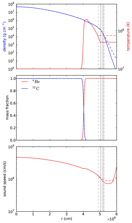
For the current simulations, we use two slightly different models. For both, we set $X_{\mathrm{core}}$ to be pure carbon and $X_{\mathrm{He}}$ to be pure helium. (The reason we leave oxygen out of the white dwarf for these initial models is to allow us to easily use the oxygen generated by the reactions as a tracer of the nucleosynthesis). We pick $M_{\mathrm{WD}}=1~{}\mathrm{M}_{\odot}$ (here, $M_{\mathrm{WD}}$ is the integrated mass of the carbon only), $M_{\mathrm{He}}=0.05~{}\mathrm{M}_{\odot}$, $T_{\mathrm{core}}=10^{7}~{}\mathrm{K}$, $T_{\mathrm{base}}=2\times 10^{8}~{}\mathrm{K}$, and $\delta=5\times 10^{6}~{}\mathrm{cm}$. This value of $\delta$ ensures that the composition gradients are somewhat smoothed. The only difference between the models is the choice of cutoff temperature above the convective zone. Our cool model has $T_{\mathrm{cutoff}}=5\times 10^{7}~{}\mathrm{K}$, and our hotter model has $T_{\mathrm{cutoff}}=7.5\times 10^{7}~{}\mathrm{K}$. Figure 1 shows the profile for both models. The cool model is indicated by the solid lines and the hot model is the dashed lines. When creating these models, we pick a zone width, $\Delta r$, to be $1/5^{\mathrm{th}}$ of the Cartesian zone width, $\Delta x$.

It is interesting to look at the behavior of the sound speed in the initial model, shown in the lower panel of Figure 1. For very low Mach number flows, the time step for a compressible algorithm (assuming uniform zoning) will be set where the sound speed is highest—the center of the star. For the low Mach number algorithm, it will be set where the velocities are the highest—presumably in the convectively unstable region. But the highest Mach number in our simulations is not necessarily there as well—it is likely to be at the very edge of the star, where the velocity will rise due to the density gradient, but the sound speed is small relative to the sound speed at the core. For this reason, we may realize a moderately large Mach number just outside the star ($\sim 0.2$–$0.3$), but still be able to take a time step an order-of-magnitude larger than a compressible code, because the peak Mach number is not where the sound speed peaks. We note that the upturn in sound speed at the largest radii shown in Figure 1 is not mapped into our computational domain because of the use of a low density cutoff. This upturn arises because of the dominance of the radiation pressure in the general equation of state, a behavior that is unphysical outside the star.

2.3 Simulation Parameters

We use the same set of cutoff densities and sponging techniques described in Zingale et al. (2011); Nonaka et al. (2012). These parameters are designed to eliminate large velocities that arise due to the steep density gradient at the edge of the star, outside of our region of interest.

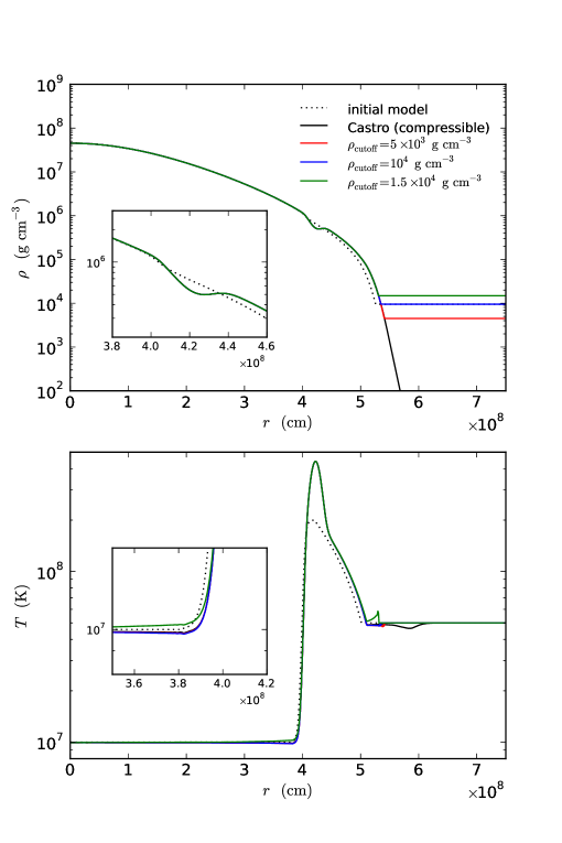
A low density cutoff, $\rho_{\mathrm{cutoff}}$, is the minimum density used in the initial model—outside of that radius in the star, $r_{\mathrm{cutoff}}=r(\rho_{\mathrm{cutoff}})$, we hold the density constant. The material at $r>r_{\mathrm{cutoff}}$ does not contribute to the computation of the gravitational acceleration. To determine a reasonable value of $\rho_{\mathrm{cutoff}}$, we perform a one-dimensional base state expansion test, comparing the results to the compressible code CASTRO (Almgren et al., 2010b). Figure 2 shows the results of placing our initial model onto a one-dimensional spherical grid and heating it for 25 s with a heating term:

$$H=A_{\mathrm{heat}}X(^{4}\mathrm{He})e^{-(r-r_{\mathrm{heat}})^{2}/\sigma_{\mathrm{heat}}^{2}}$$ (4)

We choose $A_{\mathrm{heat}}=10^{15}~{}\mathrm{erg~{}g^{-1}~{}s^{-1}}$, $r_{\mathrm{heat}}=4.2\times 10^{8}~{}\mathrm{cm}$, and $\sigma_{\mathrm{heat}}=10^{7}~{}\mathrm{cm}$. These values were chosen to concentrate the energy release at the base of the He layer and to ensure that we see a significant response to the hydrostatic structure. The base state expansion algorithm used in MAESTRO is described in detail in Nonaka et al. (2010). We run with three different choices of $\rho_{\mathrm{cutoff}}$: $5\times 10^{3}$, $10^{4}$, and $1.5\times 10^{4}$ g cm^-3. The figure shows excellent agreement between the fully compressible (CASTRO) results and MAESTRO’s base state expansion. We note that this is a rather severe test, and the amount of expansion seen here is greater than what we expect in our three-dimensional simulations. There is a slight departure from the compressible solution at the base of the helium layer in the temperature field for the largest choice of $\rho_{\mathrm{cutoff}}$. Based on these results, we choose $\rho_{\mathrm{cutoff}}=10^{4}~{}\mathrm{g~{}cm^{-3}}$ for the simulations presented here. As in Zingale et al. (2011); Nonaka et al. (2012) we have a cutoff to the buoyancy term in the momentum equation which we set as $2\rho_{\mathrm{cutoff}}$. It is important to note that this one-dimensional test does not have any transport of the energy, it simply expands the hydrostatic structure in response to the heating. As a result, the large increase in temperature seen here will not appear in the actual three-dimensional simulation (since convection would redistribute the heat).

Outside of the star, we want to damp away large velocities, as this region is not really part of the simulation space and we do not want velocities here to build up and influence our time step. In MAESTRO, this is accomplished through the use of a sponge, which appears as a source in the velocity equation. The sponge has the same functional form as presented in Zingale et al. (2009) and as refined in Zingale et al. (2011); Nonaka et al. (2012). In particular, we define a density at which to center the sponge, $\rho_{\mathrm{md}}$, and a multiplicative factor, $f_{\mathrm{sp}}$, to mark the start of the sponge. This means that the sponging turns on (gradually) once the model drops below a density of $f_{\mathrm{sp}}\rho_{\mathrm{md}}$. We chose the sponge parameters to make the sponge turn on at the top of the convective layer. Finally, we modify the constraint equation to act like the anelastic constraint to suppress high velocities at the outer boundary of the star (see Almgren et al. 2008). This occurs once the density drops below $\rho_{\mathrm{anelastic}}$. Table 1 summarizes the cutoff parameters for the two different initial models. These parameters are illustrated in Figure 1 as the vertical lines, again with the solid corresponding to the cooler cutoff model and the dashed to the hotter cutoff model.

2.4 Grid Structure

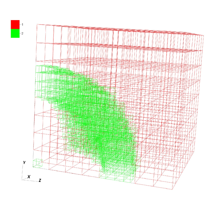
Adaptive mesh refinement is used, with the refinement tagging on zones that have $X(^{4}\mathrm{He})>0.01$ and $\rho\geq\rho_{\mathrm{cutoff}}$. Additionally, we always refine the very center of the star (the coordinate origin) due to the design of the averaging algorithm from the Cartesian grid to the radial base state (Nonaka et al., 2010). Simulations are run with one level of refinement with a factor of two increase in resolution on top of the coarse grid—Figure 3 shows a representative grid structure. The work is parallelized by distributing grids to nodes that communicate with each other using MPI and OpenMP to spawn threads within nodes to perform floating point work on the data. Unless otherwise noted, all simulations use a base grid of $256^{3}$ with an additional level of refinement on the helium layer. The computational domain is a cube with a side of $7.5\times 10^{8}~{}\mathrm{cm}$, with the center of the star placed at the origin. This gives a resolution of $\Delta x^{\mathrm{fine}}=14.6~{}\mathrm{km}$ in the convective region. The one-dimensional radial grid for the base state uses a resolution $\Delta r=\Delta x^{\mathrm{fine}}/5$, to improve the performance of the mapping between the Cartesian and radial grids (see Nonaka et al. 2010). The boundary conditions are reflecting on the symmetry faces of the domain (lower $x$, $y$, and $z$) and outflow (zero-gradient) on the other faces.

2.5 Velocity Field Initialization

We define the initial velocity field to be a perturbation with similar form to that described in Zingale et al. (2009). For a zone with coordinates $(x,y,z)$, a set of Fourier modes is defined as:

$$C^{(x)}_{l,m,n}=\cos\left(\frac{2\pi lx}{\sigma}+\phi^{(x)}_{l,m,n}\right),\quad C^{(y)}_{l,m,n}=\cos\left(\frac{2\pi my}{\sigma}+\phi^{(y)}_{l,m,n}\right),\quad C^{(z)}_{l,m,n}=\cos\left(\frac{2\pi nz}{\sigma}+\phi^{(z)}_{l,m,n}\right),$$ (5)

$$S^{(x)}_{l,m,n}=\sin\left(\frac{2\pi lx}{\sigma}+\phi^{(x)}_{l,m,n}\right),\quad S^{(y)}_{l,m,n}=\sin\left(\frac{2\pi my}{\sigma}+\phi^{(y)}_{l,m,n}\right),\quad S^{(z)}_{l,m,n}=\sin\left(\frac{2\pi nz}{\sigma}+\phi^{(z)}_{l,m,n}\right),$$ (6)

where $\sigma$ is the perturbation scale and $\phi^{\{x,y,z\}}_{l,m,n}$ are randomly generated phases that lie between 0 and $2\pi$. The velocity perturbation in the zone is then set as:

$$u^{\prime} = \sum_{l=1}^{3}\sum_{m=1}^{3}\sum_{n=1}^{3}\frac{1}{N_{l,m,n}}\left[-\gamma_{l,m,n}mC^{(x)}_{l,m,n}S^{(y)}_{l,m,n}C^{(z)}_{l,m,n}+\beta_{l,m,n}nC^{(x)}_{l,m,n}C^{(y)}_{l,m,n}S^{(z)}_{l,m,n}\right],$$ (7a)

$$v^{\prime} = \sum_{l=1}^{3}\sum_{m=1}^{3}\sum_{n=1}^{3}\frac{1}{N_{l,m,n}}\left[\phantom{+}\gamma_{l,m,n}lS^{(x)}_{l,m,n}C^{(y)}_{l,m,n}C^{(z)}_{l,m,n}-\alpha_{l,m,n}nC^{(x)}_{l,m,n}C^{(y)}_{l,m,n}S^{(z)}_{l,m,n}\right],$$ (7b)

$$w^{\prime} = \sum_{l=1}^{3}\sum_{m=1}^{3}\sum_{n=1}^{3}\frac{1}{N_{l,m,n}}\left[-\beta_{l,m,n}lS^{(x)}_{l,m,n}C^{(y)}_{l,m,n}C^{(z)}_{l,m,n}+\alpha_{l,m,n}mC^{(x)}_{l,m,n}S^{(y)}_{l,m,n}C^{(z)}_{l,m,n}\right],$$ (7c)

where the amplitudes $\alpha_{l,m,n}$, $\beta_{l,m,n}$, and $\gamma_{l,m,n}$ are randomly generated to lie between $-1$ and 1, and $N_{l,m,n}=\sqrt{l^{2}+m^{2}+n^{2}}$.

Finally, we confine the perturbation to lie in the convective region as:

$$u^{\prime\prime} = \frac{Au^{\prime}}{4}\left[1+\tanh\left(\frac{r_{\mathrm{pert}}^{\mathrm{outer}}-r-d}{d}\right)\right]\left[1+\tanh\left(\frac{r-r_{\mathrm{pert}}^{\mathrm{inner}}-d}{d}\right)\right],$$ (8a)

$$v^{\prime\prime} = \frac{Av^{\prime}}{4}\left[1+\tanh\left(\frac{r_{\mathrm{pert}}^{\mathrm{outer}}-r-d}{d}\right)\right]\left[1+\tanh\left(\frac{r-r_{\mathrm{pert}}^{\mathrm{inner}}-d}{d}\right)\right],$$ (8b)

$$w^{\prime\prime} = \frac{Aw^{\prime}}{4}\left[1+\tanh\left(\frac{r_{\mathrm{pert}}^{\mathrm{outer}}-r-d}{d}\right)\right]\left[1+\tanh\left(\frac{r-r_{\mathrm{pert}}^{\mathrm{inner}}-d}{d}\right)\right].$$ (8c)

Here, the first $\tanh$ factor cuts the perturbation off at the outer edge of the star and the second $\tanh$ factor cuts the perturbation off at the base of the convective boundary. These transitions are characterized by a thickness $d$. $A$ is the amplitude of the perturbation. For all the simulations presented here, we choose $A=10^{5}~{}\mathrm{cm~{}s^{-1}}$, $\sigma=5\times 10^{7}~{}\mathrm{cm}$, and $d=10^{7}~{}\mathrm{cm}$. The inner extent of the perturbation, $r_{\mathrm{pert}}^{\mathrm{inner}}$ is set to be the radius where $X(^{4}\mathrm{He})>0.9$ (moving from the center of the star to the edge). The outer extent is set as $r_{\mathrm{pert}}^{\mathrm{outer}}=[r_{\mathrm{pert}}^{\mathrm{inner}}+r(f_{\mathrm{sp}}\rho_{\mathrm{md}})]/2$, where $r(f_{\mathrm{sp}}\rho_{\mathrm{md}})$ is the radius where the sponge just begins to turn on. This confines the velocity perturbation to the lower half of the convectively unstable layer.

2.6 Hydrodynamic Integration Strategy

The construction of advective fluxes on the faces of the computational zones requires the prediction of values of the fluid state from the cell centers to the faces at intermediate times. The method described in Nonaka et al. (2010) predicts the mass fractions, $X_{k}$, and the perturbational density, $\rho^{\prime}$ (the difference between the zone’s density and the base state density at that radius), to the interface and algebraically combines these with the base state density to compute $(\rho X_{k})$ on the edges. Here, we instead predict the full density, $\rho$, and $X_{k}$ and define the edge state as the product of these. Numerical experiments show that this variant is more robust at steep composition gradients (such as the gradient at the base of our helium layer), in that unperturbed gradients become less smoothed. This is similar to the treatment of the density in our original implementation (Almgren et al., 2006).

3 Results

Unlike our previous simulations of interior convection (Zingale et al., 2011; Nonaka et al., 2012), in this problem convection takes place on the surface of the star. Here we will assess the applicability of our simulation methodology to modeling the convection in the helium layer on the surface of the white dwarf. We discuss the general trends of the simulations and explore the effect of various simulations parameters. We defer a detailed discussion of the scientific implications and explorations of other white dwarf masses to a later paper.

Our reference calculation is an octant simulation with the hot-$T_{\mathrm{cutoff}}$ initial model. We will compare results from this reference calculation to a simulation with:

• disabled burning (Section 3.2).

• the full star rather than an octant (Section 3.3).

• twice the spatial resolution (Section 3.4).

• the cool-$T_{\mathrm{cutoff}}$ initial model rather than the hot-$T_{\mathrm{cutoff}}$ model (Section 3.5).

• a modified treatment of the region beyond the convective layer, as controlled by the cutoff densities and sponging parameters (Section 3.6).

3.1 General Trends

We begin by looking at the qualitative behavior of the convection for our reference calculation. Each time step we store the location of the hottest zone in the convective region (only considering cells with $\rho>f_{\mathrm{sp}}\rho_{\mathrm{md}}$). We also store the maximum Mach number in the entire computational domain.

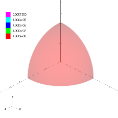
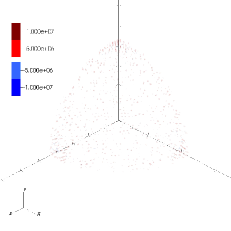
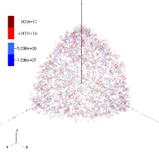
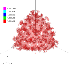
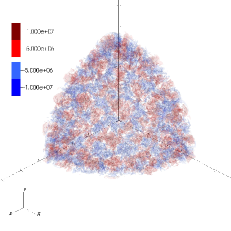
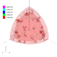
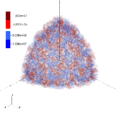
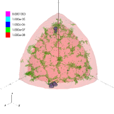
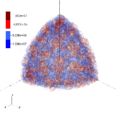
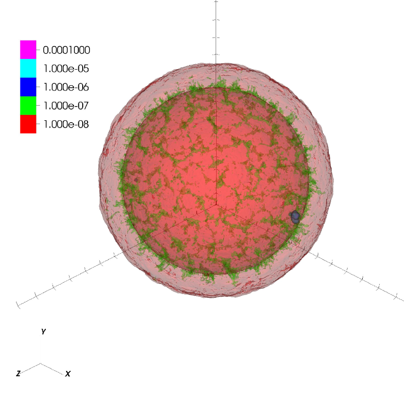
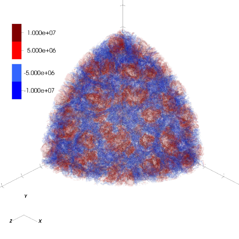
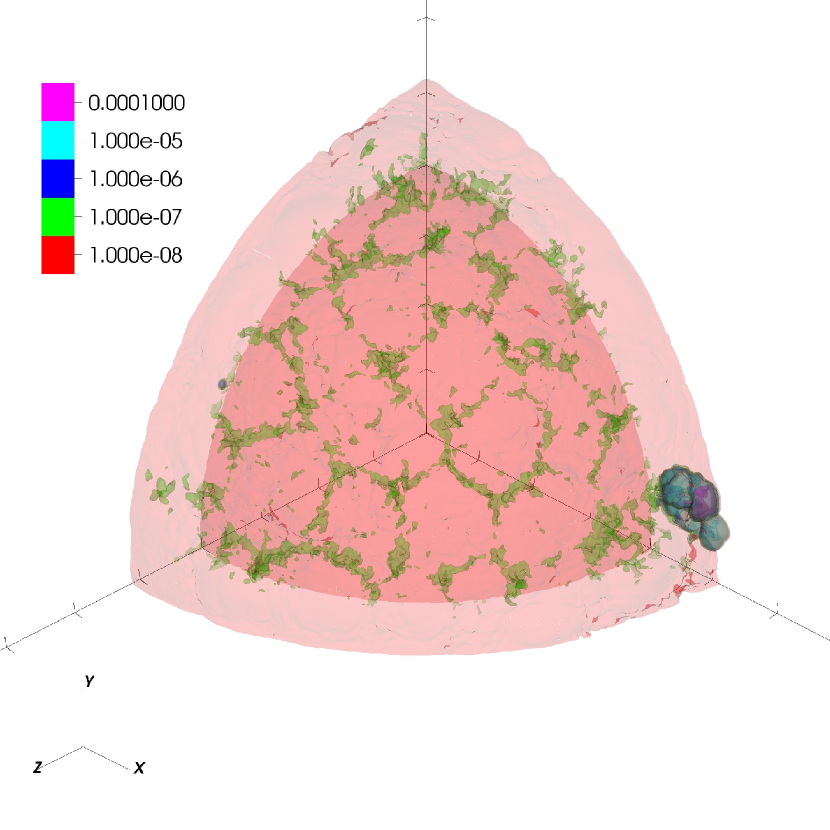
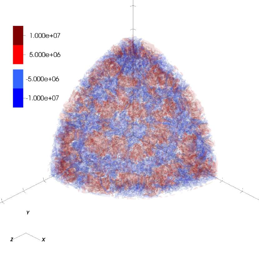
Figure 4 shows a time sequence for the reference calculation, with both the ${}^{16}\mathrm{O}$ abundance and radial velocity (red = outflow; blue = inflow) visualized. The development of the convection is clearly seen. By 80 s, the ${}^{16}\mathrm{O}$ synthesized at the base of the layer is distributed throughout the entire convective zone, and a clear top to the shell is seen. The radial velocity shows that the convection is divided into cells, with outflow regions surrounded by inflowing regions. Looking at the 80 s plot, there are approximately 6 such cells along the edge of the domain. The circumference of this edge is $\sim(\pi/2)5\times 10^{8}~{}\mathrm{cm}$ or $7.9\times 10^{8}~{}\mathrm{cm}$. This tells us that a convective cell has a diameter of approximately $1.3\times 10^{8}~{}\mathrm{cm}$. This is very close to the thickness of the convective layer ($\sim 10^{8}~{}\mathrm{cm}$ as seen in Figure 1). We note that the thickness of the convective layer is a function of the initial model, and we will explore other initial models in subsequent papers.

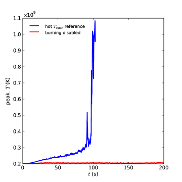
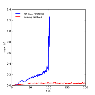
Figure 6 shows the peak temperature and peak Mach number as a function of time for this run. It is interesting to see that there are a number of failed ignitions toward the end—our suspicion is that the buoyant hotspots rise and cool via expansion faster than the rate at which energy is injected through reactions. This is supported by the relic plumes of ${}^{16}\mathrm{O}$ seen throughout Figure 4. A caveat to this behavior is that our network only continues to the production of ${}^{16}\mathrm{O}$. A more extensive reaction network might release enough energy for the first hot spot to fully ignite.

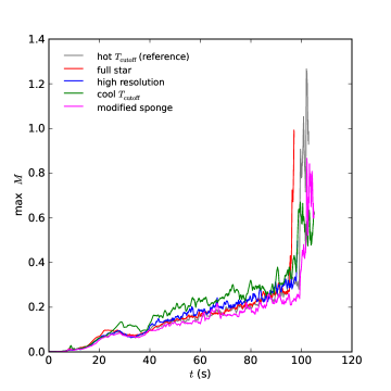
The Mach number panel in Figure 6 shows that the Mach number stays below $0.3$ for the bulk of the simulation. It is important to note that the efficiency metric for the low Mach number algorithm, the increase in time step over a compressible code, is not simply $1/M$ here. For a compressible simulation, the higher sound speed at the center of the star dominates the fluid velocities realized at the edge of the star. For these calculations, we evolve to $100~{}s$ in $\sim 2100$ time steps, giving an average $\Delta t_{\mathrm{lowMach}}\sim 0.05$. The peak sound speed in these models is $c_{s}=4.7\times 10^{8}~{}\mathrm{cm~{}s^{-1}}$. Taking the coarse grid spacing, $\Delta x=2.9\times 10^{6}~{}\mathrm{cm}$, the compressible time step for these models would be $\Delta t=\Delta x/c_{s}=6.2\times 10^{-3}~{}\mathrm{s}$—a factor of 8 smaller. Note that this doesn’t factor any of the fluid motions themselves into the compressible time step, which would only further reduce it. We also note that the early evolution begins with a much smaller Mach number, so the efficiency is greatest earlier in the evolution. Finally, once a hotspot ignites, the Mach number rises beyond the range of validity of the low Mach number approximation, and we would need to transition this problem to a compressible code to continue. Initial work on transitioning MAESTRO calculations to the compressible code CASTRO is shown in Almgren et al. (2010a).

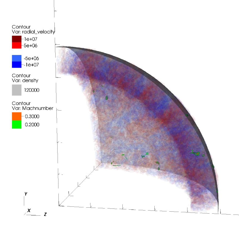
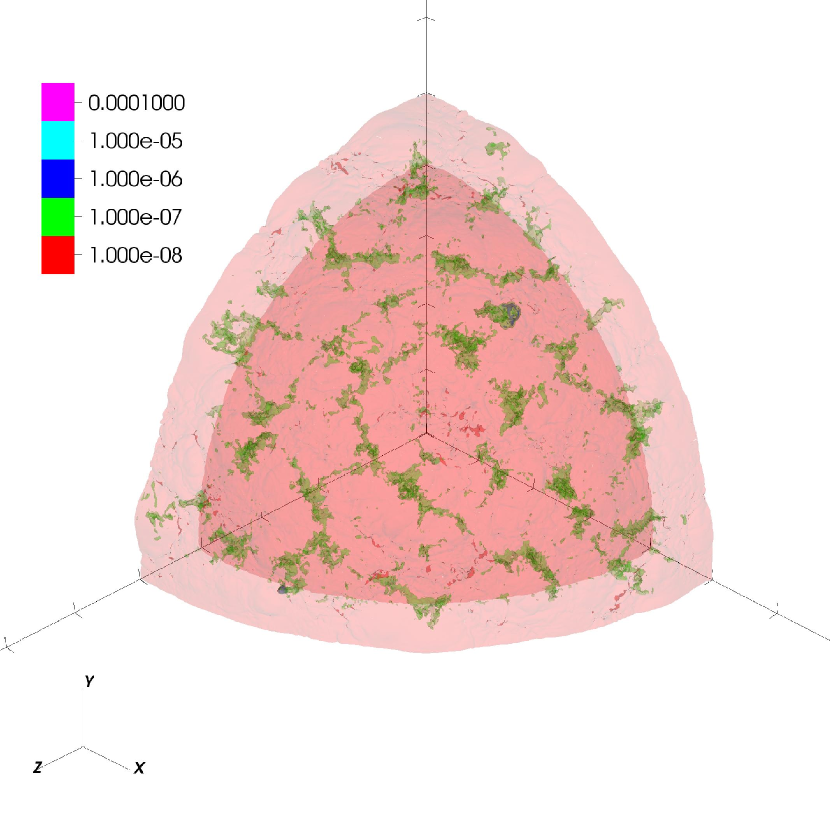
Figure 7 shows a side view of the convective layer for the reference calculation. We see that the convective layer is well bounded. The grey contour marks the density at which the sponge just begins to turn on—as designed, this is at the upper boundary of the convection. The orange and green contours show the regions where the Mach number is highest. We see that these regions are very small points, scattered throughout the layer, mostly near the top of the convective zone.

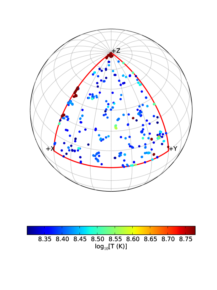
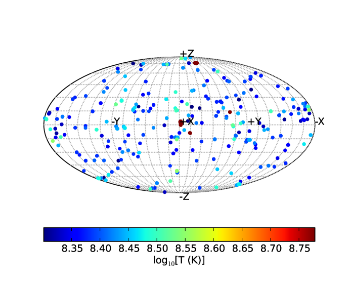
Figure 8 shows the location of the hottest point in the model (the hotspot) at each time step, colored by the logarithm of the temperature. We note that the time step changes over the course of the simulation (generally speaking, smaller time steps toward the end of the simulation). The points where ignition developed (seen, for example, as the ${}^{16}\mathrm{O}$ plumes in the final time snapshot in Figure 4) are shown in deep red. We notice that there seems to be a slight bias of ignition along the edges of the octant, where the flow can be confined by the geometry. We remind the reader that all simulations are done in Cartesian coordinates—the meridians and parallels drawn on the sphere are for guidance only.

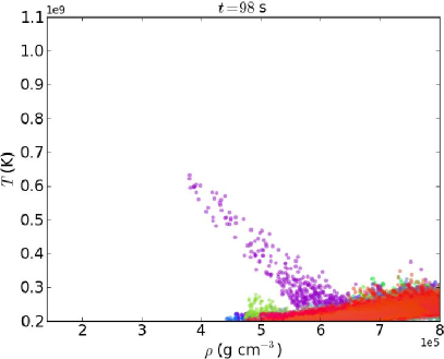
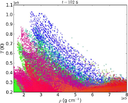
At a single snapshot, it is interesting to see how many hot plumes exist. Figure 9 shows the distribution of the hottest zones within the $\rho-T$ plane at two different times. The color coding of the dots indicate spatial location within the finest level of refinement on our grid—in particular the normalized $x,y,z$ coordinates of each zone are translated into $r,g,b$ colors for each data point. Groups of points of a similar color indicate simulation zones in close spatial proximity. The left plot, at $t=98$ s, shows in purple a single plume dominating the flow. There are a few smaller regions beginning to heat, the largest of which is the clump of green points. Only four seconds later ($t=102$ s), as seen in the right plot, the previously dominant plume (purple of the left plot) has cooled and redistributed its heat while several other distinct plumes have formed. This indicates that there are possibly several ignition regions, or at least several regions that are almost to runaway conditions once the dominant hot spot (blue points in this case) ignites. The extreme temperature sensitivity of the reaction rates makes it difficult to determine if these other “failed” ignition points would actually ignite.

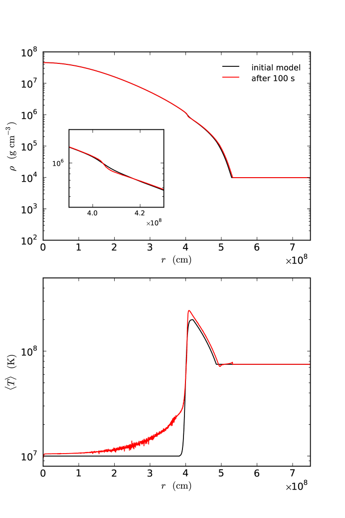
Finally, we can look at how much the atmosphere expanded over the course of the simulation. Figure 10 shows the base state density at the start of the reference hot-$T_{\mathrm{cutoff}}$ simulation and after 100 s of evolution, as well as the temperature averaged in a shell of constant radius at the start and end of the simulation. We see that a bit of expansion has taken place, smaller in magnitude but qualitatively the same as in our one-dimensional test. This supports the statement that we need to use the base state expansion in the hydrodynamics to accurately model the flow. The temperature plot shows that the heat generated by reactions has been transported throughout the convective layer. We note that there is heating below the convective layer, which may be due to the adjustment from the expansion of the base state on the adaptive grid. The magnitude of this heating is small and we do not expect it to affect the results. This is not seen in the case where we do not burn (next section).

3.2 Disabled Burning

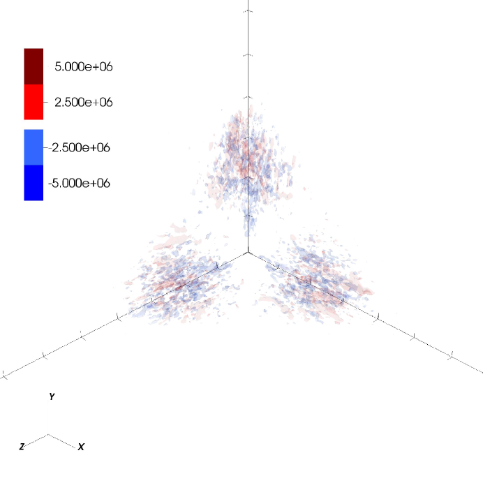
To demonstrate that the convective velocity field we see is driven by the reactions, and not due to the initial model’s temperature profile (Mocák et al., 2010) or discretization error, we run a test with the initial velocity perturbations, but burning disabled. The radial velocity field in this case is shown in Figure 11. We note that the range used in the contours is smaller than in Figure 4 to bring out the detail. We see no suggestion of the convective pattern that dominates in the burning calculations. Figure 6 shows the temperature and Mach number over the course of the simulations for the reference calculation with burning disabled. We see that the peak temperature stays right around the starting value of $2\times 10^{8}~{}\mathrm{K}$, as expected. The peak Mach number hits a plateau of $0.05$, driven by the artificial buoyancy introduced by the mapping error between the one-dimensional hydrostatic base state and the three-dimensional Cartesian state. This value does not seem to grow further. It is important to note that a compressible code would also see a velocity field generated in this test, again driven by the inability to exactly satisfy hydrostatic equilibrium numerically. Taken together, these figures indicate that the convective behavior described above arises due to the energy release from the reactions.

3.3 Full Star Simulation

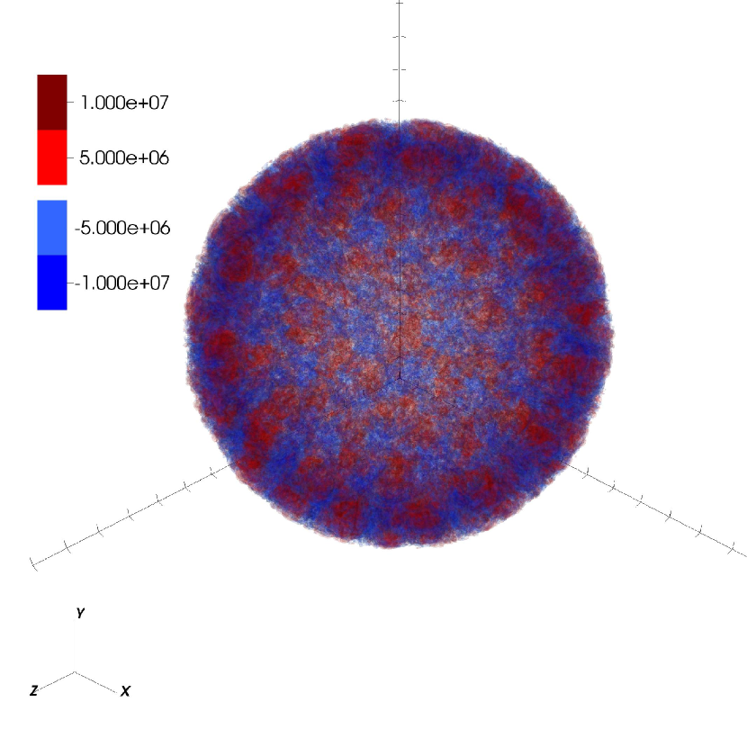
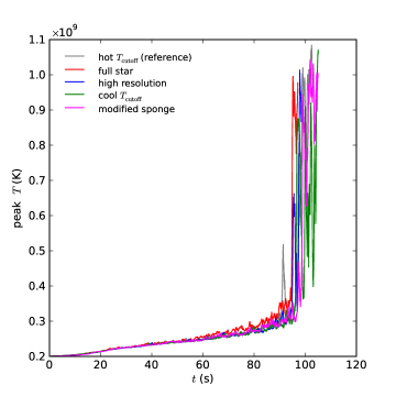
We run a single full-star calculation (using the hot-$T_{\mathrm{cutoff}}$ model) to assess the influence of the octant geometry on the general results described above. The resolution is the same, with the base grid now twice as large in each coordinate direction. The convective field is shown in Figure 12, and we see the same overall structure that appears in the octant simulations. The time-dependent peak temperature and Mach number (Figure 13) also agree well with the octant case. Figure 14 shows the hotspot location over time for this calculation. We see a uniform distribution of points over the sphere.

3.4 High-Resolution

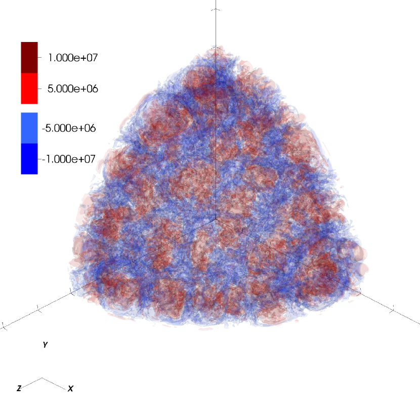
To understand the robustness of the convective features to resolution, we run a single case (hot-$T_{\mathrm{cutoff}}$ model) at twice the resolution. This is accomplished by doubling the number of zones in each direction on the coarse grid. Figure 15 shows the convective field for this simulation, in which the overall structure agrees with that of the standard-resolution simulations. The time-dependent peak temperature and Mach number for this run (Figure 13) again show excellent agreement with the standard-resolution runs. This gives us confidence that we are sufficiently numerically converged.

3.5 Cooler Initial Model

The corresponding images for the cool-$T_{\mathrm{cutoff}}$ simulation near the point of ignition are shown in Figure 16. There is a strong qualitative similarity with the hot-$T_{\mathrm{cutoff}}$ run, indicating that the structure of the convection is insensitive to the details of the top of the convective zone. We also see the expected behavior that the hot-$T_{\mathrm{cutoff}}$ model has a lower peak $M$ than the cool-$T_{\mathrm{cutoff}}$ model because of the higher sound speed at the edge of the star. This suggests that the peak Mach number occurs at the edge of the star, outside of the convective region.

3.6 Effect of Cutoff Densities and Sponging

In the simulations above, we chose the sponging parameters such that the sponging begins just at the top of the convective layer. Here we explore the sensitivity of that choice by turning the sponge on lower—we now set $\rho_{\mathrm{md}}=\rho_{\mathrm{anelastic}}=10^{5}~{}\mathrm{g~{}cm^{-3}}$. Additionally, we decrease the timescale over which the sponging acts by changing $\kappa=10~{}\mathrm{s^{-1}}$ to $\kappa=100~{}\mathrm{s^{-1}}$ (see Almgren et al. 2008).

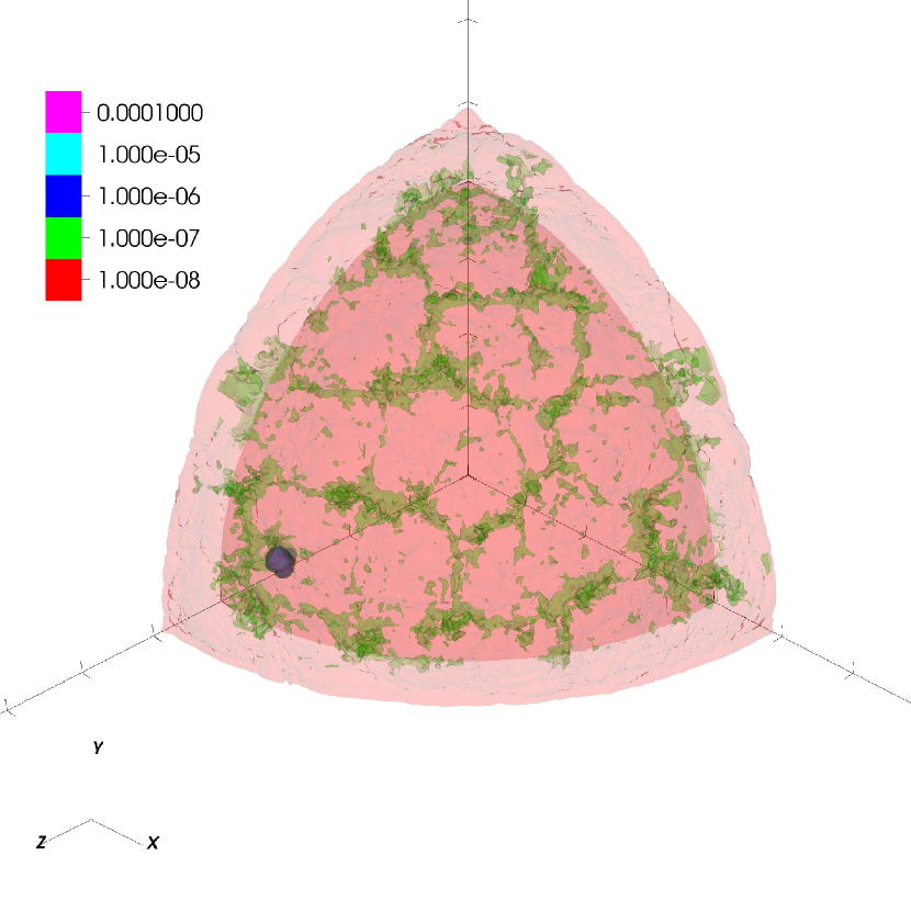
Figure 17 shows the structure of the convective field. We notice that the radial extent appears slightly diminished compared to the previous simulations, owing to the more aggressive sponging. However, the overall pattern of convective cells appears consistent with the other cases. The trends of peak temperature and Mach number are shown in Figure 13, and exhibit a slightly lower peak Mach number as the reference simulation due to the more aggressive sponging. These comparisons show that the convective behavior is not strongly dependent on how we treat the top of the convective layer.

4 Conclusions and Discussion

The main goal of the present paper is to serve as a proof-of-concept that the low Mach number methodology can be applied to shell burning on the surface of white dwarfs. This is the first application of MAESTRO where we have had off-center heating with an expanding, self-gravitating hydrostatic state. We demonstrated that efficient three-dimensional models of the convective flow leading up to the ignition of a burning front in a helium layer on the surface of a white dwarf are possible. We explored the sensitivity of our results to a variety of factors and showed that the convective features realized are robust. The octant calculations are inexpensive to run (requiring only about 40,000 CPU hours on the OLCF jaguar machine, using 128 MPI tasks with 8 OpenMP threads per task). This suggests that a parameter study of progenitor models is feasible—this will be the focus of a follow-on paper. There is a wide variety of potential models—varying white dwarf masses and helium envelopes. The conditions at the base of the helium layer will vary across these different models, so some models may be more amenable to our methodology than others. This needs to be explored on a case-by-case basis. For instance, we expect that low mass shells and lower mass white dwarfs would have slower dynamics.

Future work will focus on better understanding the conditions in the helium layer leading up to ignition. Open scientific questions that we wish to understand are whether the ignition occurs in a manner that is amenable to a detonation—this is a key requirement for the sub-Chandrasekhar explosion models. Also of interest is whether ignition can arise in multiple disjoint points on the surface of the white dwarf. Studying this will require either enhancements to the low Mach number model (i.e. the addition of long wavelength acoustics) or feeding MAESTRO models into a compressible hydrodynamics code. Finally, the models presented here started rather late in the evolution, but it is easy to start with cooler models to see more of the ramp up to ignition. This earlier evolution will take place at lower Mach numbers.

Figure 1: The initial model. The solid lines are for the cooler cutoff model ($T_{\mathrm{cutoff}}=5\times 10^{7}$ K) and the dashed lines are for the hotter cutoff model ($T_{\mathrm{cutoff}}=7.5\times 10^{7}$ K). The vertical lines indicate the start of the sponge (leftmost), the anelastic cutoff (center), and the base cutoff density (rightmost), again with solid for the cooler cutoff model and dashed for the hotter cutoff model.

Figure 2: A test of the base state expansion algorithm. The initial model is shown as the dotted line (for the choice $\rho_{\mathrm{cutoff}}=10^{4}~{}\mathrm{g~{}cm^{-3}}$). The compressible solution by the CASTRO code is shown as the black line, and three MAESTRO solutions are shown, with varying $\rho_{\mathrm{cutoff}}$. We see very good agreement across the board between MAESTRO and CASTRO, with the two lowest cutoff densities showing the best match.

Table 1: Cutoff parameter values

parameter	cool-$T_{\mathrm{cutoff}}$ model	hot-$T_{\mathrm{cutoff}}$ model
$\rho_{\mathrm{cutoff}}$	$10^{4}~{}\mathrm{g~{}cm^{-3}}$	$10^{4}~{}\mathrm{g~{}cm^{-3}}$
$\rho_{\mathrm{md}}$	$3\times 10^{4}~{}\mathrm{g~{}cm^{-3}}$	$6\times 10^{4}~{}\mathrm{g~{}cm^{-3}}$
$f_{\mathrm{sp}}$	$2.0$	$2.0$
$\rho_{\mathrm{anelastic}}$	$3\times 10^{4}~{}\mathrm{g~{}cm^{-3}}$	$6\times 10^{4}~{}\mathrm{g~{}cm^{-3}}$

Figure 3: A representative 2-level grid used for the simulations.

Figure 4: Time sequence of the ${}^{16}\mathrm{O}$ abundance (left) and radial velocity (right) for the hot-$T_{\mathrm{cutoff}}$ reference simulation shown at 20, 40, 60, 80, and 100 s. The tick marks are spaced $10^{8}$ cm apart. The ${}^{16}\mathrm{O}$ sequence highlights the extent of the convective region well—by 80 s, there is a well-defined upper surface to the convective zone. The radial velocity (CGS units); red=outflow, blue=inflow) shows a characteristic “granulation” pattern, making the distinct convective cells stand out.

Figure 4: Time sequence continued.

Figure 6: Peak temperature and Mach number as a function of time for our reference calculation (hot-$T_{\mathrm{cutoff}}$) and the same calculation with burning disabled.

Figure 7: Side view of the convective field of the hot-$T_{\mathrm{cutoff}}$ reference run at 95 s. All contours are in CGS units. The tick marks are $10^{8}$ cm apart. The grey density contour marks the surface where the sponging just begins to turn on—we see that the convection is entirely below this surface. The orange and green contours show the locations where the Mach number is highest.

Figure 8: Location of the hottest point at each time step in the reference simulation, colored according to temperature. The red boundary shows the bounds of the octant modeled.

Figure 9: Distribution in the $\rho-T$ plan of the hottest zones in the finest level; the left plot shows a snapshot at $t=98$ s and the right plot shows a snapshot at $t=102$ s. Colors represent a proxy for spatial location. Within four seconds, the single dominant plume in the left plot is washed away and replaced by several distinct hot regions of which the group of blue zones reach runaway conditions.

Figure 10: Base state density and lateral average of the temperature at the start and end of the reference hot-$T_{\mathrm{cutoff}}$ simulation.

Figure 11: Radial velocity (CGS units) for the “no burning” test model after 197 s. Note: the range on the contours is smaller here than in Figure 4 to bring out detail. The tick marks are $10^{8}$ cm apart. We see no evidence of the convective field structure. Instead, the random velocities here are driven by discretization error.

Figure 12: ${}^{16}\mathrm{O}$ abundance (left) and radial velocity (right; CGS units) for the fullstar hot-$T_{\mathrm{cutoff}}$ model at 96 s—just at the point where we are igniting. The tick marks are $10^{8}$ cm apart. The overall convective structure compares well to the octant simulations.

Figure 13: Peak temperature and Mach number as a function of time for the various supporting calculations: full star, high-resolution, cool-$T_{\mathrm{cutoff}}$ model, and stronger sponging. The reference hot-$T_{\mathrm{cutoff}}$ calculation is also shown. We see that the trends for all quantities are the same for all runs, indicating that our simulation is converged in resolution, and the octant is a reasonable model for the energetic evolution, and that the treatment at the outer radius of the convective region is not critically important.

Figure 14: Location of the hottest point at each time step for the full-star, hot-$T_{\mathrm{cutoff}}$ calculation.

Figure 15: ${}^{16}\mathrm{O}$ abundance (left) and radial velocity (right; CGS units) for the high-resolution hot-$T_{\mathrm{cutoff}}$ near the point of ignition (98 s). The tick marks are $10^{8}$ cm apart. The overall structure compares well to the standard-resolution hot-$T_{\mathrm{cutoff}}$ simulation.

Figure 16: ${}^{16}\mathrm{O}$ abundance (left) and radial velocity (right; CGS units) for the cool-$T_{\mathrm{cutoff}}$ model at 100 s. The tick marks are $10^{8}$ cm apart. The overall structure compares well to the hot-$T_{\mathrm{cutoff}}$ simulation.

Figure 17: ${}^{16}\mathrm{O}$ abundance (left) and radial velocity (right) for the hot-$T_{\mathrm{cutoff}}$ run with more aggressive sponging at the top of the convective layer. Shown at 100 s. The tick marks are $10^{8}$ cm apart. Again, we see good agreement with the other cases.

References

- Alastuey & Jancovici (1978) Alastuey, A., & Jancovici, B. 1978, ApJ, 226, 1034
- Almgren et al. (2010a) Almgren, A., et al. 2010a, ArXiv e-prints, 1008.2801
- Almgren et al. (2008) Almgren, A. S., Bell, J. B., Nonaka, A., & Zingale, M. 2008, ApJ, 684, 449
- Almgren et al. (2006) Almgren, A. S., Bell, J. B., Rendleman, C. A., & Zingale, M. 2006, ApJ, 637, 922
- Almgren et al. (2010b) Almgren, A. S., et al. 2010b, Astrophysical Journal, 715, 1221, astro-ph/1005.0114
- Caughlan & Fowler (1988) Caughlan, G. R., & Fowler, W. A. 1988, Atomic Data and Nuclear Data Tables, 40, 283, see also http://www.phy.ornl.gov/astrophysics/data/cf88/index.html
- Fink et al. (2007) Fink, M., Hillebrandt, W., & Röpke, F. K. 2007, Astronomy and Astrophysics, 476, 1133, 0710.5486
- Fink et al. (2010) Fink, M., Roepke, F. K., Hillebrandt, W., Seitenzahl, I. R., Sim, S. A., & Kromer, M. 2010, Astronomy and Astrophysics, 514, A53+
- García-Senz et al. (1999) García-Senz, D., Bravo, E., & Woosley, S. E. 1999, A&A, 349, 177
- Garnett (1997) Garnett, D. R. 1997, Nuclear Physics A, 621, 27
- Graboske et al. (1973) Graboske, H. C., Dewitt, H. E., Grossman, A. S., & Cooper, M. S. 1973, ApJ, 181, 457
- Hoeflich & Khokhlov (1996) Hoeflich, P., & Khokhlov, A. 1996, ApJ, 457, 500, arXiv:astro-ph/9602025
- Hoeflich et al. (1996) Hoeflich, P., Khokhlov, A., Wheeler, J. C., Phillips, M. M., Suntzeff, N. B., & Hamuy, M. 1996, ApJ, 472, L81, arXiv:astro-ph/9609070
- Itoh et al. (1979) Itoh, N., Totsuji, H., Ichimaru, S., & Dewitt, H. E. 1979, ApJ, 234, 1079
- Kromer et al. (2010) Kromer, M., Sim, S. A., Fink, M., Röpke, F. K., Seitenzahl, I. R., & Hillebrandt, W. 2010, ApJ, 719, 1067, 1006.4489
- Livne (1990) Livne, E. 1990, ApJ, 354, L53
- Livne & Glasner (1990) Livne, E., & Glasner, A. S. 1990, ApJ, 361, 244
- Malone et al. (2011) Malone, C. M., Nonaka, A., Almgren, A. S., Bell, J. B., & Zingale, M. 2011, ApJ, 728, 118, 1012.0609
- Mocák et al. (2010) Mocák, M., Campbell, S. W., Müller, E., & Kifonidis, K. 2010, A&A, 520, A114, 1003.3646
- Nonaka et al. (2010) Nonaka, A., Almgren, A. S., Bell, J. B., Lijewski, M. J., Malone, C. M., & Zingale, M. 2010, ApJS, 188, 358
- Nonaka et al. (2012) Nonaka, A., Aspden, A. J., Zingale, M., Almgren, A. S., Bell, J. B., & Woosley, S. E. 2012, ApJ, 745, 73, 1111.3086
- Nugent et al. (1997) Nugent, P., Baron, E., Branch, D., & Fisher, A. andHauschildt, P. H. 1997, ApJ, 485, 812, arXiv:astro-ph/9612044
- Shen et al. (2010) Shen, K. J., Kasen, D., Weinberg, N. N., Bildsten, L., & Scannapieco, E. 2010, ApJ, 715, 767, astro-ph/1002.2258
- Sim et al. (2010) Sim, S. A., Röpke, F. K., Hillebrandt, W., Kromer, M., Pakmor, R., Fink, M., Ruiter, A. J., & Seitenzahl, I. R. 2010, ApJ, 714, L52, astro-ph/1003.2917
- Timmes (2008) Timmes, F. X. 2008, http://cococubed.asu.edu/code_pages/eos.shtml
- Timmes & Swesty (2000) Timmes, F. X., & Swesty, F. D. 2000, ApJS, 126, 501
- Townsley et al. (2012) Townsley, D. M., Moore, K., & Bildsten, L. 2012, ApJ, 755, 4, 1205.6517
- Weaver & Woosley (1993) Weaver, T. A., & Woosley, S. E. 1993, Phys. Rep., 227, 65
- Weaver et al. (1978) Weaver, T. A., Zimmerman, G. B., & Woosley, S. E. 1978, ApJ, 225, 1021
- Wiggins & Falle (1997) Wiggins, D. J. R., & Falle, S. A. E. G. 1997, MNRAS, 287, 575
- Wiggins et al. (1998) Wiggins, D. J. R., Sharpe, G. J., & Falle, S. A. E. G. 1998, MNRAS, 301, 405
- Woosley & Kasen (2011) Woosley, S. E., & Kasen, D. 2011, ApJ, 734, 38, 1010.5292
- Woosley & Weaver (1994) Woosley, S. E., & Weaver, T. A. 1994, ApJ, 423, 371
- Zingale et al. (2009) Zingale, M., Almgren, A. S., Bell, J. B., Nonaka, A., & Woosley, S. E. 2009, ApJ, 704, 196
- Zingale et al. (2011) Zingale, M., Nonaka, A., Almgren, A. S., Bell, J. B., Malone, C. M., & Woosley, S. E. 2011, ApJ, 740, 8