The Degeneracy Problem in Non-Canonical Inflation
Damien A. Easson1,† and Brian A. Powell2,⋆
1 Department of Physics & School of Earth and Space Exploration & Beyond Center
Arizona State University, Tempe, AZ 85287-1504
2 Institute for Defense Analyses, Alexandria, VA 22311
Abstract
While attempting to connect inflationary theories to observational physics, a potential difficulty is the degeneracy problem: a single set of observables maps to a range of different inflaton potentials.
Two important classes of models affected by the degeneracy problem are canonical and non-canonical models, the latter marked by the presence of a non-standard kinetic term that generates observables beyond the scalar and tensor two-point functions on CMB scales. The degeneracy problem is manifest when these distinguishing observables go undetected. We quantify the size of the resulting degeneracy in this case
by studying the most well-motivated non-canonical theory having Dirac-Born-Infeld Lagrangian. Beyond the scalar and
tensor two-point functions on CMB scales, we then consider the possible detection of equilateral non-Gaussianity at Planck-precision and a measurement of
primordial gravitational waves from prospective space-based laser interferometers. The former detection breaks the degeneracy with canonical inflation but results in poor reconstruction prospects, while the latter measurement enables a determination of which, while not breaking the degeneracy, can be shown to greatly improve the non-canonical reconstruction.
†easson@asu.edu
⋆brian.powell007@gmail.com
1 Introduction
The most successful model of early universe cosmology is the inflationary universe paradigm [1, 2]. The general predictions of single field slow roll inflation, including a large, flat universe with correlations between fluctuations in matter and radiation and a nearly scale-invariant spectrum of perturbations, are all corroborated by the data; however, it is notoriously difficult to make any detailed statements about the fundamental mechanism behind the accelerated expansion. In the simple case of single field canonical inflation, the amplitudes of the scalar and tensor power spectra on CMB scales uniquely map to the parameters of the inflationary Lagrangian. However, the inflaton need not be canonically normalized, nor need it be the primary source of primordial perturbations. There might even be several inflaton fields cooperatively driving inflation. In these cases, the unique mapping of observables to the Lagrangian is threatened – distinct inflation models from different classes can give rise to the same set of observables, to within experimental precision. This is known as the degeneracy problem. Two broad classes of theories which contribute to the degeneracy problem are theories in which degrees of freedom other than the inflaton serve as the source for primordial curvature perturbations, e.g. the curvaton scenario, and theories where the field dynamics are determined by terms in the Lagrangian other than, or in addition to, the scalar potential, , e.g. models with non-canonical kinetic terms. The former source of degeneracy – that arising from curvatons – was investigated in detail in a companion paper to the present work, Ref. [4]. In this paper, we examine the degeneracy problem in the context of non-canonical inflation, selecting the Dirac-Born-Infeld (DBI) model as a prototype.
Exact degeneracies only exist between certain classes of models, for example, between canonical minimally and non-minimally coupled fields111This degeneracy does not exist between minimally and non-minimally coupled non-canonical models [5].. Other broad classes, like curvaton and non-canonical models, generically give rise to distinguishing observables beyond the scalar and tensor power spectra, and , like isocurvature modes and/or non-Gaussianities. Just as and determine in canonical inflation, in DBI an additional function, the sound speed , contributes to the reconstruction. When , large equilateral non-Gaussianities are generated, and so can be measured and used, along with and , to reconstruct in DBI inflation. In practice, the degeneracy problem is manifest when these additional observables are not detected, whether due to experimental limitations or the specifics of the scenario. Planck will fail to detect if : then, not only would canonical inflation () be consistent with such an observation, but a range of other non-canonical model potentials that result from varying within the range would be equally consistent [24]. The degeneracy problem is bad not only because we do not know the underlying type of theory (e.g. canonical or non-canonical), but because the resulting potential reconstruction is generally much worse relative to that possible under the assumption of canonical inflation for the same set of observables.
In this paper, we perform Monte Carlo reconstructions of for a range of observational outcomes. We first consider the worst-case scenario in which no additional distinguishing observable, namely, equilateral non-Gaussianity, is detected. We then examine how positive detections of and a possible scale-dependence of the three-point function, , at Planck-precision affect the reconstruction. While these observations break the degeneracy in favor of a model like DBI inflation, our reconstruction of is limited by the precision with which these observables are measured. Generally, we find that the DBI reconstruction is worse than the reconstructed canonical model generating the equivalent and . That is, unless, it is possible to obtain a quality measurement of , the tensor spectral index. Such a measurement might be possible through a detection of primordial gravitational waves with future space-based laser interferometers such as the Big-Bang-Observer (BBO) and Japan’s planned DECIGO experiment. In this case, even though the degeneracy is unbroken, the quality of the DBI reconstruction is greatly improved, with the range of consistent potentials only slightly larger than the range of canonical potentials. This is because the modified consistency relation relating to the tensor/scalar ratio, , is used to replace the undetermined for in the reconstruction equations. This finding, described in detail in §3.4.3, was originally discussed along with a similar result applicable to curvatons in [3]. 222Note, the test of the inflationary consistency relations play a crucial role in helping to distinguish between different inflationary models, see e.g. [8].
This paper is organized as follows. In §2, we outline the potential reconstruction program for non-canonical inflationary models. §3 provides the motivation for considering DBI models in the context of D-brane inflation in string theory and presents the Monte Carlo analysis. §4 is devoted to a brief discussion of our results.
2 Potential Reconstruction in Non-Canonical Inflation
Methods for reconstructing a general inflationary Lagrangian were developed in [6] and encompass a broad range of theories, including non-canonical models in which the kinetic term in the Lagrangian is not canonically normalized,
| (2.1) |
where . Models of this form were first popularized in the context of k-inflation [7], in which higher-derivative kinetic terms drive inflation in the absence of a potential. More recently, non-canonical inflation has found relevance in models constructed from string theory, such as D-brane inflation [9, 10, 11, 12, 13, 14] and the dynamical regime known as DBI inflation [15, 16]. While many of these constructions generically involve multiple fields, we restrict our analysis to single field models.
From the Friedmann and continuity equations,
| (2.2) | |||||
| (2.3) |
one obtains the Hamilton-Jacobi equation [6],
| (2.4) |
where . Canonical inflation is recovered for , giving
| (2.5) |
Evidently, in canonical theories, completely governs the inflationary trajectory and determines the scalar potential . In contrast, the non-canonical trajectory is characterized by two functions:
| (2.6) | |||||
| (2.7) |
resulting in two separate hierarchies of flow parameters. The first, called the H-tower,
| (2.8) | |||||
generalizes the canonical flow parameters [17], recovered by taking . The second is unique to non-canonical theories and is called the -tower,
| (2.10) |
With both and the non-canonical kinetic term governing the inflationary dynamics in these theories, cosmological observations must be used to disentangle the physical effects of these two functions in order to successfully reconstruct them. This is the challenge investigated in this paper.
While many characteristics of non-canonical inflation are model dependent, we focus on the conservative models where perturbations propagate relative to the homogeneous background at speeds less than that of light. 333For a more general treatment see [18]. From Eqs. (2.2-2.3), the hydrodynamical sound speed is given by
| (2.11) |
where . This is in contrast to canonical inflation, for which and . Fluctuations that travel with speeds are non-Gaussian, a property that is not related directly to the scalar potential; these observations will be important for distinguishing the effects of from those of the kinetic term. In the next section, we investigate reconstruction in the context of a prototypical non-canonical model – DBI inflation.
3 Case Study: Reconstruction in DBI Inflation
3.1 The Scenario and the Power Spectrum
A theoretically well-motivated example of non-canonical inflation arises from D-brane inflation in string theory. The most well-studied framework is based on Calabi-Yau flux compactifications of Type IIB string theory [19], in which the inflaton parameterizes the motion of a probe brane relative to an anti-brane at the tip of a warped throat geometry. This geometry is given by the line element [20],
| (3.12) |
where the internal space is a cone over the base manifold . The throat coordinate determines the inflaton field, , where is the tension of the brane: in UV models the probe is a D3-brane falling towards a stack of anti-D3 branes at the tip of the throat, while in IR models [21] the probe is an anti-D3-brane being pushed up the throat away from the stack. In either case, the equation of motion of the probe brane is obtained from the DBI Lagrangian [15],
| (3.13) |
where is determined by the warp factor . The non-canonical kinetic term in Eq. (3.13) enforces an effective speed limit on the inflaton field, with the result that ‘slow roll’ inflation can be achieved even in the presence of steep potentials [16]. From the AdS/CFT correspondence, the speed limit on the field space arises from the fact that the probe brane must travel subluminally; in analogy with special relativity, we define the -factor,
| (3.14) |
From the Lagrangian Eq. (3.13), we find and using this in Eq. (2.11) gives . The causality constraint on the probe brane not only imposes a speed limit on the field space, but also reduces the propagation speed of fluctuations.
The Friedmann equation follows from Eq. (3.13),
| (3.15) |
and gives
| (3.16) |
The -factor Eq. (3.14) then becomes
| (3.17) |
From these results the Hamilton-Jacobi equation, Eq. (2.4), can be obtained for DBI inflation,
| (3.18) |
With , we can use Eqs. (2.8) and (2) to write down the first few derivatives of the potential,
| (3.19) | |||||
| (3.20) | |||||
where . An important distinction should be made between the DBI reconstruction and that of the curvaton carried out in the companion analysis [4]: the curvaton does not modify the inflationary dynamics, it serves only as a means of generating the primordial density perturbation. In other words, the same inflationary Lagrangian will generate different spectra depending on whether a curvaton is present or not – a degeneracy with single field models develops if we are unable to detect its presence. In contrast, DBI inflation is dynamically distinct from canonical inflation, and so different observables necessarily arise from different Lagrangians. However, a degeneracy therefore develops if the observables characteristic of non-canonical inflation are not detected.
We proceed by connecting the potential coefficients to cosmological observables. In theories of inflation with an arbitrary speed of sound, the amplitude of curvature perturbations at first order in slow roll is [22]:
| (3.21) |
where the amplitude is evaluated at sound horizon-crossing: . On the other hand, the tensor amplitude,
| (3.22) |
is evaluated at Hubble crossing, , because gravitational waves propagate at the speed of light. If the difference in sound horizon crossing and Hubble crossing times is small for a given wavenumber, , then the tensor/scalar ratio is well approximated by the expression,
| (3.23) |
This is a fair assumption during slow roll [23, 24]. The scalar spectral index exhibits a dependence on the time rate of change of ,
| (3.24) |
while the tensor spectral index is the same as in canonical inflation,
| (3.25) |
Working to lowest order in slow roll and assuming a constant speed of sound (), Eqs. (3.22), (3.23), and (3.24) can be inverted to obtain the potential coefficients Eqs. (3.1-3.20) in terms of the spectrum observables,
| (3.26) | |||||
In additional to the spectrum observables, the potential depends on the value of the -factor.444All expressions for DBI inflation reduce to those of canonical inflation when , , . Despite the above-mentioned formal distinction between the curvaton and DBI reconstructions, the two cases are treated in a similar manor: determination of requires observations of more than simply the adiabatic density perturbation and tensor spectra. In the case of curvatons, the amplitude of the curvaton fluctuation needs to be measured; in the case of DBI inflation, the -factor (equivalently, the sound speed ) must be constrained. Equations (3.1-3.26) are only approximate and we will conduct a more rigorous reconstruction in a later section.
3.2 Non-Gaussianity
The non-canonical kinetic term in the DBI Lagrangian Eq. (3.13) generically leads to the production of primordial non-Gaussianity. In contrast to curvaton and general multifield models, the large non-Gaussianity arises from the three-point correlator of the field fluctuations, , rather than the nonlinear interaction of the field and curvature perturbations. In the DBI model, the strongest correlation arises amongst modes of comparable wavenumber at the horizon, and so is evaluated in the equilateral limit, [16, 25],
| (3.27) |
Being of a different form in Fourier space than local-type non-Gaussianity (for which ), a measurement of the shape of non-Gaussianities offers the possibility of distinguishing DBI inflation from the curvaton and other theories that generate local non-Gaussianities, like modulated reheating. The non-Gaussianities produced in DBI inflation can be very large in the DBI limit, , in which the field is rolling relativistically, . The equilateral-type non-Gaussianities are less constrained by current data than the local-type: WMAP7 gives at 95% CL [26]. This is due to the fact that for a given amplitude, the distribution of local-type fluctuations is more significantly skewed than the equilateral distribution. As a result, future projections are also not as limiting as for local non-Gaussianities: Planck should achieve at 68% CL [27]. However, in contrast to the non-Gaussianities produced in the curvaton scenario, a measurement of completely determines the additional degree of freedom in the reconstruction, and a detection of higher-order statistics like the trispectrum is unnecessary.
For completeness we mention that it is possible that the amplitude of non-Gaussianities generated during DBI inflation varies with scale [28], so that , with the spectral index defined as
| (3.28) |
The projected 1 error on expected from Planck is [29]
| (3.29) |
with CMBPol expected to improve on this limit by around a factor of two. We consider Planck sensitivity detections for non-Gaussianity in this paper as the factor of two improvement will not be significant enough to strongly affect the results. We investigate the effect of a detection of non-Gaussianities – both the amplitude and the scale dependence – on reconstruction in §3.4.2.
3.3 Gravitational Waves
The non-standard sound speed that is the hallmark of DBI inflation results in the modified scalar spectrum given by Eq. (3.21). However, since gravitational waves propagate at the speed of light, the spectrum of tensor modes is still proportional to the energy scale of inflation, Eq. (3.22). This results in a modified consistency relation,
| (3.30) |
A reliable determination of the consistency relation requires a quality measurement of . Concept studies of future space-based laser interferometers designed to measure the primordial gravitational wave signal on small scales ( Hz) have yielded promising results. Two proposals, the Big Bang Observer (BBO) [30] and Deci-hertz Interferometer Gravitational Wave Observatory, (DECIGO) [31], will detect gravitational waves if B modes on CMB scales give and , respectively – a substantial part of the observable parameter space. These probes are intended to enable a determination of with a precision surpassing future CMB probes: BBO should give a 65% CL of while DECIGO might achieve or better [32, 33]. We simulate the effect that such a detection has on DBI reconstruction in the next section.
3.4 Monte Carlo Analysis
The inversion from the observable parameter space to the flow space enables one to write the inflaton potential in terms of observables as in Eq. (3.1). However, this process is only tractable if the observables are written to lowest order in the flow parameters (c.f. Eqs. (3.23) and (3.24)). A more accurate and efficient method for reconstruction at higher order can be accomplished using Monte Carlo methods [34, 35, 36]. One begins with the flow parameters and for each stochastically sampled initial condition, solves the flow equations [37],
| (3.31) | |||||
| (3.32) | |||||
| (3.33) | |||||
| (3.34) | |||||
| (3.35) | |||||
| (3.36) | |||||
| (3.37) | |||||
| (3.38) | |||||
| (3.39) | |||||
| (3.40) | |||||
| (3.41) |
where the system is truncated by taking and is the number of efolds before the end of inflation. Taken as a time variable, over the course of inflation. The solution to these equations is an exact DBI inflationary trajectory with potential determined from Eq. (3.1). The observables can also be determined from the flow parameters and those models which agree with observations can be selected out. We retain only those models that support sufficient inflation to generate the CMB anisotropies, , and we work to -order in the -tower and -order in the -tower. We draw the -tower parameters from the initial ranges
| (3.42) |
and the -tower from the ranges: , , . We are therefore including in our analysis models with a time-dependent speed of sound; from Eq. (2.7) with , the inverse sound speed is quadratic in . From Eq. (3.17), there is then some freedom in the form of the warp factor, .
We choose so that the largest length scales of interest correspond to the quadrupole. Since density perturbations freeze out when and tensors when , care must be taken when matching the scale to the e-fold number, . For density perturbations, the scale at horizon crossing is determined by solving along with the flow equations, and for each acceptable solution we calculate the observables at [25, 38]
| (3.43) |
where , and is the Euler-Mascheroni constant. For tensor perturbations, the scale at horizon crossing is given by the usual relation , with the following observables calculated at [39],
| (3.44) |
We then calculate the tensor/scalar ratio from .
We perform the above-described flow analysis for canonical inflation as well, obtained with the above method by taking , . The approach taken here is analogous to that carried out in [4] for curvatons: the results obtained there for single field field inflation are identical to those obtained here for canonical inflation, and the results that we present here for DBI models can also be directly compared against our findings for curvatons in [4]. We now present results for different observational outcomes.
3.4.1 No Detection of Non-Gaussianity
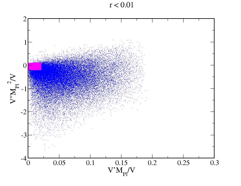
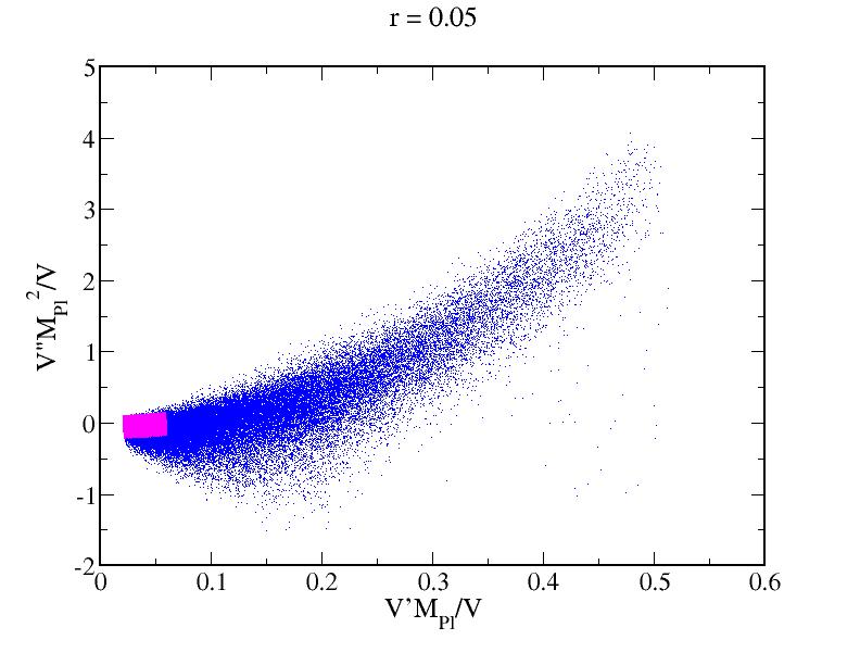
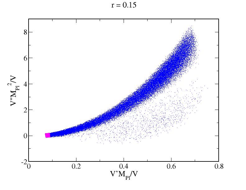
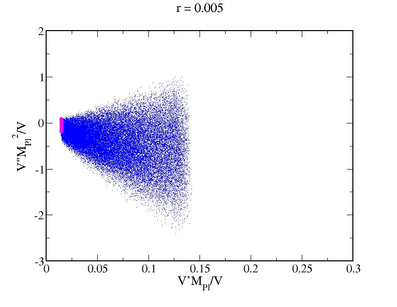
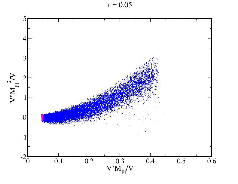
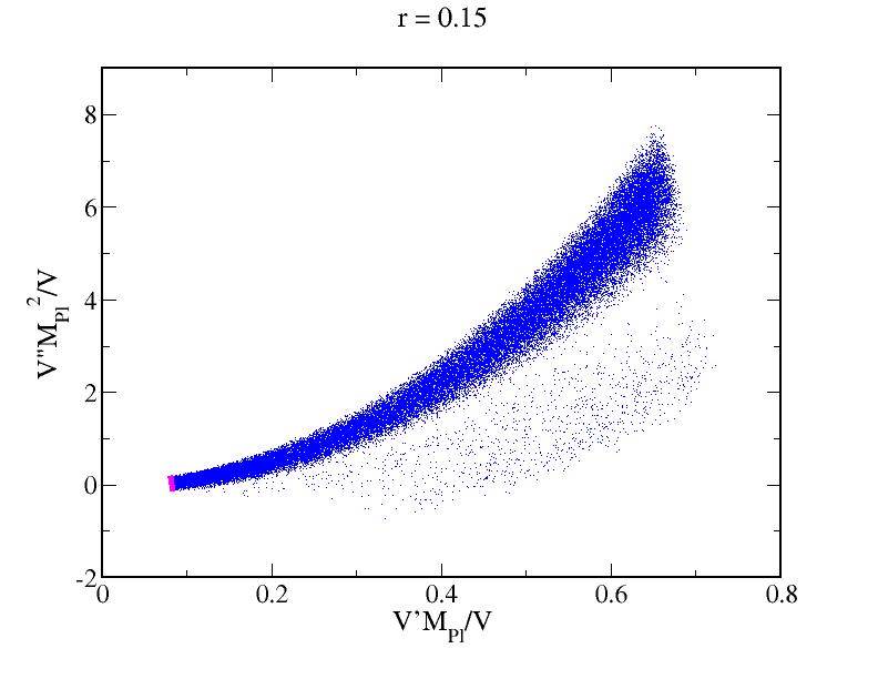
In this section we perform Monte Carlo reconstruction of DBI inflation at Planck-precision in the event that non-Gaussianities are not detected, corresponding to () (68% CL) [27]. This case was first investigated using both Bayesian and flow methods in [24]555In Ref. [24], a more optimistic detection threshold for than that considered here was used.. We consider projected constraints from Planck and CBMPol: for Planck we consider 68% CL detections of (, ) [40], (), and () [41], and for CMBPol we assume 68% CL detections of (, ), (), and () [27]. We again consider three different fiducial values for the tensor/scalar ratio: , and , and fix and . In Figure 1 we present 50,000 models each of canonical inflation (magenta) and DBI inflation (blue). There is a significant disparity between the constraints on in the case of DBI versus canonical inflation, consistent with the findings of [24]. The uncertainties in and are about a factor of 10 and 12 greater, respectively, for DBI relative to canonical inflation with fiducial . For , the uncertainties are increased by more than an order of magnitude. Similar to our findings in [4], the reconstruction achievable with Planck in the absence of tensors () is comparable to that achieved with a detection of tensors by CMBPol (with fiducial ). The fact that CMBPol fails to improve constraints on in the presence of both a curvaton and DBI degeneracy suggests that this problem is widespread amongst degenerate models. It must be stressed that a determination of still serves to reliably constrain the energy scale of inflation, even amongst models described by more general Lagrangians. And, we will see in the case of DBI inflation, as we did with curvatons in [4], that a measurement of both and will prove to be quite advantageous to the reconstruction effort [3]. However, the results in Figure 1 indicate that improvements in a measurement of on its own offer little corresponding improvement in reconstruction results.
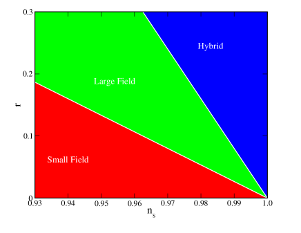
Before investigating how additional observables can improve on the degenerate case, we examine the effect of the degeneracy on the zoology classification of inflation models [42, 43]. In canonical single field inflation, models fall into distinct families with unique observable predictions in the plane. Hybrid models are generally monotonic polynomial potentials with nonvanishing vacuum energy at their minimum satisfying and . Large field models are also generally monotonic polynomials but with a true vacuum at the minimum. In order to obtain sufficient inflation with these kinds of potentials, the initial field displacement must be large in Planck units. Large field models satisfy and . Lastly, small field models are monotonic polynomials only near their local maxima – they prototypically resemble the potentials of ‘new inflation’ and those governing spontaneous symmetry breaking. They satisfy and . We present the zoology for canonical single field inflation in Figure 2 (a). At lowest order, the regions are delineated by the observable conditions,
| (3.45) | |||||
| (3.46) |
While a zoology exists for DBI inflation, the conditions that define boundaries of the observable regions depend on ,
| (3.47) | |||||
| (3.48) |
It is apparent that any uncertainty in will translate into an uncertainty in exactly where to draw these delineations – there will exist regions in which models cannot be uniquely classified according to the zoology. These regions are degenerate in that they result from the overlap of at least two classes. In the case just considered in which non-Gaussianities are not discovered in future missions, we find an uncertainty , and the resulting zoology shown in Figure 2 (b).
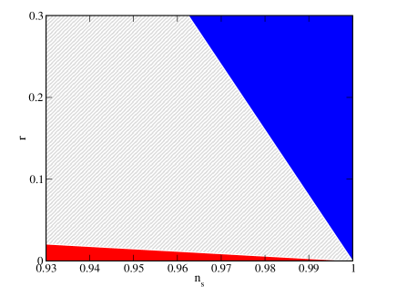
The gray region in Figure 2 (b) corresponds to a large degenerate area: hybrid DBI models overlap large field canonical models, and large field DBI models overlap a large portion of the small field canonical region.
3.4.2 Detection of Non-Gaussianity
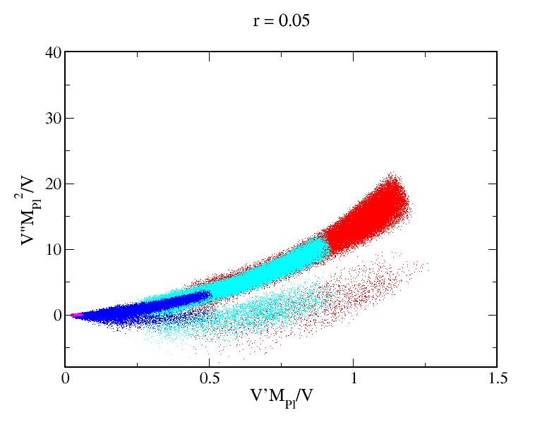
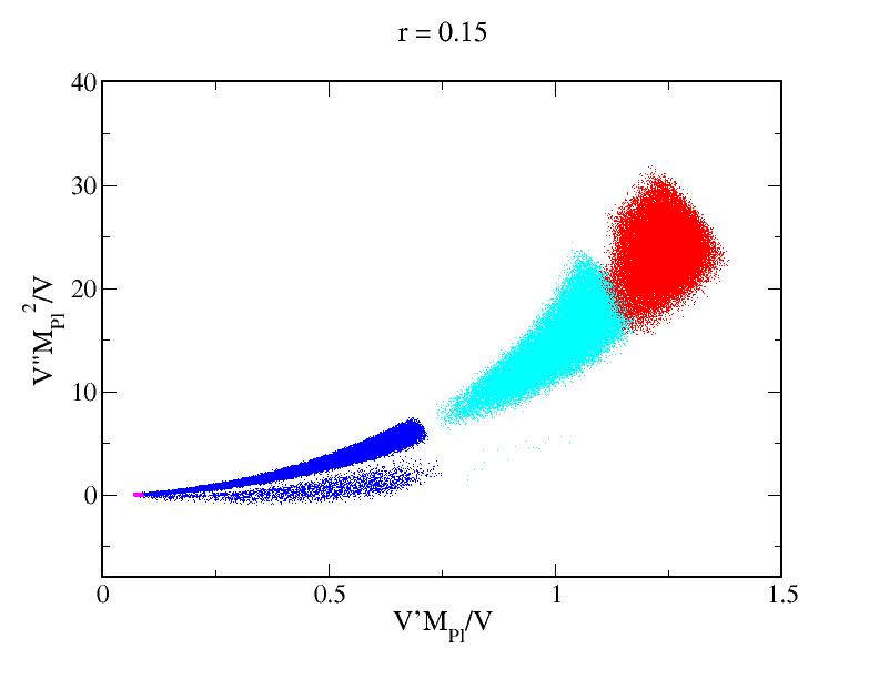
We next consider the case in which equilateral non-Gaussianities are detected in the future at Planck-precision. While such an observation breaks any degeneracy with canonical inflation, the reconstruction is still limited by the precision with which the degeneracy-breaking observables are measured. Throughout this analysis, we therefore include the reconstructed canonical models generating the equivalent and for comparison.
For each fiducial value of the tensor/scalar ratio we present results in Figure 3 for two possible observations: (cyan) and (red). We retain the models from Figure 2 for context. The Planck-sized error on translates to a 68% CL uncertainty in the -factor of for and for . As the value of increases, the resulting central values of and shift, although the shift is only greater than the individual errors in the potential parameters for moderate values of , as seen by comparing Figure 3 (a) and (b). Meanwhile, since , the error on is reduced for larger non-Gaussianities and we consequently expect the uncertainties in to be smaller as is increased, although this is only evident in Figure 3 (b) for . The unexpected increase in the error on between the non-detection of non-Gaussianities (blue) and the positive detection (cyan and red), seen particularly in Figure 3 (a), is instead a result of the fact that the we have taken the 68% limit for a null detection of non-Gaussianities to coincide with the 68% CL associated with a positive detection666While not strictly correct, in comparison with the order of magnitude disparity between the canonical and DBI reconstructions, the distinction between the 68% limit of the hypothesis test and the 68% CL of the detection is unimportant.. This, in conjunction with the constraint , results in a one-tailed distribution for the null case and a smaller error. We therefore see that in no case does a a measurement of the amplitude result in a clear improvement in both and over a null detection.
In addition to a detection of the amplitude , we also examined the effects that a measurement of the running Eq. (3.28) has on reconstruction. From Eq. (3.27), and with
| (3.49) |
where is defined as in Eq. 2, we find
| (3.50) |
We see that is unconstrained by a measurement of , and instead the higher-order parameter, , largely determines the scale dependence. This fact, coupled with the large projected errors on Eq. (3.29), results in no improvement in constraints on with over the degenerate case.
3.4.3 Direct Detection of Primordial Gravitational Waves
![[Uncaptioned image]](/html/1212.4154/assets/ndbi7.jpg)
![[Uncaptioned image]](/html/1212.4154/assets/ndbi9.jpg)
![[Uncaptioned image]](/html/1212.4154/assets/ndbi10.jpg)
![[Uncaptioned image]](/html/1212.4154/assets/ndbi11.jpg)
![[Uncaptioned image]](/html/1212.4154/assets/ndbi12.jpg)
![[Uncaptioned image]](/html/1212.4154/assets/ndbi13.jpg)
![[Uncaptioned image]](/html/1212.4154/assets/ndbi14.jpg)
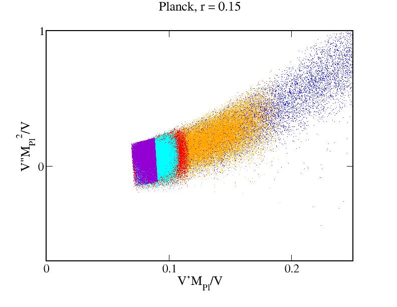
As a last case, we study the effect that a direct detection of primordial gravitational waves has on DBI reconstruction. We consider possible detections with three prospective probes: BBO-standard, BBO-grand, and DECIGO. This analysis provides additional details in support of results presented in [3]. We assume a tensor spectrum of the form
| (3.51) |
where is the tensor index running, and determine the uncertainty in the measurement of from
| (3.52) |
where and , and characterizes the experiment: , 2.5, 100 for BBO-standard, BBO-grand, and DECIGO, respectively. The amplitude of the gravitational wave signal, , is constrained on the scale of direct detection ( Mpc-1) to lie within the 68% CL, . We choose fiducial values consistent with a power law spectrum that obey the canonical single field consistency relation .
This choice of fiducial values is in agreement with both canonical and DBI inflation, and so unlike the non-Gaussianities just considered, primordial gravitational waves do not break the degeneracy in this case. However, a precision measurement of , coupled with a determination of , nonetheless enables an improved reconstruction of despite the persistent degeneracy because of the modified consistency relation, Eq. (3.30). The potential coefficients, Eqs. (3.1), become
| (3.53) | |||||
| (3.54) |
with no longer any dependency on . We present results in Figure 4 for the fiducial values: , , , , and , . We find that for , direct detection offers no improvement over the degenerate case shown in Figure 1 (d); however, improvements begin to emerge as the value of increases. With a detection of with CMBPol and with DECIGO, the DBI reconstruction becomes comparable to that of canonical inflation (Figures 4 (d),(e)). Even the less optimistic outcome of a Planck detection of tensors with and a BBO-grand measurement of , we find that the DBI potential space can be constrained to within a factor of a few of the canonical reconstruction (Figures 4 (a),(b)).
For completeness and comparison, we also consider the reconstruction that follows from the determination of from an ideal B mode measurement on CMB scales (Figures 4 (f)-(h)). We take the uncertainties in for the ideal experiment to be at , at , and at [45]. The constraints are slightly worse but competitive with those obtained with CMBPol+BBO-grand. We summarize all of our findings in Table 1.
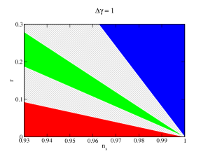
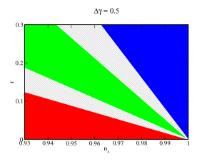
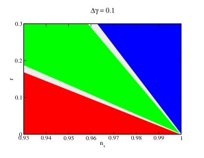
Given the improved constraints on obtainable with , we now revisit the zoology classification. Earlier, we obtained the zoology in the absence of , Figure 2 (b), and found that much of the available parameter space could not be uniquely assigned to a potential class. This was a result of the fact that was virtually unconstrained. However, with a detection of , in many cases the limits of are much improved (c.f. Table 1): for with Planck and with CMBPol and an ideal experiment. Rather than determine the zoology for each combination in Table 1, we present in Figures 5 (a)-(c) the zoology that results for , 0.5, and 0.1. The zoology is almost restored for , obtained with CMBPol+BBO-grand or DECIGO for .
| Observation | Zoology unique? | |||||
|---|---|---|---|---|---|---|
| No NG/ | 9/28 | 12/14 | 1 | 1 | 9 | H |
| NG () | 18/84 | 24/42 | 2/3 | 2/3 | 5.5 | H |
| NG () | 9/14 | 24/28 | 1/0.5 | 2/2 | 3 | H |
| NG () | 9/28 | 12/14 | 1 | 1 | 9 | H |
| (Planck + BBOs) | 9/7 | 12/2 | 1/0.25 | 1/0.0625 | 400/2 | H |
| (Planck + BBOg) | 5/2.5 | 8/1.25 | 0.5/0.08 | 0.5/0.03 | 55/0.75 | H |
| (Planck + DEC) | 3/2 | 5/1.25 | 0.25/0.05 | 0.25/0.03 | 40/0.5 | H/LF,H |
| (CMBPol + BBOs) | 30/40/15 | 11/6/2 | 1/0.6/0.2 | 1/0.25/0.0625 | 125/15/1 | H/H/H |
| (CMBPol + BBOg) | 30/8/3 | 11/1.5/1 | 1/0.1/0.03 | 1/0.08/0.03 | 125/1/0.15 | H/H/LF,H |
| (CMBPol + DEC) | 30/3/1.75 | 11/1.25/1 | 1/0.035/0.015 | 1/0.08/0.03 | 40/0.5/0.1 | H/SF,H/LF,H |
| (ideal B mode) | 30/16/7 | 11/2/1 | 1/0.2/0.1 | 1/0.1/0.05 | 125/1.75/0.5 | H,H,LF,H |
4 Discussion
In this paper we have studied the degeneracy problem in the context of non-canonical inflation, focusing on DBI inflation as a prototype. Our main goal in this endeavor has been to provide an estimate of the size of degeneracy that exists between canonically normalized single field inflationary models and DBI models in the event that no observables beyond the scalar and tensor two-point functions are measured. This ‘worst case scenario’ makes it impossible to reconstruct the inflationary potential or categorize the inflationary model according to the standard zoology scheme. This is of course only the ‘tip of the iceberg’, as many other -inflation models and (even other paradigms such as the curvaton as discussed in [4]) exacerbate the problem. We then demonstrate the ability of additional observables such as non-Gaussianity, B-mode polarization and direct detection of primordial gravitational waves to both break the degeneracy and improve the potential reconstruction program.
Our results show that even though detection of the amplitude of clearly breaks the degeneracy between models the detection does not improve reconstruction of the inflationary potential. Then we show that direct measurement of the tensor perturbation spectral index , which does not help to break degeneracy, does result in significantly improved potential reconstruction when combined with an accurate determination of the tensor-to-scalar ratio via the modified consistency relation [3]. Without the measurement of , measurements of , even at precision greater than that achievable by Planck, does not lead to an improvement in potential reconstruction. In the best case scenario, measurements of and (which serves to constrain the sound speed in DBI inflationary models) can result in an impressive restoration of the inflationary zoology.
Acknowledgments
The work of DAE is supported in part by the DOE under DE-SC0008016 and by the Cosmology Initiative at Arizona State University.
References
- [1] A. H. Guth, Phys. Rev. D 23, 347 (1981).
- [2] A. D. Linde, Phys. Lett. B 108, 389 (1982).
- [3] D. A. Easson and B. A. Powell, Phys. Rev. Lett. 106, 191302 (2011) [arXiv:1009.3741 [astro-ph.CO]].
- [4] D. A. Easson and B. A. Powell, Phys. Rev. D 83, 043502 (2011) [arXiv:1011.0434 [astro-ph.CO]].
- [5] D. A. Easson, S. Mukohyama and B. A. Powell, Phys. Rev. D 81, 023512 (2010) [arXiv:0910.1353 [astro-ph.CO]].
- [6] R. Bean, D. J. H. Chung and G. Geshnizjani, Phys. Rev. D 78, 023517 (2008) [arXiv:0801.0742 [astro-ph]].
- [7] C. Armendariz-Picon, T. Damour and V. F. Mukhanov, Phys. Lett. B 458, 209 (1999) [arXiv:hep-th/9904075].
- [8] W. Zhao and Q. -G. Huang, Class. Quant. Grav. 28, 235003 (2011) [arXiv:1101.3163 [astro-ph.CO]].
- [9] G. R. Dvali and S. H. H. Tye, Phys. Lett. B 450, 72 (1999) [arXiv:hep-ph/9812483].
- [10] S. H. S. Alexander, Phys. Rev. D 65, 023507 (2002) [arXiv:hep-th/0105032].
- [11] G. R. Dvali, Q. Shafi and S. Solganik, arXiv:hep-th/0105203.
- [12] C. P. Burgess, M. Majumdar, D. Nolte, F. Quevedo, G. Rajesh and R. J. Zhang, JHEP 0107, 047 (2001) [arXiv:hep-th/0105204].
- [13] J. H. Brodie and D. A. Easson, JCAP 0312, 004 (2003) [arXiv:hep-th/0301138].
- [14] S. Kachru, R. Kallosh, A. Linde, J. M. Maldacena, L. P. McAllister and S. P. Trivedi, JCAP 0310, 013 (2003) [arXiv:hep-th/0308055].
- [15] E. Silverstein and D. Tong, Phys. Rev. D 70, 103505 (2004) [arXiv:hep-th/0310221].
- [16] M. Alishahiha, E. Silverstein and D. Tong, Phys. Rev. D 70, 123505 (2004) [arXiv:hep-th/0404084].
- [17] A. R. Liddle, P. Parsons and J. D. Barrow, Phys. Rev. D 50, 7222 (1994) [arXiv:astro-ph/9408015].
- [18] E. Babichev, V. Mukhanov and A. Vikman, JHEP 0802, 101 (2008) [arXiv:0708.0561 [hep-th]].
- [19] S. B. Giddings, S. Kachru and J. Polchinski, Phys. Rev. D 66, 106006 (2002) [hep-th/0105097].
- [20] M. R. Douglas and S. Kachru, Rev. Mod. Phys. 79, 733 (2007) [arXiv:hep-th/0610102].
- [21] X. Chen, JHEP 0508, 045 (2005) [arXiv:hep-th/0501184].
- [22] J. Garriga and V. F. Mukhanov, Phys. Lett. B 458, 219 (1999) [arXiv:hep-th/9904176].
- [23] N. Agarwal and R. Bean, Phys. Rev. D 79, 023503 (2009) [arXiv:0809.2798 [astro-ph]].
- [24] B. A. Powell, K. Tzirakis and W. H. Kinney, JCAP 0904, 019 (2009) [arXiv:0812.1797 [astro-ph]].
- [25] X. Chen, M. x. Huang, S. Kachru and G. Shiu, JCAP 0701, 002 (2007) [arXiv:hep-th/0605045].
- [26] E. Komatsu et al. [WMAP Collaboration], Astrophys. J. Suppl. 192, 18 (2011) [arXiv:1001.4538 [astro-ph.CO]].
- [27] D. Baumann et al. [CMBPol Study Team Collaboration], AIP Conf. Proc. 1141, 10 (2009) [arXiv:0811.3919 [astro-ph]].
- [28] X. Chen, Phys. Rev. D 72, 123518 (2005) [arXiv:astro-ph/0507053].
- [29] E. Sefusatti, M. Liguori, A. P. S. Yadav, M. G. Jackson and E. Pajer, JCAP 0912, 022 (2009) [arXiv:0906.0232 [astro-ph.CO]].
- [30] See: http://universe.nasa.gov/program/bbo.html
- [31] N. Seto, S. Kawamura and T. Nakamura, Phys. Rev. Lett. 87, 221103 (2001) [arXiv:astro-ph/0108011].
- [32] N. Seto, Phys. Rev. D 73, 063001 (2006) [arXiv:gr-qc/0510067].
- [33] H. Kudoh, A. Taruya, T. Hiramatsu and Y. Himemoto, Phys. Rev. D 73, 064006 (2006) [arXiv:gr-qc/0511145].
- [34] M. B. Hoffman and M. S. Turner, Phys. Rev. D 64, 023506 (2001) [arXiv:astro-ph/0006321].
- [35] W. H. Kinney, Phys. Rev. D 66, 083508 (2002) [arXiv:astro-ph/0206032].
- [36] R. Easther and W. H. Kinney, Phys. Rev. D 67, 043511 (2003) [arXiv:astro-ph/0210345].
- [37] H. V. Peiris, D. Baumann, B. Friedman and A. Cooray, Phys. Rev. D 76, 103517 (2007) [arXiv:0706.1240 [astro-ph]].
- [38] W. H. Kinney and K. Tzirakis, Phys. Rev. D 77, 103517 (2008) [arXiv:0712.2043 [astro-ph]].
- [39] L. Lorenz, J. Martin and C. Ringeval, Phys. Rev. D 78, 083513 (2008) [arXiv:0807.3037 [astro-ph]].
- [40] L. P. L. Colombo, E. Pierpaoli and J. R. Pritchard, Mon. Not. Roy. Astron. Soc. 398, 1621 (2009) [arXiv:0811.2622 [astro-ph]].
- [41] J. R. Bond, C. R. Contaldi, A. M. Lewis and D. Pogosyan, Int. J. Theor. Phys. 43, 599 (2004) [arXiv:astro-ph/0406195].
- [42] S. Dodelson, W. H. Kinney and E. W. Kolb, Phys. Rev. D 56, 3207 (1997) [arXiv:astro-ph/9702166].
- [43] W. H. Kinney, E. W. Kolb, A. Melchiorri and A. Riotto, Phys. Rev. D 69, 103516 (2004) [arXiv:hep-ph/0305130].
- [44] W. Zhao and W. Zhang, Phys. Lett. B 677, 16 (2009) [arXiv:0907.1453 [astro-ph.CO]].
- [45] W. Zhao and D. Baskaran, Phys. Rev. D 79, 083003 (2009) [arXiv:0902.1851 [astro-ph.CO]].
- [46] J. B. Dent, D. A. Easson and H. Tashiro, Phys. Rev. D 86, 023514 (2012) [arXiv:1202.6066 [astro-ph.CO]].
- [47] A. Cooray, Phys. Rev. Lett. 97, 261301 (2006) [astro-ph/0610257].
- [48] P. Adshead, R. Easther, J. Pritchard and A. Loeb, JCAP 1102, 021 (2011) [arXiv:1007.3748 [astro-ph.CO]].