Properties of ultra-cool dwarfs with Gaia

Abstract

Context. The Gaia catalogue will contain observations and physical parameters of a vast number of objects, including ultra-cool dwarf stars, which we define here as stars with a temperature below 2500 K.

Aims. We aimed to assess the accuracy of the Gaia $T_{\rm eff}$ and $\log(g)$ estimates as derived with current models and observations.

Methods. We assessed the validity of several inference techniques for deriving the physical parameters of ultra-cool dwarf stars: Gaussian processes, support vector machines, $k$-nearest neighbours, kernel partial least squares and Bayesian estimation. In addition, we tested the potential benefits of data compression for improving robustness and speed. We used synthetic spectra derived from ultra-cool dwarf models to construct (train) the regression models. We derived the intrinsic uncertainties of the best inference models and assessed their validity by comparing the estimated parameters with the values derived in the bibliography for a sample of ultra-cool dwarf stars observed from the ground.

Results. We estimated the total number of ultra-cool dwarfs per spectral subtype, and obtained values that can be summarised (in orders of magnitude) as 400000 objects in the M5-L0 range, 600 objects between L0 and L5, 30 objects between L5 and T0, and 10 objects between T0 and T8. A bright ultra-cool dwarf (with $T_{\rm eff}$=2500 K and $\log(g)$=3.5) will be detected by Gaia out to approximately 220 pc, while for $T_{\rm eff}$=1500 K (spectral type L5) and the same surface gravity, this maximum distance reduces to 10-20 pc. We found the cross-validation RMSE prediction error to be 10 K for regression models based on the $k$-nearest neighbours and 62 K for Gaussian process models in the faintest limit (Gaia magnitude G=20). However these values correspond to the evaluation of the regression models with independent test sets of synthetic spectra of the same model families as used in the training phase (internal errors). For the $k$-nearest neighbours model, this seems an overly optimistic error estimate due to the use of a dense grid of examples in the training set, together with a relatively high signal-to-noise ratio for the end-of-mission data. The RMSE of the prediction deduced from ground-based spectra of ultra-cool dwarfs simulated at the Gaia spectral range and resolution, and for a Gaia magnitude G=20 is 213 K and 266 K for the models based on $k$-nearest neighbours and Gaussian process regression, respectively. These are total errors in the sense that they include the internal and external errors, with the latter caused by the inability of the synthetic spectral models (used for the construction of the regression models) to exactly reproduce the observed spectra, and by the large uncertainties in the current calibrations of spectral types and effective temperatures. We found maximum-likelihood methods (minimum $\chi^{2}$, $k$-nearest neighbours, and Bayesian estimation with flat priors) to be biased in the L0-T0 range in that they systematically assign a temperature around 1700 K. Finally, the likelihood landscape is significantly multimodal in spectra with realistic noise.

1 Introduction

In this work we define an ultra-cool star as a star with an effective temperature below 2500 K (spectral type M8). The goal of this paper is to assess the detectability of this type of object with the Gaia spacecraft. Gaia is a mission of the European Space Agency that will produce very accurate astrometry and parallaxes for a significant fraction of the galactic population (de Bruijne 2012), thus helping to considerably improve our knowledge of a plethora of astronomical topics, from stellar evolution to exoplanets. In particular, Gaia data will improve our understanding of the nature of ultra-cool dwarfs by providing distances and therefore luminosities for the nearest objects. The 2MASS All-Sky survey (Cutri et al. 1996) began a new era in the discovery and characterisation of very-late spectral type stars and brown dwarfs, allowing the identification of two new types: L (Kirpatrick et al. 1999; Martín et al. 1997) and T (Kirpatrick et al. 1999; Burgasser et al. 2002), and paving the way for even cooler objects, the Y type (Burningham et al. 2008; Kirkpatrick et al. 2012). Subsequent surveys have discovered hundreds of cool objects, but the comprehensive understanding of their nature relies in modelling from internal structure to atmospheres. This can only be achieved with precise data, including accurate distances. Here, Gaia will truly play the role of a Rosetta stone.

The work presented here was developed in the framework of the eighth coordination unit (CU8) of the Gaia Data Processing and Analysis Consortium (DPAC), which is devoted to determining astrophysical parameters. Gaia is expected to detect and characterise one billion sources, and hence, automatic procedures for the reduction and processing of these data are essential.

The DPAC consortium is, in charge of the design, development, and operation of this data processing and analysis chain aimed of producing the Gaia catalogue (intermediate releases and final catalogue) from the telemetry data (see Mignard et al. (2008) for a more detailed introduction to the DPAC).

Since potential Gaia targets include very different astrophysical scenarios, from unresolved galaxies and quasars to asteroids, specialised modules have been designed and implemented within the DPAC to characterise the various object types.

The astrophysical parameters in CU8 are determined by various modules integrated in the the Apsis pipeline. Apsis includes an initial classification into broad object categories (Bailer-Jones et al. 2008), modules for derivating stellar parameters from (amongst other observables) very low- and medium-resolution spectra (Liu et al. 2012; Recio-Blanco et al. 2006, respectively), and specialised modules for characterising of unresolved galaxies (Tsalmantza et al. 2012), quasars, or peculiar types of stars such as emission-line stars (Blomme et al. 2011), or cool stars.

In particular, a specific module of the Gaia processing pipeline is devoted to characterising ultra-cool dwarfs (hereafter UCDs), which constitutes a regression problem in which the source parameters are estimated from observational data. In the next section, we describe this module and estimate the number of sources that will be detected as a function of spectral type. In Sect. 3 we briefly describe the statistical techniques explored in the search for an optimum model for the regression problem of determining the source parameters, together with the experiments carried out in order to select amongst them. In Sect. 4 we describe the results obtained by these models when they are applied to simulated Gaia spectra of well-known ultra-cool dwarfs observed with ground telescopes. These results provide a pre-launch approximation to the expected accuracy of the Gaia parameter estimates (mainly for the effective temperature). Finally, Sect. 5 summarises the main results of this work and describes the experiments that are currently being carried out to complete this study.

2 Gaia sample of ultra-cool dwarfs

2.1 Brief description of the Gaia capabilities

The Gaia astrometric mission was approved by the European Space Agency in 2000 and the construction of the spacecraft and payload is on-going for a launch in mid 2013. Gaia will continuously scan the entire sky for five years, yielding positional and velocity measurements with the accuracies needed to produce a stereoscopic and kinematic census of about one billion stars throughout our Galaxy and beyond. The stellar survey will be complete to Gaia magnitude $G=20$ mag, with a precision of 24 $\mu$as at magnitude V=15 for a solar-type star (G2V). Gaia will be equipped with two spectrophotometers operating in the 330-680 nm range (blue photometer or BP) and in the 640-1000 nm range (red photometer or RP). Both spectrophotometers are based on a dispersive-prism approach, and the spectral resolutions are, in both cases, wavelength dependent. The RP has a varying resolution from 7 nm pixel^-1 at 640 nm to 15 nm pixel^-1 at 1000 nm, while the BP photometer resolution reaches from 4 to 32 nm pixel^-1 in its wavelength range. The details of the Gaia passband G and the photometric performances of the Gaia instruments are summarised in Jordi et al. (2010).

2.2 Ultra-cool dwarfs with Gaia

The spectral energy distributions (SEDs) of ultra-cool dwarfs all peak in the infrared range, and we do not expect any significant flux in the BP range (see Fig. 1). Therefore, we will mainly be concerned with detecting and characterising of these stars using RP spectra.

Figure 1: Normalised sample spectra from the BT-Settl library. The top row shows simulated Gaia RP spectra of BT-Settl models for $T_{\rm eff}$ = 500, 1000, 1500, 2000, and 2500 K. The vertical axis is proportional to the number of photons detected in each wavelength bin. The line colours reflect the various values of $\log(g)$ available in the library of models according to the colour scale on the right. The bottom row shows the original spectra with the same temperatures as in the top row, $\log(g)=5.0$ and solar metallicity.

A rough estimate of the number of ultra-cool dwarfs that will be detected by Gaia per bin of spectral type can be obtained asuming a local volume density such as the one compiled by Caballero et al. (2008). These authors compiled (or derived) local densities of late-type stars and brown dwarfs between spectral types M3 and T8 from the literature, to provide estimates of contamination rates by these objecs in deep photometric surveys that searched for substellar objects or high-redshift quasars. The overall shape of the local density as a function of spectral type shows three local maxima at M3, L5, and T8, and reaches a minimum of 0.22$\times 10^{-3}$ objects per cubic parsec at spectral types T0-T1. For each spectral type, we computed the distance at which a main-sequence object of the corresponding I-band absolute magnitude would reach the Gaia detection limit of G=20 using the Gaia object generator. This (hereafter GOG) is one of the three Gaia generators of simulated data that also include GASS (telemetry generator) and GIBIS (image generator). The GOG is a tool designed to obtain directly simulated catalogue and main database data for the Gaia satellite, passing through the entire mission data reduction chain (Robin et al. 2012). The outputs are astrometric, photometric, and spectroscopic epoch and final data. To simulate the main database data lifecycle, GOG uses error models whose formulas are coded using the current knowledge of the Gaia mission performances. In this work, we used GOG simulations of two synthetic libraries of ultra-cool dwarf spectra to derive the maximum distance at which an ultra-cool dwarf can be detected as a function of the I-band absolute magnitude, and other properties of the Gaia UCD sample.

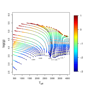
The first library is a composite of the AMES-Cond and AMES-Dusty models described in Allard et al. (2001). The validity ranges for these models are $T_{\rm eff}$ $<$ 1400 K (AMES-Cond) and $T_{\rm eff}$ $>$ 1700 K (AMES-Dusty). Therefore, there is a gap in the validity (not in the coverage) in effective temperature between 1400 and 1700 models. Models in the interregnum are available in both model families (and hence, no gap in coverage exists), and will be used in this work to interpolate between the validity domains. The second library is the BT-Settl family of models (Allard et al. 2012), valid across the entire range of effective temperatures. Figure 2 shows the evolutionary tracks for the BT-Settl library in the $T_{\rm eff}$-$\log(g)$  space for a range of masses between 0.0005 and 1.4 M_⊙. Throughout this work we measure effective temperatures in Kelvin and gravities in cm s^-2. The simulation of the synthetic spectra is carried out in practice by the so-called coordination unit 2 (CU2) of the Gaia DPAC. In most of this work we concentrated the results obtained with the BT-Settl library of models which produced better fits to the observed spectra used for validation in Sect. 4.

Figure 2: Evolutionary tracks in the $T_{\rm eff}$-$\log(g)$ space for ultra-cool dwarfs according to the BT-Settl library. Each line corresponds to a different mass in the range 0.0005–1.4M_⊙ as labelled below selected tracks. Filled circles represent individual models in the grid. These are coloured according to the decimal logarithm of the age in Gigayears as indicated by the colour scale on the right. Effective temperatures are measured in Kelvin and gravities in cm s^-2.

These two model libraries will also be used to define the mapping between the source parameters and Gaia observations described in section 3. Figure 1 shows a sample of spectra from the BT-Settl library together with the simulated Gaia RP spectra for a range of temperatures between 500 K and 2500 K. We obtained Gaia simulated data using the GOG. In the simulation of the libraries, CU2 takes into account the evolutionary tracks provided with the models.

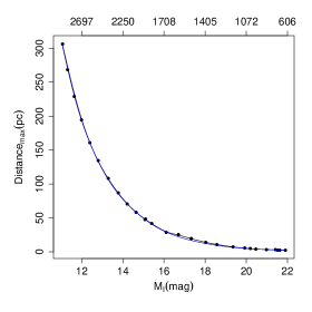
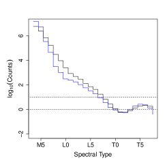
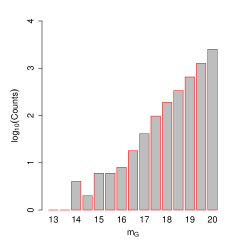
Figure 3 shows the maximum distances to main-sequence UCDs as a function of their I-band absolute magnitude. The expected number of detectable main-sequence objects in each spectral type bin can be estimated multiplying a volume density estimate (in our case, the one in Caballero et al. 2008, for spectral types between M3 and T8) by the volume of a sphere with a radius equal to the maximum distance at which an UCD corresponding to the spectral type under consideration can be detected (assuming solar metallicity). In computing these expected number counts per spectral type bin, we need to define a relationship between absolute I-band magnitude and spectral type. We used two such relations. The first one is included in Table 3 of Caballero et al. (2008) (and reproduced in Table 1 for convenience). The second relationship is derived from the I-band magnitudes and effective temperatures of the BT-Settl model family, combined with the calibration of effective temperatures with spectral types by Stephens et al. (2009). We used the analytic formula based on optical spectral types of L dwarfs and infrared spectral types of the T dwarfs. This calibration (hereafter refered to as SLC calibration) is valid in the M6 to T8 range. This analysis results in the values listed in Table 1 and illustrated in Fig. 4. Table 1 lists the relationship between spectral type and absolute magnitude in the I-band given in Caballero et al. (2008) in column 2 for reference. This results in the estimated number of counts under the column header $Counts_{CBK08}$. The relationship between spectral type and absolute magnitude in the I-band implicit to the BT-Settl model family is included in column 3. This results in the estimated number of counts under the column header $Counts_{BT-Settl}$. The SLC spectral type–effective temperature calibration (see Sect. 4) is included in column 6, and the (G_BP-G_RP) colour index computed from the noiseless GOG simulations of BT-Settl model atmospheres is included in column 7. Since the volume densities tabulated in Caballero et al. (2008) refer only to the main sequence, these estimates do not take into account the potential detection of low-gravity objects (i.e., essentially very young objects). The final increase in the expected number of counts is due to the steep increase in the volume density for spectral types later than T0. In deriving these estimates we only used BT-Settl models of solar metallicity. The expected number of detections per apparent G magnitude is shown in Fig. 4.

Figure 3: Maximum distances at which an ultra-cool dwarf can be detected by Gaia at the limiting magnitud G=20 as a function of its absolute magnitude in the I band. These have been derived from BT-Settl models (filled circles) and the continuous lines represent the interpolation used in deriving the expected counts per spectral type bin in Table 1. The black continuous line corresponds to $\log(g)$=5.0 and the blue line to $\log(g)$=3.5. The top axis shows the effective temperature measured in Kelvin for a $\log(g)$=5.0 object with the absolute I magnitudes shown in the $x$ axis, according to the BT-Settl models. The $T_{\rm eff}$–M_I mapping is only bi-valued below 600 K.

Table 1: Predicted number of counts assuming solar metallicy and auxiliary relations.

spectral type	$M_{\rm I,CBK08}$	$M_{\rm I,BT-Settl}$	$Counts_{\rm CBK08}$	$Counts_{\rm BT-Settl}$	$T_{\rm eff}$	(GBP-GRP)
M3–4 V	9.07	10.24	$1.6\times 10^{7}$	$5.7\times 10^{6}$	3269	2.86
M4–5 V	10.14	10.86	$5.4\times 10^{6}$	$2.4\times 10^{6}$	3065	3.33
M5–6 V	11.91	11.39	$3.4\times 10^{5}$	$7.0\times 10^{5}$	2889	3.74
M6–7 V	12.90	11.92	$4.3\times 10^{4}$	$1.7\times 10^{5}$	2731	4.10
M7–8 V	14.16	12.47	$3.0\times 10^{3}$	$3.0\times 10^{4}$	2583	4.44
M8–9 V	14.68	13.05	$1.0\times 10^{3}$	$9.4\times 10^{3}$	2441	4.77
M9–L0 V	15.23	13.66	$3.0\times 10^{2}$	$2.5\times 10^{3}$	2303	5.03
L0–1 V	15.27	14.30	$2.3\times 10^{2}$	$8.4\times 10^{2}$	2166	5.07
L1–2 V	15.69	14.95	$1.7\times 10^{2}$	$4.9\times 10^{2}$	2032	5.10
L2–3 V	16.19	15.44	$1.0\times 10^{2}$	$2.9\times 10^{2}$	1902	5.62
L3–4 V	16.67	15.87	$5.4\times 10^{1}$	$1.3\times 10^{2}$	1777	5.35
L4–5 V	17.14	16.38	$3.2\times 10^{1}$	$7.2\times 10^{1}$	1660	5.15
L5–6 V	17.61	16.97	$1.8\times 10^{1}$	$4.3\times 10^{1}$	1554	8.02
L6–7 V	18.07	17.57	$8.7$	$1.8\times 10^{1}$	1460	9.05
L7–8 V	18.52	18.09	$3.7$	$6.8$	1381	9.85
L8–9 V	18.90	18.49	$1.5$	$2.7$	1318	10.38
L9–T0 V	18.95	18.78	$9.4\times 10^{-1}$	$1.1$	1270	10.81
T0–1 V	19.01	18.97	$6.1\times 10^{-1}$	$6.1\times 10^{-1}$	1237	11.17
T1–2 V	19.04	19.10	$6.4\times 10^{-1}$	$5.5\times 10^{-1}$	1214	11.44
T2–3 V	19.04	19.19	$1.1$	$8.0\times 10^{-1}$	1196	11.64
T3–4 V	19.07	19.29	$2.0$	$1.3$	1176	11.84
T4–5 V	19.22	19.44	$2.9$	$1.9$	1144	12.15
T5–6 V	19.61	19.68	$2.6$	$2.1$	1086	12.61
T6–7 V	20.35	20.05	$1.2$	$1.8$	986	12.99
T7–8 V	21.60	20.62	$4.0\times 10^{-1}$	$1.4$	824	12.46

Figure 4: Predicted number of counts per spectral type bin (a) and per apparent G magnitude (b), in logarithmic units. The black line in the left panel corresponds to the derivation based on the relation between spectral type and I-band absolute magnitude included in Caballero et al. (2008), while the blue continuous line corresponds to the relation derived from the BT-Settl model family and the SLC calibration. The two horizontal (dashed) lines indicate the levels of predicted counts equal to one and ten. The right-hand side plot has been obtained assuming the relation between effective temperature and I-band absolute magnitude derived from the BT-Settl models and the SLC calibration.

2.3 Selection criteria and contamination rates

In the Gaia processing pipeline a source will only be characterised as an ultra-cool dwarf if the following conditions are met:

1. Its estimated distance is smaller than the maximum distance at which an ultra-cool star can be detected. This is the distance at which the brightest ultra-cool star would have a Gaia limiting magnitude of G=20. We estimated the maximum brightness of an ultra-cool star from the BT-Settl models, and it corresponds to the hottest model with the lowest surface gravity.

2. The source is fainter (in the G band) than the brightests model placed at the same distance as estimated by Gaia.

3. The BP-RP colour index is higher (redder) than the minimum (bluest) colour index found in the model libraries.

4. The celestial coordinates and proper motions are not consistent with solar system Keplerian motions.

Sources that fulfil these criteria (within some margin that depends on the measurement uncertainties) are subsequently processed to estimate their effective temperature and surface gravity as described in section 3. Objects not detected in the BP band (but fulfilling all other criteria) will nevertheless be selected because the non-detection is itself an indication of a red spectrum. This could imply a potential contamination of the UCD sample by faint, nearby objects close to the Gaia limiting magnitude and colour indices that are positive (thus excluding white dwarfs), but bluer than the bluest UCD. The software that implements the analysis of ultra-cool dwarfs distinguishes between the selection module that decides whether to process a given Gaia source, and the processing module that estimates the effective temperature and gravity of the selected sources.

To define the boundaries of brightness, colour index, and distance that define the region of ultra-cool sources, we analysed the GOG simulations of the AMES-Cond, AMES-Dusty and BT-Settl model libraries (although the latter is prefered, and the former have not been implemented in the selection software). Using GOG, we found that the most distant ultra-cool object in the library (a source with $T_{\rm eff}$ = 2500 K and $\log(g)$ = 3.5 at G=20) corresponds to a distance of 373 pc. Thus, the first criterion limits the processing of sources by the UCD module to sources within this radius (this is necessary optimise the processing time per source). The second criterion examines the brightness of each detected source and compares it with the aforementioned brightest model placed at the same distance. We expect a strong contamination from main-sequence stars with temperatures above the 2500 K limit because low-gravity sources are brighter than main-sequence ones for temperatures above 1600 K. In fact, we derived from the GOG simulation of the model libraries that a dwarf star of $\approx 4180$ K has the same G magnitude as the lowest gravity, hottest ultra-cool giant considered in this work ($T_{\rm eff}$ = 2500 K, $\log(g)$ = 3.5). Thus, main-sequence objects up to this temperature will be selected by the selection module according to this criterium despite their higher temperatures (although the colour index criterium will reject a fraction of these hotter stars; see below). We could have used the thresholds corresponding to the main-sequence objects, but this would have resulted in the potential loss of low-gravity sources in the selection process. We opted for an inclusive set of criteria in spite of the expected high contamination rates by dwarfs hotter than 2500 K. To estimate the contamination rate (caused by the criteria but also to the measurement errors), we conducted a numerical experiment in which we populated a one-kiloparsec cube with sources uniformly distributed in space (this is much larger than actually needed in view of the estimated maximum distance to an UCD). The total number of sources in each temperature bin was generated using a probability density function derived by interpolating and normalising the volume densitites tabulated in Caballero et al. (2008). Since these correspond to main-sequence sources, we neglected the contribution from ultra-cool giants in the following estimates.

For each star, and given the effective temperature and the distance to the centre of the cube, we computed the apparent G magnitude and the (V-I) colour index by interpolating in the BT-Settl library restricted to dwarfs with values of $\log(g)$ $\approx$ 5.5. We subsequently used the current estimates of the uncertainties in the Gaia magnitudes and parallaxes (see Jordi et al. (2010) and de Bruijne (2009) respectively) to generate mock measurements of the distances and G magnitudes by sampling from normal distributions with the prescribed uncertainties. We did not use a full covariance matrix since none was available at the time of writing. We show in Fig. 5 the error models that we used in the simulations. The uncertainty estimate in the G magnitude is based on Eq. 6 in Jordi et al. (2010) and on the mission parameters available at the time of writing. We included a calibration error $\sigma_{cal}=$30 mmag for a single transit. This value is only an educated guess since the final $\sigma_{cal}$ can only be estimated during the operational phase. The uncertainty in the parallax is based on Eq. 1 in de Bruijne (2009) (see de Bruijne (2012) for a more recent review without analytic expressions for the astrometric uncertainty).

Figure 5: Current estimates of the end-of-mission uncertainties in the measurements of the G apparent magnitude (black line) and the parallax (dashed and dotted lines) as a function of the G apparent magnitude. The dashed line corresponds to (V-I) = 4 and the dotted line to (V-I) = 7.5, a plausible range for the V-I colour index according to the model libraries.

The resulting sample of stars in the kiloparsec cube was then examined to determine the properties of the subsample that fulfilled the criteria enumerated above (except for the non-Keplerian motion). We found that none of the ultra-cool dwarfs thus generated is missed in the selection process due to errors in the measurements. This was expected given i) the inclusiveness of the criteria, ii) the relative proximity of these faint sources to the Sun, and iii) the fact that we only generated main-sequence objects in the simulation (and not low-gravity young sources that would be closer to the selection thresholds; this question will be re-examined during the software validation phase with real Gaia data and may result in more inclusive thresholds if we identify examples of this kind missed by the selection module). The uncertainties in the G magnitude and colour index typical of UCDs according to the simulations are negligible in this context.

The (G_BP-G_RP) colour index thresholds in the selection criteria are defined by the bluest model in the GOG simulations of the model libraries. For the BT-Settl library of models and metallicities [M/H] between -2 and 0.5, we find that the (G_BP-G_RP) colour index is in the 4.1–14.5 range. The distribution of effective temperatures in the resulting sample of non-UCD stars that fulfil the criteria is shown in Fig. 6. The shape is determined by the combination of the various selection criteria and the uncertainties in the measurements.

Figure 6: Histogram of the temperatures of non-UCD stars that pass the selection criteria of the Gaia UCD module.

Fig. 6 implies a contamination rate of abound 85%. This is explained by the exponential increase in volume densities for the mid- to late-M spectral types. To take this high contamination rate into account, we generated regression models in Sect. 3 that are capable of predicting effective temperatures up to 4000 K, and not only in the UCD regime below 2500 K. Therefore, even if the selection module selects these contaminants, the processing module will allow for the obtention of purer samples of UCDs by filtering out objects with estimated temperatures above a given threshold.

In computing the contamination rate we did not consider extra-galactic contaminants because their parallax measurements would be incompatible with the selection criteria defined above.

3 Methodology

As mentioned in Sect. 1, Gaia is expected to detect and process a number of sources close to one billion. This order of magnitude necessitates automating the detection and characterization processes. The main objective of the eighth coordination unit of the Gaia DPAC is to implement and evaluate automated procedures to derive the astrophysical parameters of the sources detected by the Gaia instruments. This necessarily involves techniques developed in the fields of statistical learning and data mining. In the framework of statistical learning methods, this is accomplished with regression models that are constructed from sets of examples (the so-called training set) that link the independent variables (the Gaia observations in our case) with the dependent variables that we wish to infer. In this section we describe several techniques taken from the field of statistical learning, aimed at providing a reproducible, systematic characterization of the Gaia UCD candidate sources.

In collecting the aforementioned sets of examples, libraries of stellar models and associated synthetic spectra provide a homogeneous and consistent set of examples that uniformly cover the parameter spaces under consideration. In contrast, catalogues of observed spectra with associated astrophysical parameters derived from them tend to be fragmentary in nature: each collection covers only a reduced range of parameters, and it is necessary to combine several catalogues to obtain a coverage that, even then, may contain gaps and/or insufficiently sampled regions (this is especially true for the parameter $\log(g)$, which is missing from most compilations). Each catalogue has its own observational setup, systematic errors, and selection effects. Also, observational biases may favour the abundance of examples in particular regions of the parameter space, which then translate into systematic biases in the predictions. Furthermore, parameter estimation across catalogues can be inconsistent, and we indeed find slightly different spectral types assigned to the same source in different catalogues, which reveals a certain degree of subjectivity in the assignements. With all these considerations in mind (reproducibility, consistency, homogeneity, and uniformity of the training set), we prefered to construct our regression models from the aforementioned synthetic libraries. These libraries parameterise the models with physical magnitudes (effective temperatures, gravities, and metallicities) and not with spectral types.

Model libraries are nevertheless imperfect in the sense that they do not reproduce each and every spectral feature in the real spectra of UCDs or its exact dependence on the physical parameters. The problem of the potential mismatch between stellar model libraries and observations appears whenever physical parameters are to be produced, beyond phenomenological descriptions such as spectral types. Spectral types can be inferred without the need for synthetic models, while going from spectra (or spectral types) to physical parameters requires model libraries to interpret them. In this work we do not attempt to build regression models to infer spectral types. Given the low spectral resolution of the Gaia red spectrophotometer (RP), and its spectral coverage, most of the spectral features used to decide the spectral type remain unresolved or unobserved, and thus, spectral types derived from them would be of limited use.

The systematic effects of the selection of model libraries can be characterised to some extent by comparing the predictions from different model families like those presented in the previous section (AMES-Cond, AMES-Dusty, and BT-settl). In Sect. 4 we also attempt to validate our models with an external set of effective temperatures derived from ground-based observations and spectral types via a calibration that, inevitably, encompasses another synthetic stellar library. The two families of models introduced in the previous section (AMES-Cond and -Dusty, and the BT-Settl models) are used to define the relationship between Gaia observables (the RP spectrum) and the parameters that we intend to estimate, namely $T_{\rm eff}$ and $\log(g)$. This relationship is captured in a regression model (not to be mistaken for the physical models of the stellar atmospheres and the resulting synthetic spectra) constructed from the set of examples defined by the two synthetic spectral libraries. Each spectrum in the libraries (e.g. those represented in the lower row of Fig. 1) is characterised by the set of physical parameters that identifies the stellar atmosphere used to synthesize it. This set of examples composed of the spectrum plus the corresponding physical parameters is referred to in the following as the training set. The set of independent examples used to assess the accuracy of the models will be referred to as the test set.

As mentioned before, the training set is constructed using the AMES-Cond, -Dusty, and BT-Settl model libraries (restricted to effective temperatures below 4000 K)) and simulating Gaia observations of these synthetic models using GOG (version 8.0). Gaia has a nominal duration of five years. During this period, a source is observed on average approximately 70 times. Each time a source is observed (i.e., each transit), an epoch RP spectrum is obtained. The characteristics of this spectrum depend on the instrument design including prism and CCDs, and the transit geometric properties. In general, we can assume that the spectrum will be spread along 60 spectral bands with a non-uniform dispersion. In each transit, the position of the source (continuous) spectrum may vary with respect to the discrete CCD pixel array depending on the transit geometric details. This transit dependence results in different spectra obtained for each epoch, because the wavelength coverage of each pixel is different. This subresolution information can then be used to produce oversampled combined spectra. In Fig. 1 and in the experiments carried out in this work that are described in the following sections we assumed an end-of-mission oversampling factor of three, resulting in a total number of flux bins of 180.

3.1 Regression models

In this section we describe three different types of statistical regression models: $k$-nearest neighbours (Cover & Hart 1967), Gaussian processes (see e.g. Bishop 2006; Rasmussen & Williams 2006), and Bayesian inference (see e.g. Sivia & Skilling 2006). A previous analysis also included support vector machines (Vapnik 1995; Cortes & Vapnik 1995) and kernel partial least squares (KPLS, Rosipal et al. 2001).

$k-$nearest neighbours estimation (kNN) is by far the simplest model and derives the parameter values as the weighted average of the elements in the training set that are closest to the input spectrum in a given metric. In our case, the euclidean distance is used to define proximity and the weights are defined as the inverse of this distance. A maximum-likelihood estimate of the uncertainties in the estimated parameters can be computed by modelling the distribution of inverse distances to the nearest neighbours (under the assumptions that the model grid is sufficiently dense and the neighbourhood has the appropriate size to sample a unimodal likelihood). It has the disadvantage that the full training set has to be stored and accessed each time that the regression model is used to predict the physical parameters ($T_{\rm eff}$ and $\log(g)$) of a source, and furthermore, it is severely affected by the so-called curse of dimensionality. This is reflected in the need for exponentially growing training set sizes as the problem input dimensionality increases. The exponential growth is required to ensure that the nearest neighbours are sufficiently close to provide an accurate estimate of the parameters.

Support vector machines (SVMs) and Gaussian processess (GPs) are two examples of kernel methods. These methods transform the regression problem into a dual representation where the constituents of the model are no longer the input features (or nonlinear mappings thereof) but their scalar products expressed as kernel functions. More details of this dual representation can be found in the textbooks by Bishop (2006) and Hastie et al. (2001).

A GP is defined as a probability distribution over functions such that the joint probability of the random variables defined by their evaluations at a certain set of input vectors (the training set in our case) is Gaussian. If we assume that the nature of our problem is such that the probabilistic distribution for both the targets of our training set and the Gaia observations to be characterised is well captured by a multivariate Gaussian distribution, we can construct the model by computing its covariance matrix. It turns out that we can calculate it by evaluating the kernel functions at the input vectors of the training set. These kernel functions encode both the assumed error model for our determination of the target values in the training set and the length scale for the correlations between the examples in the training set. In the full Bayesian treatment these two parameters can be considered hyperparameters and are marginalised out. Here we have determined optimal values for them through exhaustive cross-validation experiments (see below). For the SVM, the model representation is sparse in the sense that it only depends on kernel evaluations on a small subset of the training set (the support vectors). In regression problems, the support vectors are those that lie within the boundaries of, or outside a so-called insensitive tube. Support vector regression involves the search for best (minimum error) solution in a space of hyperparameters, similar in nature to those discussed for GPs.

In this section we describe a parallel aproach to parameter estimation based on Bayes’ theorem. The main advantage of Bayesian parameter estimation stems from the fact that it provides not only an estimate of the parameters but also a full multivariate probability density distribution for the set of parameters given the observations.

We assume that we observe the spectrum $\mathbf{s}$ of an ultra-cool dwarf. In the Bayesian framework, we seek the probability density function (PDF) of the physical parameters of the UCD, given this spectrum $\mathbf{s}$. Bayes’ theorem provides this PDF as

$$\pi(\bm{\theta}|\mathbf{s})=\frac{\pi(\bm{\theta})\cdot f_{\bm{\theta}}(\mathbf{s})}{m(\mathbf{s})},$$ (1)

where $\bm{\theta}=(T_{\rm eff},\log(g))$ is the vector of parameters that we intend to derive, $\pi(\bm{\theta})$ is the prior probability distribution of these parameters, and $f_{\bm{\theta}}(\mathbf{s})$ is the likelihood of the spectrum given the parameters.

The denominator in the right-hand side of Eq. 1 $m(\mathbf{s})$ is the prior predictive distribution or evidence defined as

$$m(\mathbf{s})=\int f_{\bm{\theta}}(\mathbf{s})\,\pi(\bm{\theta})\,d\bm{\theta},$$ (2)

and can be viewed as a normalisation constant.

The likelihood term encompasses a predictive model for the spectra given the parameters, together with a probabilistic error model. In our case, we used the two stellar libraries mentioned above (COND+DUSTY and BT-Settl) to build the predictive model. This is captured in two three-layer perceptrons (a kind of neural network) each trained with the stellar spectra of the corresponding library. The neural network captures a multivariate regression model that can be used to perform an interpolation. Extensive experiments to derive the optimal network architecture result in hidden layers of 20 hidden units for the two model libraries. With it, we can generate output synthetic spectra for any input value of $\bm{\theta}$ within the grid boundaries. The neural network exactly predicts the spectra in the COND+DUSTY and BT-Settl grids, and smoothly interpolates for intermediate values. The unique flux predicted by the neural network for each wavelength in the spectrum can be turned into a probabilistic statement by convolving it with the predicted measurement errors in the current Gaia model. At present, the error model for the RP spectra consists of a Gaussian distribution with a covariance $\Sigma$ that depends on a series of instrument parameters, on the number of transits, and on the flux itself (see Jordi et al. (2010), discussed above). Thus,

$$f_{\bm{\theta}}(\mathbf{s})=f_{(\mathbf{x_{\theta}},\Sigma)}(\mathbf{s}),$$ (3)

with $\mathbf{x_{\theta}}$ being the prediction from the neural network for the parameter set $\theta$, and $f_{(\mathbf{x_{\theta}},\Sigma)}(\mathbf{s})$, the probability density function of a normal distribution $\mathcal{N}(\mathbf{x_{\theta}},\Sigma)$ evaluated at the observed spectrum $\mathbf{s}$.

Nested sampling (Skilling 2006) is a Monte Carlo procedure used to calculate $m(\mathbf{s})$ that can extract samples from $\pi(\bm{\theta}|\mathbf{s})$ as a by-product of these calculations. The algorithm exploits the relation between the likelihood $f_{\bm{\theta}}(\mathbf{s})$ and the prior volume $X$ defined by

$$X(\lambda)=\int_{f_{\bm{\theta}}(\mathbf{s})>\lambda}\pi(\bm{\theta})\,d\bm{\theta},$$ (4)

i.e., the volume of $\pi(\bm{\theta})$ over the region of parameter space contained within the $\lambda$ likelihood iso-contour $f_{\bm{\theta}}(\mathbf{s})=\lambda$. Our prior density $\pi(\cdot)$ can be set in two ways: i) according to a bidimensional uniform distribution in $(400,3500)\times(3.5,5.5)$, or ii) using a physical prior based on the temperature histograms discussed in the previous section, and a $\log(g)$ prior that favours values typical for the field main-sequence dwarfs. We here studied the predictions of a Bayesian module for regression based on a flat prior in both parameters $T_{\rm eff}$ and $\log(g)$. This represents the framework for the analysis of the influence of physical priors (based for example on estimated detection rates such as those presented in section 2 or on the astrometric and photometric data provided by Gaia) to be included in a subsequent paper in this series.

We used ellipsoidal sampling (Shaw et al. 2007) to estimate the parameters $T_{\rm eff}$ and $\log(g)$. This method is a variant of nested sampling that approximates the iso-likelihood of the point to be replaced in the nested sampling step by an $n$-dimensional ellipsoid ($\epsilon_{N}$) derived from the covariance matrix of the current active points (see Skilling (2006) for more details). Since our stellar models are restricted in parameter space to the region $500\leq T_{\rm eff}\leq 3500$, $3.5\leq\log g\leq 5.5$, points drawn from $\epsilon_{N}$ but outside of the parameter space will be discarded.

Even though ellipsoidal sampling is aimed at simplifying the computation of the evidence, it is also possible to derive posterior probabilities from it as a by-product. Once the algorithm has converged, the resulting sample can be interpreted as a sample from the posterior probability if we weight the importance of each point by a factor $p_{i}$ defined as

$$p_{i}=\frac{f_{\bm{\theta}_{i}}(\mathbf{s})\cdot w_{i}}{m(\mathbf{s})},$$ (5)

with $w_{i}=1/2(X_{i-1}-X_{i+1})$. The justification for this weighting scheme is described in Skilling (2006). Thereafter, we can obtain summary statistics such as the mean of the posterior probability density of effective temperatures using the classical first-order moment of the distribution:

$$\hat{T}_{\rm eff}=\sum_{i=1}^{n}T_{{\rm eff},i}\cdot p_{i},$$

with $T_{{\rm eff},i}$ the effective temperature value in the $i$-th sample, and $p_{i}$, the weights calculated according to Eq. 5. We use this summary statistic (the first-order moment) to estimate $T_{\rm eff}$, and will discuss the effect of using other alternatives such as the posterior mode in a subsequent paper. It is planned that the Gaia catalogue will contain the samples obtained for each UCD candidate.

Ellipsoidal sampling was preferred over simpler algorithms such as Metropolis-Hastings or nested sampling because tests carried out with these algorithms and several proposal densities produced too low acceptance rates because of the particular shape of likelihood landscape. This results in posterior samples that are not independent. These problems are more severe in on-going applications of the software to highly multi-dimensional related problems such as the estimation of star+disk parameters in pre-main-sequence systems.

3.2 Preprocessing

Before constructing the models, the spectra were normalised to yield an area equal to 1 to have an appropriate scale of values that is robust to noise and isolated outliers. This normalisation removes the information relative to the integrated energy flux that, combined with the distance measured by Gaia, can provide indications of the $T_{\rm eff}$ and $\log(g)$ values of the source. This information was incorporated at a later stage, and also in the consistency checks.

Other preprocessing steps were explored to determine their impact on the performance of the algorithms. In particular, we tested denoisification strategies based on wavelet decomposition and moving averages. The GOG allows generating noisy simulated spectra for any number of transits and apparent magnitude. In the experimental setup we included GOG simulations for a set of four apparent G magnitudes (G=15, 18, 19 and 20) and two number of transits (28 and 70). Seventy transits is an estimate of the average number of transits after five years of observations (the nominal Gaia lifetime), whilst 28 transits corresponds to the average after two years of observations, when a reliable evaluation of the algorithms can be attempted. The number of transits strongly depends on the position of the source on the sky (see e.g. Lindegren et al. 2012).

Several wavelet bases were tried in the experiments including several orders of the Daubechies, Coiflet, best-located and least asymmetric wavelets. In addition to denoisification strategies, we explored two data compression approaches: the well-known principal component analysis (Pearson 1901) and the local approach based on diffusion maps (Coifman & Lafon 2006).

3.3 Internal validation of the regression models

The experiments described in this section were carried out with regression models trained with the so-called nominal dataset. This comprised GOG simulations of the original spectra in the synthetic spectral libraries (restricted to effective temperatures below 4000 K), and it corresponds to the nodes of a grid in the space of $T_{\rm eff}$ and $\log(g)$, with grid spacings of 100 K in $T_{\rm eff}$ and 0.5 dex in $\log(g)$. The performance of the regression models was measured by analysing the distribution of residual errors in the so-called random dataset. This comprises spectra linearly interpolated from the nominal grid at values of the physical parameters ($T_{\rm eff}$ and $\log(g)$) randomly spread in the evolutionary tracks provided by the authors of the libraries of stellar models. The regression models can be understood as continuous nonlinear mappings between the 180-dimensional space of spectra and the one-dimensional space of the parameter under consideration. The random dataset is not an independent test set because it is derived from the nominal dataset using multi-linear interpolation. In this sense, the performance evaluation measures not only the ability of the regression models to reproduce the training set, but unfortunately also the fidelity to the multi-linear interpolation between the grid nodes. We refer to the performance measures described in this section as internal errors, in the sense that they measure the ability of the regression models to reproduce the mapping between spectra and astrophysical parameters that is inherent to the training set in the UCD domain (even if the performance also measures the fidelity to the multi-linear interpolation). Internal errors, thus, evaluate only the regression model and its robustness against noise, but not the validity of the training sets or their ability to reproduce observed spectral features. In Sect. 4 we analyse the performance of the regression models by applying them to observed spectra (downgraded to the spectral resolution of the Gaia instruments). These performance measures, thus, comprise the internal errors and the ability of the training sets to reproduce the spectra of real UCDs.

Figure 7: Cross-validation errors for end-of-mission spectra of UCD stars at G=20. The upper panels show the errors in the $T_{\rm eff}$ estimates for the GP model (left) and the $k$-nearest neighbours model (right). The lower panels show the corresponding errors in the $\log(g)$ estimates. The colour code for the error scale is shown in the right-hand side of each row. Effective temperatures are measured in Kelvin and gravities in cm/s².

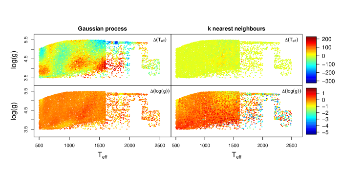
The complete description and analysis of the preliminary set of experiments described in the previous paragraphs is beyond the scope of this article, but the conclusions derived from it can be summarised as follows:

• Residual errors increase near the boundaries of the training sets. The region below 500 K was particularly problematic because prediction errors were unacceptably large and including it in the training sets also degraded the performance for higher temperatures. It was therefore removed from the training sets.

• Denoisification is best achieved by using a moving average filter as measured by the root mean squared reconstruction error (RMSE), and the mean and median reconstruction error.

• The lowest RMSE obtained with wavelet denoising is achieved with the Coiflet mother wavelet of the order of 18; similar RMSE are obtained with the best located wavelet of the order of 14.

• Training the algorithms with a noisy training set adjusted to the signal-to-noise ratios of the test spectrum yields better results than training with noiseless spectra and denoisifying the test spectrum, regardless of the denoisification strategy (moving averages or wavelets).

• Prediction errors obtained with KPLS models are significantly larger (RMSE systematically above 200 K for all G magnitudes and numbers of transits) than those obtained with GP, SVMs, or kNN. models;

• Prediction errors from cross-validation experiments with the various models (except KPLS) and noiseless spectra are all the same within the experimental uncertainty as measured by the standard deviation of the RMSE sample obtained from ten experiments of ten-fold cross validation. The RMSE error for the noiseless training set is 7 K.

• kNN models systematically outperform both SVM and GP models when applied to noisy spectra in the estimation of $T_{\rm eff}$ values. Figure 7 shows a typical case where both the training (nominal) set and the test (random) set were simulated with noise properties for G=20 and 70 transits. The left column shows the distribution of residuals for the GP model ($T_{\rm eff}$ and $\log(g)$ in the upper and lower panel, respectively) and the right column shows the same scatter plots for the kNN model. The RMSE in the $T_{\rm eff}$ predictions is 10 K for the kNN model and 62.3 for the GP model. The RMSE of the kNN model is unrealistically low as shown in the next section, and due in part to the high density of examples in the training set, in this context of cross-validation experiments to derive internal errors. In this setup, where we assumed that the training set of synthetic spectra reproduces the expected observed spectra well , the nearest neighbours are as close as allowed by the density of the grid of training examples (given the relatively high signal-to-noise ratio of the end-of-mission spectra). The performance of the SVM model is overall very similar to that of the GP model.

• Reducing the input space dimensionality with PCA (preserving 95% of the variance) deteriorates the model performances by up to 100% with respect to the complete input spectra. This is so except for the lower signal-to-noise ratios (G=20) and in the combination of PCA and kNN, where the RMSE improves by a 30%. The improvement decreases as the noise diminishes and for G=15, the two models (with and without PCA compression) show the same RMSE. Data compression with the nonlinear technique known as diffusion maps (Coifman & Lafon 2006) results in similar performances as the PCA approach at a much higher computational cost.

In Sect. 4 we concentrate on the external validation of the kNN and GP models only, because the SVM model performances are remarkably similar to the GP models, but do not provide estimates of the prediction uncertainty in a straightforward way. As a result of the previous considerations, we have several regression models based on the $k$-nearest neighbours algorithm and GP. There is a version of each model for the 28 and 70 transits cases, and for the various signal-to-noise ratios that correspond to values of the G magnitude G=15, 18, 19, and 20. For each of these cases we have a model trained in the full input space, or on a PCA compressed version of it. All parameters of each model, such as the number of nearest neighbours or the kernel and noise parameters for the GP models, are determined using ten-fold cross-validation of the models obtained in an exhaustive exploration of the parameter space. The resulting models are used in section 4 to analyse the expected uncertainties when applied to spectra of ultra-cool dwarfs observed from ground and simulated with GOG.

Unfortunately, the internal validation described above for the kNN and GP models overestimates the real accuracy because it does not include several systematic effects. The physical models used in constructing of the training set (AMES-Cond, AMES-Dusty, and BT-Settl) do not exactly reproduce all spectral features and their correlation with the physical parameters encountered in reality. This may be due to several reasons, such as incomplete line lists, inaccurate line/band opacities, or mathematical simplifications introduced for the sake of tractability (e.g. in the dust cloud formation and convection, in the diffusion of chemical species, in the departures from equilibrium between the dust and gas phases, or in the neglect of rotation). To account for these systematic errors, a second battery of experiments is discussed in section 4 where ground-based spectra of well-known ultra-cool stars are degraded to the Gaia resolution and are convolved with its spectral response and error model using GOG. We aim at estimating the error that affects each of the regression models in the various $T_{\rm eff}$ and $\log(g)$ ranges covered by the empirical spectral libraries. The spectra used for the external validation of the regression models are described in detail in the next section.

4 Validation with real spectra

In this section, we use ground-based spectra to estimate the total errors of the regression models. These total errors include the internal validation errors described in the previous section, and errors due to the imperfect representation of real spectra by synthetic models. The ground-based spectra used for validating the regression models are the compilations by A. Reid (Burgasser et al. 2000; Delfosse et al. 1997; Gizis et al. 2000b, a; Kirkpatrick et al. 1999, 2000; Reid et al. 1999, 2000; Strauss et al. 1999; Tsvetanov et al. 2000), S. Leggett (Chiu et al. 2006; Golimowski et al. 2004; Knapp et al. 2004), the NIRSPEC Brown Dwarf Spectroscopic Survey (McLean et al. 2003), and the IRTF spectral library (Cushing et al. 2005; Rayner et al. 2009). None of the observed spectra covers the full Gaia wavelength range,which is especially due to the lack of optical observations at the coolest end. Therefore, it was necessary to complete them with models before simulating the Gaia observations of these stars for ad hoc G magnitudes (and therefore noise levels) and total number of transits. This was accomplished by degrading the resolution of the model spectra to that of the observed spectrum and finding the model that yields the minimum $\chi^{2}$ fit in the wavelength range of overlap restricted to the RP passband (after removing artefacts and wavelength ranges with poor signal-to-noise ratios). This model was then used to complete the observed spectrum. We used all available models from the COND, DUSTY, and BT-Settl libraries to find the best-fitting model to each of the observations, and in all cases the BT-Settl model produced a $\chi^{2}$ statistic superior or comparable to the COND/DUSTY models. Spectra with gaps, small overlap with the RP band, or very low signal-to-noise ratios were removed from this empirical validation set to avoid biases.

The best $\chi^{2}$ fits to the full resolution spectra give us a lower limit to the errors attainable in the Gaia $T_{\rm eff}$ estimates. Figure 8 shows in the $y$-axis the effective temperatures derived from the best $\chi^{2}$ fits described in the previous paragraph as a function of the spectral types assigned in the libraries. We introduced a small jitter (characterised by a standard deviation equal to 30K) in the values of the fitted temperature to enhance the visibility of the stars with the same spectral type. In the same plot we have included the calibration of effective temperatures with spectral types by Stephens et al. (2009) as a continuous line. It corresponds to the calibration derived from optical spectral types of L dwarfs and infrared spectral types of the T dwarfs, valid in the M6 to T8 range (the SLC calibration). The SLC calibration relies on model atmospheres described in Saumon & Marley (2008), and references therein. The dashed lines correspond to the same calibration plus/minus 250 K. The right-hand panel shows the difference between the predicted temperature and the temperature obtained applying the SLC calibration to the spectral types assigned in the compilations, as a function of the latter. The scatter of $T_{\rm eff}$ values in Fig. 8 around the SLC calibration reflects errors of the regression process, but also the uncertainty in the calibration between spectral types and effective temperatures. In this work, we are taking the effective temperature derived through the SLC relation as the ground truth. However, the SLC relation, derived from high-resolution infrared spectra, which are much more appropriate for determining an effective temperature than the Gaia spectrophotometry, has an intrinsic scatter estimated by the authors as $\approx 100K$ (although the article lacks details about how the scatter was estimated, and visual inspection of the plots suggests a much higher scatter at least in the L sequence). Furthermore, Reylé et al. (2011) compared a calibration derived from the BT-Settl model library (the one used in this work) with several other calibrations for the M spectral subsequence in the literature, and found variations of the order of 200-300 K for each spectral subtype. Bayo et al. (2011) showed even higher values of the scatter for the same spectral type range (they derived the $T_{\rm eff}$ values from global fits to the SED). This shows that the calibration of the relationship between effective temperatures and spectral types is a problem that is not yet fully solved, and that the exact $T_{\rm eff}$ values derived for an UCD depend on the calibration used, with typical uncertainties of a few hundred Kelvin. The predictions of the regression modules presented in this section have to be judged in this context. In this respect, our regression models for the Gaia data have the advantage that they will provide UCD temperatures derived consistently from the BT-Settl model family.

Three stars lacked precise spectral subtypes in the spectral compilations, namely 2MASS 1237392+652615, SDSS1346464-003150, and SDSS1624144+002916. We assumed them to be T6.5 (Kirkpatrick et al. 2011), T6.5 (Reylé et al. 2010), and T6 (Kirkpatrick et al. 2011). Figure 8 shows a tendency to assign effective temperatures around 1700 K for sources with spectral type L.

Figure 8: Effective temperatures derived from the best $\chi^{2}$ fits to BT-Settl models as a function of the spectral type assigned in the literature. Black circles correspond to the compilation by Leggett, red circles to the compilation of Keck LRIS spectra by Reid, orange circles to the NIRSPEC compilation, and blue ones to the IRTF compilation. The grey continuous line shows the $T_{\rm eff}$-spectral type calibration by Stephens et al. (2009) from optical and infrared spectra. The dashed lines represent the same calibration $\pm$ 250 K. The right-hand panel shows the residuals ($T_{\rm eff}$_(predicted)-$T_{\rm eff}$_(SLC)) with respect to the calibration.

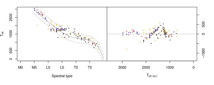
Table 2 lists the mean difference $\mu$ between the $\chi^{2}$ $T_{\rm eff}$ estimates and the effective temperatures derived from the SLC calibration and the spectral types cited in the spectral compilations (hereafter bias); the standard deviation with respect to the bias-corrected mean ($\sigma$) displayed by the four compilations; and the RMSE without correcting for the mean bias. We list these values for the two model families (AMES Cond + Dusty and BT-Settl) used in this work. All RMSE values are given in Kelvin.

Table 2: Average bias ($\mu$) and standard deviation of the $\chi^{2}$ effective temperature (K) fits.

Library	$\mu$ (BT-Settl)	$\sigma$ (BT-Settl)	RMSE (BT-Settl)	$\mu$ (AMES)	$\sigma$ (AMES)	RMSE (AMES)
Leggett	42	196	199	156	197	250
Reid	41	72	143	-84	116	235
NIRSPEC	67	177	256	63	175	251
IRTF	53	63	126	61	70	140

The compilations by Reid and Leggett have a good overall wavelength coverage in the RP range, and spectra with poor coverage were removed from the validation set. Since the expected emission in the wavelength regions of the RP range not covered by the observed spectra (bluewards of 750 nm) is negligible in the $T_{\rm eff}$ and $\log(g)$ parameter ranges under consideration, we expect the completions to have little or no effect on the subsequent parameter estimation with the models described in the previous section. The NIRSPEC library is in the opposite case, with a majority of spectra starting around 1.1 $\mu$m. At this wavelength, the RP transmission is close to zero, and therefore, the input for the GOG simulations of the Gaia RP spectra in the wavelength region where the transmission is high comes only from a synthetic model (the best $\chi^{2}$ match) that was actually used during the training phase of the algorithms. As a consequence, the errors in the parameter estimates for these stars are overly optimistic. The IRTF library is an intermediate case with most spectra covering the wavelength region above 0.8 $\mu$m where most of the source flux is concentrated. Thus, the completion will not have a relevant impact on the resulting simulated RP spectrum.

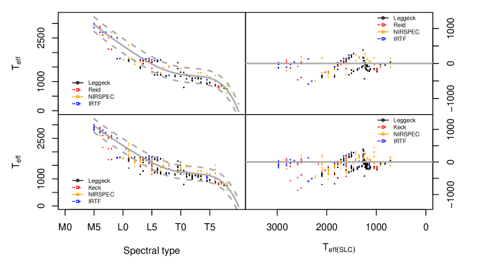
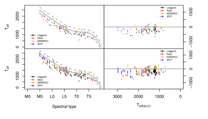
Figures 9 and 10 show the predictions of the kNN and GP models for the empirical libraries described in previous paragraphs. The predicted values of $T_{\rm eff}$ are compared with the effective temperature assigned by the SLC calibration to the spectral type provided by the empirical libraries. The model used in all panels corresponds to the one trained with noisy spectra of G=20 and 70 transits. The upper panels describe the performance of the model when applied to noisy spectra corresponding to G=15 and 70 transits whilst the lower panel shows the results for the same model applied to GOG simulations at G=20 and 70 transits. For each spectrum simulated by GOG, we constructed ten noisy replicates using the Gaia error model currently available, and predict the values of $T_{\rm eff}$ and $\log(g)$ for each one of them. The scatter in the predictions for these noisy replicates is better visible in the lower panels (spectra simulated at G=20).

Figure 9: $T_{\rm eff}$ predictions obtained by the kNN algorithm based on the BT-Settl grid of models for the four libraries of ground-based spectra listed in section 4 for G=15 (top row) and G=20 (bottom row). The colour code is the same as used in Fig. 8. The $x$-axis shows the spectral types gathered from the literature cited in the spectral compilations. The grey line shows the $T_{\rm eff}$-spectral type calibration by Stephens et al. (2009) from optical and infrarred spectra ($\pm 250$K, grey dashed lines). The right-hand panels show the residuals with respect to the calibration as in Fig. 8.

Figure 10: $T_{\rm eff}$ predictions obtained by the GP model based on the BT-Settl grid of models for the four libraries of ground-based spectra listed in section 4 for G=15 (top row) and G=20 (bottom row). The colour code is the same as used in Fig. 8. The $x$-axis shows the spectral types gathered from the literature cited in the spectral compilations. The grey line shows the $T_{\rm eff}$-spectral type calibration by Stephens et al. (2009) from optical and infrared spectra ($\pm 250$K, grey dashed lines). The right-hand panels show the residuals with respect to the calibration as in Fig. 8.

Table 3: Root mean square errors (RMSE) of the GP and kNN models for the prediction of $T_{\rm eff}$, applied to the compilations of empirical spectra.

Number of transits	28			70
G	15	18	20	15	18	20
GP-G20	257 (192)	260 (194)	266 (201)	256 (191)	257 (192)	260 (196)
PCA-GP-G20	266 (199)	270 (203)	281 (216)	264 (197)	266 (200)	272 (207)
kNN-G20	209	210	213	207	209	213
PCA-kNN-G20	211	213	215	209	207	210
Bayes BT-Settl	230.5	235.7	239.0	243.4	241.6	239.7
Bayes COND/DUSTY	252.6	252.3	255.0	257.5	257.6	258.0

Table 3 collects the root mean squared errors (RMSE) of the $T_{\rm eff}$ estimates (expressed in Kelvin) obtained by the GP and kNN models trained with a collection of synthetic spectra of the BT-Settl library simulated for an apparent magnitude G=20. The models are then applied to the four libraries of empirical spectra simulated at 28 and 70 transits, and for apparent magnitudes G=15, 18, and 20. The prefix PCA refers to the models built for the input space of principal componets. The values in parenthesis correspond to the RMSE after correcting for the systematic bias in GP predictions. We also include the RMSE of the Bayesian inference modules built from the BT-Settl and COND/DUSTY model libraries for comparison.

4.1 Bayesian inference

Figure 11: $T_{\rm eff}$ predictions obtained from the ellipsoidal samplings (BT-Settl) for the four empirical libraries of ground-based spectra. The colour code is the same as used in Fig. 8. The $x$-axis shows the spectral types gathered from the literature cited in the spectral compilations. The grey line shows the $T_{\rm eff}$-spectral type calibration by Stephens et al. (2009) from optical and infrared spectra ($\pm 250$K, grey dashed lines). The right-hand panels show the residuals with respect to the calibration as in Fig. 8. The top row corresponds to the spectra simulated at G=15 and the bottom row corresponds to the G=20 replicates.

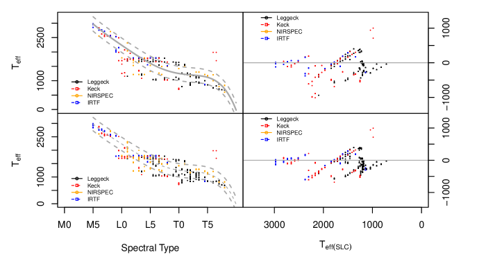
Figure 11 shows the $T_{\rm eff}$ predictions obtained from the ellipsoidal samplings, using the neural network trained with the BT-Settl grid of models and the current error model for the Gaia RP spectra. The predictions are obtained as before, for ten replicates of each GOG simulation of an empirical spectrum. It shows a tendency to predict effective temperatures around 1700 K for stars with spectral type L. Furthermore, there are indications of a second attractor slightly above 1000 K for stars and brown dwarfs with spectral types between L5 and T5. These systematic biases can also be recognised in Figs. 8 (representing the $T_{\rm eff}$ estimates from $\chi^{2}$ fits) and 9 (representing the $T_{\rm eff}$ estimates from $k$-nearest neighbours), but not in Fig. 10 which corresponds to the GP model. The fact that the Bayesian inference shows the same kind of biases as nearest neighbours and the $\chi^{2}$ fits is not surprising because Bayesian inference is equivalent to maximum likelihood estimation under flat priors such as those used in this work. Minimum $\chi^{2}$ fits and nearest neighbours are special cases of maximum likelihood estimation.

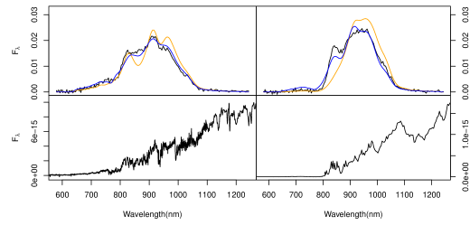
To understand the nature of this trend to concentrate the predictions by the Bayes module around 1700-1800 K, we plot in Fig. 12 the best fits produced by the Bayesian inference module (blue), the model corresponding to the spectral type assigned in the spectral compilations (orange), and finally, one of the ten noisy replicates of the spectrum simulated with GOG for G=20 (black), for two stars with spectral types L1 (left) and T0 (right), both of which are predicted to have temperatures between 1600 and 1700 K. For these two stars we also plot the original spectra for reference (bottom row).

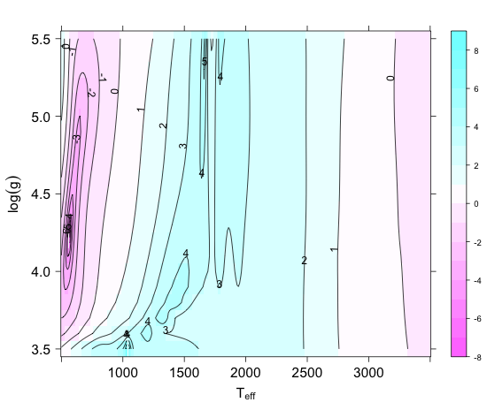
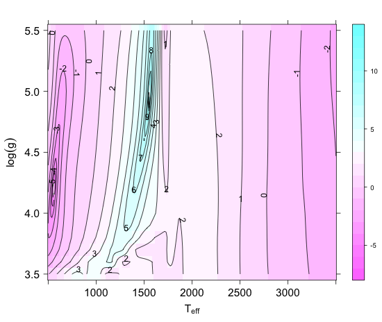
The reason for this systematic effect seems related to the fact that between 1600 and 1800 K, the model spectra undergo, especially at $\log(g)$=5.0, rapid changes with temperature, whilst before and after this range, we find plateaux where the spectra have only a mild dependence with temperature (see Fig. 13). From the sampling perspective, relatively strong changes in the proposed temperatures falling within the plateaux regions result in small changes in the likelihood. Sampling in the 1600-1800 K region on the contrary provides a more varied range of models susceptible to better fit the observed noisy spectrum.

Figure 12: (Top panel, black continuous lines) GOG simulations of spectra contained in the Legget compilation corresponding to 2MASS0345+25 (left) and SDSS1511+06 (right) for G=20 and 70 transits. The blue line represents in both panels the model corresponding to the mode of the posterior probability as derived using ellipsoidal sampling. In orange, the model that corresponds to the effective temperature derived from the spectral type (L1 and T0 respectively) using the SLC calibration. The lower row shows the original spectra completed with the best $\chi^{2}$ model.

Figure 13: BT-Settl model spectra between 1200 and 2000 K (the range of temperatures where the Bayesian module shows a clear tendency to concentrate predictions around 1600-1800 K) and $\log(g)$=5.0. Each panel shows spectra in an interval of temperatures of 200 K. The colour code represents the increment in effective temperature with respect to the lowest temperature covered in the panel. Blue lines correspond to this lowest temperature and red continuous lines correspond to the lowest temperature plus 200 K.

The detailed analysis of the predictions reveals a large variance within some of the blocks of ten noisy replicates of a given spectrum. A good example of this kind of problems is provided by SDSS J010752.33+004156.1, where six estimates cluster around 1036 K whilst the remaining four cluster around 1664 K. As a reference, the spectral type quoted for this object is L5.5 or, equivalently, 1554 K according to the SLC calibration. This apparent inconsistency is due to the multimodal posterior distribution, which is closely related to the likelihood landscape for flat priors and noisy spectra. Figure 14 shows the log-likelihood distribution (derived from one noisy GOG simulation of the spectrum in the Leggett compilation) as a function of the parameters for SDSS J010752.33+004156.1. For comparison, we show the equivalent plot for the model in the BT-Settl grid corresponding to $\bm{\theta}=(1550K,5.0)$ (Fig. 14). Whilst the log-likelihood landscape for the BT-Settl model is unimodal, the log-likelihood landscape for the noisy spectrum of SDSS J010752.33+004156.1 shows maxima of comparable height at 1036 and 1664 K (in addition to other local maxima in the range 1000 K $<$ $T_{\rm eff}$ $<$ 1500 K, 3.5 $<$ $\log(g)$ $<$ 4.0). Depending on the particular realisation of the noise, the ellipsoidal sampling will converge to different maxima. In practice, we find cases of clear bimodality in spectra of stars with spectral types between L1 and T2 ($T_{\rm eff}$ between 1200 and 2000 K).

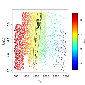
This problem is easily solved by using priors based on the additional information provided by the Gaia astrometric measurements, as suggested in Sect. 3. For this case, Fig. 15 shows a particular choice of the prior that would discard all local maxima that are inconsistent with the Gaia photometry/astrometry, under the assumption of negligible circumstellar and interstellar extinction. In it, we represent the distribution of absolute G magnitudes of the BT-Settl models as a function of the dependent parameters $T_{\rm eff}$ and $\log(g)$. The continuous line shows the 1-$\Sigma$ countour of the two-dimensional Gaussian prior (with $\Sigma$ being the covariance matrix). The prior is fully defined by the mean $\mu_{prior}$ and covariance $\Sigma_{prior}$ of the Gaussian prior distribution. Given a set of astrometric, photometric and spectrophotometric observations such as those simulated for G=20.0 with GOG for SDSS J010752.33+004156.1, and the photometric and astrometric errors shown in Fig. 5, we calculate an absolute G magnitude equal to $19.8492_{-0.0194}^{+0.0191}$, where the uncertainties are derived from the values shown in Fig. 5 multiplied by five. We used five times the nominal uncertainties in the apparent G magnitude and $\pi$ (the parallax) to account for the potential mismatch of the model-predicted magnitudes with respect to the real distribution. We did not take the Lutz-Kelker bias into account in the computation of the uncertainties of the absolute G magnitude. Models within the uncertainties in the absolute G magnitude ($19.8492_{-0.0194}^{+0.0191}$) are shown in Fig. 15 as black circles. We used the $T_{\rm eff}$ and $\log(g)$ parameters of these models to propose the values of $\mu_{prior}$ and $\Sigma_{prior}$ that were used to draw the 1-$\Sigma$ iso-countour in Fig. 15. This prior is eleven orders of magnitude larger at the 1664 K maximum than at the 1036 K one, and thus renders this local maximum insignificant in the posterior probability density distribution. There is a narrow local maximum at $T_{\rm eff}$$\approx$1500 K and $\log(g)$$\approx$4.9 in Fig. 14 where the prior is only one order of magnitude smaller than that corresponding to the 1664 K, but this maximum is never significantly sampled in any of our ten replicates due to its narrowness.

Figure 14: Log-likelihood landscapes for a G=20 noisy replicate of the spectrum of SDSS0107 (left), and the BT-Settl model for 1550 K and $\log(g)$=5.0 (right).

Figure 15: Absolute G magnitudes for the BT-Settl model library as a function of the physical parameters $T_{\rm eff}$ and $\log(g)$ (see colour code at the right-hand side of the scatter plot). Models within $G_{\rm abs}=19.8492_{-0.0194}^{+0.0191}$ (corresponding to SDSS J010752.33+004156.1 simulated at G=20.0) are shown as black circles. The ellipse shows the 1-$\Sigma$ iso-contour of the Gaussian physical prior described in the text.

4.2 Model selection

Ellipsoidal sampling allows estimating the evidence given an observed spectrum and a model choice (COND+DUSTY or BT-Settl), as defined in Eq. 2. Therefore, it is possible to compare these two model families from a Bayesian perspective. $M_{0}$ denotes the BT-Settl model library and $M_{1}$ the COND+DUSTY library. If these were the only two alternatives, then the Bayes factor (BF) in support of the $M_{0}$ model would be defined as the ratio of the respective marginal densities (evidences) of the data for the two models,

$$BF=\frac{m_{0}(\mathbf{s})}{m_{1}(\mathbf{s})}.$$ (6)

If $\pi_{0}$ and $\pi_{1}$ denote the respective prior probabilities (in our case $\pi_{0}=\pi_{1}=1/2$), the posterior probability of $M_{0}$ is given by

$$\Pr(M_{0}|\mathbf{s})=\frac{\pi_{0}BF}{\pi_{0}BF+\pi_{1}}.$$ (7)

We obtain that 73.4 % of the spectra support the BT-Settl model library against 26.6 % supporting the COND-DUSTY combination. For this reason we have exemplified the regression results with figures and discussion related to the models obtained with the BT-Settl library.

4.3 Estimates of the gravity

Figure 16 shows the $T_{\rm eff}$–$\log(g)$ diagrams obtained from the three models discussed in this section. The ellipses represent the covariance estimated from the ten noisy replicates at G=15 of each GOG simulations of the empirical spectra. Since we do not have a compilation of surface gravities available to assess the overall validity of the predictions, we compare the regression values with those obtained from the $\chi^{2}$ fitting to the full resolution spectra. Figure 17 shows this comparison. The $\chi^{2}$ fit values are jittered with a Gaussian distribution of standard deviation equal to 0.2 to enhance the visibility. If the $\chi^{2}$ estimates are taken as targets, only the GP model can be used to obtain very rough estimates of the gravity and to tag low-gravity candidates.

The only star in our samples with an indication of low gravity in the comments section of the Dwarf Archives is the NIRSPEC target star 2MASS J1726000+153819. For this star, both the kNN model and the Bayesian estimate agree to assign a value of $\log(g)$=3.5, while the GP model assigns a higher value $\log(g)$=4.1.

Figure 16: $T_{\rm eff}$–$\log(g)$ predictions for the empirical spectral libraries obtained with the GP model (left), the kNN model (middle), and the Bayesian inference (right). The colour code is the same as in Fig. 8. The ellipses correspond to the covariance estimated from ten noisy replicates of the GOG simulated spectra (G=15).

Figure 17: $\log(g)$ predictions for the empirical spectral libraries obtained with the GP model (left), the kNN model (middle), and the Bayesian inference (right), as a function of the $\log(g)$ value of the minimum $\chi^{2}$ fit (jittered with a Gaussian distribution of $\sigma=0.2$). The colour code is the same as in Fig. 8.

5 Conclusions

We have presented the module that will be in charge of detecting and characterising ultra-cool dwarfs in the Gaia database. The module is subject to change and improvement, but this implementation provides the baseline performance that can be expected from it.

We used the current instrument models and the estimated spatial densities by Caballero et al. (2008) to predict the expected number of ultra-cool dwarfs per spectral type bin. We found that Gaia will be able to detect significant numbers (around or above ten detections) for UCDs of spectral types hotter than L6-7 v. We also used the BT-Settl library of synthetic spectra to define selection criteria for the UCD module such that no UCD is missed due to measurement errors. Given the spatial densities estimated by Caballero et al. (2008), we derived contamination rates from stars hotter than 2500 K in the resulting samples.

We conducted an extensive study to find the best statistical regression model of the relationship between the observed Gaia RP spectrum and the source physical parameters ($T_{\rm eff}$ and $\log(g)$). We evaluated several alternatives in view of their internal and external errors. The internal errors were estimated with cross validation experiments with a dataset interpolated from the nominal grid of models provided by the libraries of synthetic spectra. The external validation was carried out by applying the regression models to an independent set of UCD spectra observed from the ground. All these experiments were carried out on GOG simulations of the full-resolution spectra for a number of apparent G magnitudes and numbers of transits.

As a result, we found that the expected end-of-mission error of the UCD module for the faintest detectable UCDs (G=20) is 210 K for the kNN module and 260 for the GP module (207 K if a bias correction is applied). These performances are approximately constant as a function of G, at least down to G=15 (a typical apparent magnitude for the brightest UCDs in the Gaia catalogue), and are remarkably close to the performance of a simple $\chi^{2}$ fit with the full-resolution spectrum.

The Bayesian inference of the source parameters shows systematic deviations in the distribution of predicted temperatures, which are also apparent (although less conspicuous) in the $\chi^{2}$ fits and kNN predictions. It is also severely affected by the multimodality of the likelihood maps. The application of physical priors and advanced sampling techniques capable of identifying multiple modes in the posterior will be the subject of a forthcoming paper in this series.

The logg predictions are characterised by a typical RMSE of 0.2 dex for the GP module (0.7 dex for the kNN module) as measured by the cross-validation experiments. Unfortunately, these error estimates are overly optimistic because they are derived from testing the regression modules on synthetic spectra and not on observed spectra of real UCDs. The $\log(g)$ estimates for the empirical spectra observed from the ground, although broadly consistent with the expected distribution of values in the samples of empirical spectra, prove that the errors quoted above are indeed extremely optimistic. The GP module will undoubtedly benefit from a more realistic (i.e. wavelength-dependent) treatment of the noise parameter.