Application of Simulated Tempering and Magnetizing to a Two-Dimensional Potts Model

Abstract

We applied the simulated tempering and magnetizing (STM) method to the two-dimensional three-state Potts model in an external magnetic field in order to perform further investigations of the STM’s applicability. The temperature as well as the external field are treated as dynamical variables updated during the STM simulations. After we obtained adequate information for several lattice sizes $L$ (up to $160\times 160$), we also performed a number of conventional canonical simulations of large lattices, especially in order to illustrate the crossover behavior of the Potts model in external field with increasing $L$. The temperature and external field for larger lattice size simulations were chosen by extrapolation of the detail information obtained by STM. We carefully analyzed the crossover scaling at the phase transitions with respect to the lattice size as well as the temperature and external field. The crossover behavior is clearly observed in the simulations in agreement with theoretical predictions.

1 Introduction

Monte Carlo (MC) and molecular dynamics (MD) methods have been demonstrated in many applications to be indispensable tools to study the statistical properties of various systems in equilibrium. The quasi-ergodicity problem, however, where the system gets trapped in states of local energy minima, has often posed great difficulties. In order to overcome this difficulty, generalized-ensemble algorithms have been developed and applied to many problems including spin models and biomolecular systems (for reviews, see, e.g., Refs. [1, 2, 3, 4]).

Well-known examples of generalized-ensemble algorithms are the multicanonical algorithm (MUCA) [5, 6], simulated tempering (ST) [7, 8], and the replica-exchange method (REM) [9, 10] (also referred to as parallel tempering). Closely related to MUCA are the Wang-Landau method [11, 12] and metadynamics [13]. REM is implicitly a special case of the general method described in the earlier work of Ref. [14], as detailed later in Ref. [15].

Based on the recent multi-dimensional generalization of generalized-ensemble algorithms [16, 17, 18], the “Simulated Tempering and Magnetizing” (STM) method has been proposed and developed [19, 20]. In Refs. [19, 20] two of us studied the classical Ising model, introducing the external (magnetic) field as a second dynamical variable besides the temperature and showed improvements over the conventional “one-dimensional” simulated tempering schemes, such as better sampling efficiency and potential applicability to a first-order phase transition, which cannot be dealt with by one-dimensional ST.

In the present work, we further investigate the STM method, applying it to the two-dimensional three-state Potts model in external magnetic field [21, 22]. This model has several interesting applications in condensed matter physics [22] and its three-dimensional counterpart serves as an effective model for quantum chromodynamics [23, 24, 25, 26]. We see the STM scheme working in this more complicated system as well. We also look into crossover behaviors according to lattice size $L$ as well as temperature $T$ and external field $h$. We observe that the STM method lets us investigate a wide area of sampling space.

The rest of this article is organized as follows. In section 2 we review the STM method and give the details of our simulations. In section 3 we present the results. After checking the two-dimensional random walks, we compare ST and STM, and calculate various thermodynamic quantities at many sets of parameter values, in combination with reweighting techniques. We then use this extensive data set to study the crossover scaling behavior at the phase transitions with respect to the lattice size as well as the temperature and external field. In section 4 we conclude this article.

2 Model and Methods

2.1 Model

We study the two-dimensional three-state standard Potts model in external field with energy

$$H =E-hM\,,$$ (1)

$$E =-\sum_{\left<i,j\right>}\delta_{\sigma_{i},\sigma_{j}}\,,$$ (2)

$$M =\sum_{i=1}^{N}\delta_{0,\sigma_{i}}\,,$$ (3)

where $N=L^{2}$ denotes the total number of spins, $\delta$ is the Kronecker delta function, $\sigma_{i}$ a spin at the $i$-th site, and $h$ the external field. The spin $\sigma_{i}$ takes on one of the three values $0$, $1$, or $2$. The sum in (2) goes over all nearest-neighbor pairs, where the spins are arranged on a square $L\times L$ lattice with periodic boundary conditions. Data were obtained in STM for lattice sizes ranging from $2\times 2$ to $160\times 160$ and additionally in conventional canonical simulations on $320\times 320$ and $640\times 640$ lattices.

We recall that the three-state (standard) Potts model is equivalent to the three-state planar Potts or $Z_{3}$ model. We first introduce a spin

$$\vec{s}_{i} =\left(\begin{matrix}\cos\frac{2\pi}{3}\sigma_{i}\\ \sin\frac{2\pi}{3}\sigma_{i}\end{matrix}\right).$$ (4)

The zero-field energy term is then given by

$$E_{\mathrm{planar}}=-\sum_{\left<i,\,j\right>}\vec{s}_{i}\cdot\vec{s}_{j}\,,$$ (5)

and the magnetization reads

$$\vec{M}=\sum_{i=1}^{N}\vec{s}_{i}.$$ (6)

In an external field chosen along the $x$-direction,

$$\vec{h}\equiv h\vec{e}_{x},$$ (7)

the product of external field and magnetization becomes

$$\vec{h}\cdot\vec{M}=hM^{(x)},$$ (8)

where $M^{(x)}$ stands for the $x$-component of $\vec{M}$, which is given by $\sum_{i}\cos\frac{2\pi}{3}\sigma_{i}$. Because the argument of the cosine and sine in (4) can only take the values of $0$, $2\pi/3$, and $4\pi/3$, we have

$$E =\left(E_{\mathrm{planar}}-N\right)\times\frac{2}{3}\,,$$ (9)

$$M =\left(M^{(x)}+\frac{N}{2}\right)\times\frac{2}{3}\,.$$ (10)

Thus, we arrive at

$$E-hM =\frac{2}{3}E_{\mathrm{planar}}-\frac{2}{3}hM^{(x)}-\frac{N}{3}(2-h)\,.$$ (11)

Because the last term is an unimportant constant, the standard Potts model is equivalent to the planar Potts model with a $\frac{2}{3}$-smaller coupling constant and magnetization normalized by $\frac{2}{3}$:

$$H =E-hM\,,$$ (12)

$$E =-\frac{2}{3}\sum_{\left<i,j\right>}\cos\theta_{ij}\,,$$ (13)

$$M =\frac{2}{3}\sum_{i=1}^{N}\cos\theta_{i}\,,$$ (14)

where $\theta_{ij}$ and $\theta_{i}$ are defined by $\theta_{j}-\theta_{i}$ and $\frac{2\pi}{3}\sigma_{i}$, respectively.

Because $M^{(x)}$ is the projection of $\vec{M}$ onto the $x$-axis, $M^{(x)}/N$ equals $1$, $-1/2$, $-1/2$, and $0$ when the system is in the 0-direction ordered, the 1-direction ordered, the 2-direction ordered, and the disordered state, respectively. This corresponds to $M/N=0$ when the system is in 1- or 2-direction ordered states and $M/N=1/3$ in the disordered state.

As one can see from (1) and (3) [or, (12) and (14)], spin direction $0$ is favored by a positive external field ($h>0$). Accordingly, a negative external field ($h<0$) disfavors spin direction $0$. Thus, the system is expected to behave like a two-dimensional Ising model in the presence of a negative external field. In fact, in the limit $h\rightarrow-\infty$, the three-state Potts model is equivalent to the Ising model in zero external field, because the unfavored states disappear in the partition function calculations. Figure 1 illustrates the schematic picture of this relation.

Figure 1: Schematic description of the behavior of spins according to the external field. (a) Spin 0 is favored at $h>0$, i.e., spin 1 and spin 2 are disfavored. (b) All the three states are equivalent at $h=0$. (c) Spin 0 is disfavored at $h<0$.

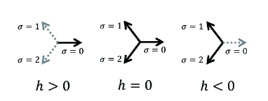
For the easier availability of reference, we summarize the critical exponents for the two-dimensional Ising and three-state Potts model in table 1 [22].

Table 1: Critical exponents for the two-dimensional Ising and three-state Potts models ($y_{t}=1/\nu$, $y_{h}=(\beta+\gamma)/\nu$).

• Model	$y_{t}$	$y_{h}$	$\beta$	$\gamma$	$\delta$	$\nu$
  Ising	1	15/8	1/8	7/4	15	1
  Potts	6/5	28/15	1/9	13/9	14	5/6

2.2 Simulation methods

In this section we briefly review the STM method [19, 20]. While the conventional ST method [7, 8] considers the temperature to be the dynamical variable, the STM method employs the external field as a second dynamical variable besides temperature. This algorithm is based on the multi-dimensional extension of generalized-ensemble algorithms [16, 17, 18]. In other words, we consider

$$\rme^{-(E-hM)/T+a(T,h)}$$ (15)

as a joint probability for $(x,T,h)$ ($\in X\otimes\{T_{1},T_{2},\dots,T_{N_{T}}\}\otimes\{h_{1},h_{2},\dots h_{N_{h}}\}$), where $a(T,h)$, $x$, and $X$ are a parameter, the (microscopic) state, and the sampling space, respectively. Here and hereafter, we set Boltzmann’s constant to unity. Note that the temperature and external field are discretized into $N_{T}$ and $N_{h}$ values, respectively.

We will find the candidate for $a(T_{i},h_{j})$ by looking into the probability of occupying each set of parameter values. It is given by

$$P(T_{i},h_{j}) =\frac{\displaystyle\sum_{k=1}^{N_{T}}\displaystyle\sum_{l=1}^{N_{h}}\int\rmd x\,\delta_{ik}\,\delta_{jl}\,\rme^{-\frac{E(x)-h_{l}M(x)}{T_{k}}+a(T_{k},h_{l})}}{\displaystyle\sum_{k=1}^{N_{T}}\displaystyle\sum_{l=1}^{N_{h}}\int\rmd x\,\rme^{-\frac{E(x)-h_{l}M(x)}{T_{k}}+a(T_{k},h_{l})}}$$ (16)

$$=\frac{\rme^{-f(T_{i},h_{j})+a(T_{i},h_{j})}}{\displaystyle\sum_{k=1}^{N_{T}}\displaystyle\sum_{l=1}^{N_{h}}\rme^{-f(T_{k},h_{l})+a(T_{k},h_{l})}}$$ (17)

$$\propto\rme^{-f(T_{i},h_{j})+a(T_{i},h_{j})}\,,$$ (18)

where

$$\rme^{-f(T_{i},h_{j})}=\int\rmd x\rme^{-(E-h_{j}M)/T_{i}}.$$ (19)

Thus, the dimensionless free energy $f(T_{i},h_{j})$ is a proper choice for $a(T_{i},h_{j})$ in order to acquire a uniform distribution of the number of samples according to $T$ and $h$. These values can be estimated by a number of methods. For example, one can obtain such values from preliminary simulations and reweighting techniques.

Any thermal average $\left<A\right>_{T_{i},h_{j}}$ at given $T_{i}$ ($\in\{T_{1},T_{2},\dots,T_{N_{T}}\}$) and $h_{j}$ ($\in\{h_{1},h_{2},\dots,h_{N_{h}}\}$) can be obtained by the conditional expectation: $\left<A\right>_{T_{i},h_{j}}=\left<A|T_{i},h_{j}\right>_{\mathrm{STM}}$. Namely, we have

$$\left<A\right>_{T_{i},h_{j}}=\frac{1}{N_{T_{i},h_{j}}}\sum_{k=1}^{N_{T_{i},h_{j}}}A^{k}_{T_{i},h_{j}}\,,$$ (20)

where $N_{T_{i},h_{j}}$ is the total number of samples obtained at $T_{i}$ and $h_{j}$, and $A^{k}_{T_{i},h_{j}}$ represents the $k$-th sample at $T_{i}$ and $h_{j}$.

The temperature $T$ or external field $h$ can be updated similarly to the spin $\sigma_{i}$, because they are considered as dynamical variables. The Metropolis criterion for updating $T$ and $h$ is given by

$$w(T_{i},h_{j} \rightarrow T_{i^{\prime}},h_{j^{\prime}})=\min\left(1,\frac{P(T_{i^{\prime}},h_{j^{\prime}})}{P(T_{i},h_{j})}\right)$$ (21)

$$=\min\left(1,\exp\left(-\left(\frac{1}{T_{i^{\prime}}}-\frac{1}{T_{i}}\right)E+\left(\frac{h_{j^{\prime}}}{T_{i^{\prime}}}-\frac{h_{j}}{T_{i}}\right)M+a(T_{i^{\prime}},h_{j^{\prime}})-a(T_{i},h_{j})\right)\right)\,.$$ (22)

Once an initial state is prepared, the STM simulations can be performed by repeating the following two steps: 1. We perform a conventional canonical simulation at fixed $T_{i}$ and $h_{j}$ for a certain number of MC sweeps. 2. We update the temperature and/or external field by (22) with $a(T,h)=f(T,h)$.

In our implementation, every fixed number of MC sweeps, either $T$ or $h$ was updated (the choice between $T$ and $h$ was made at random) by (22) to a neighboring value (the choice between two possible neighbors was also made at random). Here, one MC sweep consists of $L\times L$ single spin updates. The number of MC sweeps performed between parameter updates is here referred to as the parameter-updating period.

We remark that, as spins can be updated by a number of algorithms, other schemes of updating the parameters can be employed [27]. There also exists a temperature updating scheme for ST by the Langevin algorithm [28].

Table 2 summarizes the conditions of the present STM simulations. According to the previous studies [20, 29, 30], we updated the parameters frequently. That is, we employed very small parameter-updating periods.

Table 2: Parameter values for the STM simulations.

Lattice size $L$	5	10	20	40	80	160
Total MC sweeps	220915510	216277330	164000000	164000000	43605000	525000000
Parameter-updating period	1	1	1	1	1	1
$T_{1},\dots,T_{N_{T}}$	$0.1,\dots,3.5$	$0.1,\dots,3.5$	$0.3,\dots,3.2$	$0.3,\dots,3.2$	$0.5,\dots,2.0$	$0.5,\dots,2.0$
$h_{1},\dots,h_{N_{h}}$	$-1.5,\dots,1.5$	$-1.5,\dots,1.5$	$-1.5,\dots,1.5$	$-1.5,\dots,1.5$	$-1.5,\dots,1.5$	$-1.0,\dots,0.025$
$N_{T}$	20	20	40	40	76	95
$N_{h}$	21	21	41	41	5 1	30
$N_{{\rm data}}$ a	10	10	10	10	10	10

^a The data were stored every $N_{{\rm data}}$ MC sweeps.

In addition, we also performed conventional canonical simulations. Table 3 lists their details. The temperature was chosen by extrapolations of the STM results. We estimated the proper temperature by fitting the STM results to $T_{\mathrm{max}}-T_{\mathrm{c}}\propto L^{-1/\nu}$, where $T_{\mathrm{max}}$ is the temperature at which the observables take their maxima. The Greek letter $\nu$ denotes the critical exponent of the correlation length. For vanishing external field we fitted the data to the Potts case ($\nu=5/6$) and in (negative) external field to the Ising case ($\nu=1$), respectively.

Table 3: Parameter values for the regular canonical simulations.

Lattice size $L$	320	640
Total MC sweeps a	4000000	4000000
$(T,\,h)$ b	(0.995518, 0), (0.995995, 0), (0.996490, 0)	(0.994985, 0), (0.995209, 0), (0.995512, 0)
	(1.0752077, $-0.5$), (1.077044, $-0.5$), (1.078302, $-0.5$)	(1.075672, $-0.5$), (1.076181, $-0.5$), (1.076936, $-0.5$)
	(1.101447, $-1.0$), (1.102321, $-1.0$), (1.103380, $-1.0$)	(1.100386, $-1.0$), (1.101043, $-1.0$), (1.101811, $-1.0$)
$N_{{\rm data}}$ c	10	20

^a The number performed for each set of temperature and external field.
^b Three temperature values for each external field.
^c The data were stored every $N_{{\rm data}}$ MC sweeps.

As for spin updates, we employed the single-spin update algorithm; we updated spins one by one with the heatbath algorithm. As for quasi-random-number generator, we used the Mersenne Twister [31].

2.3 Free energy calculations

The simulated tempering parameters, or free energy, in (15) and (19) can be simply obtained by reweighting techniques applied to the results of preliminary simulation runs [16, 17, 18, 32]. We used two reweighting methods for the free energy calculations. One method is the multiple-histogram reweighting method, or Weighted Histogram Analysis Method (WHAM) [33, 34, 35] and the other is the Multistate Bennett Acceptance Ratio estimator (MBAR) [36], which is based on WHAM.

The equations of the WHAM algorithm applied to the system are as follows. For details, the reader is referred to Refs. [17, 34, 35]. The density of states (DOS) $n(E,M)$ and free energy values $f(T_{i},h_{j})$ can be obtained from

$$n(E,M) =\frac{\displaystyle\sum_{i=1}^{N_{T}}\displaystyle\sum_{j=1}^{N_{h}}n_{T_{i},h_{j}}(E,M)}{\displaystyle\sum_{i=1}^{N_{T}}\displaystyle\sum_{j=1}^{N_{h}}N_{T_{i},h_{j}}\exp(f(T_{i},h_{j})-(E-h_{j}M)/T_{i})}\,,$$ (23)

$$f(T_{i},h_{j}) =-\ln\sum_{E,M}n(E,M)\exp(-(E-h_{j}M)/T_{i})\,,$$ (24)

where $n_{T_{i},h_{j}}(E,M)$ is the histogram of $E$ and $M$ at $T_{i}$ and $h_{j}$, and $N_{T_{i},h_{j}}$ is the total number of samples obtained at $T_{i}$ and $h_{j}$. By solving these two equations self-consistently by iteration, we can obtain $n(E,M)$ and $f(T_{i},h_{j})$. The obtained $n(E,M)$ allows one to calculate any thermal average at arbitrary temperature and external field values. Note that $f(T_{i},h_{j})$ is determined up to a constant, which sets the zero point of free energy. Accordingly, $n(E,M)$ is determined up to a normalization constant.

The MBAR is based on the following equations. Namely, by combing (23) and (24), the free energy can be written as

$$f(T_{i},h_{j})=-\ln\sum_{n=1}^{N}\frac{\exp(-(E_{n}-h_{j}M_{n})/T_{i})}{\displaystyle\sum_{k=1}^{N_{T}}\displaystyle\sum_{l=1}^{N_{h}}N_{T_{k},h_{l}}\exp(f(T_{k},h_{l})-(E_{n}-h_{l}M_{n})/T_{k})}\,,$$ (25)

where $N$, $N_{T_{k},h_{l}}$, $E_{n}$, and $M_{n}$ is the total number of data, the number of samples associated with $T_{k}$ and $h_{l}$, energy of the $n$-th data, and magnetization of the $n$-th data, respectively. This equation should be solved self-consistently for $f(T_{i},h_{j})$. Note that, as in WHAM, $f(T_{i},h_{j})$ is determined up to a constant.

We repeat the preliminary STM simulations and free energy calculations until we finally obtain sufficiently accurate free energy values which let the system perform a random walk in the temperature and external field space during the STM simulation. We then perform a final production run.

Note that these two reweighting methods enable us to obtain not only dimensionless free energy values but also physical values at any temperature and at any external field. Such averages are given by

$$\left<A\right>_{T,h} =\sum_{n=1}^{N}W_{na}A(x_{n})\,,$$ (26)

$$W_{na} =\frac{1}{\left<c_{a}\right>}\frac{\exp(-(E_{n}-hM_{n})/T)}{\displaystyle\sum_{k=1}^{N_{T}}\displaystyle\sum_{l=1}^{N_{h}}N_{T_{k},h_{l}}\exp(f(T_{k},h_{l})-(E_{n}-h_{l}M_{n})/T_{k})}\,,$$ (27)

$$\left<c_{a}\right> =\displaystyle\sum_{n=1}^{N}\frac{\exp(-(E_{n}-hM_{n})/T)}{\displaystyle\sum_{k=1}^{N_{T}}\displaystyle\sum_{l=1}^{N_{h}}N_{T_{k},h_{l}}\exp(f(T_{k},h_{l})-(E_{n}-h_{l}M_{n})/T_{k})}\,.$$ (28)

For details, the reader is referred to Refs. [36, 37].

We also used two other methods of free energy calculations. One is given as follows. By substituting $a(T,h)$ in (18) by the estimates for free energy $\tilde{f}(T,h)$, we obtain

$$P(T,h) \propto e^{-f(T,h)+\tilde{f}(T,h)}.$$ (29)

We can write

$$f(T,h)=\tilde{f}(T,h)-\ln P(T,h)+\rm{const}.$$ (30)

Here, $P(T,h)$ can be obtained as a histogram at each set of parameter values in a preliminary STM simulation. Thus, this equation enables one to refine the free energy much more easily than the reweighting methods, because the method does not require any iterations. This method does not work well, however, when $P(T_{i},h_{j})$ is too small (or $\tilde{f}(T_{i},h_{j})$ is too far away from the true values) to obtain samples at $(T_{i},h_{j})$, while the reweighting techniques still work.

The other method for the free energy calculations is a Wang-Landau-like scheme, where we subtract the free energy value being sampled by a fixed constant during preliminary simulations. To stand on the safe side, we did not use such data for reweighting techniques which, strictly speaking, requires equilibrium data as inputs. Note that this method also works with inaccurate free energy values. Thus, this method works even when the free energy estimates are far away from sufficiently accurate values.

In the present work, we first used the reweighting methods and Wang-Landau-like scheme to obtain rough estimates of the free energy for the entire parameter space. We then used the combination of the reweighting methods and (30) for further refinements of the free energy.

3 Results and Discussion

We first examine whether the STM simulations were carried out properly or not. Figure 3 and figure 3 show the time series of temperature and external field, respectively, for $L=80$. In both plots we see block structures reflecting the first-order phase transition line at $h=0$ in the Potts model (see figure 3) and the second-order phase transition at the effective Ising transition temperature $T_{\mathrm{c}}(h)\approx 1.1346$ for negative external field (see figure 3). Within these blocks, the temperature and external field indeed realized random walks.

Figure 2: History of temperature $T$ for the linear lattice size $L=80$.

Figure 3: History of external field $h$ for the linear lattice size $L=80$.

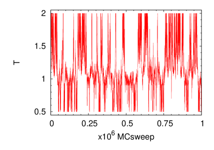
Figure 5 and figure 5 show the energy per spin and the magnetization per spin, respectively, as functions of MC sweeps. They also performed random walks. Note that there exist expected correlations between the temperature and energy (see figures 3 and 5) and between the external field and magnetization (see figures 3 and 5). The same behavior was observed in simulations with other lattice sizes (data not shown).

Figure 4: History of energy per spin, $E/L^{2}$, for the linear lattice size $L=80$.

Figure 5: History of the magnetization per spin, $M/L^{2}$, for the linear lattice size $L=80$. Recall that $M/L^{2}=1$ corresponds to the ordered state in 0-direction, $M/L^{2}=0$ to the ordered states in 1- or 2-direction, and $M/L^{2}=1/3$ to the disordered state.

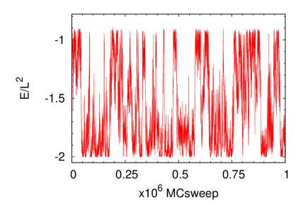
Figure 6 shows the history of a differently defined magnetization given by

$$M_{\mathrm{max}}\equiv\left\{\max_{j=0,1,2}\left[\sum_{i}^{L^{2}}\delta_{j,\sigma_{i}}\right]-\frac{L^{2}}{3}\right\}\times\frac{3}{2}.$$ (31)

Hereafter, we also use the following definition:

$$m_{\mathrm{max}}\equiv\frac{M_{\mathrm{max}}}{L^{2}}.$$ (32)

This quantity takes physically more intuitive values of 1 and 0 when the system is in one of the three ordered phases and in the disordered phase, respectively. Here, we see a clear negative correlation between $E/L^{2}$ and $M_{\mathrm{max}}/L^{2}$ (see figures 5 and 6).

Figure 6: History of $M_{\mathrm{max}}/L^{2}$ ($\equiv m_{\mathrm{max}}$), for the linear lattice size $L=80$.

To compare the results with ordinary ST simulations, we also performed a ST simulation with $L=40$. The ST simulation was performed at the conditions similar to those of STM; namely, the same total number of MC sweeps, same temperature distribution, and so on, except that here we set $h=0$.

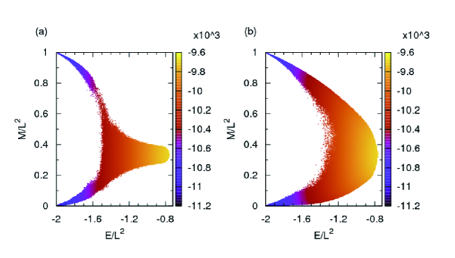
With the data obtained, we performed the WHAM calculations to obtain the DOS. As shown in figure 7, the area sampled by STM is larger than that by ST. Thus, the STM method enables us to perform reweighting techniques in a wider range. We recall that $M$ is zero in the 1- or 2-direction ordered phases. The disordered phase corresponds to $M/L^{2}=\frac{1}{3}$.

Figure 7: Calculated DOS obtained by WHAM with (a) ST and (b) STM data. The linear lattice size $L$ was 80.

We further closely look into the difference in the sampled areas between the two methods. Figure 8 illustrates how the sampled areas differ. The red, green, blue, and white regions correspond to the region that was sampled by the STM method exclusively, by both methods, by the ST method only, and by neither of them, respectively. Thus, at first sight, it seems that there are some areas in which STM is not good and that ST is somehow more powerful than STM.

Figure 8: Difference in sampled points between ST and STM. The red, green, blue, and white regions correspond to the area sampled by only STM, by both of them, only by ST, and by neither of them, respectively ($L=40$).

Figure 9: Difference in sampled points between ST and STM. The red, green, blue, and white regions correspond to the area sampled by only STM, by both of them, only by ST, and by neither of them, respectively. Plots (a) and (b) are with different focus.

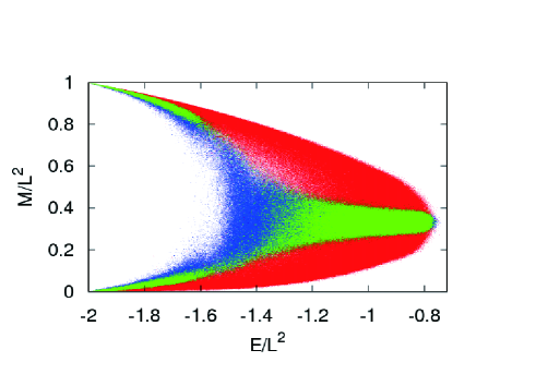
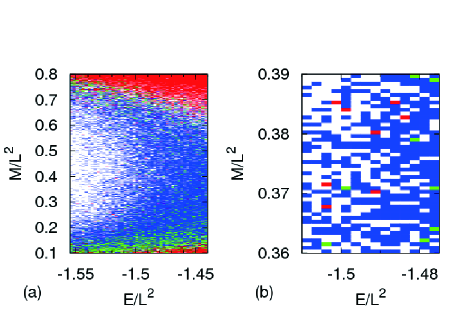
Figure 9 zooms in on a region where blue is dominant (mainly sampled by ST). There are many pigments (in red and green) which both methods sampled and which even only STM sampled. This shows that because the ST method has more samples at a smaller number of parameter values, the part sampled is narrower but denser. However, the representative parts should be sampled properly by STM as well, although the sample density decreases.

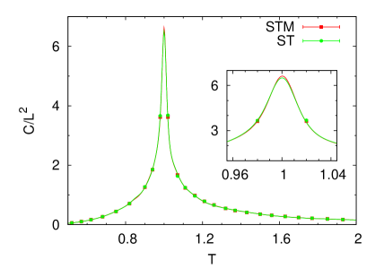
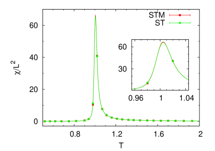
To make it sure that the STM method also samples the relevant area sufficiently, we then performed reweighting analyses along $h=0$ with data obtained by ST and STM. Figure 10 and figure 11 show specific heat $C/L^{2}$ and susceptibility $\chi/L^{2}$, respectively, as functions of $T$ along the line $h=0$. They are defined by

$$C \equiv\frac{\left<E^{2}\right>-\left<E\right>^{2}}{T^{2}}\,,$$ (33)

$$\chi \equiv\frac{\left<M_{\mathrm{max}}^{2}\right>-\left<M_{\mathrm{max}}\right>^{2}}{T}.$$ (34)

The red and green curves correspond to the data obtained by STM and by ST, respectively. The error bars were obtained by the jackknife method [38, 39, 40, 41]. We see no outstanding differences between the two methods. Thus, we confirm that both methods let one sample the representative parts along $h=0$ and that the STM method enables one to obtain the DOS in wider areas.

Figure 10: Specific heat $C/L^{2}$ as a function of $T$ for $L=40$. The inset has different abscissa and ordinate.

Figure 11: Susceptibility $\chi/L^{2}$ as a function of $T$ for $L=40$. The inset has different abscissa and ordinate.

Because the STM method enables us to obtain the DOS in a wide range of sampling space, we can calculate the two-dimensional map of any thermodynamic quantity. Figure 12 shows the specific heat and susceptibility per spin as functions of $T$ and $h$ when $L=80$. This implies that the phase transition temperature converges into the Ising case value of $1.1346$, as the external field decreases. Related theoretical work is found in, e.g., Ref. [42].

Figure 12: (a) $C/L^{2}$ and (b) $\chi/L^{2}$ as functions of $T$ and $h$ for $L=80$. The solid vertical line corresponds to $T=1.1346$, which is the critical temperature of the Ising model (in Potts model normalization).

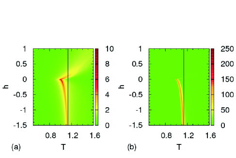
Figure 13 shows the specific heat as a function of temperature for some values of $h$ and $L$. With positive external field, the phase transition disappears. However, because of finite effects, the abnormality, as measured by the diverging behavior, persists to some extent. With smaller external field, the divergence behavior remains for larger $L$. Vice versa, with larger $L$, the more easily it can be shown that the diverging behavior disappears. This can be seen as a crossover between $L$ and $h$.

Figure 13: Specific heat $C/L^{2}$ as a function of $T$ for $L=5$ (red), $10$ (green), $20$ (blue), $40$ (magenta), and $80$ (cyan). (a) $h=0.0$, (b) $h=0.005$, (c) h=$0.01$ (d) $h=0.02$.

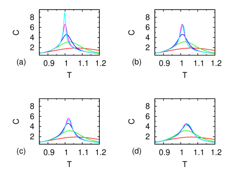
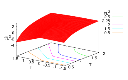
Figure 14 shows the dimensionless free energy per spin as a function of temperature and external field, which was obtained by applying MBAR to the results of the production runs. Note that the partial derivative of this free energy with respect to $h$ gives $\frac{\left<M\right>}{TL^{2}}$, where $\left<M\right>$ is defined in (3). The shape at $h=0$ suggests a jump of $m$ below $T_{\mathrm{c}}$, indicating the existence of first-order phase transitions.

Figure 14: Free energy per spin $f/L^{2}$ and its contour curves as a function of $T$ and $h$. The linear lattice size $L$ was 80.

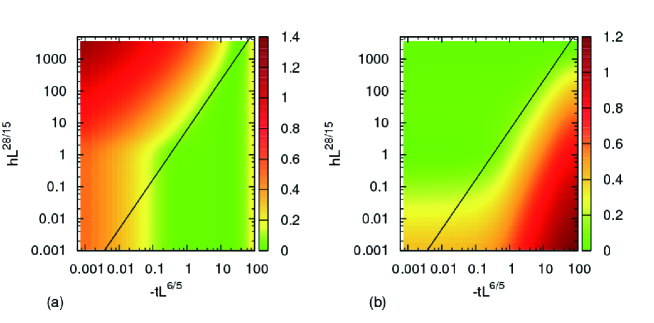
Finally to study the crossover behavior of the phase transitions, we calculated the magnetization by MBAR around the critical point. The scaling form of $m$ is given by [43]

$$mL^{\beta/\nu}=\Psi(tL^{y_{t}},hL^{y_{h}}),$$ (35)

where $y_{t}=1/\nu$ and $y_{h}=(\beta+\gamma)/\nu$. According to the crossover scaling formalism [43], if $t^{-\frac{y_{h}}{y_{t}}}h$ (in Potts model $t^{-14/9}h$) is small enough, then the magnetization obeys $m\sim t^{1/9}$($=t^{\beta}$), and if $h^{-\frac{y_{t}}{y_{h}}}t$ (in Potts model $h^{-9/14}t$) is small enough (i.e., $t^{-14/9}h$ is large enough), then it obeys $m\sim h^{1/14}$ ($=h^{1/\delta}$), where $t=\frac{T-T_{\mathrm{c}}}{T_{\mathrm{c}}}$. Figure 15(a) shows that if the finite-size effects are negligible ($L^{6/5}t\gg 0.1$) and $t\gg(1/6)h^{9/14}$ (i.e., $t^{-14/9}h$ is small), then the critical behavior is $m\sim t^{1/9}$. Figure 15(b) shows that if finite-size effects are negligible ($L^{28/15}h\gg 0.1$) and $t\ll(1/6)h^{9/14}$ (i.e., $t^{-14/9}h$ is large), then the critical behavior is $m\sim h^{1/14}$. Thus, figure 15 clearly shows that the line ($t=(1/6)h^{9/14}$) gives the boundary of the two scaling regimes.

Figure 15: Difference between magnetization and its expected scaling behaviors around the critical point. The linear lattice size $L$ was 80. (a) $|mL^{2/15}-1.2(L^{6/5}t)^{1/9}|$ is illustrated. The solid line corresponds to $h=6t^{14/9}$. (b) $|mL^{2/15}-(L^{28/15}h)^{1/14}|$ is illustrated. The solid line corresponds to $h=6t^{14/9}$.

Because the three-state Potts model in a negative external field is expected to behave like the Ising model, we also investigated the crossover behavior between the two models. The scaling exponents of $\chi_{\mathrm{max}}$ for increasing $L$ of the Potts model and the Ising model are given by $\gamma/\nu={26/15}$ and $7/4$, respectively. Figure 16 shows that the exponents are so similar that we cannot distinguish the difference, despite the accuracy of the measurements.

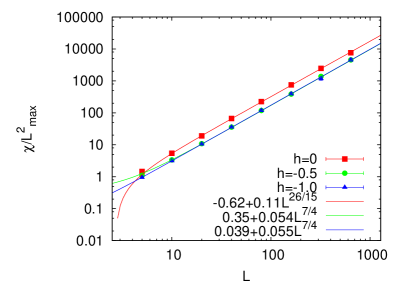
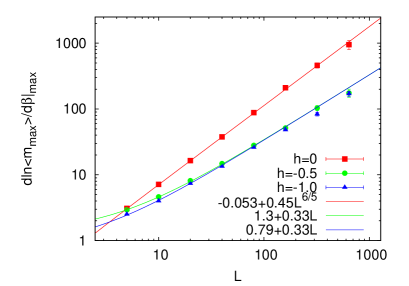
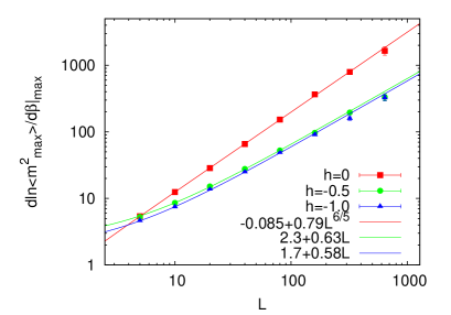
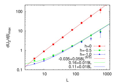
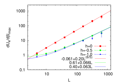
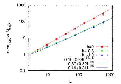
Thus, we measured different quantities, which are the maximum values of $\frac{\rmd\ln\left<m_{\mathrm{max}}\right>}{\rmd\beta}$, $\frac{\rmd\ln\left<m_{\mathrm{max}}^{2}\right>}{\rmd\beta}$, $\frac{\rmd\ln\left<U_{2}\right>}{\rmd\beta}$, $\frac{\rmd\ln\left<U_{4}\right>}{\rmd\beta}$, and $\frac{\rmd\left<m_{\mathrm{max}}\right>}{\rmd\beta}$. Here, $U_{2}=1-\frac{\left<m^{2}_{\mathrm{max}}\right>}{3\left<m_{\mathrm{max}}\right>^{2}}$ and $U_{4}=1-\frac{\left<m^{4}_{\mathrm{max}}\right>}{3\left<m^{2}_{\mathrm{max}}\right>^{2}}$ are the Binder cumulants [44]. These quantities were measured by [45]

$$\noindent\frac{\rmd\ln\left<m_{\mathrm{max}}\right>}{\rmd\beta} =\left<E\right>-\frac{\left<m_{\mathrm{max}}E\right>}{\left<m_{\mathrm{max}}\right>},$$ (36)

$$\frac{\rmd\ln\left<m_{\mathrm{max}}^{2}\right>}{\rmd\beta} =\left<E\right>-\frac{\left<m^{2}_{\mathrm{max}}E\right>}{\left<m^{2}_{\mathrm{max}}\right>},$$ (37)

$$\frac{\rmd\ln\left<U_{2}\right>}{\rmd\beta} =\frac{\left<m_{\mathrm{max}}^{2}\right>}{3\left<m_{\mathrm{max}}\right>^{2}}\left\{\left<E\right>-2\frac{\left<m_{\mathrm{max}}E\right>}{\left<m_{\mathrm{max}}\right>}+\frac{\left<m^{2}_{\mathrm{max}}E\right>}{\left<m^{2}_{\mathrm{max}}\right>}\right\},$$ (38)

$$\frac{\rmd\ln\left<U_{4}\right>}{\rmd\beta} =\frac{\left<m_{\mathrm{max}}^{4}\right>}{3\left<m_{\mathrm{max}}^{2}\right>^{2}}\left\{\left<E\right>-2\frac{\left<m^{2}_{\mathrm{max}}E\right>}{\left<m^{2}_{\mathrm{max}}\right>}+\frac{\left<m^{4}_{\mathrm{max}}E\right>}{\left<m^{4}_{\mathrm{max}}\right>}\right\},$$ (39)

$$\frac{\rmd\left<m_{\mathrm{max}}\right>}{\rmd\beta} =\left<m_{\mathrm{max}}\right>\left<E\right>-\left<m_{\mathrm{max}}E\right>.$$ (40)

Figures 17–21 show the results. Note that $\frac{\rmd\ln\left<m_{\mathrm{max}}\right>}{\rmd\beta}|_{\mathrm{max}}$, $\frac{\rmd\ln\left<m_{\mathrm{max}}^{2}\right>}{\rmd\beta}|_{\mathrm{max}}$, $\frac{\rmd\ln\left<U_{2}\right>}{\rmd\beta}|_{\mathrm{max}}$, $\frac{\rmd\ln\left<U_{4}\right>}{\rmd\beta}|_{\mathrm{max}}$, and $\frac{\rmd\left<m_{\mathrm{max}}\right>}{\rmd\beta}|_{\mathrm{max}}$ are expected to behave asymptotically as $L^{1/\nu}$, $L^{1/\nu}$, $L^{1/\nu}$, $L^{1/\nu}$, and $L^{(1-\beta)/\nu}$, respectively, as the lattice size $L$ increases [41]. These critical exponents for the Potts model and the two-dimensional Ising model are given by $\nu=\frac{5}{6}$ and $\beta=\frac{1}{9}$ so that $(1-\beta)/\nu=16/15$ and $\nu=1$ and $\beta=\frac{1}{8}$ so that $(1-\beta)/\nu=7/8$ , respectively. We observe that all quantities along $h=0$ (red curve with filled squares) follow the Potts case, and those with the external field at large $L$ (green curve with filled circles and blue curve with filled triangles) follow the Ising case. Note that the two curves at $h=-0.5$ and $h=-1.0$ converge into almost the same line as $L$ increases. On the other hand, the curve at $h=-0.5$ (green curve) is more deviating from the scaling behavior. This can also be understood as the crossover between $L$ and $h$.

Figure 16: $\chi_{\mathrm{max}}/L^{2}$ as functions of $L$.

Figure 17: $\frac{\rmd\ln\left<m_{\mathrm{max}}\right>}{\rmd\beta}|_{\mathrm{max}}$ as functions of $L$.

Figure 18: $\frac{\rmd\ln\left<m_{\mathrm{max}}^{2}\right>}{\rmd\beta}|_{\mathrm{max}}$ as functions of $L$.

Figure 19: $\frac{\rmd\ln\left<U_{2}\right>}{\rmd\beta}|_{\mathrm{max}}$ as functions of $L$.

Figure 20: $\frac{\rmd\ln\left<U_{4}\right>}{\rmd\beta}|_{\mathrm{max}}$ as functions of $L$.

Figure 21: $\frac{\rmd\left<m_{\mathrm{max}}\right>}{\rmd\beta}|_{\mathrm{max}}$ as functions of $L$.

4 Conclusions

In this work, we applied Simulated Tempering and Magnetizing (STM) [19, 20] to the two-dimensional three-state Potts model. During the simulations, two-dimensional random walks in temperature and external field were realized. The random walk covered a wide area of temperature and external field so that the STM simulations enabled us to study a wide area of the phase diagram from a single simulation run.

Because of the method’s capability of dealing with a wider area of the sampling space (as is seen in DOS), we can calculate thermodynamic quantities at an enlarged range of the parameter space. We succeeded in reproducing many typical features of the system in the presence of an external field.

We investigated the crossover behavior of the phase transitions by calculating the magnetization per spin $m$ around the critical point by reweighting techniques. The results showed agreement with previous theoretical studies. Thus, this supports the validity of the two-dimensional ST method, or STM.

With the data of the present work, we can calculate the two-dimensional density of states $n(E,M)$ so that we can determine the weight factor for two-dimensional multicanonical simulations. Therefore, we can also perform two-dimensional multicanonical simulations which would be an interesting future task.

We also remark that the present methods are useful not only for spin systems but also for other complex systems with many degrees of freedom. Note that because this method does not require one to change the energy calculations, the method should be highly compatible with existing program packages.

References

- [1] W. Janke. Multicanonical Monte Carlo simulations. Physica A: Statistical Mechanics and its Applications, 254:164–178, 1998.
- [2] U. H. E. Hansmann and Y. Okamoto. The generalized-ensemble approach for protein folding simulations. In Dietrich Stauffer, editor, Annual Reviews of Computational Physics VI, pages 129–157. World Scientific, Singapore, 1999.
- [3] A. Mitsutake, Y. Sugita, and Y. Okamoto. Generalized-ensemble algorithms for molecular simulations of biopolymers. Biopolymers, 60(2):96–123, 2001.
- [4] W. Janke, editor. Rugged Free Energy Landscapes: Common Computational Approaches to Spin Glasses, Structural Glasses and Biological Macromolecules, volume 736. Springer, Berlin, 2008. Lecture Notes in Physics.
- [5] B. A. Berg and T. Neuhaus. Multicanonical algorithms for first order phase transitions. Physics Letters B, 267(2):249–253, 1991.
- [6] B. A. Berg and T. Neuhaus. Multicanonical ensemble: A new approach to simulate first-order phase transitions. Physical Review Letters, 68(1):9–12, 1992.
- [7] A. P. Lyubartsev, A. A. Martsinovski, S. V. Shevkunov, and P. N. Vorontsov-Velyaminov. New approach to Monte Carlo calculation of the free energy: Method of expanded ensembles. The Journal of Chemical Physics, 96(3):1776, 1992.
- [8] E. Marinari and G. Parisi. Simulated tempering: A new Monte Carlo scheme. Europhysics Letters, 19(6):451–458, 1992.
- [9] K. Hukushima and K. Nemoto. Exchange Monte Carlo method and application to spin glass simulations. Journal of the Physics Society Japan, 65(6):1604–1608, 1996.
- [10] C. J. Geyer. In E. M. Keramidas, editor, Computing Science and Statistics, Proceedings of the 23rd Symposium on the Interface, pages 156–163. Interface Foundation of North America, 1991.
- [11] F. Wang and D. P. Landau. Efficient, multiple-range random walk algorithm to calculate the density of states. Physical Review Letters, 86:2050–2053, 2001.
- [12] F. Wang and D. P. Landau. Determining the density of states for classical statistical models: A random walk algorithm to produce a flat histogram. Physical Review E, 64:056101, 2001.
- [13] A. Laio and M. Parrinello. Escaping free-energy minima. Proc. Natl. Acad. Sci. USA, 99:12562–12566, 2002.
- [14] R. H. Swendsen and J.-S. Wang. Replica Monte Carlo simulation of spin-glasses. Physical Review Letters, 57:2607–2609, 1986.
- [15] J.-S. Wang and R. H. Swendsen. Replica Monte Carlo simulation (revisited). Prog. Theor. Phys. Suppl, 157:317–323, 2005.
- [16] A. Mitsutake and Y. Okamoto. From multidimensional replica-exchange method to multidimensional multicanonical algorithm and simulated tempering. Physical Review E, 79(4):047701, 2009.
- [17] A. Mitsutake and Y. Okamoto. Multidimensional generalized-ensemble algorithms for complex systems. The Journal of Chemical Physics, 130(21):214105, 2009.
- [18] A. Mitsutake. Simulated-tempering replica-exchange method for the multidimensional version. The Journal of Chemical Physics, 131(9):094105, 2009.
- [19] T. Nagai and Y. Okamoto. Simulated tempering and magnetizing simulations of the Ising model. Physics Procedia, 34:100–104, 2012.
- [20] T. Nagai and Y. Okamoto. Simulated tempering and magnetizing: An application of two-dimensional simulated tempering to two-dimensional Ising model and its crossover. Physical Review E, 86:056705, 2012.
- [21] R. B. Potts. Some generalized order-disorder transformations. Mathematical Proceedings of the Cambridge Philosophical Society, 48(01):106–109, 1952.
- [22] F. Y. Wu. The Potts model. Reviews of Modern Physics, 54:235–268, 1982.
- [23] O. Philipsen. The QCD phase diagram at zero and small Baryon density. In 29th Johns Hopkins Workshop on Current Problems in Particle Theory: Strong Matter in the Heavens, volume 1, page 12, 2006.
- [24] S. Kim, P. De Forcrand, S. Kratochvila, and T. Takaishi. The 3-state Potts model as a heavy quark finite density laboratory. arXiv preprint hep-lat/0510069, 2005.
- [25] F. Karsch and S. Stickan. The three-dimensional, three-state Potts model in an external field. Physics Letters B, 488:319–325, 2000.
- [26] Y. D. Mercado, H. G. Evertz, and C. Gattringer. Worm algorithms for the 3-state Potts model with magnetic field and chemical potential. Computer Physics Communications, 183:1920–1927, 2012.
- [27] J. D. Chodera and M. R. Shirts. Replica exchange and expanded ensemble simulations as Gibbs sampling: Simple improvements for enhanced mixing. The Journal of Chemical Physics, 135(19):194110, 2011.
- [28] C. Zhang and J. Ma. Enhanced sampling and applications in protein folding in explicit solvent. The Journal of Chemical Physics, 132:244101, 2010.
- [29] D. J. Sindhikara, Y. Meng, and A. E. Roitberg. Exchange frequency in replica exchange molecular dynamics. The Journal of Chemical Physics, 128:024103, 2008.
- [30] D. J. Sindhikara, D. J. Emerson, and A. E. Roitberg. Exchange often and properly in replica exchange molecular dynamics. Journal of Chemical Theory and Computation, 6(9):2804–2808, 2010.
- [31] M. Matsumoto and T. Nishimura. Mersenne twister: A 623-dimensionally equidistributed uniform pseudo-random number generator. ACM Transactions on Modeling and Computer Simulation (TOMACS), 8(1):3–30, 1998.
- [32] A. Mitsutake and Y. Okamoto. Replica-exchange simulated tempering method for simulations of frustrated systems. Chemical Physics Letters, 332(1):131–138, 2000.
- [33] A. Ferrenberg and R. Swendsen. Optimized Monte Carlo data analysis. Physical Review Letters, 63:1195–1198, 1989.
- [34] S. Kumar, D. Bouzida, R. H. Swendsen, P. A. Kollman, and J. M. Rosenberg. The weighted histogram analysis method for free-energy calculations on biomolecules. I. The method. Journal of Computational Chemistry, 13(8):1011–1021, 1992.
- [35] S. Kumar, J. M. Rosenberg, D. Bouzida, R. H. Swendsen, and P. A. Kollman. Multidimensional free-energy calculations using the weighted histogram analysis method. Journal of Computational Chemistry, 16:1339–1350, 1995.
- [36] M. R. Shirts and J. D. Chodera. Statistically optimal analysis of samples from multiple equilibrium states. The Journal of Chemical Physics, 129:124105, 2008.
- [37] A. Mitsutake, Y. Sugita, and Y. Okamoto. Replica-exchange multicanonical and multicanonical replica-exchange Monte Carlo simulations of peptides. I. Formulation and benchmark test. The Journal of Chemical Physics, 118(14):6664–6675, 2003.
- [38] R. G. Miller. The Jackknife–A Review. Biometrika, 61(1):1–15, 1974.
- [39] B. Efron. The Jackknife, the Bootstrap, and Other Resampling plans. Society for Industrial and Applied Mathmatics [SIAM], Philadelphia, 1982.
- [40] B. A. Berg. Markov Chain Monte Carlo Simulations and Their Statistical Analysis. World Scientific, Singapore, 2004.
- [41] W. Janke. Monte Carlo methods in classical statistical physics. Lect. Notes Phys., 739:79–140, 2008.
- [42] G. Sun. Interfacial tension of the three-state Potts model on a square lattice at a negative fields. Zeitschrift fur Physik B Condensed Matter, 82:431–432, 1991.
- [43] M. E. Fisher. The renormalization group in the theory of critical behavior. Reviews of Modern Physics, 46(4):597–616, 1974.
- [44] K. Binder. Finite size scaling analysis of Ising model block distribution functions. Zeitschrift für Physik B Condensed Matter, 43(2):119–140, 1981.
- [45] W Janke. Monte Carlo Simulations in Statistical Physics – From Basic Principles to Advanced Applications. In Y. Holovatch, editor, Order, Disorder and Criticality: Advanced Problems of Phase Transition Theory, volume 3, pages 99–166. World Scientific, Singapore, 2012.