Simulating the All-Order Strong
Coupling Expansion V:
Ising Gauge Theory
Abstract
We exactly rewrite the Z(2) lattice gauge theory with standard plaquette action as a random surface model equivalent to the untruncated set of its strong coupling graphs. We simulate such surfaces including Polyakov line defects that are moved by worm type update steps. Our Monte Carlo algorithms for the graph ensemble are reasonably efficient but not free of critical slowing down. Polyakov line correlators can be measured in this approach with small relative errors that are independent of the separation. As a first application our results are confronted with effective string theory predictions. In addition, the excess free energy due to twisted boundary conditions becomes an easily accessible observable. Our numerical experiments are in three dimensions, but the method is expected to work in any dimension.
HU-EP-12/52
SFB/CCP-12-98
1 Introduction
This paper continues our series where we try to build on and generalize an idea by Prokof’ev and Svistunov [1] on alternate ways of formulating and simulating simple statistical systems and Euclidean lattice field theories. In our context, their idea has two aspects. One is that, instead of summing over the field configurations in the original form, one exactly rewrites the models as a finite or infinite sum over associated strong coupling or high (classical) temperature graphs. The second aspect for spin models is, that enlarging the class of such graphs from those of the partition function to a larger set associated with the two point correlation function makes simulations (‘diagrammatic Monte Carlo’) both simpler and much more efficient with respect to critical slowing down. In [2] it was shown that we may in addition exploit some freedom to design the enlarged ensemble to our advantage and thus achieve an excellent signal to noise ratio for interesting observables. It is this aspect that we will extend in this paper to Polyakov line correlators in Abelian gauge theories while critical slowing down is unfortunately not eliminated at the same time.
Some remarks are in order here. The standard usage of strong coupling expansions is to evaluate a truncated series for some suitable observables and then take the thermodynamic limit within this approximation. These expansions in powers of some usually have finite radii of convergence related to singularities or phase transitions. In systems with a large but finite number of compact degrees of freedom however, these expansions converge for many quantities like for instance the partition function itself. Therefore, for such systems – and we never simulate anything else – the untruncated set of strong coupling graphs furnishes an exact reformulation of the theory in which we can attempt to apply stochastic summation methods. For a given action or Hamiltonian the graphs derived from it reproduce finite lattice observables exactly and not just universal features. For spin models we thus encounter representations in terms of loops drawn on the lattice and the obvious generalization to gauge models studied here consists of surfaces. The admissible graphs are restricted by constraining rules, for instance on the number of lines that may touch at a site, and we sum over such constrained objects. Solving the constraints in terms of independent new variables would complete our reformulation to a duality transformation, which is however not done in [1]. What the reformulations have in common is that rather different observables may be advantageously computed in one or the other. In models similar to Ising models duality [3] relates the strong coupling expansions in one model to the weak coupling expansion in another. It is trivial, but amusing to remark, that a diagrammatic Monte Carlo of the weak coupling (low temperature) expansion of an Ising model is nothing but a standard simulation, as spin-flip related pairs of configurations correspond to one naive weak coupling graph. In the systematic weak coupling approximation one just truncates these contributions guided by the size of their Boltzmann weights.
Our previous work in this series extended the method from the Ising model [2] to the O(), CP() models and to fermions, see [4] for an overview and more references. For fermions an unsolved sign problem hampers simulations in more than two dimensions while in the other cases the technique is expected to be efficient in arbitrary dimension. Studies of O() as a special case of certain loop graph models on particular lattices are also found in [5], [6].
There have been other recent attempts to apply the ‘worm’ method to Abelian gauge models [7], [8], [9], [10], [11]. The important new feature in the present study is in our mind however, that we succeed in generalizing the low noise estimators for fundamental correlations from spin to gauge systems. Also the rôle of twisted boundary conditions on the torus will be discussed which leads to interesting topological universal finite size observables.
As we get access to precise results for Polyakov line correlators, a comparison with low energy effective string models suggests itself as a first interesting application of our simulation technique. Such studies form an active research area and we here offer a demonstration of the usefulness of our method in the context. A very profound such study is beyond the scope of this publication. The field has a long history with a boost, as far as we see, after the papers by Lüscher and Weisz [12], [13] which interestingly were also triggered by algorithmic improvement. The low energy description of large Wilson and Polyakov loops in confining gauge theories was pushed to the two loop level in the spirit of a general effective field theory approach reminiscent of chiral perturbation theory vis a vis QCD. It was found that to this order and in three dimensions and taking into account all symmetries, no free low energy coupling constants enter. This investigation was later even extended to the three loop level in [14] so that we have remarkable absolute predictions to check with our low noise long distance results for the Polyakov loop correlator.
For the Z(2) Ising gauge theory in three dimensions that we adopt here as a test case, there actually exists an enormous body of precise results in the literature, see [15], [16] for recent papers with further references. Here the duality of the gauge theory with the spin model is exploited and the simulations are conducted there. The method is described in detail in [17]. A Wilson loop in the gauge theory translates into a ratio of partition functions in the spin model differing by flipped bonds. Such a ratio is factorized into many ratios differing in single bonds, which are evaluated in separate simulations. While this is an intrinsically three dimensional method, the same is not true for our more direct approach, although we here test it in as well.
The paper is organized as follows. In Section 2. we introduce the model, its boundary conditions, rewrite it as a surface ensemble and collect some formulae of the effective string description. This is followed by the development of our Monte Carlo method for the surface ensemble in Section 3. and a report of our numerical experiments in Section 4. We end on conclusions in Section 5. and an Appendix listing numerical data.
2 Z(2) gauge theory
In this section we setup our model on a hypercubic lattice in Euclidean dimensions. We include the definition of fluctuating twisted boundary conditions. Then we introduce the one-to-one reformulation as a surface model, which generalizes the loop (re)formulation of spin models.
2.1 Twisted boundary conditions
We consider a gauge field defined on the links of a -dimensional hypercubic periodic lattice of extent in directions . The standard Wilson action is defined on plaquettes by
| (1) |
The plaquette dependent background field will be useful later and may be first imagined to be unity until further notice. Generalized periodic boundary conditions111A fruitful point of view here is to consider all fields on the infinite lattice with a finite subset of independent variables as all others are ‘locked’ by periodicity. demand that the gauge field is periodic up to gauge transformations222Gauge invariant densities will thus be periodic in the usual sense. This generalizes antiperiodic boundary conditions in the Ising model which leave Z(2) symmetric composites periodic. [18]
| (2) |
specified by fixed ‘external’ transition functions . Because the shifts form an Abelian group it is necessary that shifts come with the same gauge transformation as the double shift in the opposite order, which however still leaves the possibility
| (3) |
The case is possible because the action of on gauge fields is independent of the global sign of the transition function. Then we have twisted boundary conditions in the plane while we call planes with untwisted or just periodic below.
If we gauge transform
| (4) |
in the ordinary sense, this implies the following change of the transition functions
| (5) |
they transform like parallel transporters on a set of ‘super-lattices’ with spacings . The represent the gauge invariant content of the transition functions. For a given set of twists we now define reference transition functions
| (6) |
where we round upwards to an integer (‘ceil’) in the exponent. Then the product has trivial twist and can be gauged to unity. Hence we may assume that the transition functions have the form and then the gauge field is periodic except (possibly) for
| (7) |
By a further change of variables, we may arrive at fully periodic again if we absorb signs into
| (8) |
with periodic symbols (period respectively). Thus for each twisted plane we have a dimensional set (’stack’) of negative plaquettes that represent a background flux or disorder (‘vortices’) concentrated on a line, sheet, … for . This step is analogous to absorbing antiperiodic boundary conditions into a background gauge field, see [19] for example.
2.2 Gauge theory as a surface model
Next we introduce the partition function with current insertions
| (9) |
In this formula we sum over strictly periodic independently at all and , and is a periodic external field. The number of independent sites, links, plaquettes and 3-cubes (for later use) is
| (10) |
Performing a local gauge change of variables (4) with periodic one derives
| (11) |
with the divergence
| (12) |
being the sum over the links surrounding . As can be arbitrary this shows that only divergence free currents (in the Z(2) sense), for which
| (13) |
holds at all sites, yield nonzero . In addition we may flip the gauge field on any dimensional hyperplane orthogonal to the -direction (‘layers’). A similar argument as before yields the requirement that the layer sums
| (14) |
must be even for all layers, which are hence pierced by an even number of current quanta. Equivalently we may say that the link field must have vanishing Z(2) winding number with respect to all torus directions.
Using
| (15) |
for each plaquette, we introduce a field . Then we may average over the original which leave behind constraints only. We arrive at
| (16) |
The sign is given by
| (17) |
where for each configuration we have introduced the ‘wrapping’ numbers
| (18) |
They are topological quantities333We define it here also for configurations with . A topological meaning, independent of our choice of , is given however for vacuum configurations only. that count (modulo two) how many times the surfaces made of plaquettes with wind around planes and represent two dimensional generalizations of the winding numbers of Ising loops. To define the divergence of the plaquette field, we extend444Note that for mod 2 additive variables ‘symmetric’ and ‘antisymmetric’ coincides.
| (19) |
The constraint (mod 2) combines the plaquettes surrounding each link
| (20) |
We note that consistently this constraint can only be satisfied by that obey (13) and (14). The proof looks slightly funny, for example
An easy to interpret case is a configuration . Then the plaquettes form a surface which may branch and consist of disconnected components. The zero divergence condition demands that they are closed and have no boundaries, each link is surrounded by an even number of surface elements. Boundaries arise if is nonzero and, due to (13) and (14) they may be written as a superposition of contractable closed current loops. It will be helpful for the reader to work out the closely analogous but geometrically simpler loop formulation of the Ising spin model in this language.
In analogy to the steps taken for spin models we now form the current ensemble
| (21) |
where the non-negative weight will be specified later and without subscript stands for trivial twist . Note that we here include all wrapping numbers in the sum over with no extra signs, which corresponds to trivial twist in all planes.
Expectation values in this ensemble are given by
| (22) |
In addition we define ‘vacuum’ expectation values
| (23) |
on the subset of defect-free configurations. Such quantities do not depend on the choice of . It is now obvious that ratios of partition functions of different twist, which lead to interesting observables, are given by topological observables
| (24) |
We shall later see that there are Monte Carlo algorithms that are ergodic only in the sector of trivial wrapping in some or even all planes. It is clear now that the corresponding ensembles can be considered as arising by dynamically averaging over twisted and untwisted boundary conditions for these planes (fluctuating boundary conditions).
By differentiating with respect to we obtain the relation between the average plaquette of the original theory and the total surface area in vacuum configurations
| (25) |
Below we shall find that close to the critical point in we have the rather high values and .
2.3 Polyakov loop ensemble
The source allows to place a large variety of defect configurations like arbitrary Wilson loops. We here define however a highly restricted framework involving only two Polyakov lines in the 0-direction that are located at and an analogous . The corresponding conserved current is
| (26) |
For coinciding it vanishes and there is no defect.
We consider the ensemble
| (27) | |||||
Here the weight has been specialized to while vanishes if is not of the form (26).
The two point function (in the original gauge theory) of the Polyakov loop operator
| (28) |
is now given by a ratio of expectation values of counters
| (29) |
if we normalize .
2.4 Contact with transfer matrices, effective string theory
The Polyakov line correlator is the ratio of partition functions with and without two static charges and thus given by
| (30) |
where labels the corresponding eigenvalues of the transfer matrix in the 0-direction with charges separated by and integer weights account for degeneracies [13].
Alternatively we may consider a transfer matrix in a spatial direction, for example. Then the Polyakov line operator excites a flux state whose energy strongly depends on its length (now a ‘transverse’ direction) and we may consider the correlation
| (31) |
where we have projected to zero momentum for the directions and is a nontrivial matrix element in this case.
In effective string theories one can compute the energies as an asymptotic expansion in . On the basis of the Nambu-Goto action for example one predicts for the relation [20] [13]
| (32) |
for the ground state energy which is expected to be relevant for , and is the (zero temperature) string tension. Formula (32) implies asymptotic expansions
| (33) |
and, expanding in ,
| (34) |
It is interesting to note that in general the Nambu Goto picture is not expected to hold to all orders in the asymptotic expansion, but the terms exhibited above have been uniquely derived for general effective low energy actions just restricted by symmetries [13], [14].
In addition it is shown in [13] that, up to rotational symmetry breaking cutoff effects, the original correlation is given in terms of the by the expansion
| (35) |
with and the modified Bessel function . Note that here an infinite volume is assumed.
The estimator for in our extended ensemble (27) follows from (29) and is given by the simple observable
| (36) |
that simply follows from the statistics of the defect-line separations. Note that this result is independent of the choice of which we shall hence optimize with regard to the numerical simulation of (27). In practice one will symmetrize over spatial directions if they are symmetric with respect to extent and boundary conditions.
3 Simulation algorithms
We now introduce several algorithms to simulate the surface representation of Z(2) lattice gauge theory.
3.1 Defect conserving update
A very simple update step consists of the following sequence CF (‘cube flip’) of operations555Such steps for U(1) have been introduced in [21].
-
•
take a 3-cube ,
-
•
propose to flip all 6 plaquettes associated with this cube which is the set
i.e. for all ,
-
•
accept this proposal with the Metropolis probability with
Such steps may be iterated either with randomly chosen or as a systematic sweep covering each once in some order. This can be shown to lead to an ergodic algorithm at fixed (vacuum graphs with for example) and within a fixed wrapping number sector. We expect (and confirm) however dynamical exponents close to two for such local updates that preserve the vacuum graph constraints. This is similar to just flipping links around plaquettes in the strong coupling loop representation of Ising spin models.
A natural generalization of the worm algorithm [1] would be to allow to ‘open up’ vacuum graphs and allow excursions to the enlarged state space of (allowed) (possibly traversing ‘useful’ configurations regarding observables of interest) and eventually returning to a vacuum graph. We have a long record of not really successful experiments of this type, see [9] for experiments with U(1) gauge theory. In Z(2) we have simulated correct ergodic algorithms where we included a chemical potential per defect link to control their number. We could find values that have led to ensembles of randomly shaped (typically irregular) Wilson loops where also vacuum configurations (re-)appeared at a reasonable rate. None of these attempts has so-far led however either to fast dynamics or to easily interpretable observables. Therefore we come up with the hybrid below which combines cube flips with Polyakov line pair defects only where we have to tolerate however some critical slowing down.
3.2 Polyakov line moving update
We now describe worm-type updates referring to the ensemble (27). If (say) is moved to a neighboring site in the spatial direction the corresponding line defect moves and the whole ‘ladder’ of plaquettes in the plane ‘above’ this spatial link is flipped if the move is accepted. Such a move clearly preserves the constraint. To specify the procedure in detail it is helpful to define the auxiliary spatial link field
| (37) |
Now we execute the following sequence PS (’Polyakov shift’) of (standard worm) steps:
-
•
If holds, we randomly re-locate both together to a new site on the dimensional lattice.
-
•
Pick one of the spatial neighbors of , such that .
-
•
Accept the proposal with the probability (pre-tabulated, of course)
(38) or
(39) If this happens, all plaquettes in the ladder are flipped and is changed to . In the case of rejection the previous configuration is kept.
3.3 Complete update sequence
In this subsection we specialize to for simplicity. One complete iteration of algorithm A1 consists of repetitions of the following steps
-
•
Apply CF to cubes around the temporal line at . We use a helical order and first consider the 4 cubes around the link with , then at and so on.
-
•
This is followed by applications of PS. In all our simulations given below we took .
The cost of one iteration A1 is of the order volume like a conventional sweep. We here try to mimic the successful worm algorithm in so far as we attach our update moves to the defect, which now is a (straight) line instead of a point. A difference in the case at hand is that defect moves alone – within our restricted class as discussed before – are by far not sufficient for ergodicity. We have mimicked this conglomerate also in the Ising model by proposing flips of links around only those plaquettes of which a defect forms a corner. This works but offers no advantage in this case.
In the algorithm just described the defects at and are not treated on the same footing – we only shift – although, due to the relocation step in PS they can both reach all positions. This is in contrast to (27) where they play a symmetric role. Analogous options appear already for the point defects in spin models, where we found the asymmetric algorithm easier to program and equally efficient as a manifestly symmetric variant. We make no such attempt here.
As described before only temporal defect line pairs are included. Their migrations over the torus allow to change wrapping numbers in the planes, but not in the purely spatial planes (only 12 in ). Therefore A1 simulates an ensemble where one dynamically sums over with the other twists trivial.
A second version A2 of the algorithm results, if we allow a pair of Polyakov lines in any of the directions, but always only one pair at a time. We denote by the current with lines in the -direction with locating these lines. In (27) an additional summation over is included,
| (40) |
and is the dimensional sublattice of sites with . In addition the formulae in subsection 3.2 have to be modified in the obvious way.
The practical difference between A2 and A1 is simply that in PS, when is encountered, a new value is proposed together with a random position of in . The proposal is accepted with the probability . This results in an ensemble as in (21) where all wrapping numbers contribute. If all extensions are the same the acceptance step is trivial and the resulting histograms of occurring values can be combined. If this is not the case, they are collected separately and yield simultaneous results about Polyakov loop correlations in several geometries.
3.4 Rejection free Polyakov shifts
A potential problem with algorithm A1 (and also A2) can be small acceptance rates for the shifts in PS, if is large. After all we propose nonlocal albeit only one-dimensional changes to the configuration. Simulating lattices at the critical point, we indeed find acceptances falling with which reach values of about 1.6% only for .
In [5] a so-called rejection-free version for general worm-type algorithms was proposed. If we consider a PS step in A1, then the total probability that one of the four conceivable moves takes place is given by
| (41) |
Note that is the probability of keeping unchanged. It is easy to show [5] that if we replace PS by a step PSnr
-
•
if holds, the same steps as in PS are taken,
-
•
for one of the four moves discussed before is chosen and executed with the normalized probabilities
(42)
then PSnr has the Boltzmann weight in
| (43) |
as a fixed point. To construct a complete simulation algorithm A1nr we need to replace beside PS PSnr also the CF step by one, where the Boltzmann ratio corresponding to (43) is formed for the acceptance step. Finally also a version A2nr is programmed, where is suitably generalized to depend on the direction of the defect lines. Since in any case the relative weights of vacuum graphs are the same in (27) and (43) all expectation values (23) are as before.
We see that the term ‘rejection free’ refers to the Polyakov shifts in non-vacuum configurations only. Acceptance rates in CF are however at efficient levels in all our simulations. If now the remaining acceptance rate of PSnr out of vacuum gets too small, we may exploit our freedom of choosing to improve this. For example the choice
| (44) |
with reduces the relative weight of vacuum configurations and thus enhances the probability to leave them. A few brief experiments allowed us to arrange for reasonable acceptance rates for these moves, too. We find this simple choice for to be a good one at the critical point, where we will implement A2nr, while in the confined phase in connection with A1 other choices will be more favorable.
4 Numerical Simulations
4.1 Simulations close to the critical point
We first report on a number of simulations at
| (45) |
which corresponds to the dual of the estimate given for the spin model in666In the meantime the precision of the estimate for the critical temperature has been further improved [23]. [22]. On each lattice of sizes we have executed iterations of A2nr with from (44) and after a few tests. All observed acceptance rates of CF are around 50% and the remaining acceptance of PS out of vacuum configurations drops from 34% at to 23% at with these choices.
One of the simplest observables is the average fraction of plaquettes participating in the random surface of vacuum configurations
| (46) |
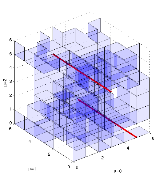
which is analogous (and equivalent, see (25)) to the average plaquette. We measure values like for example at and at . In Fig. 1 we visualize a typical graph occurring in the simulation, larger systems look even more cluttered. Histograms counting the frequencies of separations are accumulated after each individual PS step and turn out to be rather flat, as expected in the critical theory, where the Polyakov correlation decays only slowly.
During each iteration of A2nr we separately accumulate contributions to observables from the subset of vacuum configurations encountered during this iteration, like for example for . In the end we perform an autocorrelation analysis of this time series to estimate errors as described in [24]. The such defined integrated autocorrelation time of is shown in Fig. 2.
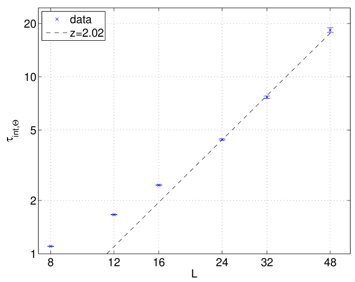
It is in units of A2nr iterations which cost proportional to . We see that while the absolute values are not too large on our lattices the rate of growth exhibits critical slowing down with an effective dynamical exponent for our range of lattice sizes close to two. Note that we cannot make statements on the truly asymptotic dynamical exponent on the basis of these data.
Of greater interest than are the topological observables (18). Taking into account the symmetries between all planes we here measure the set of observables
| (47) |
Due to (24) each can be simply related to ratios of partition functions with twisted and untwisted boundary conditions and is hence expected to possess finite continuum or scaling limits. In particular, at the exact critical point there are definite finite values for each in the limit at . In fact, this property may be used to determine . Note that the values are not independent, of course, but have to sum to unity. Our raw results on these quantities are compiled in Table 3 in the Appendix. We here consider the expected finite size scaling behavior close to the critical point in the form
| (48) |
where is the exponent of the leading scaling violations. In our simulations at we find the results shown in Fig. 3. In the variable a linear approach to is thus expected. Recent determinations of the exponent can be found in [22] and [25] - we use .
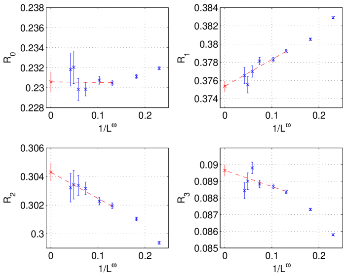
We show simple fits for our lattices with . Details on raw data are given in the appendix. We here just list the extrapolated values , , , .
4.2 Simulations in the confined phase
In the confined phase we simulate with algorithm A1, such that the distribution of has a direct relation to the temporal Polyakov loop correlator (29). We do not generate surfaces wrapping around the 12 plane corresponding to dynamically summing over twisted and untwisted boundary conditions for this plane. The Polyakov correlator is however periodic in space in this situation.
For our test we took the coupling with and a series of inverse temperatures Such values (but smaller ) have been adopted in [17] and a string tension in lattice units of has been estimated based on earlier literature. In our simulations in the confined phase we want to use a in (27) that essentially captures the decay of the two point function (29). Inspired by the lowest term in (35) we prepare777 The sum is singular for . We replace it by an extrapolation along the diagonal solving .
| (49) |
The mass is estimated from by using the first three terms on the right hand side of . The sum over integer , which makes periodic, is actually truncated after a few terms as the remainder would be insignificant compared to roundoff due to the exponential decay of the Bessel function. We emphasize that any imperfection in is related to the efficiency of the simulations but does not entail any systematic error.
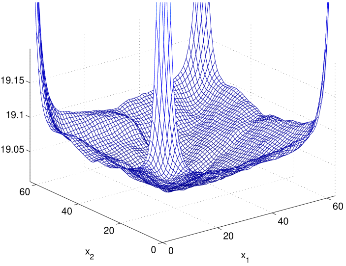
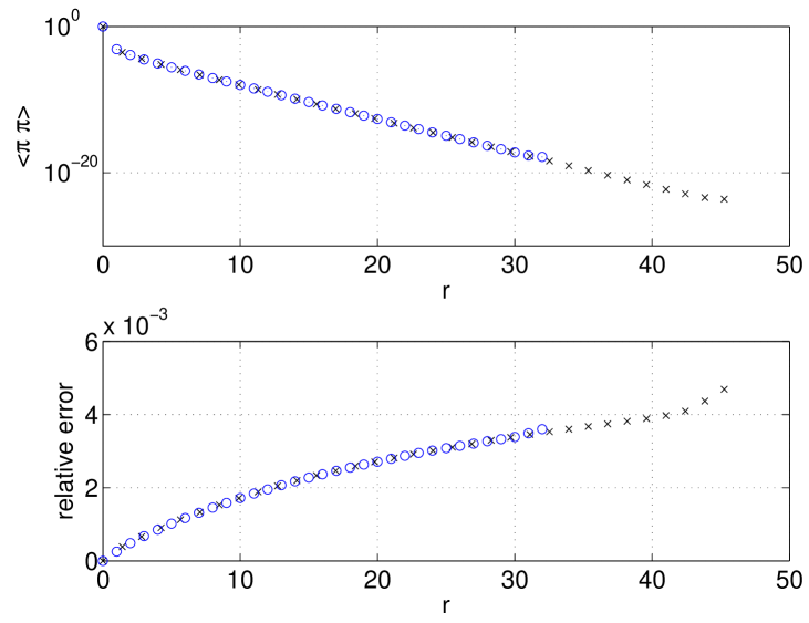
For each value of we have performed iterations of A1. In Fig. 4 we show the histogram of the frequencies of sampled separations of the two defect lines in our run for . With the exception of very short torus distances we find a rather flat behavior (note the fine scale of this logarithmic plot) which leads to very uniform bin heights, which, up to correlation effects, would naively imply constant relative errors. Via (29) this allows to measure the correlator which for the same run is plotted in Fig. 5. To determine errors here, we had to store the time series for these separations rather than just the histogram. We see that the exponential decay can be followed over the whole lattice with relative errors staying small. The plot jointly exhibits ‘on axis’ and ‘diagonal’ separations which form a very smooth curve and thus exhibit small violations of rotation invariance. The spatial correlation length is of order one and therefore the periodicity is just barely visible close to and .
| 6 | 0.160286(15) | 0.165454(28) | 18 | 0.762774(77) | 0.104107(89) |
| 8 | 0.279241(21) | 0.138969(31) | 20 | 0.853968(98) | 0.10092(12) |
| 10 | 0.384096(28) | 0.126905(37) | 22 | 0.94450(12) | 0.09807(13) |
| 12 | 0.482528(36) | 0.118760(45) | 24 | 1.03480(14) | 0.09571(15) |
| 14 | 0.577660(47) | 0.112776(55) | 26 | 1.12416(16) | 0.09329(18) |
| 16 | 0.670782(60) | 0.108026(60) | 28 | 1.21429(19) | 0.09154(21) |
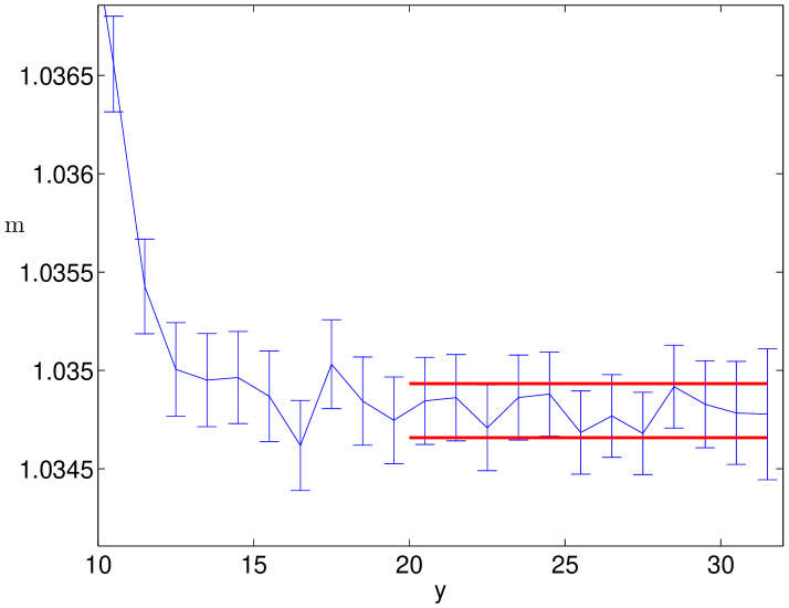
The closed string mass gap is estimated from (36) and our rather precise results are compiled in Table 1. A typical case of the determination of the mass gap is shown in Fig. 6. Effective masses are determined by solving . The horizontal lines show the error band from a fit deeply in the plateau region which leads to the entries for in the table. Observed autocorrelation times for these derived quantities [24] range from 0.508(4) ( to 0.598(6) (. The remarkable feature here is, that the errors in the effective masses do not grow with separation. This is due to our judicious adaptation of the simulated ensemble by choosing . The situation is analogous to the one in the Ising spin model [2] where the reasons for this success are discussed in more detail.
What is the implication of our fluctuating boundary conditions in the 12 plane for the correlation (36)? The falloff in the direction is associated with the transfer matrix in this direction which acts on wave-‘functionals’ . The Polyakov operator (28) acts on them by multiplication. The integration over links in the Euclidean theory implies the inclusion of a projector on gauge invariant states in the thermal trace given by the path ‘integral’. This refers to gauge transformations that are periodic in both directions. One may however in addition consider transformations [18] that are topologically nontrivial, here antiperiodic in , and physical states may be even or odd under them. By summing over twisted and untwisted boundary conditions in the 12 plane we include a projector also with respect to this quantum number. Under the assumption that the ground state is even, such a projection is no disadvantage.
To analyze our data we perform a fit of the form
| (50) |
To have visible errors at all we immediately plot the difference between the left and right hand side of such a fit against in Fig. 7. The fit here was derived from the subset of the data. The point with is much higher while is far off the panel. At these time extents the low temperature expansion has clearly and rather abruptly broken down. In fact, for our the phase transition is close to according to [17].
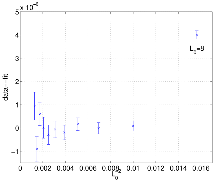
We note that (50) is exactly equivalent to the Nambu Goto form (32) if we identify
| (51) |
In Table 2 we list a number of fits (50) with free together with the resulting ratio for whose error the correlation between and is taken into account.
| 10 | 8.0/8 | 1.0109(13) | 0.0440330(25) | 0.046363(35) |
|---|---|---|---|---|
| 12 | 8.0/7 | 1.0114(23) | 0.0440334(32) | 0.046374(62) |
| 14 | 8.0/6 | 1.0111(40) | 0.0440332(42) | 0.04637(11) |
We see a small but significant deviation of from one by only about 1%. The most likely explanation for this are cut off effects in our opinion, given that the string tension in lattice units, which may be taken as indicative for their size, is about . It remains to be discussed to which terms in the expansion (33) our fits are actually sensitive. The errors of our are 7%, 24% , 68% of the last term in (33) for . The analogous numbers for the next term are 50%, 236%, 897%. This next term reads and this is only taken as a model of conceivable next order terms. We thus have to conclude that in spite of our rather high precision we are just still sensitive to the last (known) universal term of order and cannot confirm or disprove the coefficient of here.
In future simulations it will be desirable to simulate smaller lattice spacings to check the size of cutoff effects and possibly to enlarge the statistics to the point of seriously probing another term in (34).
5 Conclusions
We have attempted to generalize the worm algorithm for the Ising model to gauge theories with Ising link variables. The labeling of all-order (in ) strong coupling graphs as configurations of constrained plaquette fields was straight forward. The essential method of [1] to achieve efficient updates of the graphs was to allow for a pair of point defects. The possible defects in the gauge case form a very large set of generalized loop networks. We could not identify among them a suitable subset that strongly reduces critical slowing down while staying ‘close to’ the vacuum or simple Wilson loop defects.
The defects in the spin model allowed at the same time for a very precise estimation of the fundamental correlation at large distance [2]. We successfully have generalized this aspect to the gauge model and could compute the Polyakov line correlator with similar precision. At the same time, the algorithmic efficiency is rather high on large lattices in three dimensions in spite of critical slowing down.
Other Abelian gauge theories have been considered in the surface representation, see for example [7], [9], [10]. The techniques for correlators in this paper can clearly be generalized to these cases, i.e. to the groups Z() or U(1). Theories with SU() variables, both gauge and the principal chiral spin models888 Note that while there is mention of worm simulations of SU(3) spin models in the literature [26], their nontrivial symmetry is Z(3). are open problems in this context to which we hope to come back in the future.
Acknowledgments: UW is indebted to many people for helpful discussions: Tim Garoni, Martin Hasenbusch, Stefano Lottini, Mike Peardon, Stefan Sint, Erhard Seiler, Rainer Sommer and Peter Weisz. Financial support of the DFG via SFB transregio 9 is acknowledged.
Appendix
In this appendix we list the raw data on which Fig. 3 is based. Each line represents iterations of algorithm A2nr as described in subsection 3.4 except for where the number has been doubled. The error of these quantities seems to grow roughly proportionally to with a fixed number of iterations whose costs scale like .
| 6 | 0.23194(15) | 0.38290(10) | 0.29937(11) | 0.08579(6) |
|---|---|---|---|---|
| 8 | 0.23112(19) | 0.38053(13) | 0.30103(13) | 0.08731(7) |
| 12 | 0.23047(29) | 0.37920(18) | 0.30196(19) | 0.08838(10) |
| 16 | 0.23075(40) | 0.37828(25) | 0.30227(26) | 0.08870(14) |
| 24 | 0.22985(68) | 0.37813(41) | 0.30317(44) | 0.08884(23) |
| 32 | 0.22983(110) | 0.37699(62) | 0.30338(69) | 0.08980(35) |
| 40 | 0.23204(163) | 0.37553(90) | 0.30343(100) | 0.08901(50) |
| 48 | 0.23182(165) | 0.37653(89) | 0.30321(100) | 0.08844(48) |
References
- [1] N. Prokof’ev and B. Svistunov, Worm Algorithms for Classical Statistical Models, Phys. Rev. Lett. 87 (2001) 160601, [arXiv:0910.1393].
- [2] U. Wolff, Simulating the All-Order Strong Coupling Expansion I: Ising Model Demo, Nucl. Phys. B810 (2009) 491, [arXiv:0808.3934].
- [3] H. A. Kramers and G. H. Wannier, Statistics of the Two-Dimensional Ferromagnet. Part I, Phys. Rev. 60 (Aug, 1941) 252–262.
- [4] U. Wolff, Strong coupling expansion Monte Carlo, PoS LATTICE2010 (2010) [arXiv:1009.0657].
- [5] Q. Liu, Y. Deng, and T. M. Garoni, Worm Monte Carlo study of the honeycomb-lattice loop model, Nucl.Phys. B846 (2011) 283–315, [arXiv:1011.1980].
- [6] Q.-Q. Liu, Y. Deng, T. M. Garoni, and H. W. Blöte, The O(n) loop model on a three-dimensional lattice, Nucl.Phys. B859 (2012) 107–128, [arXiv:1112.5647].
- [7] M. G. Endres, Method for simulating O(N) lattice models at finite density, Phys.Rev. D75 (2007) 065012, [hep-lat/0610029].
- [8] V. Azcoiti, E. Follana, A. Vaquero, and G. Di Carlo, Geometric Algorithm for Abelian-Gauge Models, JHEP 0908 (2009) 008, [arXiv:0905.0639].
- [9] T. Korzec and U. Wolff, A worm-inspired algorithm for the simulation of Abelian gauge theories, PoS LATTICE2010 (2010) [arXiv:1011.1359].
- [10] C. Gattringer and A. Schmidt, Gauge and matter fields as surfaces and loops - an exploratory lattice study of the Z(3) Gauge-Higgs model, Phys.Rev. D86 (2012) 094506, [arXiv:1208.6472].
- [11] Y. Delgado, C. Gattringer, and A. Schmidt, Surface worm algorithm for abelian Gauge-Higgs systems on the lattice, arXiv:1211.3436.
- [12] M. Lüscher and P. Weisz, Quark confinement and the bosonic string, JHEP 0207 (2002) 049, [hep-lat/0207003].
- [13] M. Lüscher and P. Weisz, String excitation energies in SU(N) gauge theories beyond the free-string approximation, JHEP 0407 (2004) 014, [hep-th/0406205].
- [14] O. Aharony and E. Karzbrun, On the effective action of confining strings, JHEP 0906 (2009) 012, [arXiv:0903.1927].
- [15] M. Caselle and P. Grinza, On the intrinsic width of the chromoelectric flux tube in finite temperature LGTs, JHEP 1211 (2012) 174, [arXiv:1207.6523].
- [16] M. Billo, M. Caselle, and R. Pellegrini, New numerical results and novel effective string predictions for Wilson loops, JHEP 1201 (2012) 104, [arXiv:1107.4356].
- [17] M. Caselle, M. Hasenbusch, and M. Panero, String effects in the 3-d gauge Ising model, JHEP 0301 (2003) 057, [hep-lat/0211012].
- [18] G. ’t Hooft, A Property of Electric and Magnetic Flux in Nonabelian Gauge Theories, Nucl.Phys. B153 (1979) 141.
- [19] M. Hogervorst and U. Wolff, Finite size scaling and triviality of theory on an antiperiodic torus, Nucl.Phys. B855 (2012) 885–900, [arXiv:1109.6186].
- [20] J. Arvis, The exact q anti-q potential in Nambu string theory, Phys.Lett. B127 (1983) 106.
- [21] T. Sterling and J. Greensite, Portraits of the flux tube in QED in three-dimensions: A Monte Carlo Simulation with external sources, Nucl.Phys. B220 (1983) 327.
- [22] Y. Deng and H. W. Blöte, Simultaneous analysis of several models in the three-dimensional Ising universality class, Phys.Rev. E68 (2003) 036125.
- [23] M. Hasenbusch, Thermodynamic Casimir effect: Universality and Corrections to Scaling, Phys.Rev. B85 (2012) 174421, [arXiv:1202.6206].
- [24] ALPHA Collaboration, U. Wolff, Monte Carlo Errors with less Errors, Comput. Phys. Commun. 156 (2004) 143, [hep-lat/0306017].
- [25] M. Hasenbusch, A Finite Size Scaling Study of Lattice Models in the 3D Ising Universality Class, Phys.Rev. B82 (2010) 174433, [arXiv:1004.4486].
- [26] Y. D. Mercado and C. Gattringer, Monte Carlo simulation of the SU(3) spin model with chemical potential in a flux representation, Nucl.Phys. B862 (2012) 737–750, [arXiv:1204.6074].