Layer-wise training of deep generative models

Abstract

When using deep, multi-layered architectures to build generative models of data, it is difficult to train all layers at once. We propose a layer-wise training procedure admitting a performance guarantee compared to the global optimum. It is based on an optimistic proxy of future performance, the best latent marginal. We interpret auto-encoders in this setting as generative models, by showing that they train a lower bound of this criterion. We test the new learning procedure against a state of the art method (stacked RBMs), and find it to improve performance. Both theory and experiments highlight the importance, when training deep architectures, of using an inference model (from data to hidden variables) richer than the generative model (from hidden variables to data).

Introduction

Deep architectures, such as multiple-layer neural networks, have recently been the object of a lot of interest and have been shown to provide state-of-the-art performance on many problems [3]. A key aspect of deep learning is to help in learning better representations of the data, thus reducing the need for hand-crafted features, a very time-consuming process requiring expert knowledge.

Due to the difficulty of training a whole deep network at once, a so-called layer-wise procedure is used as an approximation [12, 1]. However, a long-standing issue is the justification of this layer-wise training: although the method has shown its merits in practice, theoretical justifications fall somewhat short of expectations. A frequently cited result [12] is a proof that adding layers increases a so-called variational lower bound on the log-likelihood of the model, and therefore that adding layers can improve performance.

We reflect on the validity of layer-wise training procedures, and discuss in what way and with what assumptions they can be construed as being equivalent to the non-layer-wise, that is, whole-network, training. This leads us to a new approach for training deep generative models, using a new criterion for optimizing each layer starting from the bottom and for transferring the problem upwards to the next layer. Under the right conditions, this new layer-wise approach is equivalent to optimizing the log-likelihood of the full deep generative model (Theorem 1).

As a first step, in Section 1 we re-introduce the general form of deep generative models, and derive the gradient of the log-likelihood for deep models. This gradient is seldom ever considered because it is considered intractable and requires sampling from complex distributions. Hence the need for a simpler, layer-wise training procedure.

We then show (Section 2.1) how an optimistic criterion, the BLM upper bound, can be used to train optimal lower layers provided subsequent training of upper layers is successful, and discuss what criterion to use to transfer the learning problem to the upper layers.

This leads to a discussion of the relation of this procedure with stacked restricted Boltzmann machines (SRBMs) and auto-encoders (Sections 2.3 and 2.4), in which a new justification is found for auto-encoders as optimizing the lower part of a deep generative model.

In Section 2.7 we spell out the theoretical advantages of using a model for the hidden variable $\mathbf{h}$ having the form $Q(\mathbf{h})=q(\mathbf{h}|\mathbf{x})P_{\mathrm{data}}(\mathbf{x})$ when looking for hidden-variable generative models of the data $\mathbf{x}$, a scheme close to that of auto-encoders.

Finally, we discuss new applications and perform experiments (Section 3) to validate the approach and compare it to state-of-the-art methods, on two new deep datasets, one synthetic and one real. In particular we introduce auto-encoders with rich inference (AERIes) which are auto-encoders modified according to this framework.

Indeed both theory and experiments strongly suggest that, when using stacked auto-associators or similar deep architectures, the inference part (from data to latent variables) should use a much richer model than the generative part (from latent variables to data), in fact, as rich as possible. Using richer inference helps to find much better parameters for the same given generative model.

1 Deep generative models

Let us go back to the basic formulation of training a deep architecture as a traditional learning problem: optimizing the parameters of the whole architecture seen as a probabilistic generative model of the data.

1.1 Deep models: probability decomposition

The goal of generative learning is to estimate the parameters $\theta=(\theta_{1},\dots,\theta_{n})$ of a distribution $P_{\theta}(\mathbf{x})$ in order to approximate a data distribution $P_{\mathcal{D}}(\mathbf{x})$ on some observed variable $\mathbf{x}$.

The recent development of deep architectures [12, 1] has given importance to a particular case of latent variable models in which the distribution of $\mathbf{x}$ can be decomposed as a sum over states of latent variables $\mathbf{h}$,

$$P_{\theta}(\mathbf{x})=\sum_{\mathbf{h}}P_{\theta_{1},\dots,\theta_{k}}(\mathbf{x}|\mathbf{h})P_{\theta_{k+1},\dots,\theta_{n}}(\mathbf{h})$$

with separate parameters for the marginal probability of $\mathbf{h}$ and the conditional probability of $\mathbf{x}$ given $\mathbf{h}$. Setting $I=\{1,2,\dots,k\}$ such that $\theta_{I}$ is the set of parameters of $P(\mathbf{x}|\mathbf{h})$ and $J=\{k+1,\dots,n\}$ such that $\theta_{J}$ is the set of parameters of $P(\mathbf{h})$, this rewrites as

$$P_{\theta}(\mathbf{x}) = \sum_{\mathbf{h}}P_{\theta_{I}}(\mathbf{x}|\mathbf{h})P_{\theta_{J}}(\mathbf{h})$$ (1)

In deep architectures, the same kind of decomposition is applied to $\mathbf{h}$ itself recursively, thus defining a layered model with several hidden layers $\mathbf{h}^{(1)}$, $\mathbf{h}^{(2)}$, …, $\mathbf{h}^{(k_{\mathrm{max}})}$, namely

$$P_{\theta}(\mathbf{x}) = \sum_{\mathbf{h}^{(1)}}P_{\theta_{I_{0}}}(\mathbf{x}|\mathbf{h}^{(1)})P_{\theta_{J_{0}}}(\mathbf{h}^{(1)})$$ (2)

$$P(\mathbf{h}^{(k)}) = \sum_{\mathbf{h}^{(k+1)}}P_{\theta_{I_{k}}}(\mathbf{h}^{(k)}|\mathbf{h}^{(k+1)})P_{\theta_{J_{k}}}(\mathbf{h}^{(k+1)}),\,\,\,1\leqslant k\leqslant k_{\mathrm{max}}-1$$ (3)

At any one time, we will only be interested in one step of this decomposition. Thus for simplicity, we consider that the distribution of interest is on the observed variable $\mathbf{x}$, with latent variable $\mathbf{h}$. The results extend to the other layers of the decomposition by renaming variables.

In Sections 2.3 and 2.4 we quickly present two frequently used deep architectures, stacked RBMs and auto-encoders, within this framework.

1.2 Data log-likelihood

The goal of the learning procedure, for a probabilistic generative model, is generally to maximize the log-likelihood of the data under the model, namely, to find the value of the parameter $\theta^{*}=(\theta_{I}^{*},\theta_{J}^{*})$ achieving

$$\theta^{*} \mathrel{\mathop{:}}= \operatorname*{arg\,max}_{\theta}\mathbb{E}_{\mathbf{x}\sim P_{\mathcal{D}}}\left[\log P_{\theta}(\mathbf{x})\right]$$ (4)

$$= \operatorname*{arg\,min}_{\theta}D_{\mathrm{KL}}(P_{\mathcal{D}}\!\parallel\!P_{\theta}),$$ (5)

where $P_{\mathcal{D}}$ is the empirical data distribution, and $D_{\mathrm{KL}}(\cdot\!\parallel\!\cdot)$ is the Kullback–Leibler divergence. (For simplicity we assume this optimum is unique.)

An obvious way to tackle this problem would be a gradient ascent over the full parameter $\theta$. However, this is impractical for deep architectures (Section 1.3 below).

It would be easier to be able to train deep architectures in a layer-wise fashion, by first training the parameters $\theta_{I}$ of the bottom layer, deriving a new target distribution for the latent variables $\mathbf{h}$, and then training $\theta_{J}$ to reproduce this target distribution on $\mathbf{h}$, recursively over the layers, till one reaches the top layer on which, hopefully, a simple probabilistic generative model can be used.

Indeed this is often done in practice, except that the objective (4) is replaced with a surrogate objective. For instance, for architectures made of stacked RBMs, at each level the likelihood of a single RBM is maximized, ignoring the fact that it is to be used as part of a deep architecture, and moreover often using a further approximation to the likelihood such as contrastive divergence [11]. Under specific conditions (i.e., initializing the upper layer with an upside-down version of the current RBM), it can be shown that adding a layer improves a lower bound on performance [12].

We address in Section 2 the following questions: Is it possible to compute or estimate the optimal value of the parameters $\theta^{\ast}_{I}$ of the bottom layer, without training the whole model? Is it possible to compare two values of $\theta_{I}$ without training the whole model? The latter would be particularly convenient for hyper-parameter selection, as it would allow to compare lower-layer models before the upper layers are trained, thus significantly reducing the size of the hyper-parameter search space from exponential to linear in the number of layers.

We propose a procedure aimed at reaching the global optimum $\theta^{\ast}$ in a layer-wise fashion, based on an optimistic estimate of log-likelihood, the best latent marginal (BLM) upper bound. We study its theoretical guarantees in Section 2. In Section 3 we make an experimental comparison between stacked RBMs, auto-encoders modified according to this scheme, and vanilla auto-encoders, on two simple but deep datasets.

1.3 Learning by gradient ascent for deep architectures

Maximizing the likelihood of the data distribution $P_{\mathcal{D}}(\mathbf{x})$ under a model, or equivalently minimizing the KL-divergence $D_{\mathrm{KL}}(P_{\mathcal{D}}\!\parallel\!P_{\theta})$, is usually done with gradient ascent in the parameter space.

The derivative of the log-likelihood for a deep generative model can be written as:

$$\frac{\partial\log P_{\mathbf{\theta}}(\mathbf{x})}{\partial\theta} = \frac{\sum_{\mathbf{h}}\frac{\partial P_{\theta_{I}}(\mathbf{x}|\mathbf{h})}{\partial\theta}P_{\theta_{J}}(\mathbf{h})+\sum_{\mathbf{h}}P_{\theta_{I}}(\mathbf{x}|\mathbf{h})\frac{\partial P_{\theta_{J}}(\mathbf{h})}{\partial\theta}}{P_{\theta}(\mathbf{x})}$$ (6)

$$= \sum_{\mathbf{h}}\frac{\partial\log P_{\theta_{I}}(\mathbf{x}|\mathbf{h})}{\partial\theta}P_{\theta}(\mathbf{h}|\mathbf{x})+\sum_{\mathbf{h}}\frac{\partial\log P_{\theta_{J}}(\mathbf{h})}{\partial\theta}P_{\theta}(\mathbf{h}|\mathbf{x})$$ (7)

by rewriting $P_{\theta}(\mathbf{h})/P_{\theta}(\mathbf{x})=P_{\theta}(\mathbf{h}|\mathbf{x})/P_{\theta}(\mathbf{x}|\mathbf{h})$. The derivative w.r.t. a given component $\theta_{i}$ of $\theta$ simplifies because $\theta_{i}$ is either a parameter of $P_{\theta_{I}}(\mathbf{x}|\mathbf{h})$ when $i\in I$, or a parameter of $P_{\theta_{J}}(\mathbf{h})$ when $i\in J$:

$$\forall i\in I,\qquad \frac{\partial\log P_{\mathbf{\theta}}(\mathbf{x})}{\partial\theta_{i}}=\sum_{\mathbf{h}}\frac{\partial\log P_{\theta_{I}}(\mathbf{x}|\mathbf{h})}{\partial\theta_{i}}P_{\theta_{I},\theta_{J}}(\mathbf{h}|\mathbf{x}),$$ (8)

$$\forall i\in J,\qquad \frac{\partial\log P_{\mathbf{\theta}}(\mathbf{x})}{\partial\theta_{i}}=\sum_{\mathbf{h}}\frac{\partial\log P_{\theta_{J}}(\mathbf{h})}{\partial\theta_{i}}P_{\theta_{I},\theta_{J}}(\mathbf{h}|\mathbf{x}).$$ (9)

Unfortunately, this gradient ascent procedure is generally intractable, because it requires sampling from $P_{\theta_{I},\theta_{J}}(\mathbf{h}|\mathbf{x})$ (where both the upper layer and lower layer influence $\mathbf{h}$) to perform inference in the deep model.

2 Layer-wise deep learning

2.1 A theoretical guarantee

We now present a training procedure that works successively on each layer. First we train $\theta_{I}$ together with a conditional model $q(\mathbf{h}|\mathbf{x})$ for the latent variable knowing the data. This step involves only the bottom part of the model and is thus often tractable. This allows to infer a new target distribution for $\mathbf{h}$, on which the upper layers can then be trained.

This procedure singles out a particular setting $\hat{\theta}_{I}$ for the bottom layer of a deep architecture, based on an optimistic assumption of what the upper layers may be able to do (cf. Proposition 3).

Under this procedure, Theorem 1 states that it is possible to obtain a validation that the parameter $\hat{\theta}_{I}$ for the bottom layer was optimal, provided the rest of the training goes well. Namely, if the target distribution for $\mathbf{h}$ can be realized or well approximated by some value of the parameters $\theta_{J}$ of the top layers, and if $\theta_{I}$ was obtained using a rich enough conditional model $q(\mathbf{h}|\mathbf{x})$, then $(\theta_{I},\theta_{J})$ is guaranteed to be globally optimal.

Theorem 1.

Suppose the parameters $\theta_{I}$ of the bottom layer are trained by

$$(\hat{\theta}_{I},\hat{q})\mathrel{\mathop{:}}=\operatorname*{arg\,max}_{\theta_{I},q}\mathbb{E}_{\mathbf{x}\sim P_{\mathcal{D}}}\left[\log\sum_{\mathbf{h}}P_{\theta_{I}}(\mathbf{x}|\mathbf{h})\,q_{\mathcal{D}}(\mathbf{h})\right]$$ (10)

where the arg max runs over all conditional probability distributions $q(\mathbf{h}|\mathbf{x})$ and where

$$q_{\mathcal{D}}(\mathbf{h})\mathrel{\mathop{:}}=\sum_{\tilde{\mathbf{x}}}q(\mathbf{h}|\tilde{\mathbf{x}})P_{\mathcal{D}}(\tilde{\mathbf{x}})$$ (11)

with $P_{\mathcal{D}}$ the observed data distribution.

We call the optimal $\hat{\theta}_{I}$ the best optimistic lower layer (BOLL). Let $\hat{q}_{\mathcal{D}}(\mathbf{h})$ be the distribution on $\mathbf{h}$ associated with the optimal $\hat{q}$. Then:

• If the top layers can be trained to reproduce $\hat{q}_{\mathcal{D}}(\mathbf{h})$ perfectly, i.e., if there exists a parameter $\hat{\theta}_{J}$ for the top layers such that the distribution $P_{\hat{\theta}_{J}}(\mathbf{h})$ is equal to $\hat{q}_{\mathcal{D}}(\mathbf{h})$, then the parameters obtained are globally optimal:

  $$(\hat{\theta}_{I},\hat{\theta}_{J})=(\theta_{I}^{\ast},\theta_{J}^{\ast})$$

• Whatever parameter value $\theta_{J}$ is used on the top layers in conjunction with the BOLL $\hat{\theta}_{I}$, the difference in performance (4) between $(\hat{\theta}_{I},\theta_{J})$ and the global optimum $(\theta_{I}^{\ast},\theta_{J}^{\ast})$ is at most the Kullback–Leibler divergence $D_{\mathrm{KL}}(\hat{q}_{\mathcal{D}}(\mathbf{h})\!\parallel\!P_{\theta_{J}}(\mathbf{h}))$ between $\hat{q}_{\mathcal{D}}(\mathbf{h})$ and $P_{\theta_{J}}(\mathbf{h})$.

This theorem strongly suggests using $\hat{q}_{\mathcal{D}}(\mathbf{h})$ as the target distribution for the top layers, i.e., looking for the value $\hat{\theta}_{J}$ best approximating $\hat{q}_{\mathcal{D}}(\mathbf{h})$:

$$\hat{\theta}_{J}\mathrel{\mathop{:}}=\operatorname*{arg\,min}_{\theta_{J}}D_{\mathrm{KL}}(\hat{q}_{\mathcal{D}}(\mathbf{h})\!\parallel\!P_{\theta_{J}}(\mathbf{h}))=\operatorname*{arg\,max}_{\theta_{J}}\mathbb{E}_{\mathbf{h}\sim\hat{q}_{\mathcal{D}}}\log P_{\theta_{J}}(\mathbf{h})$$ (12)

which thus takes the same form as the original problem. Then the same scheme may be used recursively to train the top layers. A final fine-tuning phase may be helpful, see Section 2.6.

Note that when the top layers fail to approximate $\hat{q}_{\mathcal{D}}$ perfectly, the loss of performance depends only on the observed difference between $\hat{q}_{\mathcal{D}}$ and $P_{\hat{\theta}_{J}}$, and not on the unknown global optimum $(\theta_{I}^{\ast},\theta_{J}^{\ast})$. Beware that, unfortunately, this bound relies on perfect layer-wise training of the bottom layer, i.e., on $\hat{q}$ being the optimum of the criterion (10) optimized over all possible conditional distributions $q$; otherwise it is a priori not valid.

In practice the supremum on $q$ will always be taken over a restricted set of conditional distributions $q(\mathbf{h}|\mathbf{x})$, rather than the set of all possible distributions on $\mathbf{h}$ for each $\mathbf{x}$. Thus, this theorem is an idealized version of practice (though Remark 4 below mitigates this). This still suggests a clear strategy to separate the deep optimization problem into two subproblems to be solved sequentially:

1. Train the parameters $\theta_{I}$ of the bottom layer after (10), using a model $q(\mathbf{h}|\mathbf{x})$ as wide as possible, to approximate the BOLL $\hat{\theta}_{I}$.

2. Infer the corresponding distribution of $\mathbf{h}$ by (11) and train the upper part of the model as best as possible to approximate this distribution.

Then, provided learning is successful in both instances, the result is close to optimal.

Auto-encoders can be shown to implement an approximation of this procedure, in which only the terms $\mathbf{x}=\tilde{\mathbf{x}}$ are kept in (10)–(11) (Section 2.4).

This scheme is designed with in mind a situation in which the upper layers get progessively simpler. Indeed, if the layer for $\mathbf{h}$ is as wide as the layer for $\mathbf{x}$ and if $P(\mathbf{x}|\mathbf{h})$ can learn the identity, then the procedure in Theorem 1 just transfers the problem unchanged one layer up.

This theorem strongly suggests decoupling the inference and generative models $q(\mathbf{h}|\mathbf{x})$ and $P(\mathbf{x}|\mathbf{h})$, and using a rich conditional model $q(\mathbf{h}|\mathbf{x})$, contrary, e.g., to common practice in auto-encoders. Indeed the experiments of Section 3 confirm that using a more expressive $q(\mathbf{h}|\mathbf{x})$ yields improved values of $\theta$.

Importantly, $q(\mathbf{h}|\mathbf{x})$ is only used as an auxiliary prop for solving the optimization problem (4) over $\theta$ and is not part of the final generative model, so that using a richer $q(\mathbf{h}|\mathbf{x})$ to reach a better value of $\theta$ is not simply changing to a larger model. Thus, using a richer inference model $q(\mathbf{h}|\mathbf{x})$ should not pose too much risk of overfitting because the regularization properties of the model come mainly from the choice of the generative model family $(\theta)$.

The criterion proposed in (10) is of particular relevance to representation learning where the goal is not to learn a generative model, but to learn a useful representation of the data. In this setting, training an upper layer model $P(\mathbf{h})$ becomes irrelevant because we are not interested in the generative model itself. What matters in representation learning is that the lower layer (i.e., $P(\mathbf{x}|\mathbf{h})$ and $q(\mathbf{h}|\mathbf{x})$) is optimal for some model of $P(\mathbf{h})$, left unspecified.

We now proceed, by steps, to the proof of Theorem 1. This will be the occasion to introduce some concepts used later in the experimental setting.

2.2 The Best Latent Marginal Upper Bound

One way to evaluate a parameter $\theta_{I}$ for the bottom layer without training the whole architecture is to be optimistic: assume that the top layers will be able to produce the probability distribution for $\mathbf{h}$ that gives the best results if used together with $P_{\theta_{I}}(\mathbf{x}|\mathbf{h})$. This leads to the following.

Definition 2.

Let $\theta_{I}$ be a value of the bottom layer parameters. The best latent marginal (BLM) for $\theta_{I}$ is the probability distribution $Q$ on $\mathbf{h}$ maximizing the log-likelihood:

$$\hat{Q}_{\theta_{I},\mathcal{D}}\mathrel{\mathop{:}}=\operatorname*{arg\,max}_{Q}\mathbb{E}_{\mathbf{x}\sim P_{\mathcal{D}}}\left[\log\sum_{\mathbf{h}}P_{\theta_{I}}(\mathbf{x}|\mathbf{h})Q(\mathbf{h})\right]$$ (13)

where the arg max runs over the set of all probability distributions over $\mathbf{h}$. The BLM upper bound is the corresponding log-likelihood value:

$$\mathcal{U}_{\mathcal{D}}(\theta_{I})\mathrel{\mathop{:}}=\max_{Q}\mathbb{E}_{\mathbf{x}\sim P_{\mathcal{D}}}\left[\log\sum_{\mathbf{h}}P_{\theta_{I}}(\mathbf{x}|\mathbf{h})Q(\mathbf{h})\right]$$ (14)

The BLM upper bound $\mathcal{U}_{\mathcal{D}}(\theta_{I})$ is the least upper bound on the log-likelihood of the deep generative model on the dataset $\mathcal{D}$ if $\theta_{I}$ is used for the bottom layer. $\mathcal{U}_{\mathcal{D}}(\theta_{I})$ is only an upper bound of the actual performance of $\theta_{I}$, because subsequent training of $P_{\theta_{J}}(\mathbf{h})$ may be suboptimal: the best latent marginal $\hat{Q}_{\theta_{I},\mathcal{D}}(\mathbf{h})$ may not be representable as $P_{\theta_{J}}(\mathbf{h})$ for $\theta_{J}$ in the model, or the training of $P_{\theta_{J}}(\mathbf{h})$ itself may not converge to the best solution.

Note that the arg max in (13) is concave in $Q$, so that in typical situations the BLM is unique—except in degenerate cases such as when two values of $\mathbf{h}$ define the same $P_{\theta_{I}}(\mathbf{x}|\mathbf{h})$).

Proposition 3.

The criterion (10) used in Theorem 1 for training the bottom layer coincides with the BLM upper bound:

$$\mathcal{U}_{\mathcal{D}}(\theta_{I})=\max_{q}\mathbb{E}_{\mathbf{x}\sim P_{\mathcal{D}}}\left[\log\sum_{\mathbf{h}}P_{\theta_{I}}(\mathbf{x}|\mathbf{h})q_{\mathcal{D}}(\mathbf{h})\right]$$ (15)

where the maximum runs over all conditional probability distributions $q(\mathbf{h}|\mathbf{x})$. In particular the BOLL $\hat{\theta}_{I}$ selected in Theorem 1 is

$$\hat{\theta}_{I}=\operatorname*{arg\,max}_{\theta_{I}}\,\mathcal{U}_{\mathcal{D}}(\theta_{I})$$ (16)

and the target distribution $\hat{q}_{\mathcal{D}}(\mathbf{h})$ in Theorem 1 is the best latent marginal $\hat{Q}_{\hat{\theta}_{I},\mathcal{D}}$.

Thus the BOLL $\hat{\theta}_{I}$ is the best bottom layer setting if one uses an optimistic criterion for assessing the bottom layer, hence the name “best optimistic lower layer”.

Proof.

Any distribution $Q$ over $\mathbf{h}$ can be written as $q_{\mathcal{D}}$ for some conditional distribution $q(\mathbf{h}|\mathbf{x})$, for instance by defining $q(\mathbf{h}|\mathbf{x})=Q(\mathbf{h})$ for every $\mathbf{x}$ in the dataset. In particular this is the case for the best latent marginal $\hat{Q}_{\theta_{I},\mathcal{D}}$.

Consequently the maxima in (15) and in (14) are taken on the same set and coincide. ∎

The argument that any distribution is of the form $q_{\mathcal{D}}$ may look disappointing: why choose this particular form? In Section 2.7 we show how writing distributions over $\mathbf{h}$ as $q_{\mathcal{D}}$ for some conditional distribution $q(\mathbf{h}|\mathbf{x})$ may help to maximize data log-likelihood, by quantifiably incorporating information from the data (Proposition 7). Moreover, the bound on loss of performance (second part of Theorem 1) when the upper layers do not match the BLM crucially relies on the properties of $\hat{q}_{\mathcal{D}}$. A more practical argument for using $q_{\mathcal{D}}$ is that optimizing both $\theta_{I}$ and the full distribution of the hidden variable $\mathbf{h}$ at the same time is just as difficult as optimizing the whole network, whereas the deep architectures currently in use already train a model of $\mathbf{x}$ knowing $\mathbf{h}$ and of $\mathbf{h}$ knowing $\mathbf{x}$ at the same time.

Remark 4.

For Theorem 1 to hold, it is not necessary to optimize over all possible conditional probability distributions $q(\mathbf{h}|\mathbf{x})$ (which is a set of very large dimension). As can be seen from the proof above it is enough to optimize over a family $q(\mathbf{h}|\mathbf{x})\in\mathcal{Q}$ such that every (non-conditional) distribution on $\mathbf{h}$ can be represented (or well approximated) as $q_{\mathcal{D}}(\mathbf{h})$ for some $q\in\mathcal{Q}$.

Let us now go on with the proof of Theorem 1.

Proposition 5.

Set the bottom layer parameters to the BOLL

$$\hat{\theta}_{I} =\operatorname*{arg\,max}_{\theta_{I}}\,\mathcal{U}_{\mathcal{D}}(\theta_{I})$$ (17)

and let $\hat{Q}$ be the corresponding best latent marginal.

Assume that subsequent training of the top layers using $\hat{Q}$ as the target distribution for $\mathbf{h}$, is successful, i.e., there exists a $\theta_{J}$ such that $\hat{Q}(\mathbf{h})=P_{\theta_{J}}(\mathbf{h})$.

Then $\hat{\theta}_{I}=\theta_{I}^{\ast}$.

Proof.

Define the in-model BLM upper bound as

$$\mathcal{U}^{\mathrm{model}}_{\mathcal{D}}(\theta_{I})\mathrel{\mathop{:}}=\max_{\theta_{J}}\mathbb{E}_{\mathbf{x}\sim P_{\mathcal{D}}}\left[\log\sum_{\mathbf{h}}P_{\theta_{I}}(\mathbf{x}|\mathbf{h})P_{\theta_{J}}(\mathbf{h})\right]$$ (18)

By definition, the global optimum $\theta_{I}^{\ast}$ for the parameters of the whole architecture is given by $\theta_{I}^{\ast}=\operatorname*{arg\,max}_{\theta_{I}}\mathcal{U}^{\mathrm{model}}_{\mathcal{D}}(\theta_{I})$.

Obviously, for any value $\theta_{I}$ we have $\mathcal{U}^{\mathrm{model}}_{\mathcal{D}}(\theta_{I})\leqslant\mathcal{U}_{\mathcal{D}}(\theta_{I})$ since the argmax is taken over a more restricted set. Then, in turn, $\mathcal{U}_{\mathcal{D}}(\theta_{I})\leqslant\mathcal{U}_{\mathcal{D}}(\hat{\theta}_{I})$ by definition of $\hat{\theta}_{I}$.

By our assumption, the BLM $\hat{Q}$ for $\hat{\theta}_{I}$ happens to lie in the model: $\hat{Q}(\mathbf{h})=P_{\theta_{J}}(\mathbf{h})$. This implies that $\mathcal{U}_{\mathcal{D}}(\hat{\theta}_{I})=\mathcal{U}^{\mathrm{model}}_{\mathcal{D}}(\hat{\theta}_{I})$.

Combining, we get that $\mathcal{U}^{\mathrm{model}}_{\mathcal{D}}(\theta_{I})\leqslant\mathcal{U}^{\mathrm{model}}_{\mathcal{D}}(\hat{\theta}_{I})$ for any $\theta_{I}$. Thus $\hat{\theta}_{I}$ maximizes $\mathcal{U}^{\mathrm{model}}_{\mathcal{D}}(\theta_{I})$, and is thus equal to $\theta_{I}^{\ast}$. ∎

The first part of Theorem 1 then results from the combination of Propositions 5 and 3.

We now give a bound on the loss of performance in case further training of the upper layers fails to reproduce the BLM. This will complete the proof of Theorem 1. We will make use of a special optimality property of distributions of the form $q_{\mathcal{D}}(\mathbf{h})$, namely, Proposition 7, whose proof is postponed to Section 2.7.

Proposition 6.

Keep the notation of Theorem 1. In the case when $P_{\theta_{J}}(\mathbf{h})$ fails to reproduce $\hat{q}_{\mathcal{D}}(\mathbf{h})$ exactly, the loss of performance of $(\hat{\theta}_{I},\theta_{J})$ with respect to the global optimum $(\theta^{\ast}_{I},\theta^{\ast}_{J})$ is at most

$$D_{\mathrm{KL}}(P_{\mathcal{D}}(\mathbf{x})\!\parallel\!P_{\hat{\theta}_{I},\theta_{J}}(\mathbf{x}))-D_{\mathrm{KL}}(P_{\mathcal{D}}(\mathbf{x})\!\parallel\!\hat{q}_{\mathcal{D},\hat{\theta}_{I}}(\mathbf{x}))$$ (19)

where $\hat{q}_{\mathcal{D},\hat{\theta}_{I}}(\mathbf{x})\mathrel{\mathop{:}}=\sum_{\mathbf{h}}P_{\hat{\theta}_{I}}(\mathbf{x}|\mathbf{h})\hat{q}_{\mathcal{D}}(\mathbf{h})$ is the distribution on $\mathbf{x}$ obtained by using the BLM.

This quantity is in turn at most

$$D_{\mathrm{KL}}(\hat{q}_{\mathcal{D}}(\mathbf{h})\!\parallel\!P_{\theta_{J}}(\mathbf{h}))$$ (20)

which is thus also a bound on the loss of performance of $(\hat{\theta}_{I},\theta_{J})$ with respect to $(\theta^{\ast}_{I},\theta^{\ast}_{J})$.

Note that these estimates do not depend on the unkown global optimum $\theta^{*}$.

Importantly, this bound is not valid if $\hat{q}$ has not been perfectly optimized over all possible conditional distributions $q(\mathbf{h}|\mathbf{x})$. Thus it should not be used blindly to get a performance bound, since heuristics will always be used to find $\hat{q}$. Therefore, it may have only limited practical relevance. In practice the real loss may both be larger than this bound because $q$ has been optimized over a smaller set, and smaller because we are comparing to the BLM upper bound which is an optimistic assessment.

Proof.

From (4) and (5), the difference in log-likelihood performance between any two distributions $p_{1}(\mathbf{x})$ and $p_{2}(\mathbf{x})$ is equal to $D_{\mathrm{KL}}(P_{\mathcal{D}}\!\parallel\!p_{1})-D_{\mathrm{KL}}(P_{\mathcal{D}}\!\parallel\!p_{2})$.

For simplicity, denote

$$p_{1}(\mathbf{x}) =P_{\hat{\theta}_{I},\theta_{J}}(\mathbf{x})=\sum_{\mathbf{h}}P_{\hat{\theta}_{I}}(\mathbf{x}|\mathbf{h})P_{\theta_{J}}(\mathbf{h})$$

$$p_{2}(\mathbf{x}) =P_{\theta_{I}^{\ast},\theta_{J}^{\ast}}(\mathbf{x})=\sum_{\mathbf{h}}P_{\theta_{I}^{\ast}}(\mathbf{x}|\mathbf{h})P_{\theta_{J}^{\ast}}(\mathbf{h})$$

$$p_{3}(\mathbf{x}) =\sum_{\mathbf{h}}P_{\hat{\theta}_{I}}(\mathbf{x}|\mathbf{h})\hat{q}_{\mathcal{D}}(\mathbf{h})$$

We want to compare $p_{1}$ and $p_{2}$.

Define the in-model upper bound $\mathcal{U}^{\mathrm{model}}_{\mathcal{D}}(\theta_{I})$ as in (18) above. Then we have $\theta_{I}^{\ast}=\operatorname*{arg\,max}_{\theta_{I}}\mathcal{U}^{\mathrm{model}}_{\mathcal{D}}(\theta_{I})$ and $\hat{\theta}_{I}=\operatorname*{arg\,max}_{\theta_{I}}\mathcal{U}_{\mathcal{D}}(\theta_{I})$. Since $\mathcal{U}^{\mathrm{model}}_{\mathcal{D}}\leqslant\mathcal{U}_{\mathcal{D}}$, we have $\mathcal{U}^{\mathrm{model}}_{\mathcal{D}}(\theta_{I}^{\ast})\leqslant\mathcal{U}_{D}(\hat{\theta}_{I})$. The BLM upper bound $\mathcal{U}_{D}(\hat{\theta}_{I})$ is attained when we use $\hat{q}_{\mathcal{D}}$ as the distribution for $\mathbf{h}$, so $\mathcal{U}^{\mathrm{model}}_{\mathcal{D}}(\theta_{I}^{\ast})\leqslant\mathcal{U}_{D}(\hat{\theta}_{I})$ means that the performance of $p_{3}$ is better than the performance of $p_{2}$:

$$D_{\mathrm{KL}}(P_{\mathcal{D}}\!\parallel\!p_{3})\leqslant D_{\mathrm{KL}}(P_{\mathcal{D}}\!\parallel\!p_{2})$$

(inequalities hold in the reverse order for data log-likelihood).

Now by definition of the optimum $\theta^{\ast}$, the distribution $p_{2}$ is better than $p_{1}$: $D_{\mathrm{KL}}(P_{\mathcal{D}}\!\parallel\!p_{2})\leqslant D_{\mathrm{KL}}(P_{\mathcal{D}}\!\parallel\!p_{1})$. Consequently, the difference in performance between $p_{2}$ and $p_{1}$ (whether expressed in data log-likelihood or in Kullback–Leibler divergence) is smaller than the difference in performance between $p_{3}$ and $p_{1}$, which is the difference of Kullback–Leibler divergences appearing in the proposition.

Let us now evaluate more precisely the loss of $p_{1}$ with respect to $p_{3}$. By abuse of notation we will indifferently denote $p_{1}(\mathbf{h})$ and $p_{1}(\mathbf{x})$, it being understood that one is obtained from the other through $P_{\hat{\theta}_{I}}(\mathbf{x}|\mathbf{h})$, and likewise for $p_{3}$ (with the same $\hat{\theta}_{I}$).

For any distributions $p_{1}$ and $p_{3}$ the loss of performance of $p_{1}$ w.r.t. $p_{3}$ satisfies

$$\mathbb{E}_{\mathbf{x}\sim P_{\mathcal{D}}}\log p_{3}(\mathbf{x})-\mathbb{E}_{\mathbf{x}\sim P_{\mathcal{D}}}\log p_{1}(\mathbf{x})=\mathbb{E}_{\mathbf{x}\sim P_{\mathcal{D}}}\left[\log\frac{\sum_{\mathbf{h}}P_{\hat{\theta}_{I}}(\mathbf{x}|\mathbf{h})p_{3}(\mathbf{h})}{\sum_{\mathbf{h}}P_{\hat{\theta}_{I}}(\mathbf{x}|\mathbf{h})p_{1}(\mathbf{h})}\right]$$

and by the log sum inequality $\log(\sum a_{i}/\sum b_{i})\leqslant\frac{1}{\sum a_{i}}\sum a_{i}\log(a_{i}/b_{i})$ [9, Theorem 2.7.1] we get

$$\mathbb{E}_{\mathbf{x}\sim P_{\mathcal{D}}}\log p_{3}(\mathbf{x})-\mathbb{E}_{\mathbf{x}\sim P_{\mathcal{D}}}\log p_{1}(\mathbf{x})$$

$$\leqslant\mathbb{E}_{\mathbf{x}\sim P_{\mathcal{D}}}\left[\frac{1}{\sum_{\mathbf{h}}P_{\hat{\theta}_{I}}(\mathbf{x}|\mathbf{h})p_{3}(\mathbf{h})}\sum_{\mathbf{h}}P_{\hat{\theta}_{I}}(\mathbf{x}|\mathbf{h})p_{3}(\mathbf{h})\log\frac{P_{\hat{\theta}_{I}}(\mathbf{x}|\mathbf{h})p_{3}(\mathbf{h})}{P_{\hat{\theta}_{I}}(\mathbf{x}|\mathbf{h})p_{1}(\mathbf{h})}\right]$$

$$=\mathbb{E}_{\mathbf{x}\sim P_{\mathcal{D}}}\left[\frac{1}{p_{3}(\mathbf{x})}\sum_{\mathbf{h}}p_{3}(\mathbf{x},\mathbf{h})\log\frac{p_{3}(\mathbf{h})}{p_{1}(\mathbf{h})}\right]$$

$$=\mathbb{E}_{\mathbf{x}\sim P_{\mathcal{D}}}\left[\sum_{\mathbf{h}}p_{3}(\mathbf{h}|\mathbf{x})\log\frac{p_{3}(\mathbf{h})}{p_{1}(\mathbf{h})}\right]$$

$$=\mathbb{E}_{\mathbf{x}\sim P_{\mathcal{D}}}\mathbb{E}_{\mathbf{h}\sim p_{3}(\mathbf{h}|\mathbf{x})}\left[\log\frac{p_{3}(\mathbf{h})}{p_{1}(\mathbf{h})}\right]$$

Given a probability $p_{3}$ on $(\mathbf{x},\mathbf{h})$, the law on $\mathbf{h}$ obtained by taking an $\mathbf{x}$ according to $P_{\mathcal{D}}$, then taking an $\mathbf{h}$ according to $p_{3}(\mathbf{h}|\mathbf{x})$, is generally not equal to $p_{3}(\mathbf{h})$. However, here $p_{3}$ is equal to the BLM $\hat{q}_{D}$, and by Proposition 7 below the BLM has exactly this property (which characterizes the log-likelihood extrema). Thus thanks to Proposition 7 we have

$$\mathbb{E}_{\mathbf{x}\sim P_{\mathcal{D}}}\mathbb{E}_{\mathbf{h}\sim\hat{q}_{\mathcal{D}}(\mathbf{h}|\mathbf{x})}\left[\log\frac{\hat{q}_{\mathcal{D}}(\mathbf{h})}{p_{1}(\mathbf{h})}\right]=\mathbb{E}_{\mathbf{h}\sim\hat{q}_{\mathcal{D}}}\left[\log\frac{\hat{q}_{\mathcal{D}}(\mathbf{h})}{p_{1}(\mathbf{h})}\right]=D_{\mathrm{KL}}(\hat{q}_{\mathcal{D}}(\mathbf{h})\!\parallel\!p_{1}(\mathbf{h}))$$

which concludes the argument. ∎

2.3 Relation with Stacked RBMs

Stacked RBMs (SRBMs) [12, 1, 14] are deep generative models trained by stacking restricted Boltzmann machines (RBMs) [23].

A RBM uses a single set of parameters to represent a distribution on pairs $(\mathbf{x},\mathbf{h})$. Similarly to our approach, stacked RBMs are trained in a greedy layer-wise fashion: one starts by training the distribution of the bottom RBM to approximate the distribution of $\mathbf{x}$. To do so, distributions $P_{\theta_{I}}(\mathbf{x}|\mathbf{h})$ and $Q_{\theta_{I}}(\mathbf{h}|\mathbf{x})$ are learned jointly using a single set of parameters $\theta_{I}$. Then a target distribution for $\mathbf{h}$ is defined as $\sum_{\mathbf{x}}Q_{\theta_{I}}(\mathbf{h}|\mathbf{x})P_{\mathcal{D}}(\mathbf{x})$ (similarly to (11)) and the top layers are trained recursively on this distribution.

In the final generative model, the full top RBM is used on the top layer to provide a distribution for $\mathbf{h}$, then the bottom RBMs are used only for the generation of $\mathbf{x}$ knowing $\mathbf{h}$. (Therefore the $\mathbf{h}$-biases of the bottom RBMs are never used in the final generative model.)

Thus, in contrast with our approach, $P_{\theta_{I}}(\mathbf{x}|\mathbf{h})$ and $Q_{\theta_{I}}(\mathbf{h}|\mathbf{x})$ are not trained to maximize the least upper bound of the likelihood of the full deep generative model but are trained to maximize the likelihood of a single RBM.

This procedure has been shown to be equivalent to maximizing the likelihood of a deep generative model with infinitely many layers where the weights are all tied [12]. The latter can be interpreted as an assumption on the future value of $P(\mathbf{h})$, which is unknown when learning the first layer. As such, SRBMs make a different assumption about the future $P(\mathbf{h})$ than the one made in (10).

With respect to this, the comparison of gradient ascents is instructive: the gradient ascent for training the bottom RBM takes a form reminiscent of gradient ascent of the global generative model (7) but in which the dependency of $P(\mathbf{h})$ on the upper layers $\theta_{J}$ is ignored, and instead the distribution $P(\mathbf{h})$ is tied to $\theta_{I}$ because the RBM uses a single parameter set for both.

When adding a new layer on top of a trained RBM, if the initialization is set to an upside down version of the current RBM (which can be seen as “unrolling” one step of Gibbs sampling), the new deep model still matches the special infinite deep generative model with tied weights mentioned above. Starting training of the upper layer from this initialization guarantees that the new layer can only increase the likelihood [12]. However, this result is only known to hold for two layers; with more layers, it is only known that adding layers increases a bound on the likelihood [12].

In our approach, the perspective is different. During the training of lower layers, we consider the best possible model for the hidden variable. Because of errors which are bound to occur in approximation and optimization during the training of the model for $P(\mathbf{h})$, the likelihood associated with an optimal upper model (the BLM upper bound) is expected to decrease each time we actually take another lower layer into account: At each new layer, errors in approximation or optimization occur so that the final likelihood of the training set will be smaller than the upper bound. (On the other way these limitations might actually improve performance on a test set, see the discussion about regularization in Section 3.)

In [16] a training criterion is suggested for SRBMs which is reminiscent of a BLM with tied weights for the inference and generative parts (and therefore without the BLM optimality guarantee), see also Section 2.5.

2.4 Relation with Auto-Encoders

Since the introduction of deep neural networks, auto-encoders [24] have been considered a credible alternative to stacked RBMs and have been shown to have almost identical performance on several tasks [15].

Auto-encoders are trained by stacking auto-associators [7] trained with backpropagation. Namely: we start with a three-layer network $\mathbf{x}\mapsto\mathbf{h}^{(1)}\mapsto\mathbf{x}$ trained by backpropagation to reproduce the data; this provides two conditional distributions $P(\mathbf{h}^{(1)}|\mathbf{x})$ and $P(\mathbf{x}|\mathbf{h}^{(1)})$. Then in turn, another auto-associator is trained as a three-layer network $\mathbf{h}^{(1)}\mapsto\mathbf{h}^{(2)}\mapsto\mathbf{h}^{(1)}$, to reproduce the distribution $P(\mathbf{h}^{(1)}|\mathbf{x})$ on $\mathbf{h}^{(1)}$, etc.

So as in the learning of SRBMs, auto-encoder training is performed in a greedy layer-wise manner, but with a different criterion: the reconstruction error.

Note that after the auto-encoder has been trained, the deep generative model is incomplete because it lacks a generative model for the distribution $P(\mathbf{h}^{k_{\mathrm{max}}})$ of the deepest hidden variable, which the auto-encoder does not provide. One possibility is to learn the top layer with an RBM, which then completes the generative model.

Concerning the theoretical soundness of stacking auto-associators for training deep generative models, it is known that the training of auto-associators is an approximation of the training of RBMs in which only the largest term of an expansion of the log-likelihood is kept [4]. In this sense, SRBM and stacked auto-associator training approximate each other (see also Section 2.5).

Our approach gives a new understanding of auto-encoders as the lower part of a deep generative model, because they are trained to maximize a lower bound of (10), as follows.

To fix ideas, let us consider for (10) a particular class of conditional distributions $q(\mathbf{h}|\mathbf{x})$ commonly used in auto-associators. Namely, let us parametrize $q$ as $q_{\xi}$ with

$$q_{\xi}(\mathbf{h}|\mathbf{x}) = \prod_{j}q_{\xi}(h_{j}|\mathbf{x})$$ (21)

$$q_{\xi}(h_{j}|\mathbf{x}) = \operatorname{sigm}({\textstyle\sum}_{i}x_{i}w_{ij}+b_{j})$$ (22)

where the parameter vector is $\xi=\{\mathbf{W},\mathbf{b}\}$ and $\operatorname{sigm}(\cdot)$ is the sigmoid function.

Given a conditional distribution $q(\mathbf{h}|\mathbf{x})$ as in Theorem 1, let us expand the distribution on $\mathbf{x}$ obtained from $P_{\theta_{I}}(\mathbf{x}|\mathbf{h})$ and $q_{\mathcal{D}}(\mathbf{h})$:

$$P(\mathbf{x}) =\sum_{\mathbf{h}}P_{\theta_{I}}(\mathbf{x}|\mathbf{h})q_{\mathcal{D}}(\mathbf{h})$$ (23)

$$=\sum_{\mathbf{h}}P_{\theta_{I}}(\mathbf{x}|\mathbf{h})\sum_{\tilde{\mathbf{x}}}q(\mathbf{h}|\tilde{\mathbf{x}})P_{\mathcal{D}}(\tilde{\mathbf{x}})$$ (24)

where as usual $P_{\mathcal{D}}$ is the data distribution. Keeping only the terms $\mathbf{x}=\tilde{\mathbf{x}}$ in this expression we see that

$$P(\mathbf{x})\geqslant\sum_{\mathbf{h}}P_{\theta_{I}}(\mathbf{x}|\mathbf{h})q(\mathbf{h}|\mathbf{x})P_{\mathcal{D}}(\mathbf{x})$$ (25)

Taking the sum of likelihoods over $\mathbf{x}$ in the dataset, this corresponds to the criterion maximized by auto-associators when they are considered from a probabilistic perspective. Since moreover optimizing over $q$ as in (10) is more general than optimizing over the particular class $q_{\xi}$, we conclude that the criterion optimized in auto-associators is a lower bound on the criterion (10) proposed in Theorem 1.

Keeping only $\mathbf{x}=\tilde{\mathbf{x}}$ is justified if we assume that inference is an approximation of the inverse of the generative process, that is, $P_{\theta_{I}}(\mathbf{x}|\mathbf{h})q(\mathbf{h}|\tilde{\mathbf{x}})\approx 0$ as soon as $\mathbf{x}\neq\tilde{\mathbf{x}}$. Thus under this assumption, both criteria will be close, so that Theorem 1 provides a justification for auto-encoder training in this case. On the other hand, this assumption can be strong: it implies that no $\mathbf{h}$ can be shared between different $\mathbf{x}$, so that for instance two observations cannot come from the same underlying latent variable through a random choice. Depending on the situation this might be unrealistic. Still, using this as a training criterion might perform well even if the assumption is not fully satisfied.

Note that we chose the form of $q_{\xi}(\mathbf{h}|\mathbf{x})$ to match that of the usual auto-associator, but of course we could have made a different choice such as using a multilayer network for $q_{\xi}(\mathbf{h}|\mathbf{x})$ or $P_{\theta_{I}}(\mathbf{x}|\mathbf{h})$. These possibilities will be explored later in this article.

2.5 From stacked RBMs to auto-encoders: layer-wise consistency

We now show how imposing a “layer-wise consistency” constraint on stacked RBM training leads to the training criterion used in auto-encoders with tied weights. Some of the material here already appears in [16].

Let us call layer-wise consistent a layer-wise training procedure in which each layer determines a value $\theta_{I}$ for its parameters and a target distribution $P(\mathbf{h})$ for the upper layers which are mutually optimal in the following sense: if $P(\mathbf{h})$ is used a the distribution of the hidden variable, then $\theta_{I}$ is the bottom parameter value maximizing data log-likelihood.

The BLM training procedure is, by construction, layer-wise consistent.

Let us try to train stacked RBMs in a layer-wise consistent way. Given a parameter $\theta_{I}$, SRBMs use the hidden variable distribution

$$Q_{\mathcal{D},\theta_{I}}(\mathbf{h})=\mathbb{E}_{\mathbf{x}\sim P_{\mathcal{D}}}\,P_{\theta_{I}}(\mathbf{h}|\mathbf{x})$$ (26)

as the target for the next layer, where $P_{\theta_{I}}(\mathbf{h}|\mathbf{x})$ is the RBM distribution of $\mathbf{h}$ knowing $\mathbf{x}$. The value $\theta_{I}$ and this distribution over $\mathbf{h}$ are mutually optimal for each other if the distribution on $\mathbf{x}$ stemming from this distribution on $\mathbf{h}$, given by

$$P^{(1)}_{\theta_{I}}(\mathbf{x}) =\mathbb{E}_{\mathbf{h}\sim Q_{\mathcal{D},\theta_{I}}(\mathbf{h})}\,P_{\theta_{I}}(\mathbf{x}|\mathbf{h})$$ (27)

$$=\sum_{\mathbf{h}}P_{\theta_{I}}(\mathbf{x}|\mathbf{h})\sum_{\tilde{\mathbf{x}}}P_{\theta_{I}}(\mathbf{h}|\tilde{\mathbf{x}})P_{\mathcal{D}}(\tilde{\mathbf{x}})$$ (28)

maximizes log-likelihood, i.e.,

$$\theta_{I}=\operatorname*{arg\,min}D_{\mathrm{KL}}(P_{\mathcal{D}}(\mathbf{x})\!\parallel\!P^{(1)}_{\theta_{I}}(\mathbf{x}))$$ (29)

The distribution $P^{(1)}_{\theta_{I}}(\mathbf{x})$ is the one obtained from the data after one “forward-backward” step of Gibbs sampling $\mathbf{x}\to\mathbf{h}\to\mathbf{x}$ (cf. [16]).

But $P^{(1)}_{\theta_{I}}(\mathbf{x})$ is also equal to the distribution (24) for an auto-encoder with tied weights. So the layer-wise consistency criterion for RBMs coincides with tied-weights auto-encoder training, up to the approximation that in practice auto-encoders retain only the terms $\mathbf{x}=\tilde{\mathbf{x}}$ in the above (Section 2.4).

On the other hand, stacked RBM training trains the parameter $\theta_{I}$ to approximate the data distribution by the RBM distribution:

$$\theta^{\mathrm{RBM}}_{I}=\operatorname*{arg\,min}_{\theta_{I}}D_{\mathrm{KL}}(P_{\mathcal{D}}(\mathbf{x})\!\parallel\!P^{\mathrm{RBM}}_{\theta_{I}}(\mathbf{x}))$$ (30)

where $P^{\mathrm{RBM}}_{\theta_{I}}$ is the probability distribution of the RBM with parameter $\theta_{I}$, i.e. the probability distribution after an infinite number of Gibbs samplings from the data.

Thus, stacked RBM training and tied-weight auto-encoder training can be seen as two approximations to the layer-wise consistent optimization problem (29), one using the full RBM distribution $P^{\mathrm{RBM}}_{\theta_{I}}$ instead of $P^{(1)}_{\theta_{I}}$ and the other using $\mathbf{x}=\tilde{\mathbf{x}}$ in $P^{(1)}_{\theta_{I}}$.

It is not clear to us to which extent the criteria (29) using $P^{(1)}_{\theta_{I}}$ and $\eqref{eq:SRBMtraining}$ using $P^{\mathrm{RBM}}_{\theta_{I}}$ actually yield different values for the optimal $\theta_{I}$: although these two optimization criteria are different (unless RBM Gibbs sampling converges in one step), it might be that the optimal $\theta_{I}$ is the same (in which case SRBM training would be layer-wise consistent), though this seems unlikely.

The $\theta_{I}$ obtained from the layer-wise consistent criterion (29) using $P^{(1)}_{\theta_{I}}(\mathbf{x})$ will always perform at least as well as standard SRBM training if the upper layers match the target distribution on $\mathbf{h}$ perfectly—this follows from its very definition.

Nonetheless, it is not clear whether layer-wise consistency is always a desirable property. In SRBM training, replacing the RBM distribution over $\mathbf{h}$ with the one obtained from the data seemingly breaks layer-wise consistency, but at the same time it always improves data log-likelihood (as a consequence of Proposition 7 below).

For non-layer-wise consistent training procedures, fine-tuning of $\theta_{I}$ after more layers have been trained would improve performance. Layer-wise consistent procedures may require this as well in case the upper layers do not match the target distribution on $\mathbf{h}$ (while non-layer-wise consistent procedures would require this even with perfect upper layer training).

2.6 Relation to fine-tuning

When the approach presented in Section 2 is used recursively to train deep generative models with several layers using the criterion (10), irrecoverable losses may be incurred at each step: first, because the optimization problem (10) may be imperfectly solved, and, second, because each layer was trained using a BLM assumption about what upper layers are able to do, and subsequent upper layer training may not match the BLM. Consequently the parameters used for each layer may not be optimal with respect to each other. This suggests using a fine-tuning procedure.

In the case of auto-encoders, fine-tuning can be done by backpropagation on all (inference and generative) layers at once (Figure 1). This has been shown to improve performance in several contexts [14, 13], which confirms the expected gain in performance from recovering earlier approximation losses. In principle, there is no limit to the number of layers of an auto-encoder that could be trained at once by backpropagation, but in practice training many layers at once results in a difficult optimization problem with many local minima. Layer-wise training can be seen as a way of dealing with the issue of local minima, providing a solution close to a good optimum. This optimum is then reached by global fine-tuning.

Figure 1: Deep training with fine-tuning.

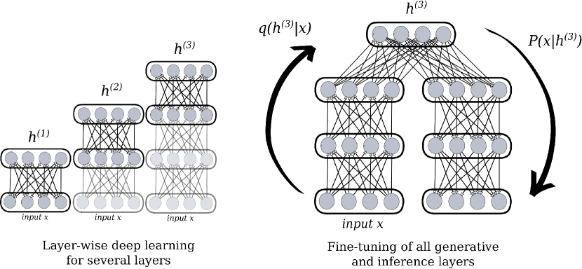
Fine-tuning can be described in the BLM framework as follows: fine-tuning is the maximization of the BLM upper bound (10) where all the layers are considered as one single complex layer (Figure 1). In the case of auto-encoders, the approximation $\mathbf{x}=\tilde{\mathbf{x}}$ in (10)–(11) is used to help optimization, as explained above.

Note that there is no reason to limit fine-tuning to the end of the layer-wise procedure: fine-tuning may be used at intermediate stages where any number of layers have been trained.

This fine-tuning procedure was not applied in the experiments below because our experiments only have one layer for the bottom part of the model.

As mentioned before, a generative model for the topmost hidden layer (e.g., an RBM) still needs to be trained to get a complete generative model after fine-tuning.

2.7 Data Incorporation: Properties of $q_{\mathcal{D}}$

It is not clear why it should be more interesting to work with the conditional distribution $q(\mathbf{h}|\mathbf{x})$ and then define a distribution on $\mathbf{h}$ through $q_{\mathcal{D}}$, rather than working directly with a distribution $Q$ on $\mathbf{h}$.

The first answer is practical: optimizing on $P_{\theta_{I}}(\mathbf{x}|\mathbf{h})$ and on the distribution of $\mathbf{h}$ simultaneously is just the same as optimizing over the global network, while on the other hand the currently used deep architectures provide both $\mathbf{x}|\mathbf{h}$ and $\mathbf{h}|\mathbf{x}$ at the same time.

A second answer is mathematical: $q_{\mathcal{D}}$ is defined through the dataset $\mathcal{D}$. Thus by working on $q(\mathbf{h}|\mathbf{x})$ we can concentrate on the correspondence between $\mathbf{h}$ and $\mathbf{x}$ and not on the full distribution of either, and hopefully this correspondence is easier to describe. Then we use the dataset $\mathcal{D}$ to provide $q_{\mathcal{D}}$: so rather than directly crafting a distribution $Q(\mathbf{h})$, we use a distribution which automatically incorporates aspects of the data distribution $\mathcal{D}$ even for very simple $q$. Hopefully this is better; we now formalize this argument.

Let us fix the bottom layer parameters $\theta_{I}$, and consider the problem of finding the best latent marginal over $\mathbf{h}$, i.e., the $Q$ maximizing the data log-likelihood

$$\operatorname*{arg\,max}_{Q}\mathbb{E}_{\mathbf{x}\sim P_{\mathcal{D}}}\left[\log\sum_{\mathbf{h}}P_{\theta_{I}}(\mathbf{x}|\mathbf{h})Q(\mathbf{h})\right]$$ (31)

Let $Q(\mathbf{h})$ be a candidate distribution. We might build a better one by “reflecting the data” in it. Namely, $Q(\mathbf{h})$ defines a distribution $P_{\theta_{I}}(\mathbf{x}|\mathbf{h})Q(\mathbf{h})$ on $(\mathbf{x},\mathbf{h})$. This distribution, in turn, defines a conditional distribution of $\mathbf{h}$ knowing $\mathbf{x}$ in the standard way:

$$Q^{\mathrm{cond}}(\mathbf{h}|\mathbf{x})\mathrel{\mathop{:}}=\frac{P_{\theta_{I}}(\mathbf{x}|\mathbf{h})Q(\mathbf{h})}{\sum_{\mathbf{h}^{\prime}}P_{\theta_{I}}(\mathbf{x}|\mathbf{h}^{\prime})Q(\mathbf{h}^{\prime})}$$ (32)

We can turn $Q^{\mathrm{cond}}(\mathbf{h}|\mathbf{x})$ into a new distribution on $\mathbf{h}$ by using the data distribution:

$$Q^{\mathrm{cond}}_{\mathcal{D}}(\mathbf{h})\mathrel{\mathop{:}}=\sum_{\mathbf{x}}Q^{\mathrm{cond}}(\mathbf{h}|\mathbf{x})P_{\mathcal{D}}(\mathbf{x})$$ (33)

and in general $Q^{\mathrm{cond}}_{\mathcal{D}}(\mathbf{h})$ will not coincide with the original distribution $Q(\mathbf{h})$, if only because the definition of the former involves the data whereas $Q$ is arbitrary. We will show that this operation is always an improvement: $Q^{\mathrm{cond}}_{\mathcal{D}}(\mathbf{h})$ always yields a better data log-likelihood than $Q$.

Proposition 7.

Let data incorporation be the map sending a distribution $Q(\mathbf{h})$ to $Q^{\mathrm{cond}}_{\mathcal{D}}(\mathbf{h})$ defined by (32) and (33), where $\theta_{I}$ is fixed. It has the following properties:

• Data incorporation always increases the data log-likelihood (31).

• The best latent marginal $\hat{Q}_{\theta_{I},\mathcal{D}}$ is a fixed point of this transformation. More precisely, the distributions $Q$ that are fixed points of data incorporation are exactly the critical points of the data log-likelihood (31) (by concavity of (31) these critical points are all maxima with the same value). In particular if the BLM is uniquely defined (the arg max in (13) is unique), then it is the only fixed point of data incorporation.

• Data incorporation $Q\mapsto Q^{\mathrm{cond}}_{\mathcal{D}}$ coincides with one step of the expectation-maximization (EM) algorithm to maximize data log-likelihood by optimizing over $Q$ for a fixed $\theta_{I}$, with $\mathbf{h}$ as the hidden variable.

This can be seen as a justification for constructing the hidden variable model $Q$ through an inference model $q(\mathbf{h}|\mathbf{x})$ from the data, which is the basic approach of auto-encoders and the BLM.

Proof.

Let us first prove the statement about expectation-maximization. Since the EM algorithm is known to increase data log-likelihood at each step [10, 25], this will prove the first statement as well.

For simplicity let us assume that the data distribution is uniform over the dataset $\mathcal{D}=(\mathbf{x}_{1},\ldots,\mathbf{x}_{n})$. (Arbitrary data weights can be approximated by putting the same observation several times into the data.) The hidden variable of the EM algorithm will be $\mathbf{h}$, and the parameter over which the EM optimizes will be the distribution $Q(\mathbf{h})$ itself. In particular we keep $\theta_{I}$ fixed. The distributions $Q$ and $P_{\theta_{I}}$ define a distribution $P(\mathbf{x},\mathbf{h})\mathrel{\mathop{:}}=P_{\theta_{I}}(\mathbf{x}|\mathbf{h})Q(\mathbf{h})$ over pairs $(\mathbf{x},\mathbf{h})$. This extends to a distribution over $n$-tuples of observations:

$$P((\mathbf{x}_{1},\mathbf{h}_{1}),\ldots,(\mathbf{x}_{n},\mathbf{h}_{n}))=\prod_{i}P_{\theta_{I}}(\mathbf{x}_{i}|\mathbf{h}_{i})Q(\mathbf{h}_{i})$$

and by summing over the states of the hidden variables

$$P(\mathbf{x}_{1},\ldots,\mathbf{x}_{n})=\sum_{(\mathbf{h}_{1},\ldots,\mathbf{h}_{n})}P((\mathbf{x}_{1},\mathbf{h}_{1}),\ldots,(\mathbf{x}_{n},\mathbf{h}_{n}))$$

Denote $\vec{\mathbf{x}}=(\mathbf{x}_{1},\ldots,\mathbf{x}_{n})$ and $\vec{\mathbf{h}}=(\mathbf{h}_{1},\ldots,\mathbf{h}_{n})$. One step of the EM algorithm operating with the distribution $Q$ as parameter, is defined as transforming the current distribution $Q_{t}$ into the new distribution

$$Q_{t+1}=\operatorname*{arg\,max}_{Q}\sum_{\vec{\mathbf{h}}}P_{t}(\vec{\mathbf{h}}|\vec{\mathbf{x}})\log P(\vec{\mathbf{x}},\vec{\mathbf{h}})$$

where $P_{t}(\vec{\mathbf{x}},\vec{\mathbf{h}})=P_{\theta_{I}}(\vec{\mathbf{x}}|\vec{\mathbf{h}})Q_{t}(\vec{\mathbf{h}})$ is the distribution obtained by using $Q_{t}$ for $\mathbf{h}$, and $P$ the one obtained from the distribution $Q$ over which we optimize. Let us follow a standard argument for EM algorithms on $n$-tuples of independent observations:

$$\sum_{\vec{\mathbf{h}}}P_{t}(\vec{\mathbf{h}}|\vec{\mathbf{x}})\log P(\vec{\mathbf{x}},\vec{\mathbf{h}}) =\sum_{\vec{\mathbf{h}}}P_{t}(\vec{\mathbf{h}}|\vec{\mathbf{x}})\log\prod_{i}P(\mathbf{x}_{i},\mathbf{h}_{i})$$

$$=\sum_{i}\sum_{\vec{\mathbf{h}}}P_{t}(\vec{\mathbf{h}}|\vec{\mathbf{x}})\log P(\mathbf{x}_{i},\mathbf{h}_{i})$$

Since observations are independent, $P_{t}(\vec{\mathbf{h}}|\vec{\mathbf{x}})$ decomposes as a product and so

$$\sum_{i}\sum_{\vec{\mathbf{h}}}(\log P(\mathbf{x}_{i},\mathbf{h}_{i}))P_{t}(\vec{\mathbf{h}}|\vec{\mathbf{x}}) =\sum_{i}\sum_{\mathbf{h}_{1},\ldots,\mathbf{h}_{n}}(\log P(\mathbf{x}_{i},\mathbf{h}_{i}))\prod_{j}P_{t}(\mathbf{h}_{j}|\mathbf{x}_{j})$$

$$=\sum_{i}\sum_{\mathbf{h}_{i}}(\log P(\mathbf{x}_{i},\mathbf{h}_{i}))P_{t}(\mathbf{h}_{i}|\mathbf{x}_{i})\prod_{j\neq i}\sum_{\mathbf{h}_{j}}P_{t}(\mathbf{h}_{j}|\mathbf{x}_{j})$$

but of course $\sum_{\mathbf{h}_{j}}P_{t}(\mathbf{h}_{j}|\mathbf{x}_{j})=1$ so that finally

$$\sum_{\vec{\mathbf{h}}}P_{t}(\vec{\mathbf{h}}|\vec{\mathbf{x}})\log P(\vec{\mathbf{x}},\vec{\mathbf{h}}) =\sum_{i}\sum_{\mathbf{h}_{i}}(\log P(\mathbf{x}_{i},\mathbf{h}_{i}))P_{t}(\mathbf{h}_{i}|\mathbf{x}_{i})$$

$$=\sum_{\mathbf{h}}\sum_{i}(\log P(\mathbf{x}_{i},\mathbf{h}))P_{t}(\mathbf{h}|\mathbf{x}_{i})$$

$$=\sum_{\mathbf{h}}\sum_{i}(\log P_{\theta_{I}}(\mathbf{x}_{i}|\mathbf{h})+\log Q(\mathbf{h}))P_{t}(\mathbf{h}|\mathbf{x}_{i})$$

because $P(\mathbf{x},\mathbf{h})=P_{\theta_{I}}(\mathbf{x}|\mathbf{h})Q(\mathbf{h})$. We have to maximize this quantity over $Q$. The first term does not depend on $Q$ so we only have to maximize $\sum_{\mathbf{h}}\sum_{i}(\log Q(\mathbf{h}))P_{t}(\mathbf{h}|\mathbf{x}_{i})$.

This latter quantity is concave in $Q$, so to find the maximum it is sufficient to exhibit a point where the derivative w.r.t. $Q$ (subject to the constraint that $Q$ is a probability distribution) vanishes.

Let us compute this derivative. If we replace $Q$ with $Q+\delta Q$ where $\delta Q$ is infinitesimal, the variation of the quantity to be maximized is

$$\sum_{\mathbf{h}}\sum_{i}(\delta\log Q(\mathbf{h}))P_{t}(\mathbf{h}|\mathbf{x}_{i})=\sum_{\mathbf{h}}\frac{\delta Q(\mathbf{h})}{Q(\mathbf{h})}\sum_{i}P_{t}(\mathbf{h}|\mathbf{x}_{i})$$

Let us take $Q=(Q_{t})^{\mathrm{cond}}_{\mathcal{D}}$. Since we assumed for simplicity that the data distribution $\mathcal{D}$ is uniform over the sample this $(Q_{t})^{\mathrm{cond}}_{\mathcal{D}}$ is

$$Q(\mathbf{h})=(Q_{t})^{\mathrm{cond}}_{\mathcal{D}}(\mathbf{h})=\frac{1}{n}\sum_{i}P_{t}(\mathbf{h}|\mathbf{x}_{i})$$

so that the variation of the quantity to be maximized is

$$\sum_{\mathbf{h}}\frac{\delta Q(\mathbf{h})}{Q(\mathbf{h})}\sum_{i}P_{t}(\mathbf{h}|\mathbf{x}_{i})=n\sum_{\mathbf{h}}\delta Q(\mathbf{h})$$

But since $Q$ and $Q+\delta Q$ are both probability distributions, both sum to $1$ over $\mathbf{h}$ so that $\sum_{\mathbf{h}}\delta Q(\mathbf{h})=0$. This proves that this choice of $Q$ is an extremum of the quantity to be maximized.

This proves the last statement of the proposition. As mentioned above, it implies the first by the general properties of EM. Once the first statement is proven, the best latent marginal $\hat{Q}_{\theta_{I},\mathcal{D}}$ has to be a fixed point of data incorporation, because otherwise we would get an even better distribution thus contradicting the definition of the BLM.

The only point left to prove is the equivalence between critical points of the log-likelihood and fixed points of $Q\mapsto Q^{\mathrm{cond}}_{\mathcal{D}}$. This is a simple instance of maximization under constraints, as follows. Critical points of the data log-likelihood are those for which the log-likelihood does not change at first order when $Q$ is replaced with $Q+\delta Q$ for small $\delta Q$. The only constraint on $\delta Q$ is that $Q+\delta Q$ must still be a probability distribution, so that $\sum_{\mathbf{h}}\delta Q(\mathbf{h})=0$ because both $Q$ and $Q+\delta Q$ sum to $1$.

The first-order variation of log-likelihood is

$$\delta\sum_{i}\log P(\mathbf{x}_{i}) =\delta\sum_{i}\log\left(\sum_{\mathbf{h}}P_{\theta_{I}}(\mathbf{x}_{i}|\mathbf{h})Q(\mathbf{h})\right)$$

$$=\sum_{i}\frac{\delta\sum_{\mathbf{h}}P_{\theta_{I}}(\mathbf{x}_{i}|\mathbf{h})Q(\mathbf{h})}{\sum_{\mathbf{h}}P_{\theta_{I}}(\mathbf{x}_{i},\mathbf{h})Q(\mathbf{h})}$$

$$=\sum_{i}\frac{\sum_{\mathbf{h}}P_{\theta_{I}}(\mathbf{x}_{i}|\mathbf{h})\delta Q(\mathbf{h})}{P(\mathbf{x}_{i})}$$

$$=\sum_{\mathbf{h}}\delta Q(\mathbf{h})\sum_{i}\frac{P_{\theta_{I}}(\mathbf{x}_{i}|\mathbf{h})}{P(\mathbf{x}_{i})}$$

$$=\sum_{\mathbf{h}}\delta Q(\mathbf{h})\sum_{i}\frac{P(\mathbf{x}_{i},\mathbf{h})/Q(\mathbf{h})}{P(\mathbf{x}_{i})}$$

$$=\sum_{\mathbf{h}}\delta Q(\mathbf{h})\sum_{i}\frac{P(\mathbf{h}|\mathbf{x}_{i})}{Q(\mathbf{h})}$$

This must vanish for any $\delta Q$ such that $\sum_{\mathbf{h}}\delta Q(\mathbf{h})=0$. By elementary linear algebra (or Lagrange multipliers) this occurs if and only if $\sum_{i}\frac{P(\mathbf{h}|\mathbf{x}_{i})}{Q(\mathbf{h})}$ does not depend on $\mathbf{h}$, i.e., if and only if $Q$ satisfies $Q(\mathbf{h})=C\sum_{i}P(\mathbf{h}|\mathbf{x}_{i})$. Since $Q$ sums to $1$ one finds $C=\frac{1}{n}$. Since all along $P$ is the probability distribution on $\mathbf{x}$ and $\mathbf{h}$ defined by $Q$ and $P_{\theta_{I}}(\mathbf{x}|\mathbf{h})$, namely, $P(\mathbf{x},\mathbf{h})=P_{\theta_{I}}(\mathbf{x}|\mathbf{h})Q(\mathbf{h})$, by definition we have $P(\mathbf{h}|\mathbf{x})=Q^{\mathrm{cond}}(\mathbf{h}|\mathbf{x})$ so that the condition $Q(\mathbf{h})=\frac{1}{n}\sum_{i}P(\mathbf{h}|\mathbf{x}_{i})$ exactly means that $Q=Q^{\mathrm{cond}}_{\mathcal{D}}$, hence the equivalence between critical points of log-likelihood and fixed points of data incorporation. ∎

3 Applications and Experiments

Given the approach described above, we now consider several applications for which we evaluate the method empirically.

The intractability of the log-likelihood for deep networks makes direct comparison of several methods difficult in general. Often the evaluation is done by using latent variables as features for a classification task and by direct visual comparison of samples generated by the model [14, 21]. Instead, we introduce two new datasets which are simple enough for the true log-likelihood to be computed explicitly, yet complex enough to be relevant to deep learning.

We first check that these two datasets are indeed deep.

Then we try to assess the impact of the various approximations from theory to practice, on the validity of the approach.

We then apply our method to the training of deep belief networks using properly modified auto-encoders, and show that the method outperforms current state of the art.

We also explore the use of the BLM upper bound to perform layer-wise hyper-parameter selection and show that it gives an accurate prediction of the future log-likelihood of models.

3.1 Low-Dimensional Deep Datasets

We now introduce two new deep datasets of low dimension. In order for those datasets to give a reasonable picture of what happens in the general case, we first have to make sure that they are relevant to deep learning, using the following approach:

1. In the spirit of [6], we train 1000 RBMs using CD-1 [11] on the dataset $\mathcal{D}$, and evaluate the log-likelihood of a disjoint validation dataset $\mathcal{V}$ under each model.

2. We train 1000 2-layer deep networks using stacked RBMs trained with CD-1 on $\mathcal{D}$, and evaluate the log-likelihood of $\mathcal{V}$ under each model.

3. We compare the performance of each model at equal number of parameters.

4. If deep networks consistently outperform single RBMs for the same number of parameters, the dataset is considered to be deep.

The comparison at equal number of parameters is justified by one of the main hypotheses of deep learning, namely that deep architectures are capable of representing some functions more compactly than shallow architectures [2].

Hyper-parameters taken into account for hyper-parameter random search are the hidden layers sizes, CD learning rate and number of CD epochs. The corresponding priors are given in Table 1. In order not to give an obvious head start to deep networks, the possible layer sizes are chosen so that the maximum number of parameters for the single RBM and the deep network are as close as possible.

Parameter	Prior
RBM hidden layer size	1 to 19
Deep Net hidden layer 1 size	1 to 16
Deep Net hidden layer 2 size	1 to 16
inference hidden layer size	1 to 500
CD learn rate	$\log U(10^{-5},5\times 10^{-2})$
BP learn rate	$\log U(10^{-5},5\times 10^{-2})$
CD epochs	$20\times(10000/N)$
BP epochs	$20\times(10000/N)$
ANN init $\sigma$	$U(0,1)$

Table 1: Search space for hyper-parameters when using random search for a dataset of size $N$.

Cmnist dataset

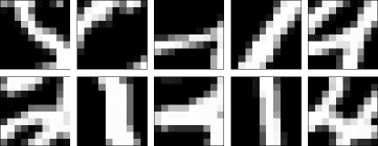
The Cmnist dataset is a low-dimensional variation on the Mnist dataset [17], containing 12,000 samples of dimension 100. The full dataset is split into training, validation and test sets of 4,000 samples each. The dataset is obtained by taking a $10\times 10$ image at the center of each Mnist sample and using the values in [0,1] as probabilities. The first 10 samples of the Cmnist dataset are shown in Figure 2.

Figure 2: First 10 samples of the Cmnist dataset.

We propose two baselines to which to compare the log-likelihood values of models trained on the Cmnist dataset:

1. The uniform coding scheme: a model which gives equal probability to all possible binary $10\times 10$ images. The log-likelihood of each sample is then $-100$ bits, or $-69.31$ nats.

2. The independent Bernoulli model in which each pixel is given an independent Bernoulli probability. The model is trained on the training set. The log-likelihood of the validation set is $-67.38$ nats per sample.

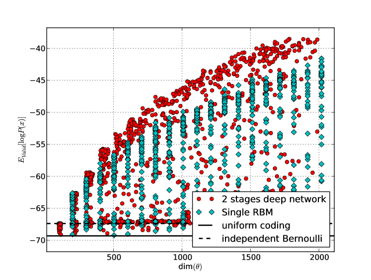
The comparison of the log-likelihood of stacked RBMs with that of single RBMs is presented in Figure 3 and confirms that the Cmnist dataset is deep.

Figure 3: Checking that Cmnist is deep: log-likelihood of the validation dataset $\mathcal{V}$ under RBMs and SRBM deep detworks selected by hyper-parameter random search, as a function of the number of parameters $\dim(\theta)$.

Tea dataset

The Tea dataset is based on the idea of learning an invariance for the amount of liquid in several containers: a teapot and 5 teacups. It contains 243 distinct samples which are then distributed into a training, validation and test set of 81 samples each. The dataset consists of $10\times 10$ images in which the left part of the image represents a (stylized) teapot of size $10\times 5$. The right part of the image represents 5 teacups of size $2\times 5$. The liquid is represented by ones and always lies at the bottom of each container. The total amount of liquid is always equal to the capacity of the teapot, i.e., there are always 50 ones and 50 zeros in any given sample. The first 10 samples of the Tea dataset are shown in Figure 4.

Figure 4: First 10 samples of the Tea dataset.

In order to better interpret the log-likelihood of models trained on the Tea dataset, we propose 3 baselines:

1. The uniform coding scheme: the baseline is the same as for the Cmnist dataset: $-69.31$ nats.

2. The independent Bernoulli model, adjusted on the training set. The log-likelihood of the validation set is $-49.27$ nats per sample.

3. The perfect model in which all $243$ samples of the full dataset (consituted by concatenation of the training, validation and test sets) are given the probability $\frac{1}{243}$. The expected log-likelihood of a sample from the validation dataset is then $\log(\frac{1}{243})=-5.49$ nats.

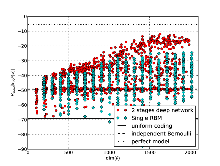
The comparison of the log-likelihood of stacked RBMs and single RBMs is presented in Figure 5 and confirms that the Tea dataset is deep.

Figure 5: Checking that Tea is deep: log-likelihood of the validation dataset $\mathcal{V}$ under RBMs and SRBM deep networks selected by hyper-parameter random search, as a function of the number of parameters $\dim(\theta)$.

3.2 Deep Generative Auto-Encoder Training

A first application of our approach is the training of a deep generative model using auto-associators. To this end, we propose to train lower layers using auto-associators and to use an RBM for the generative top layer model.

We will compare three kinds of deep architectures: standard auto-encoders with an RBM on top (vanilla AEs), the new auto-encoders with rich inference (AERIes) suggested by our framework, also with an RBM on top, and, for comparison, stacked restricted Boltzmann machines (SRBMs). All the models used in this study use the same final generative model class for $P(\mathbf{x}|\mathbf{h})$ so that the comparison focuses on the training procedure, on equal ground. SRBMs are considered the state of the art [12, 1]—although performance can be increased using richer models [3], our focus here is not on the model but on the layer-wise training procedure for a given model class.

In ideal circumstances, we would have compared the log-likelihood obtained for each training algorithm with the optimum of a deep learning procedure such as the full gradient ascent procedure (Section 2). Instead, since this ideal deep learning procedure is intractable, SRBMs serve as a reference.

The new AERIes are auto-encoders modified after the following remark: the complexity of the inference model used for $q(\mathbf{h}|\mathbf{x})$ can be increased safely without risking overfit and loss of generalization power, because $q$ is not part of the final generative model, and is used only as a tool for optimization of the generative model parameters. This would suggest that the complexity of $q$ could be greatly increased with only positive consequences on the performance of the model.

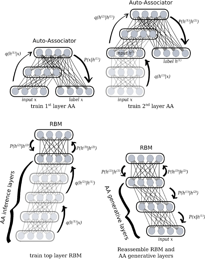
AERIes exploit this possibility by having, in each layer, a modified auto-associator with two hidden layers instead of one: $\mathbf{x}\to\mathbf{h}^{\prime}\to\mathbf{h}\to\mathbf{x}$. The generative part $P_{\theta_{I}}(\mathbf{x}|\mathbf{h})$ will be equivalent to that of a regular auto-associator, but the inference part $q(\mathbf{h}|\mathbf{x})$ will have greater representational power because it includes the hidden layer $\mathbf{h}^{\prime}$ (see Figure 7).

We will also use the more usual auto-encoders composed of auto-associators with one hidden layer and tied weights, commonly encountered in the literature (vanilla AE).

For all models, the deep architecture will be of depth $2$. The stacked RBMs will be made of two ordinary RBMs. For AERIes and vanilla AEs, the lower part is made of a single auto-associator (modified for AERies), and the generative top part is an RBM. (Thus they have one layer less than depicted for the sake of generality in Figures 6 and 7.) For AERIes and vanilla AEs the lower part of the model is trained using the usual backpropagation algorithm with cross-entropy loss, which performs gradient ascent for the probability of (25). The top RBM is then trained to maximize (12).

The competitiveness of each model will be evaluated through a comparison in log-likelihood over a validation set distinct from the training set. Comparisons are made for a given identical number of parameters of the generative model. Each model will be given equal chance to find a good optimum in terms of the number of evaluations in a hyper-parameter selection procedure by random search.

When implementing the training procedure proposed in Section 2, several approximations are needed. An important one, compared to Theorem 1, is that the distribution $q(\mathbf{h}|\mathbf{x})$ will not really be trained over all possible conditional distributions for $\mathbf{h}$ knowing $\mathbf{x}$. Next, training of the upper layers will of course fail to reproduce the BLM perfectly. Moreover, auto-associators use an $\mathbf{x}=\tilde{\mathbf{x}}$ approximation, cf. (25). We will study the effect of these approximations.

Let us now provide more details for each model.

Stacked RBMs.

For our comparisons, 1000 stacked RBMs were trained using the procedure from [12]. We used random search on the hyper-parameters, which are: the sizes of the hidden layers, the CD learning rate, and the number of CD epochs.

Vanilla auto-encoders.

The general training algorithm for vanilla auto-encoders is depicted in Figure 6. First an auto-associator is trained to maximize the adaptation of the BLM upper bound for auto-associators presented in (25). The maximization procedure itself is done with the backpropagation algorithm and cross-entropy loss. The inference weights are tied to the generative weights so that $\mathbf{W}_{\mathrm{gen}}=\mathbf{W}_{\mathrm{inf}}^{\top}$ as is often the case in practice. An ordinary RBM is used as a generative model on the top layer.

Figure 6: Deep generative auto-encoder training scheme.

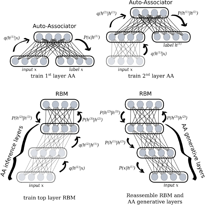
1000 deep generative auto-encoders were trained using random search on the hyper-parameters. Because deep generative auto-encoders use an RBM as the top layer, they use the same hyper-parameters as stacked RBMs, but also backpropagation (BP) learning rate, BP epochs, and ANN init $\sigma$ (i.e. the standard deviation of the gaussian used during initialization).

Auto-Encoders with Rich Inference (AERIes).

The model and training scheme for AERIes are represented in Figure 7. Just as for vanilla auto-encoders, we use the backpropagation algorithm and cross-entropy loss to maximize the auto-encoder version (25) of the BLM upper bound on the training set. No weights are tied, of course, as this does not make sense for an auto-associator with different models for $P(\mathbf{x}|\mathbf{h})$ and $q(\mathbf{h}|\mathbf{x})$. The top RBM is trained afterwards. Hyper-parameters are the same as above, with in addition the size of the new hidden layer $\mathbf{h}^{\prime}$.

Figure 7: Deep generative modified auto-encoder (AERI) training scheme.

Results

The results of the above comparisons on the Tea and Cmnist validation datasets are given in Figures 8 and 9. For better readability, the Pareto front for each model is given in Figures 10 and 11.

Figure 8: Comparison of the average validation log-likelihood for SRBMs, vanilla AE, and AERIes on the Tea dataset.

Figure 9: Comparison of the average validation log-likelihood for SRBMs, vanilla AE, and AERIes on the Cmnist dataset.

Figure 10: Pareto fronts for the average validation log-likelihood and number of parameters for SRBMs, deep generative auto-encoders, and modified deep generative auto-encoders on the Tea dataset.

Figure 11: Pareto fronts for the average validation log-likelihood and number of parameters for SRBMs, deep generative auto-encoders, and modified deep generative auto-encoders on the Cmnist dataset.

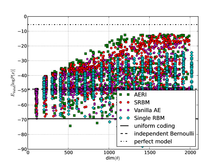
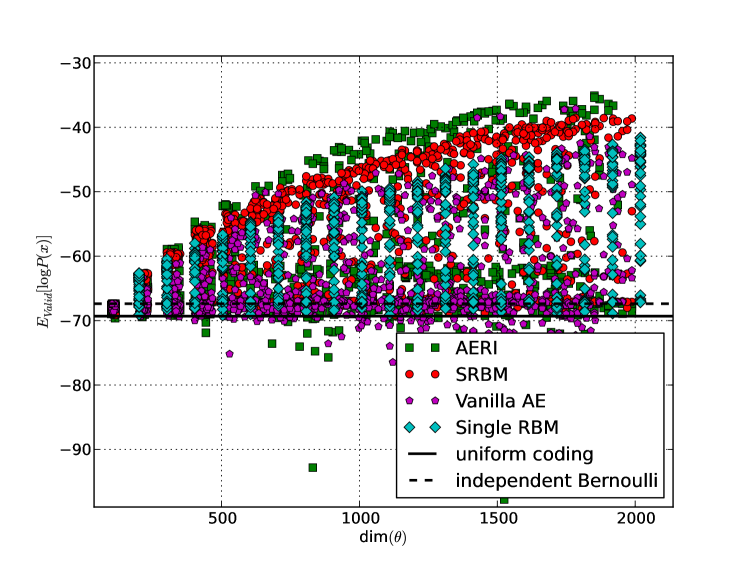
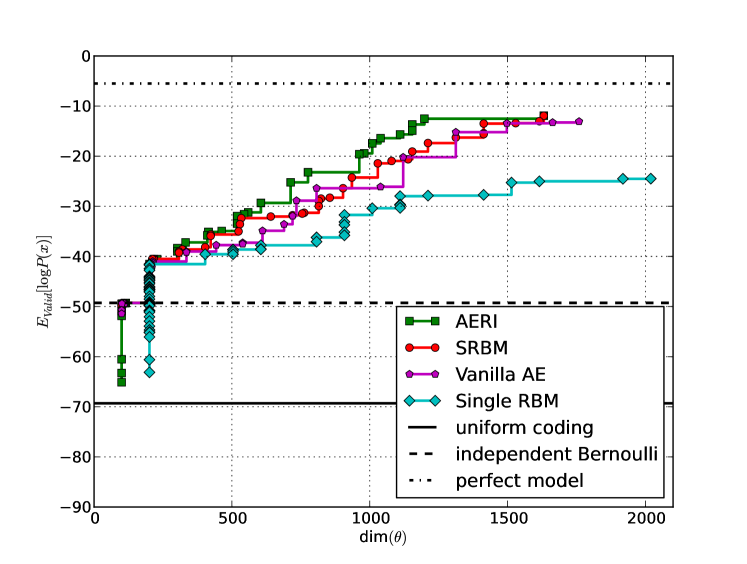
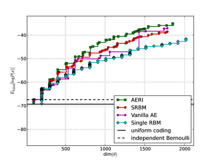
As expected, all models perform better than the baseline independent Bernoulli model but have a lower likelihood than the perfect model. Also, SRBMs, vanilla AEs and AERIes perform better than a single RBM, which can be seen as further evidence that the Tea and Cmnist are deep datasets.

Among deep models, vanilla auto-encoders achieve the lowest performance, but outperform single RBMs significantly, which validates them not only as generative models but also as deep generative models. Compared to SRBMs, vanilla auto-encoders achieve almost identical performance but the algorithm clearly suffers from local optima: most instances perform poorly and only a handful achieve performance comparable to that of SRBMs or AERIes.

As for the auto-encoders with rich inference (AERIes), they are able to outperform not only single RBMs and vanilla auto-encoders, but also stacked RBMs, and do so consistently. This validates not only the general deep learning procedure of Section 2, but arguably also the understanding of auto-encoders in this framework.

The results confirm that a more universal model for $q$ can significantly improve the performance of a model, as is clear from comparing the vanilla and rich-inference auto-encoders. Let us insist that the rich-inference auto-encoders and vanilla auto-encoders optimize over exactly the same set of generative models with the same structure, and thus are facing exactly the same optimization problem (4). Clearly the modified training procedure yields improved values of the generative parameter $\theta$.

3.3 Layer-Wise Evaluation of Deep Belief Networks

As seen in section 2, the BLM upper bound $U_{\mathcal{D}}(\theta_{I})$ is the least upper bound of the log-likelihood of deep generative models using some given $\theta_{I}$ in the lower part of the model. This raises the question of whether it is a good indicator of the final performance of $\theta_{I}$.

In this setting, there are a few approximations w.r.t. (10) and (12) that need to be discussed. Another point is the intractability of the BLM upper bound for models with many hidden variables, which leads us to propose and test an estimator in Section 3.3.4, though the experiments considered here were small enough not to need this unless otherwise specified.

We now look, in turn, at how the BLM upper bound can be applied to log-likelihood estimation, and to hyper-parameter selection—which can be considered part of the training procedure. We first discuss various possible effects, before measuring them empirically.

3.3.1 Approximations in the BLM upper bound

Consider the maximization of (14). In practice, we do not perform a specific maximization over $q$ to obtain the BLM as in (14), but rely on the training procedure of $\theta_{I}$ to maximize it. Thus the $q$ resulting from a training procedure is generally not the globally optimal $\hat{q}$ from Theorem 1. In the experiments we of course use the BLM upper bound with the value of $q$ resulting from the actual training.

Definition 8.

For $\theta_{I}$ and $q$ resulting from the training of a deep generative model, let

$$\hat{\mathcal{U}}_{\mathcal{D},q}(\theta_{I})\mathrel{\mathop{:}}=\mathbb{E}_{\mathbf{x}\sim P_{\mathcal{D}}}\left[\log\sum_{\mathbf{h}}P_{\theta_{I}}(\mathbf{x}|\mathbf{h})q_{\mathcal{D}}(\mathbf{h})\right]$$ (34)

be the empirical BLM upper bound.

This definition makes no assumption about how $\theta_{I}$ and ${q}$ in the first layer have been trained, and can be applied to any layer-wise training procedure, such as SRBMs.

Ideally, this quantity should give us an idea of the final performance of the deep architecture when we use $\theta_{I}$ on the bottom layer. But there are several discrepancies between these BLM estimates and final performance.

A first question is the validity of the approximation (34). The BLM upper bound $\mathcal{U}_{\mathcal{D}}(\theta_{I})$ is obtained by maximization over all possible $q$ which is of course untractable. The learned inference distribution ${q}$ used in practice is only an approximation for two reasons: first, because the model for $q$ may not cover all possible conditional distributions $q(\mathbf{h}|\mathbf{x})$, and, second, because the training of $q$ can be imperfect. In effect $\hat{\mathcal{U}}_{\mathcal{D},{q}}(\theta_{I})$ is only a lower bound of the BLM upper bound : $\hat{\mathcal{U}}_{\mathcal{D},{q}}(\theta_{I})\leqslant\mathcal{U}_{\mathcal{D}}(\theta_{I})$.

Second, we can question the relationship between the (un-approximated) BLM upper bound (14) and the final log-likelihood of the model. The BLM bound is optimistic, and tight only when the upper part of the model manages to reproduce the BLM perfectly. We should check how tight it is in practical applications when the upper layer model for $P(\mathbf{h})$ is imperfect.

In addition, as for any estimate from a training set, final performance on validation and test sets might be different. Performance of a model on the validation set is generally lower than on the training set. But on the other hand, in our situation there is a specific regularizing effect of imperfect training of the top layers. Indeed the BLM refers to a universal optimization over all possible distributions on $\mathbf{h}$ and might therefore overfit more, hugging the training set too closely. Thus if we did manage to reproduce the BLM perfectly on the training set, it could well decrease performance on the validation set. On the other hand, training the top layers to approximate the BLM within a model class $P_{\theta_{J}}$ introduces further regularization and could well yield higher final performance on the validation set than if the exact BLM distribution had been used.

This latter regularization effect is relevant if we are to use the BLM upper bound for hyper-parameter selection, a scenario in which regularization is expected to play an important role.

We can therefore expect:

1. That the ideal BLM upper bound, being by definition optimistic, can be higher that the final likelihood when the model obtained for $P(\mathbf{h})$ is not perfect.

2. That the empirical bound obtained by using a given conditional distribution $q$ will be lower than the ideal BLM upper bound either when $q$ belongs to a restricted class, or when $q$ is poorly trained.

3. That the ideal BLM upper bound on the training set may be either higher or lower than actual performance on a validation set, because of the regularization effect of imperfect top layer training.

All in all, the relationship between the empirical BLM upper bound used in training, and the final log-likelihood on real data, results from several effects going in both directions. This might affect whether the empirical BLM upper bound can really be used to predict the future performance of a given bottom layer setting.

3.3.2 A method for single-layer evaluation and layer-wise hyper-parameter selection

In the context of deep architectures, hyper-parameter selection is a difficult problem. It can involve as much as 50 hyper-parameters, some of them only relevant conditionally to others [5, 6]. To make matters worse, evaluating the generative performance of such models is often intractable. The evaluation is usually done w.r.t. classification performance as in [14, 5, 6], sometimes complemented by a visual comparison of samples from the model [12, 21]. In some rare instances, a variational approximation of the log-likelihood is considered [22, 21].

These methods only consider evaluating the models after all layers have been fully trained. However, since the training of deep architectures is done in a layer-wise fashion, with some criterion greedily maximized at each step, it would seem reasonable to perform a layer-wise evaluation. This would have the advantage of reducing the size of the hyper-parameter search space from exponential to linear in the number of layers.

We propose to first evaluate the performance of the lower layer, after it has been trained, according to the BLM upper bound (34) (or an approximation thereof) on the validation dataset $\mathcal{D}_{\mathrm{valid}}$. The measure of performance obtained can then be used as part of a larger hyper-parameter selection algorithm such as [6, 5]. This results in further optimization of (10) over the hyper-parameter space and is therefore justified by Theorem 1.

Evaluating the top layer is less problematic: by definition, the top layer is always a “shallow” model for which the true likelihood becomes more easily tractable. For instance, although RBMs are well known to have an intractable partition function which prevents their evaluation, several methods are able to compute close approximations to the true likelihood (such as Annealed Importance Sampling [19, 22]). The dataset to be evaluated with this procedure will have to be a sample of $\sum_{\mathbf{x}}q(\mathbf{h}|\mathbf{x})P_{\mathcal{D}}(\mathbf{x})$.

In summary, the evaluation of a two-layer generative model can be done in a layer-wise manner:

1. Perform hyper-parameter selection on the lower layer using $\hat{\mathcal{U}}_{\theta_{I}}(\mathcal{D})$ as a performance measure (preferably on a validation rather than training dataset, see below), and keep only the best possible lower layers according to this criterion.

2. Perform hyper-parameter selection on the upper layer by evaluating the true likelihood of validation data samples transformed by the inference distribution, under the model of the top layer.

Hyper-parameter selection was not used in our experiments, where we simply used hyper-parameter random search. (This has allowed, in particular, to check the robustness of the models, as AERIes have been found to perform better than vanilla AEs on many more instances over hyper-parameter space.)

As mentioned earlier, in the context of representation learning the top layer is irrelevant because the objective is not to train a generative model but to get a better representation of the data. With the assumption that good latent variables make good representations, this suggests that the BLM upper bound can be used directly to select the best possible lower layers.

3.3.3 Testing the BLM and its approximations

We now present a series of tests to check whether the selection of lower layers with higher values of the BLM actually results in higher log-likelihood for the final deep generative models, and to assess the quantitative importance of each of the BLM approximations discussed earlier.

For each training algorithm (SRBMs, RBMs, AEs, AERIes), the comparison is done using 1000 models trained with hyper-parameters selected through random search as before. The empirical BLM upper bound is computed using (34) above.

Training BLM upper bound vs training log-likelihood.

We first compare the value of the empirical BLM upper bound $\hat{\mathcal{U}}_{\theta_{I}}(\mathcal{D}_{\mathrm{train}})$ over the training set, with the actual log-likelihood of the trained model on the training set. This is an evaluation of how optimistic the BLM is for a given dataset, by checking how closely the training of the upper layers manages to match the target BLM distribution on $\mathbf{h}$. This is also the occasion to check the effect of using the ${q}(\mathbf{h}|\mathbf{x})$ resulting from actual learning, instead of the best $q$ in all possible conditional distributions.

In addition, as discussed below, this comparison can be used as a criterion to determine whether more layers should be added to the model.

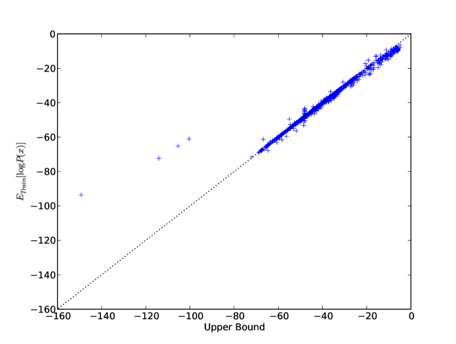
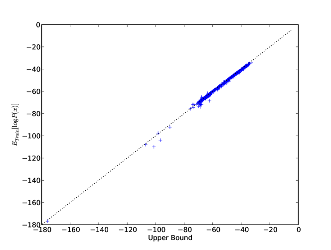
The results are given in Figures 12 and 13 for SRBMs, and 14 and 15 for AERIes. We see that the empirical BLM upper bound (34) is a good predictor of the future log-likelihood of the full model on the training set. This shows that the approximations w.r.t. the optimality of the top layer and the universality of $q$ can be dealt with in practice.

For AERIes, a few models with low performance have a poor estimation of the BLM upper bound (estimated to be lower than the actual likelihood), presumably because of a bad approximation in the learning of $q$. This will not affect model selection procedures as it only concerns models with very low performance, which are to be discarded.

Figure 12: Comparison of the BLM upper bound on the first layer and the final log-likelihood on the Tea training dataset, for 1000 2-layer SRBMs

Figure 13: Comparison of the BLM upper bound on the first layer and the final log-likelihood on the Cmnist training dataset, for 1000 2-layer SRBMs

Figure 14: Comparison of the BLM upper bound on the first layer and the final log-likelihood on the Tea training dataset, for 1000 2-layer AERIes

Figure 15: Comparison of the BLM upper bound on the first layer and the final log-likelihood on the Cmnist training dataset, for 1000 2-layer AERIes

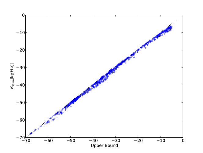
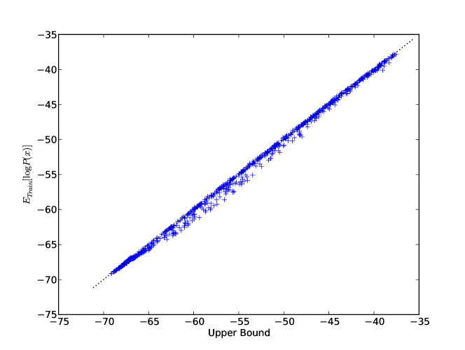
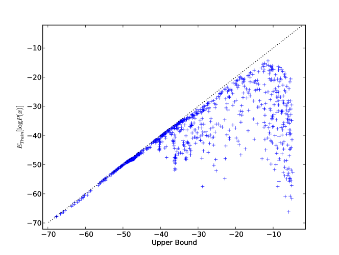
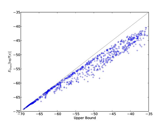
If the top part of the model were not powerful enough (e.g., if the network is not deep enough), the BLM upper bound would be too optimistic and thus significantly higher than the final log-likelihood of the model. To further test this intuition we now compare the BLM upper bound of the bottom layer with the log-likelihood obtained by a shallow architecture with only one layer; the difference would give an indication of how much could be gained by adding top layers. Figures 16 and 17 compare the expected log-likelihood of the training set under the 1000 RBMs previously trained with the BLM upper bound for a generative model using this RBM as first layer. The results contrast with the previous ones and confirm that final performance is below the BLM upper bound when the model does not have enough layers.

Figure 16: BLM on a too shallow model: comparison of the BLM upper bound and the AIS log-likelihood of an RBM on the Tea training dataset

Figure 17: BLM on a too shallow model: Comparison of the BLM upper bound and the AIS log-likelihood of an RBM on the Cmnist training dataset

The alignment in Figures 12 and 13 can therefore be seen as a confirmation that the Tea and Cmnist datasets would not benefit from a third layer.

Thus, the BLM upper bound could be used as a test for the opportunity of adding layers to a model.

Training BLM upper bound vs validation log-likelihood.

We now compare the training BLM upper bound with the log-likelihood on a validation set distinct from the training set: this tests whether the BLM obtained during training is a good indication of the final performance of a bottom layer parameter.

Figure 18: Training BLM upper bound vs validation log-likelihood on the Tea training dataset

Figure 19: Training BLM upper bound vs validation log-likelihood on the Cmnist training dataset

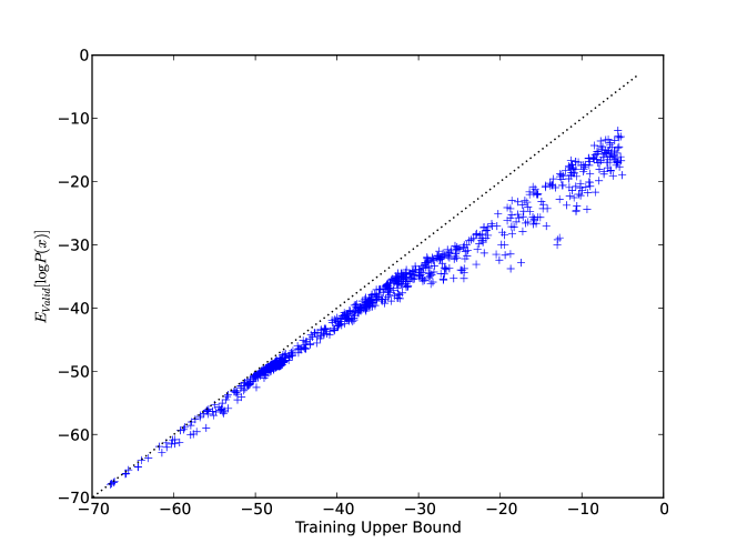
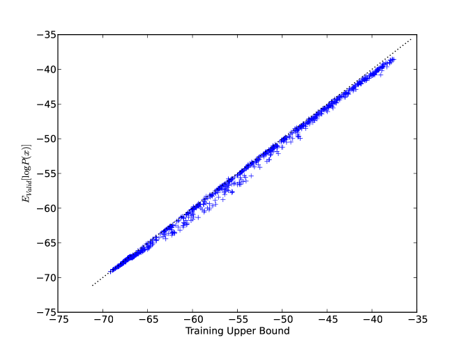
As discussed earlier, because the BLM makes an assumption where there is no regularization, using the training BLM upper bound to predict performance on a validation set could be too optimistic: therefore we expect the validation log-likelihood to be somewhat lower than the training BLM upper bound. (Although, paradoxically, this can be somewhat counterbalanced by imperfect training of the upper layers, as mentioned above.)

The results are reported in Figures 18 and 19 and confirm that the training BLM is an upper bound of the validation log-likelihood. As for regularization, we can see that on the Cmnist dataset where there are $4000$ samples, generalization is not very difficult: the optimal $P(\mathbf{h})$ for the training set used by the BLM is in fact almost optimal for the validation set too. On the Tea dataset, the picture is somewhat different: there is a gap between the training upper-bound and the validation log-likelihood. This can be attributed to the increased importance of regularization on this dataset in which the training set contains only $81$ samples.

Although the training BLM upper bound can therefore not be considered a good predictor of the validation log-likelihood, it is still a monotonous function of the validation log-likelihood: as such it can still be used for comparing parameter settings and for hyper-parameter selection.

Feeding the validation dataset to the BLM.

Predictivity of the BLM (e.g., for hyper-parameter selection) can be improved by feeding the validation rather than training set to the inference distribution and the BLM.

In the cases above we examined the predictivity of the BLM obtained during training, on final performance on a validation dataset. We have seen that the training BLM is an imperfect predictor of this performance, notably because of lack of regularization in the BLM optimistic assumption, and because we use an inference distribution $q$ maximized over the training set.

Some of these effects can easily be predicted by feeding the validation set to the BLM and the inference part of the model during hyper-parameter selection, as follows.

We call validation BLM upper bound the BLM upper bound obtained by using the validation dataset instead of $\mathcal{D}$ in (34). Note that the values $q$ and $\theta_{I}$ are still those obtained from training on the training dataset. This parallels the validation step for auto-encoders, in which, of course, reconstruction performance on a validation dataset is done by feeding this same dataset to the network.

We now compare the validation BLM upper bound to the log-likelihood of the validation dataset, to see if it qualifies as a reasonable proxy.

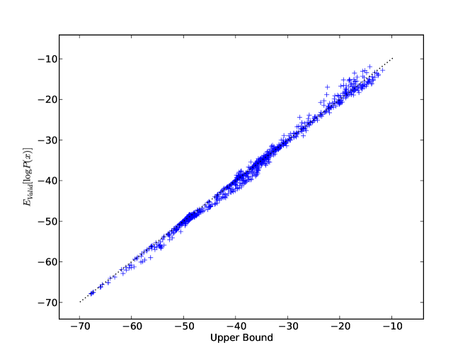
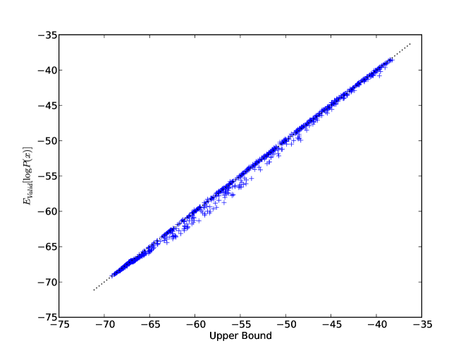
The results are reported in Figures 20 and 21. As predicted, the validation BLM upper bound is a better estimator of the validation log-likelihood (compare Figures 18 and 19).

We can see that several models have a validation log-likelihood higher than the validation BLM upper bound, which might seem paradoxical. This is simply because the validation BLM upper bound still uses the parameters trained on the training set and thus is not formally an upper bound.

The better overall approximation of the validation log-likelihood seems to indicate that performing hyper-parameter selection with the validation BLM upper bound can better account for generalization and regularization.

Figure 20: Validation upper bound vs log-likelihood on the Tea validation dataset

Figure 21: Validation upper bound vs log-likelihood on the Cmnist validation dataset

3.3.4 Approximating the BLM for larger models

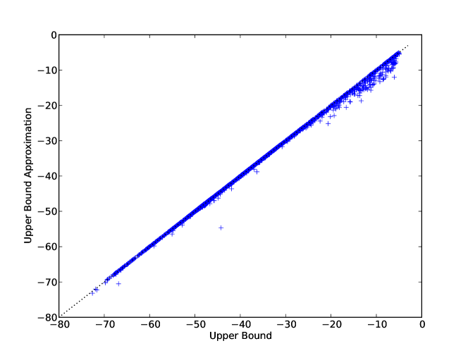
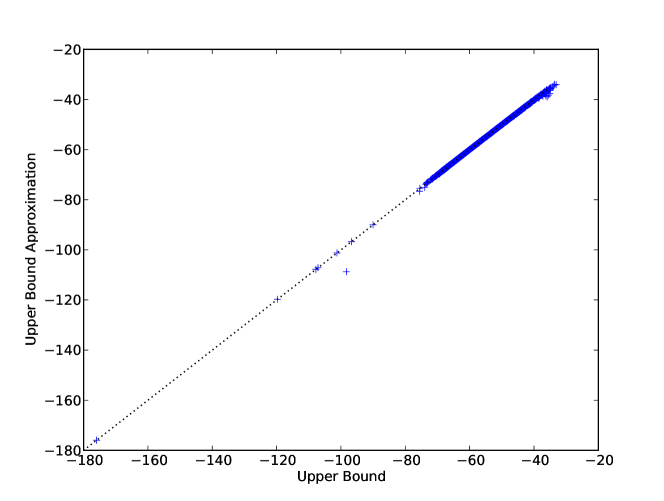
The experimental setting considered here was small enough to allow for an exact computation of the various BLM bounds by summing over all possible states of the hidden variable $\mathbf{h}$. However the exact computation of the BLM upper bound using $\hat{\mathcal{U}}_{\mathcal{D},{q}}(\theta_{I})$ as in (34) is not always possible because the number of terms in this sum is exponential in the dimension of the hidden layer $\mathbf{h}$.

In this situation we can use a sampling approach. For each data sample $\tilde{\mathbf{x}}$, we can take $K$ samples from each mode of the BLM distribution $q_{\mathcal{D}}$ (one mode for each data sample $\mathbf{\tilde{x}}$) to obtain an approximation of the upper bound in $\mathcal{O}(K\times N^{2})$ where $N$ is the size of the validation set. (Since the practitioner can choose the size of the validation set which need not necessarily be as large as the training or test sets, we do not consider the $N^{2}$ factor a major hurdle.)

Definition 9.

For $\theta_{I}$ and ${q}$ resulting from the training of a deep generative model, let

$$\hat{\hat{\mathcal{U}}}_{\mathcal{D},q}(\theta_{I})\mathrel{\mathop{:}}=\mathbb{E}_{\mathbf{x}\sim P_{\mathcal{D}}}\left[\log\sum_{\mathbf{\tilde{x}}}\sum_{k=1}^{K}P_{\theta_{I}}(\mathbf{x}|\mathbf{h})q(\mathbf{h}|\mathbf{\tilde{x}})P_{\mathcal{D}}(\mathbf{\tilde{x}})\right]$$ (35)

where for each $\tilde{\mathbf{x}}$ and $k$, $\mathbf{h}$ is sampled from $q(\mathbf{h}|\tilde{\mathbf{x}})$.

To assess the accuracy of this approximation, we take $K=1$ and compare the values of $\hat{\hat{\mathcal{U}}}_{\mathcal{D},{q}}(\theta_{I})$ and of $\hat{\mathcal{U}}_{\mathcal{D},{q}}(\theta_{I})$, on the Cmnist and Tea training datasets. The results are reported in Figures 22 and 23 for all three models (vanilla AEs, AERIes, and SRBMs) superimposed, showing good agreement.

Figure 22: Approximation of the training BLM upper bound on the Tea training dataset

Figure 23: Approximation of the training BLM upper bound on the the Cmnist training dataset

Conclusions

The new layer-wise approach we propose to train deep generative models is based on an optimistic criterion, the BLM upper bound, in which we suppose that learning will be successful for upper layers of the model. Provided this optimism is justified a posteriori and a good enough model is found for the upper layers, the resulting deep generative model is provably close to optimal. When optimism is not justified, we provide an explicit bound on the loss of performance.

This provides a new justification for auto-encoder training and fine-tuning, as the training of the lower part of a deep generative model, optimized using a lower bound on the BLM.

This new framework for training deep generative models highlights the importance of using richer models when performing inference, contrary to current practice. This is consistent with the intuition that it is much harder to guess the underlying structure by looking at the data, than to derive the data from the hidden structure once it is known.

This possibility is tested empirically with auto-encoders with rich inference (AERIes) which are completed with a top-RBM to create deep generative models: these are then able to outperform current state of the art (stacked RBMs) on two different deep datasets.

The BLM upper bound is also found to be a good layer-wise proxy to evaluate the log-likelihood of future models for a given lower layer setting, and as such is a relevant means of hyper-parameter selection.

This opens new avenues of research, for instance in the design of algorithms to learn features in the lower part of the model, or in the possibility to consider feature extraction as a partial deep generative model in which the upper part of the model is temporarily left unspecified.

References

- [1] Y. Bengio, P. Lamblin, V. Popovici, and H. Larochelle. Greedy layer-wise training of deep networks. In B. Schölkopf, J. Platt, and T. Hoffman, editors, Advances in Neural Information Processing Systems 19, pages 153–160. MIT Press, Cambridge, MA, 2007.
- [2] Y. Bengio and Y. LeCun. Scaling learning algorithms towards ai. In Large-Scale Kernel Machines. MIT Press, 2007.
- [3] Yoshua Bengio, Aaron C. Courville, and Pascal Vincent. Unsupervised feature learning and deep learning: A review and new perspectives. CoRR, abs/1206.5538, 2012.
- [4] Yoshua Bengio and Olivier Delalleau. Justifying and generalizing contrastive divergence. Neural Computation, 21(6):1601–1621, 2009.
- [5] James Bergstra, Rémy Bardenet, Yoshua Bengio, and Balázs Kégl. Algorithms for hyper-parameter optimization. In Advances in Neural Information Processing Systems 23, 2011.
- [6] James Bergstra and Yoshua Bengio. Random search for hyper-parameter optimization. Journal of Machine Learning Research, 13:281–305, 2012.
- [7] H. Bourlard and Y. Kamp. Auto-association by multilayer perceptrons and singular value decomposition. Biological Cybernetics, 59:291–294, 1988.
- [8] Wray L. Buntine and Andreas S. Weigend. Bayesian back-propagation. Complex Systems, 5:603–643, 1991.
- [9] Thomas M. Cover and Joy A. Thomas. Elements of information theory. Wiley-Interscience [John Wiley & Sons], Hoboken, NJ, second edition, 2006.
- [10] A. P. Dempster, N. M. Laird, and D. B. Rubin. Maximum likelihood from incomplete data via the EM algorithm. Journal of the Royal Statistical Society. Series B (Methodological), 39:1–38, 1977.
- [11] G.E. Hinton. Training products of experts by minimizing contrastive divergence. Neural Computation, 14:1771–1800, 2002.
- [12] G.E. Hinton, S. Osindero, and Yee-Whye Teh. A fast learning algorithm for deep belief nets. Neural Conputation, 18:1527–1554, 2006.
- [13] G.E. Hinton and R. Salakhutdinov. Reducing the dimensionality of data with neural networks. Science, 313(5786):504–507, July 2006.
- [14] H. Larochelle, Y. Bengio, J. Louradour, and P. Lamblin. Exploring strategies for training deep neural networks. The Journal of Machine Learning Research, 10:1–40, 2009.
- [15] H. Larochelle, D. Erhan, A. Courville, J. Bergstra, and Y. Bengio. An empirical evaluation of deep architectures on problems with many factors of variation. In ICML ’07: Proceedings of the 24th international conference on Machine learning, pages 473–480, New York, NY, USA, 2007. ACM.
- [16] Nicolas Le Roux and Yoshua Bengio. Representational power of restricted Boltzmann machines and deep belief networks. Neural Computation, 20:1631–1649, June 2008.
- [17] Y. LeCun, L. Bottou, Y. Bengio, and P. Haffner. Gradient-based learning applied to document recognition. Proceedings of the IEEE, 86(11):2278–2324, November 1998.
- [18] R. M. Neal. Learning stochastic feedforward networks. Technical report, Dept. of Computer Science, University of Toronto, 1990.
- [19] Radford M. Neal. Annealed importance sampling. Technical report, University of Toronto, Department of Statistics, 1998.
- [20] Salah Rifai, Yoshua Bengio, Yann Dauphin, and Pascal Vincent. A generative process for sampling contractive auto-encoders. In International Conference on Machine Learning, ICML’12, 06 2012.
- [21] Ruslan Salakhutdinov and Geoffrey Hinton. Deep Boltzmann machines. In Proceedings of the Twelfth International Conference on Artificial Intelligence and Statistics (AISTATS), volume 5, pages 448–455, 2009.
- [22] Ruslan Salakhutdinov and Iain Murray. On the quantitative analysis of deep belief networks. In Proceedings of the 25th international conference on Machine learning, ICML ’08, pages 872–879, New York, NY, USA, 2008. ACM.
- [23] P. Smolensky. Information processing in dynamical systems: foundations of harmony theory. In D. Rumelhart and J. McClelland, editors, Parallel Distributed Processing, volume 1, chapter 6, pages 194–281. MIT Press, Cambridge, MA, USA, 1986.
- [24] Pascal Vincent, Hugo Larochelle, Yoshua Bengio, and Pierre-Antoine Manzagol. Extracting and composing robust features with denoising autoencoders. In Proceedings of the 25th international conference on Machine learning, ICML ’08, pages 1096–1103, New York, NY, USA, 2008.
- [25] C. F. Jeff Wu. On the convergence properties of the EM algorithm. The Annals of Statistics, 11:95–103, 1983.