Infinite swapping replica exchange molecular dynamics leads to
a simple simulation patch using mixture potentials

Abstract

Replica exchange molecular dynamics (REMD) becomes more efficient as the frequency of swap between the temperatures is increased. Recently in [Plattner et al. J. Chem. Phys. 135, 134111 (2011)] a method was proposed to implement infinite swapping REMD in practice. Here we introduce a natural modification of this method that involves molecular dynamics simulations over a mixture potential. This modification is both simple to implement in practice and provides a better, energy based understanding of how to choose the temperatures in REMD to optimize efficiency. It also opens the door to generalizations of REMD in which the swaps involve other parameters than the temperature.

I Introduction

Replica exchange molecular dynamics (REMD) is one of the most popular methods to accelerate the conformational sampling of large biomolecules and other complex molecular systems Hansmann (1997); Sugita and Okamoto (1999); Sugita et al. (2000); Rao and Caflisch (2003); Earl and Deem (2005). It can be viewed as a generalization to molecular dynamics (MD) simulations of the replica exchange Monte Carlo method Swendsen and Wang (1986); Geyer (1991); Geyer and Thompson (1995); Hukushima and Nemoto (1996); Marinari et al. (1998); Tesi et al. (1996). The basic idea of REMD is to evolve concurrently several copies (or replica) of the system, and periodically swap their temperatures in a thermodynamically consistent way. When a replica feels an artificially high temperature, it explores its conformation space much faster than it would at the physical temperature; when it feels the physical temperature, equilibrium averages can be extracted from its dynamics. In theory, the efficiency of REMD increases when the frequency of swaps is pushed up to infinity, but reaching this limit has proven difficult in practice Sindhikara et al. (2008); Abraham and Gready (2008). Recently in Ref. Plattner et al., 2011, Plattner et al. have proposed a way to avoid this difficulty. The idea is to first establish analytically what the limiting dynamics of REMD is at infinite swapping frequency, and then implement this dynamics directly instead of trying to increase the swapping frequency in the original REMD. Our main purpose here is to show that a natural reformulation of the technique of Ref. Plattner et al., 2011 leads to a simple method in which the various replica in infinite swapping REMD evolve by standard MD over a new potential that is a temperature-dependent mixture of the original one which couples all the replica. This new method is simple to implement, and reduces to a patch of standard MD codes in which several replica of the system are evolved in parallel using forces that are the original molecular ones multiplied by factors that involve the energies of the replicas: these energies are the only quantities that must be communicated between the replicas as they evolve. The method gives a new perspective on how to optimally choose the temperatures (including how many of them to pick), with implications for the original REMD, by analyzing simple geometrical characteristics of the mixture potential. As we show below, it also permits to design generalizations of REMD in which parameters other than the temperature are used to build the mixture potential.

II Infinite swapping REMD

For the sake of simplicity we will consider first the case of a system governed by the overdamped Langevin equation (the generalization to standard MD will be given in Sec. III below):

$$\dot{\boldsymbol{x}}=\boldsymbol{f}(\boldsymbol{x})+\sqrt{2\beta^{-1}}\,\boldsymbol{\eta},$$ (1)

where $\boldsymbol{x}\in\mathbb{R}^{3n}$ denotes the instantaneous position of the system with $n$ particles, $\boldsymbol{f}(\boldsymbol{x})=-\nabla V(\boldsymbol{x})$ is the force associated with the potential $V(\boldsymbol{x})$, $\beta=1/k_{B}T$ is the inverse temperature, $\boldsymbol{\eta}$ is a $3n$-dimensional white-noise and we set the friction coefficient to one for simplicity. The solutions of (1) sample the Boltzmann equilibrium probability density,

$$\rho_{\beta}(\boldsymbol{x})=Z_{\beta}^{-1}e^{-\beta V(\boldsymbol{x})}$$ (2)

where $Z_{\beta}=\int_{\mathbb{R}^{3n}}e^{-\beta V(\boldsymbol{x})}d\boldsymbol{x}$. Assuming we only take two temperatures (the generalization to more temperatures is considered in Sec. VI below), the idea behind REMD is to replace (1) by

$$\begin{cases}\dot{\boldsymbol{x}}_{1}=\boldsymbol{f}(\boldsymbol{x}_{1})+\sqrt{2\beta_{1}^{-1}(t)}\,\boldsymbol{\eta}_{1},\\ \dot{\boldsymbol{x}}_{2}=\boldsymbol{f}(\boldsymbol{x}_{2})+\sqrt{2\beta_{2}^{-1}(t)}\,\boldsymbol{\eta}_{2}\end{cases}$$ (3)

where $\boldsymbol{x}_{1}(t)$ and $\boldsymbol{x}_{2}(t)$ are the two replica, and $\beta_{1}(t)$ and $\beta_{2}(t)$ are the two temperatures that alternatively swap between the physical $\beta$ and the artificial $\bar{\beta}<\beta$ (so that $k_{B}\bar{T}>k_{B}T$). These swaps are attempted with frequency $\nu$, and the ones from $(\beta_{1},\beta_{2})=(\beta,\bar{\beta})$ to $(\beta_{1},\beta_{2})=(\bar{\beta},\beta)$ are accepted with probability

$$\min\left(\frac{\rho_{\bar{\beta}}(\boldsymbol{x}_{1})\rho_{\beta}(\boldsymbol{x}_{2})}{\rho_{\beta}(\boldsymbol{x}_{1})\rho_{\bar{\beta}}(\boldsymbol{x}_{2})},1\right)$$ (4)

and similarly for the ones from $(\beta_{1},\beta_{2})=(\bar{\beta},\beta)$ to $(\beta_{1},\beta_{2})=(\beta,\bar{\beta})$. (4) is the standard acceptance probability used in Metropolis Monte Carlo schemes and it guarantees that (3) samples the following equilibrium probability distribution in $(\boldsymbol{x}_{1},\beta_{1},\boldsymbol{x}_{2},\beta_{2})$:

$$\boldsymbol{\varrho}_{\beta,\bar{\beta}}(\boldsymbol{x}_{1},\beta_{1},\boldsymbol{x}_{2},\beta_{2})$$ (5)

$$=\rho_{\beta_{1}}(\boldsymbol{x}_{1})\rho_{\beta_{2}}(\boldsymbol{x}_{2})\left(\tfrac{1}{2}\delta_{\beta_{1},\beta}\delta_{\beta_{2},\bar{\beta}}+\tfrac{1}{2}\delta_{\beta_{1},\bar{\beta}}\delta_{\beta_{2},\beta}\right)$$

where $\delta_{\beta_{1},\beta}$ denotes the Kronecker delta function, $\delta_{\beta_{1},\beta}=1$ if $\beta_{1}=\beta$ and $\delta_{\beta_{1},\beta}=0$ otherwise. Summing over $(\beta_{1},\beta_{2})$ then gives the equilibrium density for the replica positions alone, which is a symmetrized version of the Boltzmann densities at the two temperatures $\beta$ and $\bar{\beta}$:

$$\varrho_{\beta,\bar{\beta}}(\boldsymbol{x}_{1},\boldsymbol{x}_{2})=\tfrac{1}{2}\rho_{\beta}(\boldsymbol{x}_{1})\rho_{\bar{\beta}}(\boldsymbol{x}_{2})+\tfrac{1}{2}\rho_{\bar{\beta}}(\boldsymbol{x}_{1})\rho_{\beta}(\boldsymbol{x}_{2})$$ (6)

As a result the ensemble average at the physical temperature of any observable $A(\boldsymbol{x})$ can be estimated from

$$\langle A\rangle_{\beta} \equiv\int_{\mathbb{R}^{3n}}A(\boldsymbol{x})\rho_{\beta}(\boldsymbol{x})d\boldsymbol{x}$$ (7)

$$=\int\limits_{\mathbb{R}^{3n}\times\mathbb{R}^{3n}}\big{(}\omega_{\beta,\bar{\beta}}(\boldsymbol{x}_{1},\boldsymbol{x}_{2})A(\boldsymbol{x}_{1})+\omega_{\bar{\beta},\beta}(\boldsymbol{x}_{1},\boldsymbol{x}_{2})A(\boldsymbol{x}_{2})\big{)}\varrho_{\beta,\bar{\beta}}(\boldsymbol{x}_{1},\boldsymbol{x}_{2})d\boldsymbol{x}_{1}d\boldsymbol{x}_{2}$$

$$=\lim_{T\to\infty}\frac{1}{T}\int_{0}^{T}\big{(}\omega_{\beta,\bar{\beta}}(\boldsymbol{x}_{1}(t),\boldsymbol{x}_{2}(t))A(\boldsymbol{x}_{1}(t))+\omega_{\bar{\beta},\beta}(\boldsymbol{x}_{1}(t),\boldsymbol{x}_{2}(t))A(\boldsymbol{x}_{2}(t))\big{)}dt$$

where we defined the weight

$$\omega_{\beta,\bar{\beta}}(\boldsymbol{x}_{1},\boldsymbol{x}_{2}) =\frac{\rho_{\beta}(\boldsymbol{x}_{1})\rho_{\bar{\beta}}(\boldsymbol{x}_{2})}{\rho_{\beta}(\boldsymbol{x}_{1})\rho_{\bar{\beta}}(\boldsymbol{x}_{2})+\rho_{\beta}(\boldsymbol{x}_{2})\rho_{\bar{\beta}}(\boldsymbol{x}_{1})}$$ (8)

$$=\frac{e^{-\beta V(\boldsymbol{x}_{1})-\bar{\beta}V(\boldsymbol{x}_{2})}}{e^{-\beta V(\boldsymbol{x}_{1})-\bar{\beta}V(\boldsymbol{x}_{2})}+e^{-\bar{\beta}V(\boldsymbol{x}_{1})-\beta V(\boldsymbol{x}_{2})}}$$

The estimator (7) is slightly different from the one traditionally used in REMD Sugita and Okamoto (1999), but its validity can be readily checked by inserting (6) and (8) in (7), and it will prove more convenient for our purpose. To quantify the efficiency of this estimator, notice that

$$\int\limits_{\mathbb{R}^{3n}\times\mathbb{R}^{3n}}\big{(}\omega_{\beta,\bar{\beta}}A(\boldsymbol{x}_{1})+\omega_{\bar{\beta},\beta}A(\boldsymbol{x}_{2})\big{)}^{2}\varrho_{\beta,\bar{\beta}}d\boldsymbol{x}_{1}d\boldsymbol{x}_{2}$$ (9)

$$\quad\leq 2\int\limits_{\mathbb{R}^{3n}\times\mathbb{R}^{3n}}\big{(}\omega^{2}_{\beta,\bar{\beta}}A^{2}(\boldsymbol{x}_{1})+\omega^{2}_{\bar{\beta},\beta}A^{2}(\boldsymbol{x}_{2})\big{)}\varrho_{\beta,\bar{\beta}}d\boldsymbol{x}_{1}d\boldsymbol{x}_{2}$$

$$\quad\leq 2\int\limits_{\mathbb{R}^{3n}\times\mathbb{R}^{3n}}\big{(}\omega_{\beta,\bar{\beta}}A^{2}(\boldsymbol{x}_{1})+\omega_{\bar{\beta},\beta}A^{2}(\boldsymbol{x}_{2})\big{)}\varrho_{\beta,\bar{\beta}}d\boldsymbol{x}_{1}d\boldsymbol{x}_{2}$$

$$\quad=4\langle A^{2}\rangle_{\beta}$$

where $\omega_{\beta,\bar{\beta}}\equiv\omega_{\beta,\bar{\beta}}(\boldsymbol{x}_{1},\boldsymbol{x}_{2})$, $\omega_{\bar{\beta},\beta}\equiv\omega_{\bar{\beta},\beta}(\boldsymbol{x}_{1},\boldsymbol{x}_{2})$ and $\varrho_{\beta,\bar{\beta}}\equiv\varrho_{\beta,\bar{\beta}}(\boldsymbol{x}_{1},\boldsymbol{x}_{2})$, and we used the property that $0\leq\omega_{\beta,\bar{\beta}}\leq 1$. Therefore, the variance of the estimator (7) is controlled by the variance of $A(\boldsymbol{x})$ under the original density $\rho_{\beta}(\boldsymbol{x})$. This means that the efficiency of this estimator is determined by how fast the coupled system (3) converges towards equilibrium. As mentioned before, the higher $\nu$, the faster this convergence is Sindhikara et al. (2008); Abraham and Gready (2008); Plattner et al. (2011); Dupuis et al. (2012), but large values of $\nu$ requires one to make many swapping attempts, which slows down the simulations. The key observation made in Ref. Plattner et al., 2011 is that the limit $\nu\to\infty$ can be taken explicitly. In this limit, the fast temperatures are adiabatically slaved to the positions of the slow replica, and these replica only feel their average effect. This leads to the following closed equation for the replica positions replacing (3):

$$\begin{cases}\dot{\boldsymbol{x}}_{1}=\boldsymbol{f}(\boldsymbol{x}_{1})+\sqrt{2(\beta^{-1}\omega_{\beta,\bar{\beta}}+\bar{\beta}^{-1}\omega_{\bar{\beta},\beta})}\,\boldsymbol{\eta}_{1},\\ \dot{\boldsymbol{x}}_{2}=\boldsymbol{f}(\boldsymbol{x}_{2})+\sqrt{2(\bar{\beta}^{-1}\omega_{\beta,\bar{\beta}}+\beta^{-1}\omega_{\bar{\beta},\beta})}\,\boldsymbol{\eta}_{2}\end{cases}$$ (10)

Thus, simulating with (10) instead of (3) is a concrete way to perform infinite swapping REMD, and several strategies to perform these simulations were discussed in Ref. Plattner et al., 2011. Here we would like to take advantage of these strategies but simplify their implementation by modifying (10). How to do so is explained next.

III Reformulation

The system (10) is quite complicated to simulate because it involves a multiplicative noise. Yet because this system satisfies detailed balance like the original REMD (3) does, it has a specific structure that can be used to simplify it. To see how, note that the Fokker-Planck equation for the joint probability density of $\boldsymbol{x}_{1}(t)$ and $\boldsymbol{x}_{2}(t)$, $\varrho(t,\boldsymbol{x}_{1},\boldsymbol{x}_{2})$, can be written as

$$\partial_{t}\varrho(t)=\text{div}\big{(}\mathbb{B}\left(\varrho(t)\,\text{grad}\,U+k_{B}T\,\text{grad}\,\varrho(t)\right)\big{)}$$ (11)

Here div and grad denote, respectively, the divergence and gradient operators with respect to $(\boldsymbol{x}_{1},\boldsymbol{x}_{2})$, and we defined the mixture potential

$$U(\boldsymbol{x}_{1},\boldsymbol{x}_{2})$$ (12)

$$=-k_{B}T\ln\left(e^{-\beta V(\boldsymbol{x}_{1})-\bar{\beta}V(\boldsymbol{x}_{2})}+e^{-\bar{\beta}V(\boldsymbol{x}_{1})-\beta V(\boldsymbol{x}_{2})}\right)$$

as well as the tensor $\mathbb{B}\equiv\mathbb{B}(\boldsymbol{x}_{1},\boldsymbol{x}_{2})$:

$$\mathbb{B}=\begin{pmatrix}\omega_{\beta,\bar{\beta}}+\beta\bar{\beta}^{-1}\omega_{\bar{\beta},\beta}&0\\ 0&\omega_{\bar{\beta},\beta}+\beta\bar{\beta}^{-1}\omega_{\beta,\bar{\beta}}\end{pmatrix}.$$ (13)

It is easy to check that the stationary solution of (11) is $\varrho(t,\boldsymbol{x}_{1},\boldsymbol{x}_{2})=\varrho_{\beta,\bar{\beta}}(\boldsymbol{x}_{1},\boldsymbol{x}_{2})$, confirming that the limiting equation (10) samples (6) like (3) does and therefore can be used in the estimator (7). The multiplicative nature of the noise in (10) is a direct consequence of the fact that the tensor $\mathbb{B}$ in (11) depends on $\boldsymbol{x}_{1}$ and $\boldsymbol{x}_{2}$. Therefore, a natural simplification is to replace $\mathbb{B}$ by a constant tensor, which, for convenience, we will simply take to be the identity. This substitution does not affect the stationary solution of (11), but it changes the system of overdamped Langevin equations this Fokker-Planck equation is associated with. After some straightforward algebra, it is easy to see that this new system is

$$\begin{cases}\dot{\boldsymbol{x}}_{1}=(\omega_{\beta,\bar{\beta}}+\beta^{-1}\bar{\beta}\omega_{\bar{\beta},\beta})\boldsymbol{f}(\boldsymbol{x}_{1})+\sqrt{2\beta^{-1}}\,\boldsymbol{\eta}_{1},\\ \dot{\boldsymbol{x}}_{2}=(\omega_{\bar{\beta},\beta}+\beta^{-1}\bar{\beta}\omega_{\beta,\bar{\beta}})\boldsymbol{f}(\boldsymbol{x}_{2})+\sqrt{2\beta^{-1}}\,\boldsymbol{\eta}_{2}.\end{cases}$$ (14)

This system of equations samples (6) like (10) does, and its solution can be used in the estimator (7). But in contrast with (10), the noise in (14) is simply additive like in the original equation (1). The only things that have changed in (14) are the forces, which are the gradients with respect to $\boldsymbol{x}_{1}$ and $\boldsymbol{x}_{2}$ of the mixture potential (12). As can be seen from (14), these gradients involve the original forces, $\boldsymbol{f}(\boldsymbol{x}_{1})$ and $\boldsymbol{f}(\boldsymbol{x}_{2})$, multiplied by scalar factors containing the weight (8). This means that the only quantities that must be communicated between the replicas are the potential energies $V(\boldsymbol{x}_{1})$ and $V(\boldsymbol{x}_{2})$ that enter this weight.

In practice, rather than (1) one is typically interested in systems governed by the Langevin equation

$$\begin{cases}\dot{\boldsymbol{x}}=m^{-1}\boldsymbol{p},\\ \dot{\boldsymbol{p}}=\boldsymbol{f}(\boldsymbol{x})-\gamma\boldsymbol{p}+\sqrt{2\gamma m\beta^{-1}}\,\boldsymbol{\eta},\end{cases}$$ (15)

where $m$ denotes the mass and $\gamma$ the friction coefficient, in which case the generalization of (14) reads

$$\begin{cases}\dot{\boldsymbol{x}}_{1}=m^{-1}\boldsymbol{p}_{1},\\ \dot{\boldsymbol{p}}_{1}=(\omega_{\beta,\bar{\beta}}+\beta^{-1}\bar{\beta}\omega_{\bar{\beta},\beta})\boldsymbol{f}(\boldsymbol{x}_{1})\\ \hskip 80.00012pt-\gamma\boldsymbol{p}_{1}+\sqrt{2\gamma m\beta^{-1}}\,\boldsymbol{\eta}_{1},\\ \dot{\boldsymbol{x}}_{2}=m^{-1}\boldsymbol{p}_{2},\\ \dot{\boldsymbol{p}}_{2}=(\omega_{\bar{\beta},\beta}+\beta^{-1}\bar{\beta}\omega_{\beta,\bar{\beta}})\boldsymbol{f}(\boldsymbol{x}_{2})\\ \hskip 80.00012pt-\gamma\boldsymbol{p}_{2}+\sqrt{2\gamma m\beta^{-1}}\,\boldsymbol{\eta}_{2},\end{cases}$$ (16)

The solution of these equations can also be used in the estimator (7) and they can be simulated in parallel using a simple patch of a standard MD code since they too only involve the modification of the forces discussed above. The extension to molecular dynamics using other heat baths is straightforward. In the sequel, we will analyze the performance of (16), test it on several examples, and generalize this system to situations with more than two temperatures and where other parameters than the temperature are used to build the mixture potential.

IV Efficiency and optimal choice of the temperature $k_{B}\bar{T}$

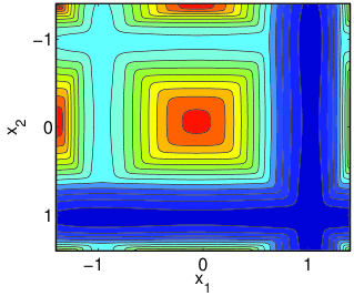
The simple form of (14) or (16) allows for a transparent explanation why these equations are more efficient than the original (1) or (15) at sampling the equilibrium density, and how to choose the artificial temperature $k_{B}\bar{T}=\bar{\beta}^{-1}$ to optimize this efficiency gain. To see this, consider a situation in which the original potential $V(\boldsymbol{x})$ has a minimum of energy at $\boldsymbol{x}_{m}$. Then the mixture potential $U(\boldsymbol{x}_{1},\boldsymbol{x}_{2})$ has a minimum at $(\boldsymbol{x}_{m},\boldsymbol{x}_{m})$, with two channels connected to it along which this potential is a scaled down version of the original one, see the top panel of Fig. 1 for an illustration. Indeed, if the artificial temperature in (14) is much higher than the physical one, $\bar{\beta}\ll\beta$, then in the channel where $\boldsymbol{x}_{2}\approx\boldsymbol{x}_{m}$ we have $U(\boldsymbol{x}_{1},\boldsymbol{x}_{m})\approx\beta^{-1}\bar{\beta}V(\boldsymbol{x}_{1})+V(\boldsymbol{x}_{m})$ in the region where $V(\boldsymbol{x}_{1})>V(\boldsymbol{x}_{m})$, and similarly in the channel where $\boldsymbol{x}_{1}\approx\boldsymbol{x}_{m}$. Thus, along these channels, the equation for $\boldsymbol{x}_{1}$ in (16) can be approximated locally by

$$\begin{cases}\dot{\boldsymbol{x}}_{1}=m^{-1}\boldsymbol{p}_{1},\\ \dot{\boldsymbol{p}}_{1}=\beta^{-1}\bar{\beta}\boldsymbol{f}(\boldsymbol{x}_{1})-\gamma\boldsymbol{p}_{1}+\sqrt{2\gamma m\beta^{-1}}\,\boldsymbol{\eta}_{1},\end{cases}$$ (17)

and similarly for $\boldsymbol{x}_{2}$. (17) is like the original Langevin equation (15) except that the force has been multiplied by a factor $\beta^{-1}\bar{\beta}\ll 1$, meaning the energy barriers have been lowered by this same factor along the channels. In essence, by remaining close to a minimum of the energy, each replica helps the other to surmount barriers and explore the landscape towards other minima, and this is what accelerates the sampling. Note however that, while a replica moves fast along a channel, its weight in the estimator (7) is close zero whereas the one of the replica that hovers near $\boldsymbol{x}_{m}$ is close to one. Indeed when $\boldsymbol{x}_{1}$ moves and $\boldsymbol{x}_{2}\approx\boldsymbol{x}_{m}$, we have $\omega_{\beta,\bar{\beta}}(\boldsymbol{x}_{1},\boldsymbol{x}_{m})\approx 0$ and $\omega_{\bar{\beta},\beta}(\boldsymbol{x}_{1},\boldsymbol{x}_{m})\approx 1$, and similarly when $\boldsymbol{x}_{2}$ moves and $\boldsymbol{x}_{1}\approx\boldsymbol{x}_{m}$. Thus we really need both replica to move in succession, with one of them hovering near a minimum while the other explores the landscape and vice-versa, to achieve proper sampling.

Concerning the choice of temperature, the form of (17) suggests that the optimal $k_{B}\bar{T}=\bar{\beta}^{-1}$ to pick is the highest energy barrier that the system needs to surmount to explore its landscape: at lower values of $k_{B}\bar{T}$, crossing this barrier is still a rare event, and at higher values, we start to blur the sampling by having the system visit regions of too high energies. As we illustrate next on examples, this intuition is correct, except that entropic effects also play an important role in high dimension and may slow down the sampling unless additional replicas with temperatures between $k_{B}T$ and $k_{B}\bar{T}$ are introduced (as will be done in Sec. VI).

To test (14) and (16) and verify the results above, we first consider a system with potential

$$V(x)=(1-x^{2})^{2}-\tfrac{1}{4}x$$ (18)

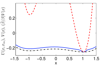
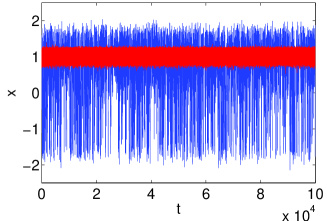
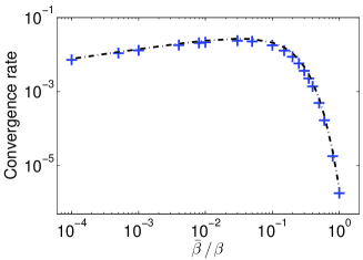
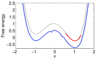
The mixture potential (12) associated with this $V(\boldsymbol{x})$ is plotted in the top panel of Fig. 1, which clearly shows the two channels mentioned before. The Bottom panel of Fig. 1 shows a slice of the mixture potential along one of the channels and compares it with $V(x)$ and its scaled-down version $\beta^{-1}\bar{\beta}V(x)$ when $\beta=25$ (meaning that $k_{B}T=0.04$ and the energy barrier to escape the shallow well is about $20k_{B}T$ at this physical temperature) and $\bar{\beta}=0.8$. The top panel of Fig. 2 shows the times series of the original (1) and the modified (14) for these parameters values. While the solution of (1) is stuck in one well, that of (14) explores the two wells efficiently. The middle panel of Fig. 2 shows the convergence rate of (14) (estimated from the autocorrelation function of the position) as a function of $\bar{\beta}$ and compares it to the analytical estimate of the rate obtained from (17) in the high friction limit. This convergence rate reaches a maximum when $\bar{\beta}=\Delta V^{-1}\approx 0.8$, consistent with the prediction from (17). Finally the bottom panel Fig. 2 shows the free energy reconstructed using (14) with $\bar{\beta}=0.8$ compared to the one obtained from the original (1) with $\beta=25$.

Figure 1: Top panel: The mixture potential (12) for the potential (18) clearly showing the two channel (in dark blue) connected to the minimum. Bottom panel: A slice of the potential along one of the channel (blue solid curve), compared with the original potential $V$ (red dashed curve) and its scaled-down version $(\bar{\beta}/\beta)V$ (black dash-dotted curve).

Figure 2: Replica exchange overdamped dynamics for $V(x)=(x^{2}-1)^{2}-\frac{1}{4}x$. The physical temperature is $T=\beta^{-1}=0.04$ and the auxiliary high temperature is chosen to be $\bar{T}=\bar{\beta}^{-1}=1.25$, the barrier size. The simulation time is $T_{\mathrm{tot}}=10^{5}$ with time step $\mathrm{d}t=0.025$. Top panel: A typical trajectory (blue) of $x_{1}(t)$ of the system (14) hops between both wells frequently, while a typical trajectory (red) under the physical temperature will stay in one of the two wells, as the transition is very rare. Middle panel: The convergence rate of the REMD for overdamped dynamics (14) with $\beta=25$ and different choices of $\bar{\beta}$. The blue solid crosses show the numerical result, the black dash-dotted curve is the estimate obtained from (17) in the high friction limit. Bottom panel: The exact free energy (gray solid curves), that estimated by (14) (blue solid curve) and that estimated by (1) (red solid curve, shifted up by $0.1$ to better illustrate the results).

V The impact of dimensionality and the need for more than two temperatures

As mentioned in Sec. IV, in high dimension entropic effects start to matter and slow down convergence unless more than two temperature are used. To analyze the impact of the dimensionality consider a system with $D$ dimensions moving on the following potential

$$V(x_{0},x_{1},\ldots,x_{D-1})=(1-x_{0}^{2})^{2}-\frac{1}{4}x_{0}+\sum_{j=1}^{D-1}\frac{1}{2}\lambda_{j}x_{j}^{2}$$ (19)

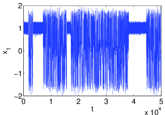
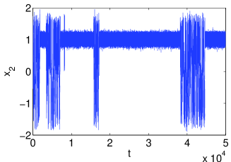
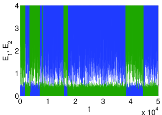
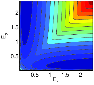
where $\lambda_{1},\lambda_{2},\ldots,\lambda_{D-1}$ are parameters controlling the curvature of the potential in the $x_{1},x_{2},\ldots,x_{D-1}$ directions. In the original equation (15), the dynamics in the $D$ directions are independent, but this is no longer the case for the limiting equation (16) over the mixture potential. When the dimensionality is large, $D\gg 1$, it has the effect that the replica moving in the channel by (17) seldom comes close to a local minimum of the potential because the basin around this minimum is quite wide; at the same time, it has to come close enough to one such minimum to allow the other replica to starts moving in a channel. As can be seen in Fig. 3, this introduces an additional slow time scale in the system when $D$ is large, which is related to the presence of an entropic barrier in the mixture potential. This is shown in Fig. 4 by plotting the free energy $G(E_{1},E_{2})$ of the mixture potential $U(\boldsymbol{x}_{1},\boldsymbol{x}_{2})$ by using the potential energies of the two replica as collective variables:

$$G(E_{1},E_{2}) =-k_{B}T\ln\int_{\mathbb{R}^{3n}\times\mathbb{R}^{3n}}e^{-\beta U(\boldsymbol{x}_{1},\boldsymbol{x}_{2})}$$ (20)

$$\times\delta(V(\boldsymbol{x}_{1})-E_{1})\delta(V(\boldsymbol{x}_{2})-E_{2})\,\mathrm{d}\boldsymbol{x}_{1}\,\mathrm{d}\boldsymbol{x}_{2}$$

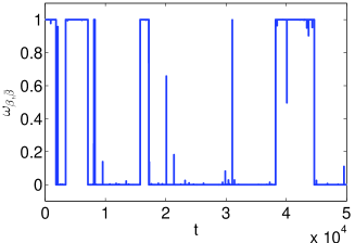
Figure 3: Replica exchange dynamics (14) for the potential (19) with $D=10$, $\beta=25$ and $\bar{\beta}=1$. Top two panels: Typical trajectories of $x_{0}$ for the two replica. Middle panel: Typical trajectories of energies for the two replica. Bottom panel: Corresponding weight factor $\omega_{\beta,\bar{\beta}}$ as a function of $t$. The system switches between the two channels as $\omega_{\beta,\bar{\beta}}$ switches value between $0$ and $1$. This introduces an additional slow time scale to the system.

Figure 4: The mixture potential plotted using the energies of the two replica as coarse grained variables. The entropic barrier at $E_{1}=E_{2}$ introduces a slow time scale for switching between channels.

We can estimate the additional slow time scale to switch from one channel to the other by calculating the mean time the replica moving by (17) takes to come within a region near the local minimum where its potential energy is about $\tfrac{3n}{2}k_{B}T$ above that of the energy minimum. When this event occurs, the other replica has a chance to go in his channel and start moving instead, since $\tfrac{3n}{2}k_{B}T$ is the typical potential energy of the system under physical temperature $T$ by equipartition of energy. However this event becomes less and less likely as the dimensionality increases because the replica moving by (17) effectively feels the rescaled potential $\beta^{-1}\bar{\beta}V(\boldsymbol{x})$ instead of the original one, and so its potential energy tends to be of order $\tfrac{3n}{2}k_{B}\bar{T}$ rather than $\tfrac{3n}{2}k_{B}T$. Assume that $k_{B}T=\beta^{-1}$ is low enough that we can take a quadratic approximation of the potential near the local minimum, $V(\boldsymbol{x})\approx V(\boldsymbol{x}_{m})+\tfrac{1}{2}(\boldsymbol{x}-\boldsymbol{x}_{m})^{\mathrm{T}}H(\boldsymbol{x}-\boldsymbol{x}_{m})$. The region that the moving replica needs to hit is bounded by the ellipsoid defined by $\tfrac{1}{2}(\boldsymbol{x}-\boldsymbol{x}_{m})^{\mathrm{T}}H(\boldsymbol{x}-\boldsymbol{x}_{m})=\tfrac{3n}{2}k_{B}T$, and we can use transition state theory to estimate the mean frequency at which the system governed by (17) hits this ellipsoid:

$$\nu=(\det H)^{1/2}(2\pi)^{D/2}\sqrt{2/\pi\beta}\biggl{(}\frac{\bar{\beta}}{\beta}\biggr{)}^{D/2}e^{-\bar{\beta}/\beta}\sigma_{H},$$ (21)

where $D=3n$ and $\sigma_{H}$ is the surface area of the ellipsoid $\tfrac{1}{2}\boldsymbol{x}^{\mathrm{T}}H\boldsymbol{x}=1$. Using Carlson’s bound Carlson (1966) for $\sigma_{H}$, we obtain an upper bound

$$\nu\leq\frac{D^{1/2}(2\pi)^{D}}{\Gamma((D+1)/2)}\sqrt{\frac{\Lambda}{\pi\beta}}\biggl{(}\frac{\bar{\beta}}{\beta}\biggr{)}^{D/2},$$ (22)

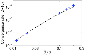
where $\Lambda$ is the mean curvature of the potential well. The frequency $\nu$ also gives the mean rate at which the two replica switch from moving fast in the channels or remaining trapped near a minimum. Fig. 5 shows the convergence rate of (14) (estimated from the autocorrelation function of the position) for the potential (19) and shows that this rate is indeed dominated by the mean hitting frequency in (22) when $D$ is large ($D=10$ for the results reported in the figure: $D=3n$ for system (15)). To avoid this slowing down effect, more than two temperature must be used, as explained next.

Figure 5: The convergence rate of the REMD for overdamped dynamics with $D=10$ with $\beta=25$ and different choices of $\bar{\beta}$. The blue solid crosses show the numerical result, the black dash-dotted curve is the upper bound (22) obtained from the inverse of mean hitting time of (17) to a small ball around the local minimum of the potential where the energy is of order $k_{B}T$ from that of this minimum

VI Using multiple temperatures

The discussion in Sec. V indicates the need to take more than two temperatures to accelerate convergence for high dimensional systems. If we use $N$ temperatures from the physical $k_{B}T$ to the optimal $k_{B}\bar{T}$, i.e.

$$\beta_{1}\equiv\beta=\frac{1}{k_{B}T}>\beta_{2}>\cdots>\beta_{N}\equiv\bar{\beta}=\frac{1}{k_{B}\bar{T}},$$ (23)

then (12) generalizes into the following mixture potential constructed by symmetrization over the $N!$ permutations of the $N$ temperatures among the $N$ replicas:

$$U(\boldsymbol{x}_{1},\ldots,\boldsymbol{x}_{N})$$ (24)

$$=-k_{B}T\ln\sum_{\sigma}e^{-\beta_{1}V(\boldsymbol{x}_{\sigma(1)})\cdots-\beta_{N}V(\boldsymbol{x}_{\sigma(N)})}$$

where $\sum_{\sigma}$ denotes the sum over all the permutations $\sigma$ of the indices $\{1,2,\ldots,N\}$. In turn, the system (16) becomes

$$\begin{cases}\dot{\boldsymbol{x}}_{j}=m^{-1}\boldsymbol{p}_{j},\\ \dot{\boldsymbol{p}}_{j}=R_{j}\boldsymbol{f}(\boldsymbol{x}_{j})-\gamma\boldsymbol{p}_{j}+\sqrt{2\gamma m\beta_{j}^{-1}}\,\boldsymbol{\eta}_{j},\end{cases}$$ (25)

where $j=1,\ldots,N$ and $\boldsymbol{\eta}_{j}$ are independent white-noises. Here we defined

$$R_{j}=\beta^{-1}\sum_{\sigma}\beta_{\sigma(j)}\omega_{\sigma(1),\ldots,\sigma(N)}(\boldsymbol{x}_{1},\dots,\boldsymbol{x}_{N})$$ (26)

with

$$\omega_{\sigma(1),\ldots,\sigma(N)}(\boldsymbol{x}_{1},\dots,\boldsymbol{x}_{N})$$ (27)

$$\quad=\frac{e^{-\beta_{1}V(\boldsymbol{x}_{\sigma(1)})\cdots-\beta_{N}V(\boldsymbol{x}_{\sigma(N)})}}{\sum_{\sigma^{\prime}}e^{-\beta_{1}V(\boldsymbol{x}_{\sigma^{\prime}(1)})\cdots-\beta_{N}V(\boldsymbol{x}_{\sigma^{\prime}(N)})}}$$

If the temperatures in (23) are far apart, then at any given time there typically is one specific permutation $\sigma^{*}$ such that $\omega_{\sigma^{*}(1),\ldots,\sigma^{*}(N)}(\boldsymbol{x}_{1},\dots,\boldsymbol{x}_{N})\approx 1$ whereas these weights are close to zero for all the other permutations. This is the multiple replicas equivalent of the slow switch phenomenon between $\omega_{\beta,\bar{\beta}}$ and $\omega_{\bar{\beta},\beta}$ being alternatively 1 or 0 that we observed in Sec. V with two replicas and it means that

$$R_{j}\approx\beta^{-1}\beta_{\sigma^{*}(j)}\leq 1,$$ (28)

i.e. all the forces in (25) are rescaled by factors that are less or equal to 1. Up to relabeling of the replicas, we can always assume temporarily that $\sigma^{*}(j)=j$, meaning that the factors $R_{j}$ are ordered as $1=R_{1}>R_{2}>\cdots>R_{N}$. The most likely way for these factors to change order is that one of the $j$-th replica hits a small ball where its potential energy becomes of order $k_{B}T_{j-1}$: again this is the multiple replica equivalent of the channel switching process that we observed in Sec. V with two replicas. When this process occurs, the permutation $\sigma^{*}$ for which the weight is approximately one becomes that in which the indices $j-1$ and $j$ have been permuted. The frequencies $\nu_{j}$ at which these swaps occur can be estimated as in Sec. V (compare (22)):

$$\nu_{j}\leq\frac{D^{1/2}(2\pi)^{D}}{\Gamma((D+1)/2)}\sqrt{\frac{\Lambda}{\pi\beta_{j}}}\biggl{(}\frac{\beta_{j+1}}{\beta_{j}}\biggr{)}^{D/2}.$$ (29)

This estimate suggests that we should take a geometric progression of temperatures in which their successive ratio is kept constant in order for all the $\nu_{j}$ (and hence the time scales of channel switching) to be of the same order:

$$\frac{\beta_{j+1}}{\beta_{j}}=\left(\frac{\bar{\beta}}{\beta}\right)^{1/(N-1)}\qquad j=1,\ldots,N-1$$ (30)

This choice agrees with the conventional choice in the literature (see e.g. discussions in Refs. [Kofke, 2002; Rathore et al., 2005; Rosta and Hummer, 2009; Denschlag et al., 2009]) but gives a different perspective on it.

The discussion above also indicates how many replicas should be used. Specifically, one should aim at eliminating the slow time scale of channel switching by taking the successive temperature sufficiently close together: clearly, in (30) the higher $N$, the closer to 1 the ratio $\beta_{j+1}/\beta_{j}$ becomes even if $\bar{\beta}/\beta$ is very small. However, this may require taking many replicas, which in practice poses a difficulty for our approach because the number $N!$ of terms involved in the weight (27) grows very fast with $N$.

Several strategies can be used to alleviate this problem. For example, one can decrease the effective dimensionality of the system by only raising the temperature of a few important degrees of freedom in the system. This idea was implemented e.g. in Ref. Liu et al., 2005 for biomolecular simulations in solvent.

Another strategy, originally proposed in Ref. Plattner et al., 2011 is to perform partial swapping. Instead of symmetrizing the potential over the whole set of the $N$ replicas associated with the $N$ temperatures, the idea is to divide them into several groups consisting a moderate number of replicas. In each group, a mixture potential like (24) with $N$ replaced by the number of replica in the group is used to evolve the system. To fully mix the temperatures, multiple partitions are used to distribute the replica in the different groups and the temperatures in the groups of each partition are reassigned dynamically. While none of partition by itself will fully mix every replica, combining these partitions together permits to achieve a full mixture of the $N$ replica.

To simplify the presentation of the algorithm, let us consider the case $N=3$, with the two partitions given by $A=(12)(3)$ and $B=(1)(23)$; the extension to the general case is straightforward. We denote $\alpha_{i}(t)$ the temperature assigned to the $i$-th replica, which takes value in $\beta_{1}=\beta,\beta_{2}$ and $\beta_{3}=\bar{\beta}$. At the start of the simulation, we set $\alpha_{i}(0)=\beta_{i}$. We then evolve the system using the two partitions $A$ and $B$ alternatively and dynamically reassign the temperatures as we switch between the two partitions. This is done by repeating the following procedures which evolve the system from time $t$ to time $t+2\Delta t$:

1. Evolve the system using partition $A$ from $t$ to $t+\Delta t$: The group of replica $1$ and $2$ is evolved using (16) with the mixture potential

   $$U_{\alpha_{1}(t),\alpha_{2}(t)}(\boldsymbol{x}_{1},\boldsymbol{x}_{2})=-\beta_{1}^{-1}\ln(e^{-\alpha_{1}(t)V(\boldsymbol{x}_{1})-\alpha_{2}(t)V(\boldsymbol{x}_{2})}\\ +e^{-\alpha_{2}(t)V(\boldsymbol{x}_{1})-\alpha_{1}(t)V(\boldsymbol{x}_{2})}).$$ (31)

   As the other group only consists of replica $3$, it is evolved under scaled potential $\alpha_{3}(t)\beta_{1}^{-1}V(\boldsymbol{x}_{3})$ which is just the mixture potential with only one replica.

2. At time $t+\Delta t$, reassign the temperatures within each group in partition $A$: We set

   $$\begin{cases}\alpha_{1}(t+\Delta t)=\alpha_{1}(t)\\ \alpha_{2}(t+\Delta t)=\alpha_{2}(t)\end{cases}$$

   with probability $\omega_{\alpha_{1}(t),\alpha_{2}(t)}(\boldsymbol{x}_{1},\boldsymbol{x}_{2})$ and

   $$\begin{cases}\alpha_{1}(t+\Delta t)=\alpha_{2}(t)\\ \alpha_{2}(t+\Delta t)=\alpha_{1}(t)\end{cases}$$

   with probability $\omega_{\alpha_{2}(t),\alpha_{1}(t)}(\boldsymbol{x}_{1},\boldsymbol{x}_{2})=1-\omega_{\alpha_{1}(t),\alpha_{2}(t)}(\boldsymbol{x}_{1},\boldsymbol{x}_{2})$. Hence, one particular assignment is chosen for each group from the symmetrization.

3. Repeat the above two steps to evolve partition $B$ from $t+\Delta t$ to $t+2\Delta t$. The replica $1$ is evolved under the potential $\alpha_{1}(t+\Delta t)\beta_{1}^{-1}V(\boldsymbol{x}_{1})$. The group of replica $2$ and $3$ is evolved with the mixture potential

   $$U_{\alpha_{2}(t+\Delta t),\alpha_{3}(t+\Delta t)} (\boldsymbol{x}_{2},\boldsymbol{x}_{3})=$$ (32)

   $$-\beta_{1}^{-1}\ln( e^{-\alpha_{2}(t+\Delta t)V(\boldsymbol{x}_{2})-\alpha_{3}(t+\Delta t)V(\boldsymbol{x}_{3})}$$

   $$+ e^{-\alpha_{2}(t+\Delta t)V(\boldsymbol{x}_{3})-\alpha_{3}(t+\Delta t)V(\boldsymbol{x}_{2})}).$$

4. At time $t+2\Delta t$, reassign the temperatures within each group in partition $B$: We set

   $$\begin{cases}\alpha_{2}(t+2\Delta t)=\alpha_{2}(t+\Delta t)\\ \alpha_{3}(t+2\Delta t)=\alpha_{3}(t+\Delta t)\end{cases}$$

   with probability $\omega_{\alpha_{2}(t+\Delta t),\alpha_{3}(t+\Delta t)}(\boldsymbol{x}_{2},\boldsymbol{x}_{3})$ and

   $$\begin{cases}\alpha_{2}(t+2\Delta t)=\alpha_{3}(t+\Delta t)\\ \alpha_{3}(t+2\Delta t)=\alpha_{2}(t+\Delta t)\end{cases}$$

   with probability $\omega_{\alpha_{3}(t+\Delta t),\alpha_{2}(t+\Delta t)}(\boldsymbol{x}_{2},\boldsymbol{x}_{3})=1-\omega_{\alpha_{2}(t+\Delta t),\alpha_{3}(t+\Delta t)}(\boldsymbol{x}_{2},\boldsymbol{x}_{3})$.

This partial mixing strategy can be viewed as a generalization of the usual replica exchange molecular dynamics in which several replica are grouped together and evolved under a mixture potential. The parameter $\Delta t$ is analogous to the inverse of swapping attempt frequency in the conventional replica exchange. Therefore, it is more advantageous to take a small $\Delta t$ to increase the swapping frequency. In practice, we can take $\Delta t$ equal to the time-step used in the MD simulations.

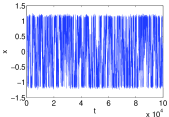
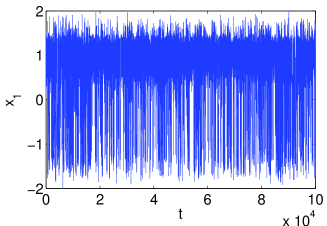
The performance of the partial swapping algorithm is illustrated in Fig. 6 with three temperatures $\beta_{1}=25$, $\beta_{2}=5$ and $\beta_{3}=1$. Compared with Fig. 3 the slow time scale of switching between channels is now removed due to introduction of an intermediate temperature.

Figure 6: Partial swapping REMD for the potential (19) with $\beta_{1}=25$, $\beta_{2}=5$ and $\beta_{3}=1$. A typical trajectory for one of the replica is plotted.

VII Lennard-Jones example

Finally, to test the performance of our algorithm on a more realistic example, we apply (16) to the model system proposed in Ref. Dellago et al., 1999. This system consists of $N$ two-dimensional particles in a periodic box with side length $l$. All particles have the same mass $m$, and they interact with each other with the Weeks-Chandler-Anderson potential defined as

$$V_{\text{WCA}}(r)=4\epsilon\Bigl{(}(\sigma/r)^{12}-(\sigma/r)^{6}\Bigr{)}+\epsilon,$$ (33)

if $r\leq r_{\text{WCA}}=2^{1/6}\sigma$, and $V_{\text{WCA}}(r)=0$ otherwise, except for a pair of particles, which interact via a double well potential

$$V_{\text{dW}}(r)=h\Bigl{(}1-\frac{(r-r_{\text{WCA}}-w)^{2}}{w^{2}}\Bigr{)}^{2}.$$ (34)

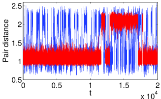
We take $N=16$, $l=4.4$, $\sigma=1$, $h=1$, $w=0.5$, and $\epsilon=1$ in the simulation. The physical temperature is $T=0.2$, and for this system, it turns out that it suffices to use two temperatures with the auxiliary high temperature chosen to be $\bar{T}=1$. The quantity of interest is the free energy associated with the distance of the pair of particles interacting via the double well potential. The trajectories of the pair distance is shown in Figure 7, compared to a direct molecular dynamics simulation. While the original dynamics exhibits metastability in switching between the compressed and elongated states of the pair distance, it is observed that the dynamics on the mixture potential efficiently sample the configurational space.

Figure 7: Molecular dynamics example. A typical trajectory of the pair distance between the pair of particles interact with double well potential in the molecular dynamics simulation under physical temperature (red) stays in the compressed and elongated states for a long time, while the trajectory under the dynamics (16) exhibits frequent transitions between the compressed and elongated states.

VIII Generalizations

We have used the mixture potential to mix two temperatures in the above discussion but the idea extends naturally to mixture based on other parameters. For example, we can mix the original potential with a modified one in which the barriers between metastable regions is reduced. Such a modified potential may come from e.g. spatial warping Zhu et al. (2002) or solute tempering Liu et al. (2005). If we denote by $\bar{V}$ the auxiliary modified potential, the dynamics is given by

$$\begin{cases}\dot{\boldsymbol{x}}_{1}=m^{-1}\boldsymbol{p}_{1},\\ \dot{\boldsymbol{p}}_{1}=(\omega_{V,\bar{V}}\boldsymbol{f}(\boldsymbol{x}_{1})+\omega_{\bar{V},V}\bar{\boldsymbol{f}}(\boldsymbol{x}_{1}))\\ \hskip 80.00012pt-\gamma\boldsymbol{p}_{1}+\sqrt{2\gamma\beta^{-1}m}\ \boldsymbol{\eta}_{1}(t),\\ \dot{\boldsymbol{x}}_{2}=m^{-1}\boldsymbol{p}_{2},\\ \dot{\boldsymbol{p}}_{2}=(\omega_{V,\bar{V}}\bar{\boldsymbol{f}}(\boldsymbol{x}_{2})+\omega_{\bar{V},V}\boldsymbol{f}(\boldsymbol{x}_{2}))\\ \hskip 80.00012pt-\gamma\boldsymbol{p}_{2}+\sqrt{2\gamma\beta^{-1}m}\ \boldsymbol{\eta}_{2}(t),\end{cases}$$ (35)

where $\boldsymbol{f}$ and $\boldsymbol{\bar{f}}$ are the forces corresponding to the potentials $V$ and $\bar{V}$ respectively, and the weight $\omega_{V,\bar{V}}$ is given by

$$\omega_{V,\bar{V}}(\boldsymbol{x}_{1},\boldsymbol{x}_{2})=\frac{e^{-\beta V(\boldsymbol{x}_{1})-\beta\bar{V}(\boldsymbol{x}_{2})}}{e^{-\beta V(\boldsymbol{x}_{1})-\beta\bar{V}(\boldsymbol{x}_{2})}+e^{-\beta\bar{V}(\boldsymbol{x}_{1})-\beta V(\boldsymbol{x}_{2})}}$$ (36)

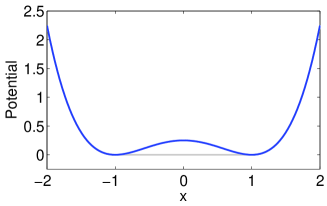
and similarly for $\omega_{\bar{V},V}$. The performance (35) is illustrated on a double-well example in Figure 8: here the modified potential $\bar{V}$ is simply the original one in which we have removed the barrier.

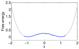
Figure 8: Numerical results for the dynamics (35). Top panel: The physical double well potential $V(x)=(x^{2}-1)^{2}/4$ (blue) and the auxiliary potential $\bar{V}$ (gray) where the barrier is removed. The other parameters in the model are $m=1$, $\gamma=1$, $\beta=100$, $T_{\mathrm{tot}}=1e5$ and $\mathrm{d}t=0.1$. Middle panel: A typical trajectory of $X_{1}(t)$ of the dynamics (35). Since $\bar{V}$ has no barrier, the dynamics efficiently explore the region between the two local minima of the original potential. Bottom panel: Comparison of the estimated (blue) and exact (gray) free energies.

IX Concluding remarks

We have presented a natural reformulation of the infinite swapping limit of REMD that enables a simple implementation in which forces in standard MD simulations are rescaled by factors involving the energies of all the replica. This reformulation is equivalent to having the system evolve over a mixture potential, and thereby permits to analyze the efficiency of REMD by using familiar tools like Arrhenius formula and transition state theory. It also gives us insights on how to choose an optimal sequence of temperatures in REMD. Finally, it leads naturally to generalizations in which the mixture potential is constructed by varying parameters in the potential other than the temperature, like for example those used in spatial warping Zhu et al. (2002) or solute tempering Liu et al. (2005).

Appendix A Dynamics based on Mixture Hamiltonian

The formulation of the method presented in text involves a mixture potential, but this mixing can be done on the level of Hamiltonians too. We briefly describe this alternative in this appendix. Consider a mixture Hamiltonian of two replica

$$H(\boldsymbol{x}_{1},\boldsymbol{p}_{1},\boldsymbol{x}_{2},\boldsymbol{p}_{2})=-k_{B}T\ln\left(e^{-\beta E_{1}-\bar{\beta}E_{2}}+e^{-\bar{\beta}E_{1}-\beta E_{2}}\right).$$ (37)

where $E_{1}=E(\boldsymbol{x}_{1},\boldsymbol{p}_{1})$ and $E_{2}=E(\boldsymbol{x}_{2},\boldsymbol{p}_{2})$. The equations of motion associated with this Hamiltonian are

$$\begin{cases}\dot{\boldsymbol{x}}_{1}=m^{-1}(\omega_{\beta,\bar{\beta}}+\beta^{-1}\bar{\beta}\omega_{\bar{\beta},\beta})\boldsymbol{p}_{1},\\ \dot{\boldsymbol{p}}_{1}=(\omega_{\beta,\bar{\beta}}+\beta^{-1}\bar{\beta}\omega_{\bar{\beta},\beta})\boldsymbol{f}(\boldsymbol{x}_{1})\\ \hskip 80.00012pt-\gamma\boldsymbol{p}_{1}+\sqrt{2\gamma m\beta^{-1}}\,\boldsymbol{\eta}_{1},\\ \dot{\boldsymbol{x}}_{2}=m^{-1}(\omega_{\bar{\beta},\beta}+\beta^{-1}\bar{\beta}\omega_{\beta,\bar{\beta}})\boldsymbol{p}_{2},\\ \dot{\boldsymbol{p}}_{2}=(\omega_{\bar{\beta},\beta}+\beta^{-1}\bar{\beta}\omega_{\beta,\bar{\beta}})\boldsymbol{f}(\boldsymbol{x}_{2})\\ \hskip 80.00012pt-\gamma\boldsymbol{p}_{2}+\sqrt{2\gamma m\beta^{-1}}\,\boldsymbol{\eta}_{2}.\end{cases}$$ (38)

where the weight functions $\omega_{\beta,\bar{\beta}}$ are given by

$$\omega_{\beta,\bar{\beta}}(\boldsymbol{x}_{1},\boldsymbol{p}_{1},\boldsymbol{x}_{2},\boldsymbol{p}_{2})=\frac{e^{-\beta E_{1}-\bar{\beta}E_{2}}}{e^{-\beta E_{1}-\bar{\beta}E_{2}}+e^{-\beta E_{2}-\bar{\beta}E_{1}}}.$$ (39)

Observe that in the mixture Hamiltonian dynamics, both equations for $\boldsymbol{x}$ and $\boldsymbol{p}$ have rescaling terms depending on the weights $\omega_{\beta,\bar{\beta}}$. Thus, compared with (16), the dynamics in (38) mixes together both the kinetic and the potential energies of the two replicas. As a consequence, in high dimension, the switching of $\omega_{\beta,\bar{\beta}}$ from $0$ to $1$ and vice-versa will be further slowed down. This suggests that it is more advantageous to use (16) rather than (38).

References

• Hansmann (1997) U. H. E. Hansmann, Chem. Phys. Lett. 281, 140 (1997).
• Sugita and Okamoto (1999) Y. Sugita and Y. Okamoto, Chem. Phys. Lett. 314, 141 (1999).
• Sugita et al. (2000) Y. Sugita, A. Kitao,  and Y. Okamoto, J. Chem. Phys. 113, 6042 (2000).
• Rao and Caflisch (2003) F. Rao and A. Caflisch, J. Chem. Phys. 119, 4035 (2003).
• Earl and Deem (2005) D. J. Earl and W. Deem, Phys. Chem. Chem. Phys. 7, 3910 (2005).
• Swendsen and Wang (1986) R. H. Swendsen and J.-S. Wang, Phys. Rev. Lett. 57, 2607 (1986).
• Geyer (1991) C. J. Geyer, in Computing Science and Statistics: Proc. 23rd Symposium on the Interface, edited by E. M. Keramidas (Interface Foundation, Fairfax Station, VA, 1991) pp. 156–163.
• Geyer and Thompson (1995) C. J. Geyer and E. Thompson, J. Amer. Statist. Assoc. 90, 909 (1995).
• Hukushima and Nemoto (1996) K. Hukushima and K. Nemoto, J. Phys. Soc. Jpn. 65, 1604 (1996).
• Marinari et al. (1998) E. Marinari, G. Parisi,  and J. J. Ruiz-Lorenzo, in Spin Glasses and Random Fields, edited by A. P. Young (World Scientific, Singapore, 1998) pp. 59–98.
• Tesi et al. (1996) M. C. Tesi, E. J. Janse van Rensburg, E. Orlandini,  and S. G. Whittington, J. Stat. Phys. 82, 155 (1996).
• Sindhikara et al. (2008) D. Sindhikara, Y. Meng,  and A. E. Roitberg, J. Chem. Phys. 128, 024103 (2008).
• Abraham and Gready (2008) M. J. Abraham and J. E. Gready, J. Chem. Theory Comput. 4, 1119 (2008).
• Plattner et al. (2011) N. Plattner, J. D. Doll, P. Dupuis, H. Wang, Y. Liu,  and J. E. Gubernatis, J. Chem. Phys. 135, 134111 (2011).
• Dupuis et al. (2012) P. Dupuis, Y. Liu, N. Plattner,  and J. D. Doll, Multiscale Model. Simul. 10, 986 (2012).
• Carlson (1966) B. C. Carlson, Proc. Amer. Math. Soc. 17, 32 (1966).
• Kofke (2002) D. A. Kofke, J. Chem. Phys. 117, 6911 (2002).
• Rathore et al. (2005) N. Rathore, M. Chopra,  and J. J. de Pablo, J. Chem. Phys. 122, 024111 (2005).
• Rosta and Hummer (2009) E. Rosta and G. Hummer, J. Chem. Phys. 131, 165102 (2009).
• Denschlag et al. (2009) R. Denschlag, M. Lingenheil,  and P. Tavan, Chem. Phys. Lett. 473, 193 (2009).
• Liu et al. (2005) P. Liu, B. Kim, R. A. Friesner,  and B. J. Berne, Proc. Natl. Acad. Sci. USA 102, 13749 (2005).
• Dellago et al. (1999) C. Dellago, P. G. Bolhuis,  and D. Chandler, J. Chem. Phys. 110, 6617 (1999).
• Zhu et al. (2002) Z. Zhu, M. Tuckerman, S. Samuelson,  and G. Martyna, Phys. Rev. Lett. 88, 100201 (2002).