Temperature, gravity and bolometric correction scales
for non-supergiant OB stars††thanks: Based on observations collected at the
Centro Astronómico Hispano Alemán (CAHA) at Calar Alto, operated
jointly by the Max-
Planck Institut für Astronomie and the Instituto de Astrofísica
de Andalucía (CSIC), proposals H2001-2.2-011
and H2005-2.2-016.,††thanks: Based on observations collected at the European Southern
Observatory, Chile, ESO 074.B-0455(A) and from the ESO Archive.,††thanks: Based on spectral data retrieved from the ELODIE archive at
Observatoire de Haute-Provence (OHP).
Abstract
Context. Precise and accurate determinations of the atmospheric parameters effective temperature and surface gravity are mandatory to derive reliable chemical abundances in OB stars. Furthermore, fundamental parameters like distances, masses, radii, luminosities can also be derived from the temperature and gravity of the stars.
Aims. Atmospheric parameters recently determined at high precision with several independent spectroscopic indicators in NLTE, with typical uncertainties of 300 K for temperature and of 0.05 dex for gravity, are employed to calibrate photometric relationships. This is in order to investigate whether a faster tool to estimate atmospheric parameters can be provided.
Methods. Temperatures and gravities of 30 calibrators, i.e. well-studied OB main sequence to giant stars in the solar neighbourhood, are compared to reddening-independent quantities of the Johnson and Strömgren photometric systems, assuming normal reddening. In addition, we examine the spectral and luminosity classification of the star sample and compute bolometric corrections.
Results. Calibrations of temperatures and gravities are proposed for various photometric indices and spectral types. Once the luminosity of the stars is well known, effective temperatures can be determined at a precision of 400 K for luminosity classes III/IV and 800 K for luminosity class V. Furthermore, surface gravities can reach internal uncertainties as low as 0.08 dex when using our calibration to the Johnson -parameter. Similar precision is achieved for gravities derived from the -index and the precision is lower for both atmospheric parameters when using the Strömgren indices and . In contrast, external uncertainties are larger for the Johnson than for the Strömgren calibrations. Our uncertainties are smaller than typical differences among other methods in the literature, reaching values up to 2000 K for temperature and 0.25 dex for gravity, and in extreme cases, 6000 K and 0.4 dex, respectively. A parameter calibration for sub-spectral types is also proposed. Moreover, we present a new bolometric correction relation to temperature based on our empirical data, rather than on synthetic grids.
Conclusions. The photometric calibrations presented here are useful tools to estimate effective temperatures and surface gravities of non-supergiant OB stars in a fast manner. This is also applicable to some single-line spectroscopic binaries, but caution has to be taken for undetected double-lined spectroscopic binaries and single objects with anomalous reddening-law, dubious photometric quantities and/or luminosity classes, for which the systematic uncertainties may increase significantly. We recommend to use these calibrations only as a first step of the parameter estimation, with subsequent refinements based on spectroscopy. A larger sample covering more uniformly the parameter space under consideration will allow refinements to the present calibrations.
Key Words.:
Stars: fundamental parameters, stars: early-type, stars: atmospheres| HD | HR | Name | Sp. T2 | |||||||||||||||
|---|---|---|---|---|---|---|---|---|---|---|---|---|---|---|---|---|---|---|
| mag | mag | mag | mag | mag | mag | mag | mag | K | dex | km s-1 | ||||||||
| 1 | 36591 | 1861 | B1 V | 5.339 | 0.194 | 0.911 | 0.771 | 0.077 | 0.074 | -0.002 | 2.612 | 27000 | 4.12 | 3 | 12 | … | ||
| … | … | … | … | … | … | … | … | 300 | 0.05 | 1 | 1 | … | ||||||
| 2 | 61068 | 2928 | PT Pup | B1 V3,4 | 5.711 | 0.176 | 0.868 | 0.741 | 0.068 | 0.077 | 0.050 | 2.617 | 26300 | 4.15 | 3 | 14 | 20 | |
| 0.015 | 0.010 | 0.015 | 0.017 | 0.003 | 0.001 | 0.002 | 0.003 | 300 | 0.05 | 1 | 2 | 1 | ||||||
| 3 | 63922 | 3055 | B0.2 III4 | 4.106 | 0.185 | 1.010 | 0.877 | 0.051 | 0.043 | -0.078 | 2.591 | 31200 | 3.95 | 8 | 29 | 37 | ||
| 0.005 | 0.007 | 0.000 | 0.005 | 0.006 | 0.004 | 0.002 | 0.005 | 300 | 0.05 | 1 | 4 | 8 | ||||||
| 4 | 74575 | 3468 | Pyx | B1.5 III | 3.679 | 0.183 | 0.875 | 0.743 | 0.063 | 0.066 | 0.050 | 2.604 | 22900 | 3.60 | 5 | 11 | 20 | |
| 0.006 | 0.003 | 0.007 | 0.007 | 0.002 | 0.002 | 0.007 | 0.002 | 300 | 0.05 | 1 | 2 | 1 | ||||||
| 5 | 122980 | 5285 | Cen | B2 V4 | 4.353 | 0.195 | 0.774 | 0.634 | 0.094 | 0.096 | 0.168 | 2.656 | 20800 | 4.22 | 3 | 18 | … | |
| 0.007 | 0.006 | 0.013 | 0.014 | 0.003 | 0.006 | 0.006 | 0.004 | 300 | 0.05 | 1 | 1 | … | ||||||
| 6 | 149438 | 6165 | Sco | B0.2 V | 2.825 | 0.252 | 1.023 | 0.842 | 0.093 | 0.039 | -0.090 | 2.601 | 32000 | 4.30 | 5 | 4 | 4 | |
| 0.009 | 0.007 | 0.013 | 0.014 | 0.008 | 0.015 | 0.023 | 0.007 | 300 | 0.05 | 1 | 1 | 1 | ||||||
| 7 | 886 | 39 | Peg | B2 IV | 2.834 | 0.226 | 0.862 | 0.699 | 0.107 | 0.093 | 0.116 | 2.627 | 22000 | 3.95 | 2 | 9 | 8 | |
| 0.015 | 0.012 | 0.012 | 0.015 | 0.003 | 0.001 | 0.000 | 0.003 | 400 | 0.05 | 1 | 2 | 2 | ||||||
| 8 | 29248 | 1463 | Eri | B1.5 IV3,4 | 3.930 | 0.210 | 0.879 | 0.728 | 0.076 | 0.068 | 0.072 | 2.610 | 22000 | 3.85 | 6 | 26 | 15 | |
| 0.023 | 0.009 | 0.007 | 0.010 | 0.000 | 0.004 | 0.010 | 0.002 | 250 | 0.05 | 1 | 2 | 5 | ||||||
| 9 | 35299 | 1781 | B1.5 V | 5.694 | 0.210 | 0.874 | 0.723 | 0.094 | 0.088 | 0.057 | 2.631 | 23500 | 4.20 | 0 | 8 | … | ||
| 0.010 | 0.007 | 0.011 | 0.012 | 0.002 | 0.004 | 0.005 | 0.003 | 300 | 0.05 | 1 | 1 | … | ||||||
| 10 | 35708 | 1810 | Tau | B2 V3,4 | 4.875 | 0.145 | 0.768 | 0.664 | 0.058 | 0.090 | 0.151 | 2.642 | 20700 | 4.15 | 2 | 25 | 17 | |
| 0.012 | 0.006 | 0.005 | 0.007 | … | … | … | … | 200 | 0.07 | 1 | 2 | 5 | ||||||
| 11 | 36512 | 1855 | Ori | B0 V | 4.618 | 0.264 | 1.068 | 0.878 | 0.112 | 0.061 | -0.095 | 2.597 | 33400 | 4.30 | 4 | 20 | 10 | |
| 0.013 | 0.007 | 0.008 | 0.009 | 0.005 | 0.000 | 0.004 | 0.003 | 200 | 0.05 | 1 | 2 | 5 | ||||||
| 12 | 36822 | 1876 | Ori | B0.5 III4 | 4.408 | 0.162 | 0.965 | 0.848 | 0.037 | 0.026 | -0.062 | 2.602 | 30000 | 4.05 | 8 | 28 | 18 | |
| 0.006 | 0.013 | 0.013 | 0.016 | … | … | … | … | 300 | 0.10 | 1 | 2 | 5 | ||||||
| 13 | 36960 | 1887 | B0.7 V4 | 4.785 | 0.250 | 1.015 | 0.830 | 0.106 | 0.072 | -0.056 | 2.600 | 29000 | 4.10 | 4 | 28 | 20 | ||
| 0.007 | 0.010 | 0.016 | 0.018 | 0.004 | 0.002 | 0.003 | 0.003 | 300 | 0.07 | 1 | 3 | 7 | ||||||
| 14 | 205021 | 8238 | Cep | B1 IV | 3.233 | 0.222 | 0.952 | 0.792 | 0.092 | 0.066 | 0.010 | 2.605 | 27000 | 4.05 | 4 | 28 | 20 | |
| 0.014 | 0.006 | 0.011 | 0.012 | 0.002 | 0.003 | 0.006 | 0.003 | 450 | 0.05 | 1 | 3 | 7 | ||||||
| 15 | 209008 | 8385 | 18 Peg | B3 III | 5.995 | 0.120 | 0.568 | 0.482 | 0.035 | 0.081 | 0.411 | 2.660 | 15800 | 3.75 | 4 | 15 | 10 | |
| 0.008 | 0.014 | 0.013 | 0.016 | 0.000 | 0.003 | 0.002 | 0.003 | 200 | 0.05 | 1 | 3 | 3 | ||||||
| 16 | 216916 | 8725 | EN Lac | B1.5 IV4 | 5.587 | 0.144 | 0.836 | 0.732 | 0.047 | 0.066 | 0.092 | 2.629 | 23000 | 3.95 | 0 | 12 | … | |
| 0.015 | 0.008 | 0.007 | 0.009 | 0.004 | 0.003 | 0.007 | 0.007 | 200 | 0.05 | 1 | 1 | … | ||||||
| 17 | 3360 | 153 | Cas | B2 IV | 3.661 | 0.196 | 0.849 | 0.708 | 0.090 | 0.087 | 0.134 | 2.627 | 20750 | 3.80 | 2 | 20 | 12 | |
| 0.017 | 0.006 | 0.024 | 0.024 | 0.000 | 0.000 | 0.000 | 0.005 | 200 | 0.05 | 1 | 2 | 5 | ||||||
| 18 | 16582 | 779 | Cet | B2 IV | 4.067 | 0.219 | 0.850 | 0.692 | 0.099 | 0.091 | 0.102 | 2.616 | 21250 | 3.80 | 2 | 15 | 10 | |
| 0.007 | 0.008 | 0.014 | 0.015 | 0.001 | 0.002 | 0.008 | 0.004 | 400 | 0.05 | 1 | 2 | 5 | ||||||
| 19 | 34816 | 1756 | Lep | B0.5 V3 | 4.286 | 0.273 | 1.010 | 0.813 | 0.110 | 0.073 | -0.061 | 2.602 | 30400 | 4.30 | 4 | 30 | 20 | |
| 0.005 | 0.015 | 0.005 | 0.012 | 0.001 | 0.004 | 0.003 | 0.002 | 300 | 0.05 | 1 | 2 | 7 | ||||||
| 20 | 160762 | 6588 | Her | B3 IV | 3.800 | 0.179 | 0.702 | 0.573 | 0.065 | 0.079 | 0.292 | 2.661 | 17500 | 3.80 | 1 | 6 | … | |
| 0.000 | 0.003 | 0.010 | 0.010 | 0.002 | 0.004 | 0.004 | 0.001 | 200 | 0.05 | 1 | 1 | … | ||||||
| 21 | 370205 | 1893 | 1 Ori A | B0.5 V | 6.720 | 0.000 | 0.860 | 0.860 | 0.092 | 0.029 | -0.048 | 2.573 | 30700 | 4.30 | 0 | 45 | 20 | |
| … | … | … | … | 0.002 | 0.003 | 0.008 | 0.022 | 300 | 0.07 | 1 | 6 | 10 | ||||||
| 22 | 370425 | 2 Ori B | B0.5 V4 | 6.380 | 0.090 | 0.920 | 0.855 | 0.004 | 0.049 | -0.080 | 2.599 | 29300 | 4.30 | 2 | 30 | 10 | ||
| … | … | … | … | … | … | … | … | 300 | 0.09 | 1 | 4 | 5 | ||||||
| 23 | 36959 | 1886 | B1.5 V | 5.670 | 0.240 | 0.910 | 0.737 | 0.092 | 0.085 | 0.039 | 2.629 | 26100 | 4.25 | 0 | 12 | 5 | ||
| … | … | … | … | 0.005 | 0.004 | 0.005 | 0.004 | 200 | 0.07 | 1 | 2 | 2 | ||||||
| 24 | 37744 | 1950 | B1.5 V | 6.213 | 0.208 | 0.900 | 0.750 | 0.081 | 0.079 | 0.043 | 2.629 | 24000 | 4.10 | 0 | 33 | 15 | ||
| 0.011 | 0.006 | 0.017 | 0.018 | 0.005 | 0.010 | 0.009 | 0.006 | 400 | 0.10 | 1 | 4 | 7 | ||||||
| 25 | 36285 | 1840 | B2 V | 6.315 | 0.195 | 0.823 | 0.683 | 0.086 | 0.093 | 0.115 | 2.646 | 21700 | 4.25 | 0 | 11 | 8 | ||
| 0.008 | 0.007 | 0.008 | 0.011 | 0.007 | 0.005 | 0.008 | 0.008 | 300 | 0.08 | 1 | 3 | 4 | ||||||
| 26 | 35039 | 1765 | Ori | B2 IV3 | 4.731 | 0.169 | 0.790 | 0.668 | 0.069 | 0.083 | 0.173 | 2.625 | 19600 | 3.56 | 4 | 12 | 7 | |
| 0.011 | 0.009 | 0.006 | 0.011 | 0.002 | 0.001 | 0.004 | 0.002 | 200 | 0.07 | 1 | 3 | 4 | ||||||
| 27 | 366295 | B2 V | 7.650 | 0.020 | 0.660 | 0.674 | 0.067 | 0.067 | 0.149 | 2.661 | 20300 | 4.15 | 2 | 11 | 5 | |||
| … | … | … | … | 0.005 | 0.006 | 0.015 | 0.004 | 400 | 0.10 | 1 | 3 | 2 | ||||||
| 28 | 36430 | 1848 | B2.5 V4 | 6.217 | 0.180 | 0.739 | 0.609 | 0.085 | 0.111 | 0.202 | 2.676 | 19300 | 4.14 | 0 | 20 | 10 | ||
| 0.009 | 0.008 | 0.010 | 0.013 | 0.001 | 0.001 | 0.001 | 0.005 | 200 | 0.05 | 1 | 2 | 5 | ||||||
| 29 | 35912 | 1820 | B2.5 V 4 | 6.408 | 0.177 | 0.743 | 0.615 | 0.080 | 0.102 | 0.211 | 2.664 | 19000 | 4.00 | 2 | 15 | 8 | ||
| 0.020 | 0.008 | 0.007 | 0.011 | 0.002 | 0.002 | 0.003 | 0.004 | 300 | 0.10 | 1 | 4 | 4 | ||||||
| 30 | 46202 | O9 V | 8.186 | 0.178 | 0.737 | 0.865 | 0.207 | -0.022 | -0.036 | 2.616 | 34100 | 4.18 | 6 | 25 | 15 | |||
| 0.015 | 0.011 | 0.013 | 0.017 | 0.002 | 0.000 | 0.005 | 0.001 | 400 | 0.05 | 2 | 7 | 7 |
- 1
- 2
-
3
Luminosity class corrected (see App. A). Uncorrected classes are, for star #2: III, #8: III, #10: IV, #19: IV, #26: V.
-
4
Spectral type corrected (see App. A). Uncorrected types are, for stars #2, 8, 16, 28 and 29: B2, #5, 10: B2.5, #3, 12: B0, #13: B0.5,#22: B0.7.
-
5
Stars with anomalous reddening law. RV values are: 5.5 for stars #21 and 22 and 4.2 for star #27.
1 Introduction
Stars with spectral types between O9 and B2 belong to the ’natural’ spectroscopic group ’OB’, presenting strong H and He i lines (Jaschek & Jascheck 1987). The lower boundary of this group (B2) corresponds to lower mass and upper age limits of 8 M⊙ and 30 Myr, respectively, and the occurrence of core collapse supernovae (CCSN). OB stars delineate the spiral structure of our Milky Way and play an important role in cosmic evolution. They dominate the light of entire spiral and irregular galaxies and influence the interstellar medium, star formation and galactic evolution through their ultraviolet radiation, stellar winds and supernovae explosions. Furthermore, they are contributors to nucleosynthesis and chemical evolution, since the CCSN are the primary sources of several chemical elements, e.g. oxygen. As they are very luminous (104-106 L⊙), this group of stars became an important subject of astronomical research in the past decades.
New developments allow to obtain better quality observations and more realistic physical models to analyse data, than those available in the past decades. Photographic spectrograms previously used have been replaced by very high-resolution digital spectra. Furthermore, larger telescopes allow us to achieve higher signal-to-noise ratios. And the advent of more complex computers permit to incorporate a more realistic physical background into our calculations of synthetic spectra that are used to interpret observations. These improvements have not only a significant effect on the determination of basic properties of the stars, such as those in the present work, i.e. effective temperatures and surface gravities, but also on other quantities that strongly depend on them. Examples are the chemical abundances, distances, luminosities, radii, masses, and ages. Improved determinations of these quantities allow us to better understand the physics of stars (their interior, nucleosynthesis, evolution) and the structure and evolution of galaxies.
In the present work, we mainly focus on the temperature and gravity scales of non-supergiant OB stars, i.e. main sequence to giant stars (core H-burning). And we also evaluate bolometric corrections in function of temperature. We investigate whether our recent improvements made in the acquisition of observational data, calculation of more realistic theoretical spectra and in the spectral analysis methodologies, affect the overall effective temperature and surface gravity scales of those objects. A quantitative spectroscopic analysis for a representative sample of 30 stars in the solar neighbourhood has been performed in Nieva & Przybilla (2012, hereafter Paper I), Nieva & Simón-Díaz (2011, Paper II) and Briquet et al. (2011, Paper III), where multiple independent ionization equilibria were evaluated iteratively together with fits to Balmer lines in NLTE in order to reproduce the whole observed spectrum in the optical. The analysis resulted in a unique set of atmospheric parameters at high precision and accuracy for each star. Based on these stellar parameter determination, we provide here new calibrations to determine temperatures and gravities of OB stars from photometric quantities and their spectral classification.
The paper is structured as follows. Section 2 presents the star sample and observations, Sect. 3 briefly addresses the techniques used for stellar parameter determinations in previous papers, Sect. 4 discusses the temperature and gravity scales to photometric data. In Sect. 5, our photometric scales and spectroscopic parameters are compared to other work from the literature, Sect. 6 focus on the spectral type calibration to temperature and Sect. 7 on the bolometric corrections as a function of temperature. Section 8 presents a summary and conclusions. Furthermore, App. A addresses the spectral type and luminosity class examination and App. B the spectroscopic indicators for temperature and gravity determinations.
2 The star sample and observations
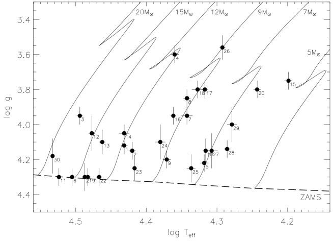
Our star sample covers a slightly broader temperature range than the standard definition for OB stars, with spectral types from B3 to O9. In the context of stellar evolution, the stars are located between the Zero Age (ZAMS) and the Terminal Age Main Sequence (TAMS). Their temperatures range from 16 000 to 34 000 K, the surface gravities from 3.6 to 4.3 in logarithmic scale, and the masses from 5 to 20 M⊙. The sample is listed in Table 1, where the spectral type, photometric quantities and atmospheric parameters derived in the Papers I-III are given. Object identifications include HD and HR numbers and names of the stars and our own numbering scheme to facilitate easy identification in the figures and other tables (i.e. stars analyzed in Paper I: #1-20, Paper II: #21-29, Paper III:#30).
For the whole sample, high-resolution échelle spectra at very high signal-to-noise () ratio – ranging from 250 up to over 800 in – and wide wavelength coverage were obtained, either by own observations, or from archives. Details on the observations and data reduction can be found in Papers I and III and for stars #21-29 in Simón-Díaz (2010). Spectra for stars #1–6 were obtained with Feros on the ESO 2.2m telescope in La Silla/Chile, with a resolving power of 48 000. Stars #7–16 were observed with Foces on the 2.2 m telescope at Calar Alto/Spain at a resolution of 40 000. Spectra of stars #17–20 were extracted from the archive of the Elodie échelle spectrograph mounted on the 1.93 m telescope of the Observatoire de Haute-Provence/France at 42 000. Spectra for stars #21-29 were obtained with Fies mounted at the 2.5 m Nordic Optical Telescope (NOT) in El Roque de los Muchachos observatory on La Palma (Canary Islands, Spain). A spectrum obtained with Feros for star #30 was extracted from the ESO Archive.
We aimed at selecting single stars, as second light from a companion of a similar spectral class distorts the ratio of line- to continuum-fluxes. Thus, objects in SB1 systems with much fainter companions (e.g. stars #21 and 26) can therefore still qualify as targets, because the contribution of the secondary star in optical light (UBV, uvby) is marginal. Individual components in a visual binary are also considered as targets (e.g. star #13 ). The star sample contains normal, Cephei and slowly pulsating B-stars111Pulsation periods of Cephei stars vary between 3 to 8 hours, while those in SPB stars vary between 0.5 to 3 days.. Exposures taken during a small fraction of the same night were co-added. The analysis will thus yield atmospheric parameters like effective temperature and surface gravity valid only for the moment of observation. For this sample, we have adopted reliable photometric data from the literature, these however correspond to a different moment of observation than for the spectroscopic data, which might be of significance for some variable stars.
3 Stellar parameter determination
Atmospheric parameters were determined simultaneously via line-fitting of synthetic spectra computed in NLTE to the observed data, as described in Papers I–III. Atmospheric parameters are the effective temperature , surface gravity , microturbulence , projected rotational velocity and macroturbulence . Details on the synthetic spectra and the quantitative analysis are summarized in the following.
3.1 Spectrum synthesis in NLTE
The analysis was based on a grid of synthetic spectra in NLTE computed with the codes Detail and Surface (Giddings 1981; Butler & Giddings 1985) on prescribed LTE atmospheric structures calculated with Atlas9 (Kurucz 1993b). Model atoms for H, He, C, N, O, Ne, Mg, Si and Fe for different ionization stages were employed. Opacities due to hydrogen and helium and the individual metals were considered in NLTE, and line blocking was accounted for in LTE via Kurucz’ Opacity Distribution Functions (Kurucz 1993a). This approach provides an efficient way to compute realistic synthetic spectra when the atmosphere is close to LTE. In particular, it is equivalent to full NLTE model atmosphere calculations for late O-type to early B-type stars with weak winds (Nieva & Przybilla 2007; Przybilla et al. 2011).
3.2 Quantitative spectral analysis
The spectral analysis follows the methodology introduced by Nieva (2007) and applied for H/He and C by Nieva & Przybilla (2007, 2008) and for other elements by Przybilla et al. (2008). Stellar parameters are determined through ionization equilibria for different species and Balmer lines fits. Spectroscopic indicators for effective temperature and surface gravity of the star sample are summarized in Table 4. Fitted spectra for stars #1,6,7 and 15 (Paper I) and #9 (Paper II), illustrate examples of global fits for different spectral classes. Numerous examples of fits to stellar spectral energy distributions (SEDs) can also be found in Papers I and III. The reliability of our temperature and gravity determinations and the minimisation of systematic uncertainties are confirmed by simultaneous agreement of several independent indicators: ionization equilibria of different atomic species, fits to Balmer lines and fits to the spectral energy distributions from the UV to the IR. Furthermore, our surface gravities are also confirmed by simultaneous match of ionization equilibria, fits to Balmer lines and the agreement of spectroscopic distances with Hipparcos distances (see Paper I). Note that every model atom for NLTE calculations is independent from each other, hence multiple ionization equilibria only render 4-5 independent indicators for temperature and gravity determinations.
The location of the (apparently slowly-rotating) sample stars in the - plane is visualized in Fig. 1, where also evolutionary tracks for non-rotating stellar models (Ekström et al. 2012) are shown for comparison. Both, the models and the stars have the same metallicity of = 0.014, the stars’ metallicities being determined in Papers I-III. The star sample provides us with a good coverage of the main-sequence band, ranging from 6 to 20 M⊙.
4 Temperature and gravity scales
Useful temperature scales for early-type stars have been presented by Napiwotzki et al. (1993), Daflon et al. (1999) and Lyubimkov et al. (2002), where the temperature can be estimated from reddening-independent photometric quantities (assuming a valid standard reddening-law). The first work scales the temperature to the 222-parameter from the narrow-band Strömgren -system. In contrast, the other two employ the 333-index from the broad-band Johnson -system. In all three cases, the temperature determination is based on other independent photometric calibrations or on fits to spectral energy distributions. Lyubimkov et al. (2002) proposed, in addition, temperature scales for two significantly different values of gravity.
Motivated by the aforementioned studies, we investigate whether new temperature and gravity scales to , , the Strömgren 444 and 555 is a measure of the stellar H line intensity can be established based on our previously derived spectroscopic parameters. Our atmospheric parameters derived simultaneously from several independent indicators and high quality spectral models and observations offer a unique set of input data for building such scales: uncertainties are as low as 1–2% for effective temperatures and 10% for surface gravities. This is in contrast to uncertainties of 5-10% and 25%, respectively, using standard methods. Typical uncertainties for effective temperature given in the literature are 3-5%, however these do not take into account the large discrepancies – up to 6000 K – that exist between different temperature determination methods. Error estimates of up to 40-60% in surface gravity are also found in the literature (see Sect. 5 for more details). Likewise, the most accurate photometric data available in the literature are adopted for this study. The compilation of photometric data is as homogeneous as possible, however for some objects, data are adopted from different sources. In addition, re-examinations of spectral types and luminosity classes were performed for the sample stars, as described in App. A. Stellar parameters, photometric indices, and their respective uncertainties, spectral types and luminosity classes adopted for the sample are listed in Table 1.
In the following, we present empirical relationships of atmospheric parameters and photometric indices based on data of our star sample. Note that the star sample does not cover uniformly the parameter space under consideration, therefore the relationships can be refined when adopting a more complete sample. Polynomial fits are chosen to directly compare our results to previous works from Napiwotzki et al. (1993), Daflon et al. (1999) and Lyubimkov et al. (2002). A few stars do not follow tightly the empirical fits for different reasons that need to be further investigated. Moreover, the correlation between effective temperature and surface gravity could be treated in an iterative manner in order to find an optimal solution, like the method proposed in Moon & Dworetsky (1984) and Napiwotzki et al. (1993). We aim at investigating this correlation with a larger sample of stars covering uniformely the parameter space in a further paper.
4.1 Spectroscopic parameters vs.
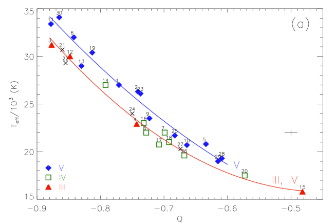
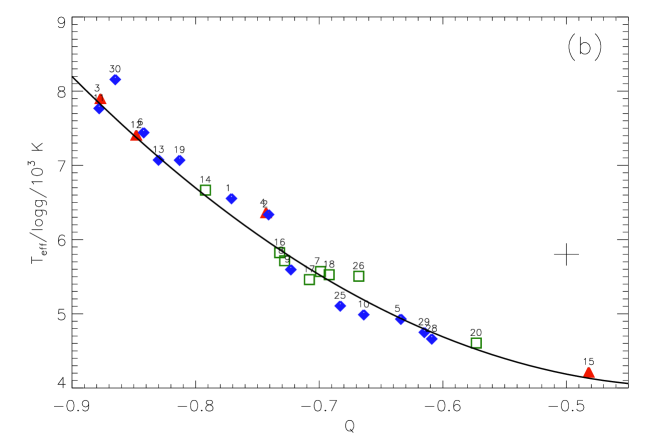
The reddening-free Johnson -index is particularly interesting for OB stars, as there are many distant objects in the Galactic spiral arms that at present do not have measurements in photometric systems other than the Johnson-system. Figure 2a shows the relation between our spectroscopic temperatures and , while Fig. 2b displays the behavior of vs. . The data from Table 1 are indicated by symbols and the polynomial fits by full lines, encoded for different luminosity classes as shown in the legend (in color in the online version). Four objects of luminosity class V had to be excluded from the analysis – marked with a cross in Fig. 2a (# 21, 22, 24 and 27). These stars are located in the Orion OB association. Stars # 21, 22 and 27 are located in a region of dense nebulosity and present anomalous reddening (see Table 1). In these cases, the -index should be re-evaluated using an appropriate reddening law, which is, however beyond the scope of the present paper.
The distinction of different luminosity classes reveals tighter trends of vs. than previously reported. The trends are consistent with those found by Nieva & Przybilla (2008) for a sub-set of stars (#1–6), where the parameter determination was based only on H, He and C. However, that sample was insufficient for a statistical analysis. In the present work, the polynomial fits for luminosity classes III and IV converge into a single curve and the scale for luminosity class V is 1500 to 2000 K hotter. The minimisation of uncertainties in our parameter determination and the high accuracy of the photometric data allow clear trends for different luminosity classes to be distinguished. In contrast, standard parameter determinations may provide larger systematic uncertainties (see Sect. 5), that would prevent the relations found here to be identified.
The relationship between the temperature and for different luminosity classes, i.e., different evolutionary stages, displayed in Fig. 2a can be expected by the fact that stars closer to the ZAMS are more compact and bluer, therefore hotter than the more evolved giants at similar masses.
In contrast, the ratio vs. does not show a dependence on the luminosity class (Fig. 2b), since all three polynomial fits converge approximately to a single solution. Therefore, we adopt one fit to the whole sample (except for the excluded stars), indicated by the thick black curve.
Temperature and gravity scales to the Johnson -parameter are proposed, based on the curves displayed in Figs. 2a,b. Polynomial fits result in the following equations for the different luminosity classes:
| (1) |
| (2) |
| (3) |
The range where these equations are valid are delimited by the observational data, as indicated in Figs. 2a,b. Note that the parameter range of interest is not uniformly sampled by the observations (Fig. 1), a further addition of few hotter stars with lower surface gravities will allow to refine the fits from the present work. The internal and external uncertainties of and are listed in Table 2. The internal uncertainty measures the 1-dispersion of the residuals of the fitted values and the spectroscopic parameters and it depends on the quality of the polynomial fits. The external uncertainty is calculated via error propagation of the parameters involved and it depends on the uncertainties of the spectroscopic and photometric parameters, and on the reliability of luminosity classifications. Luminosity classes are the largest sources of external errors , as the relationship between temperature and the -index for luminosity class V is up to 2000 K hotter than that for III,IV. The precision of the parameter determination is as indicated in Table 2 only when accurate photometric data and a reliable luminosity class is given for the star666Luminosity classes from Simbad from different sources might differ from each other. See Nieva & Przybilla (2008) and Firnstein & Przybilla (2012) for corrections of luminosity classes of the Simbad database..
When the luminosity class is not known or is not reliable, the uncertainty in the derived temperature increases to 1500 K, which is still smaller than the differences between various temperature determinations in the literature (they can amount up to 2000 K and in extreme cases up to 6000 K; see Sect. 5 for more details). In the case of the gravity, the lack of precise luminosity classes causes an error of 0.2 dex, that is also smaller than the maximum differences shown in the literature of 0.4 dex. Uncertainties in temperature of 1500 K and in gravity of 0.2 dex are, however, too large for some further applications, such as precise chemical abundance determinations or precise derivation of mass, radius and distances of stars. Despite the luminosity classification can compromise the accuracy of temperature and gravity, our calibrations are a useful tool to estimate such parameters for further applications. Therefore, and can be employed as starting points to be refined using, e.g. spectroscopic analyses.
4.2 Spectroscopic parameters vs.
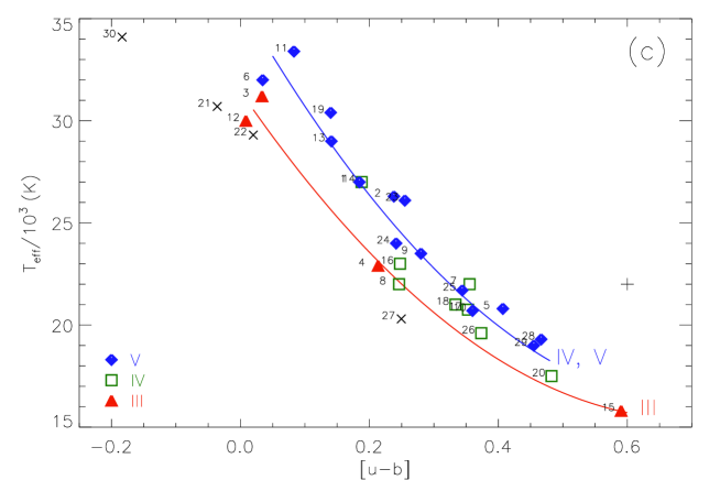
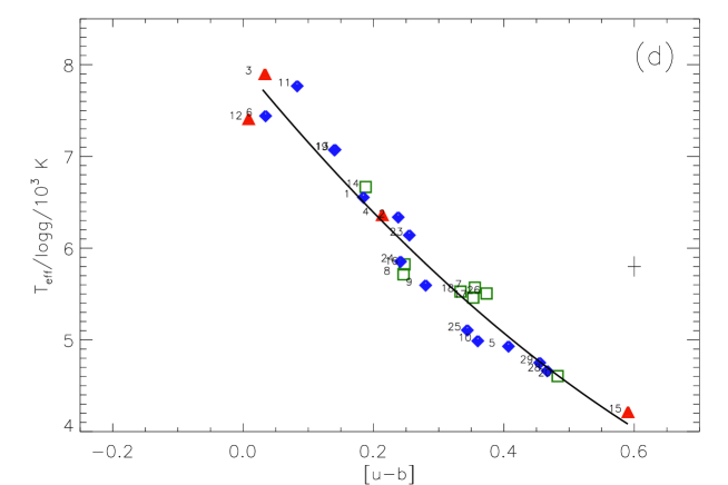
In this section we investigate a scale based on the narrow-band Strömgren colors for estimating effective temperatures and gravities. Figures 2c,d show the relationship between and our spectroscopic temperatures and , respectively. The data are encoded like in Figs. 2a,b. Four objects had to be excluded from the analysis – marked with a cross in Fig. 2c. Stars # 21, 22 and 27 have anomalous reddening and star #30 is apparently too hot for the relationship found for the rest of the main sequence stars777Napiwotzki et al. (1993) propose an upper limit of 30 000 K for this relationship.. Similarly to the case of the -parameter, trends of vs. are found for different luminosity classes. In this case, the polynomial fits for luminosity classes IV and V converge into a single relation, while the scale for luminosity class III is 2000 to 4000 K cooler. In addition, vs. does also not indicate a dependence on the luminosity class (Fig. 2d). The curves displayed in Figs. 2c,d are employed to propose a temperature and gravity scale to the Strömgren photometric parameter . Polynomial fits to the data result in the following equations for the different luminosity classes:
| (4) |
| (5) |
| (6) |
Similarly to the case of the -parameter, the range where these equations are valid are determined by the observational data. The internal and external uncertainties of and are listed in Table 2. When the luminosity class is not known or not precise, the error in the derived temperature increases to 2000 K and for gravity to dex, both larger than in the case of the calibrations to .
4.3 Spectroscopic parameters vs. and
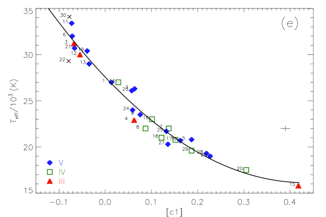
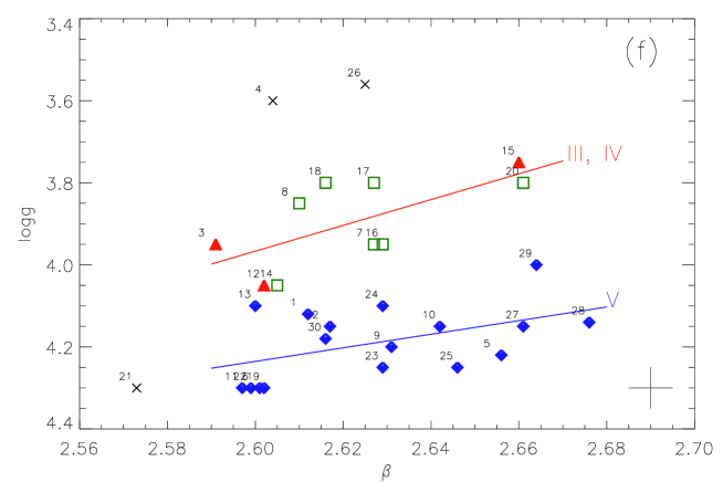
The Strömgren parameters and have been defined as tools to estimate and in early-type stars. A single trend for the effective temperature vs. (Fig. 2e) and two curves for vs. (Fig. 2f) are found. For the latter, the relationship for luminosity class V is 0.3 dex higher than for III/IV. Stars #4 and 26 have been excluded from the fits because their gravities are too low in comparison with the rest of the stars of luminosity class III/IV (they lie slightly above the TAMS in Fig. 1). Star # 21 is also excluded, as there is a large nebular emission feature centered on H, that causes a significantly reduced value of the -index. As the parameter range of interest is not uniformly sampled by the observations (Fig. 1), a further addition of few hotter stars with low surface gravities and/or cooler stars on the ZAMS might produce a flattening of the slope for luminosity class V in Fig. 2f, which remains to be investigated.
Polynomial fits to the present data result in the following equations:
| (7) |
| (8) |
| (9) |
The uncertainties are listed in Table 2. If the luminosity class is not well known, the error in the surface gravity determination increases to 0.25 dex.
4.4 Spectroscopic parameters vs. fitted values
| Int. | Ext. | Int. | Ext. | |||
|---|---|---|---|---|---|---|
| V | : | 738 K | 800 K | : | 0.08 | 0.23 |
| III,IV | : | 385 K | 530 K | : | 0.08 | 0.17 |
| IV,V | : | 1060 K | 300 K | : | 0.19 | 0.02 |
| III | : | 960 K | 280 K | : | 0.19 | 0.04 |
| V | : | 1060 K | 290 K | : | 0.07 | 0.01 |
| III,IV | : | 1060 K | 290 K | : | 0.08 | 0.01 |
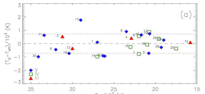
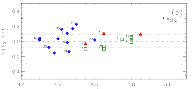
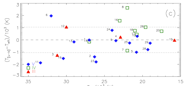
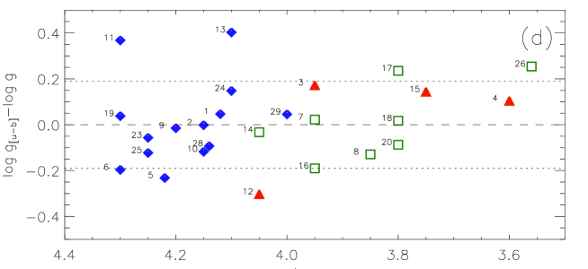
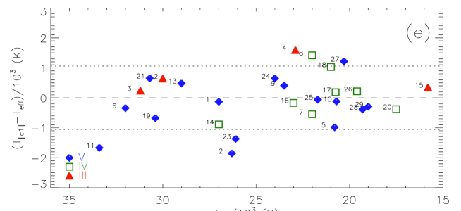
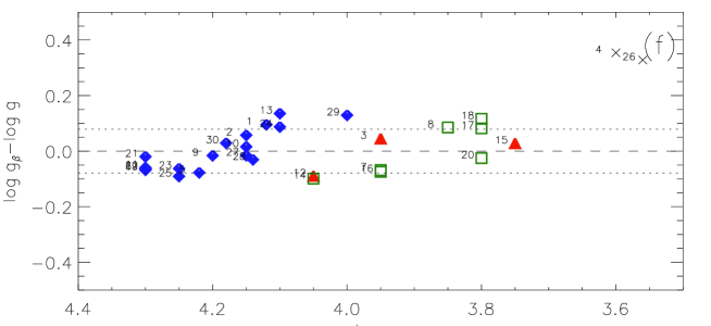
Internal uncertainties of our calibrations are analysed here via residuals of the fitted values to the spectroscopic parameters, as displayed in Fig. 3. In the left panels (a), (c) and (e) are compared to and in the right panels (b), (d) and (f) are compared to . Dotted lines indicate internal uncertainties like in Table 2 for calibrations independent of the luminosity class (= 0.08 dex, = 0.19 dex and = 1060 K). Otherwise, they indicate averaged 1 values for different luminosity classes weighted by star number (= 700 K, = 1040 K and = 0.08 dex). Dashed lines indicate perfect agreement and symbols are encoded as in the legend. Stars #4 and 26 were excluded from the fits in Fig. 3f as they are too evolved (i.e., beyond core H-burning) in comparison to the rest of the sample.
As indicated in Table 2, the internal uncertainties based on are smaller than in the other cases, but the external uncertainties are larger. In further comparisons to other work, we take as reference values the internal uncertainties based on : for temperature = 700 K (averaged value for different luminosity classes weighted by star number) and for gravity = 0.08 dex, as in Fig. 3. This is because our special interest in the -based calibrations, as there are more stars with measured UVB indices than with other filters.
5 Our spectroscopic parameters vs. other works
5.1 Photometric calibrations
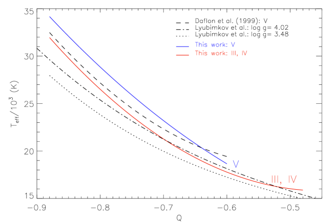
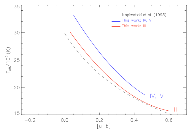
Our -scales derived from multiple ionization equilibria are compared in Fig. 4a to photometric calibrations of Daflon et al. (1999) for luminosity class V and of Lyubimkov et al. (2002) for 3.48 and 4.02. In addition, our -scales are compared to that of Napiwotzki et al. (1993) in Fig. 4b. Our scales tend to be hotter at higher temperatures than the photometric scales.
Our for luminosity class V (upper solid curve, blue in the online version) is 2000 K hotter than that proposed by Daflon et al. (1999) at the highest temperature, the difference decreasing until both scales cross each other at 21 000 K, and remain similar at slightly lower . The comparison to Lyubimkov et al. (2002) has to be done more cautiously because our sample has a variety of surface gravity values. Only four stars have similar gravities to 4.00: #3 (III), 7 (IV), 16 (IV) and 29 (V). We compare their upper curve (dashed dotted line) to our lower curve (solid line, red in the online version). Our relation is 2000 K hotter than theirs at the highest temperatures and both practically coincide below 21 000 K.
Figure 4b shows the comparison of our to the calibration proposed by Napiwotzki et al. (1993) in their Eqn. 9. Their and our curve for luminosity class III practically coincide below 19 000 K, and the smallest discrepancy to our IV,V relation is 1500 K at 18 000 K. In contrast, our scales are steeper than their curve, resulting in larger differences at higher , with maximum values of 1500 K for luminosity class III and 6000 K for IV,V. Possible reasons for these discrepancies are discussed at the end of next section.
5.2 Other determinations for individual stars
Besides the photometric temperature scales discussed in Sect. 5.1, other determinations of temperature and surface gravity are found in the literature for several stars of the sample. Whenever possible, we also compare values of microturbulence as all parameters are interrelated. Figures 5-9 illustrate the differences between the atmospheric parameters derived in other works and our spectroscopic (a), (b) and (c). Dashed lines indicate full agreement between other determinations and our values, and dotted lines in Figs. 5-9a,b denote (700 K) and (0.08 dex), like in Fig. 3, as a reference to our photometric scale. Note that uncertainties in our spectroscopic parameters are even smaller than the -errors for the -calibrations: 300 K for and 0.05 dex for .
It is beyond the scope of this paper a detailed description of other analysis methods and the causes of discrepancies between their and our results. Based on our previous studies (Nieva & Przybilla 2007, 2008, 2010a, 2010b), we propose possible reasons that might cause systematic offsets. However, we should bear in mind that in most cases the discrepancies are likely due to a combination of various effects, which are difficult to be quantified beforehand.
Kilian et al. (1991).
This work presents a spectroscopic determination of gravity and effective temperature of stars in the solar neighborhood from NLTE hydrogen line profiles (H, H, H) and the silicon ionization equilibria Si ii/iii and/or Si iii/iv (depending on the stellar temperature). Their procedure is similar to ours, based on an earlier version of the codes Detail and Surface, however with fewer spectroscopic indicators than those shown in Table 4. Their silicon abundances are based on the model atom by Becker & Butler (1990)888We do not analyse Si ii lines because their synthetic spectrum provides erroneous line intensities, as reported in Simón-Díaz (2010) and Nieva & Simón-Díaz (2011)., like in our case, but on model atmospheres by Gold (1984) with much less line blanketing than ATLAS9. Their microturbulences are derived in the standard way from O ii lines. Figure 5 displays comparisons between their and our stellar parameters for 11 stars in common, identified like in Table 1. A clear trend is noticed in Fig. 5a for effective temperatures, being their values 2000 K higher at 20 000 K and 2000 K lower at 34 000 K. Less blanketed model atmospheres affect the line-blocking and hence the temperature structure of the stellar atmosphere.This could be a reason for discrepancies with our temperatures. Furthermore, for cooler stars, the use of Si ii in the ionization equilibrium can also cause an offset in the derived temperature. In contrast, their gravities agree with our spectroscopic values and lie within the 1 uncertainty of for most stars (Fig. 5b). Their microturbulences tend to be larger than ours (Fig. 5c), reaching a maximum difference of 6 km s-1.
Cunha & Lambert (1992).
The parameters determined in this work were used in a series of subsequent studies of stars in the Orion region by Cunha & Lambert (1994), Cunha et al. (2006), Lanz et al. (2008), and Daflon et al. (2009). Their approach for deriving effective temperatures and surface gravities is based on an iterative scheme using older calibrations of Strömgren photometry modified by Gies & Lambert (1992) coupled with fits to the wings of H profiles computed in LTE (Kurucz 1979). Microturbulences were determined from O ii lines in NLTE. Figure 6 displays the differences between their and our parameters for 13 stars in common. In spite this sample differs from that in the comparison with Kilian et al. (1991), we notice in Fig. 6a an overall similar trend in temperature than in Fig 5a, except for star #22. But in this case, there are more stars with temperatures within our 1 uncertainty margins for . It is difficult to identify the sources of discrepancies in temperature. They could be related to the details of the photometric calibrations, i.e. the use of less blanketed model atmospheres to compute the synthetic photometric indices and to the fits to H in LTE in the iterative procedure. Concerning the gravities (Fig. 6b), their values are higher (up to 0.4 dex) than our spectroscopic gravities for most stars, lying above the 1 uncertainty of our calibration. An exception is the star #21, that shows a difference of 0.4 dex to our value. The discrepancies in surface gravities could be related to the use of LTE synthetic profiles of H, that have been shown to give larger gravities than those computed in NLTE (Nieva & Przybilla 2007). Since their approach is iterative, this also would affect the determination of temperature. However, differences larger than 0.2 dex cannot be explained with NLTE effects on the Balmer lines wings. The continuum normalization of H could also play a role in this respect, since this is an important source of uncertainty in surface gravity determinations (Nieva & Przybilla 2010a, b). Their microturbulences are larger – by 5 to 10 km s-1 – than those derived by us.
In contrast, in Cunha et al. (2006), Lanz et al. (2008) and Daflon et al. (2009)999Parameters for 2 stars in common have been revised in Daflon et al. (2009) via S ii/iii ionization equilibrium. For star #1, offsets of 530 K and 0.05 dex and for #24, 480 K and 0.05 dex in temperature and surface gravity, respectively, have been applied. the stars # 11, 21, 22, 27 and 28 were excluded from the studies, which lead to maximum differences to our work in of up to 1000 K and in of 0.05-0.3 dex. I.e., the selected sub-sample of stars analyzed in those works presents a better agreement with our results than the original complete sample from Cunha & Lambert (1992), however a systematic offset in gravities and microturbulences still persists.


Morel & Butler (2008).
This work presents an interesting comparison between atmospheric parameters derived in a standard iterative spectroscopic way, i.e. via NLTE Si ii/iii and/or Si iii/iv ionization equilibria (Morel et al. 2006) and an new Ne i/ii ionization equilibrium. In addition, the fits of NLTE profiles to H, H, H and H are used for surface gravity determination. The computations are performed with similar versions of Detail and Surface and the same model atmospheres than those used by us. For Si, a model atom by D. J. Lennon is employed (Trundle & Lennon 2005) while for Ne a new model by K. Butler is applied for the first time. Temperatures derived with Ne are cooler by 825 K than those derived with Si. In both cases, microturbulences were determined from O ii lines. It is worth noticing that they have analyzed 3 stars that were excluded from our first sample (Paper I) because they turned out to be double-lined spectroscopic binaries, namely HD 35468 (HR 1790, Bellatrix), HD 163472 (HR 6684, V2052 Oph) and HD 214993 (HR 8640, 12 Lac). Our samples share 6 stars, which parameters are compared in Fig. 7. Overall, we notice a trend in temperature (Fig. 7a) in a similar way then the two previous cases, the maximum differences being 1000 at 21 000 K and 2000 K at 27 000 K.
It is difficult to evaluate the causes of discrepancies in the results. It is not clear whether the new Si ii model atom provides improved line intensities than the model by Becker & Butler (1990). If the problem persists, it would affect temperatures lower than 23 000 K (the exact limit depends on the S/N of the spectrum). In addition, the Ne model applied in Morel & Butler (2008) showed difficulties to achieve Ne i/ii ionization equilibrium and to match the temperatures derived with Si ii/iii/iv ionization equilibria. This Ne model atom was subsequently improved with more accurate values in Przybilla et al. (2008) resulting in consistent results between Ne i/ii and other ionization equilibria: He i/ii, C ii/iii/iv, O i/ii, Si iii/iv, removing discrepancies found previously; see also Table 4 of the present paper. Furthermore, their surface gravities (Fig. 7b) are 0.1-0.45 dex lower than those found by us. These offsets are unexpected, as their analysis is based on the same codes and a similar H model than those employed in our work. An offset in the temperature determination is not sufficient to explain such large differences in . The remaining sources of systematics to be investigated in those results is the continuum normalization of the Balmer lines (Nieva & Przybilla 2010a, b), that might cause differences larger than 0.2 dex in the derived surface gravities. Finally, there is a hint of a trend in microturbulences, except for star #6 (Fig. 7c).
Simón-Díaz (2010).
Stellar parameters were determined in this work spectroscopically by fitting the Balmer lines and matching He i/ii and/or Si iii/iv ionization equilibria. The spectrum synthesis was computed with the unified atmosphere code Fastwind (Puls et al. 2005), that models the stellar atmosphere and wind simultaneously in NLTE. The same observed spectra than those analyzed in Paper II have been analyzed in Simón-Díaz (2010). Despite the different atmospheric structure, input atomic data and line-formation computations, the temperatures and gravities derived in this work agree overall very well with our determinations, as can be seen from Figs. 8a,b, i.e., the differences lie within the 1-uncertainty of the -calibrations for most stars. Microturbulences also show a good agreement, considering the different computations, reaching a maximum difference of 4 km s-1 (Fig. 8c).
Napiwotzki et al. (1993).
In Sect. 5, our calibrations were compared with that proposed by Napiwotzki et al. (1993). In Fig. 9a,b, our spectroscopic parameters are compared to temperatures and gravities computed with an improved version by Napiwotzki et al. (1993) of a code by Moon & Dworetsky (1984). Fig. 9c shows a comparison of our spectroscopic temperatures to those derived with the -temperature scale by Napiwotzki et al. (1993). The code uses as input Strömgren indices and interpolates within a grid of synthetic colors iteratively until convergence in effective temperature and surface gravity is reached. The modification by Napiwotzki et al. (1993) on the gravities is based on fits to Balmer lines. The code provides a final temperature and gravity, hereafter TN93 and , respectively. It also returns a temperature from their calibration to the -parameter, hereafter , that corresponds to their Eqn. 9, discussed in Sect. 5.1 (see also Fig. 4b).
Figure 9a displays the difference between their and our . There is a very good agreement for lower temperatures, up to = 24 000 K. At higher temperatures there is a larger scatter, their values being smaller than ours from a few hundred up to 3000 K. Exceptions are star #12, with perfect agreement, and star #22, 2500 K hotter in their approach. We recall that a non-standard reddening law is found for this star, as it is located in a dense nebulous region, therefore a photometric determination of its parameters is dubious. The vertical dashed-dotted line in Fig. 9a corresponds to the upper temperature limit to which they expect their determination to be valid. Thick squares denote stars with 30 000 K and diamonds the rest of the sample; this corresponds to the upper limit to which they expect their method to be valid. From Fig. 9a we notice, however, that their upper limit is likely 24 000 K. Figure 9b shows the differences between their gravities, , and our . There is a good agreement between both methods for several stars. A few objects also show larger discrepancies up to 0.3 dex for stars denoted with diamonds and, as expected, even larger for those marked with squares, with temperatures beyond their upper limit (0.6 dex for star #30 and 0.5 dex for star #21, not shown in Fig. 9b because they lie outside the plot range). Their , extracted from the same code, is compared with our spectroscopic temperature in Fig. 9c. The differences to our work show a similar behaviour than Fig. 9a, but with a larger scatter. Stars #2, 21 and 30 are not shown because their differences are larger than 3000 K. Following the comparisons in Fig. 9, we recommend to adopt for 24 000 K when using their approach.
Several reasons could lead to discrepancies between their and our results at higher temperatures. We note that only four stars hotter than 24 000 K are present in their calibration sample to derive the -scale. Three of these stars have luminosity class III, therefore the -scale underestimates temperature of stars with luminosity class V (most objects in this work). Two of these four stars are present in our sample: #3 and #19. for star #3 (HD 63922, HR 3055) is 1200 K lower than our value, and that for star #19 (HD 34816, HR 1756) is 2800 K than our temperature. Furthermore, their calibration is based on temperatures from Malagnini et al. (1986), determined from comparisons of observed spectral energy distributions to fluxes computed in LTE by Kurucz (1979). Hence, discrepancies with our results could also be caused by less line blanketing in their model atmospheres, neglection of NLTE effects in the fluxes, and also in the computation of synthetic indices and Balmer lines.
| Sp. T | # | |||||||
| O9 V | 30 | 34100 | 4.18 | 3.23 | 33000 | 3.33 | … | 34 000 |
| B0 V | 11 | 33400 | 4.30 | 3.15 | 30000 | 3.16 | … | 30 000 |
| B0.2 V | 6 | 32000 | 4.30 | 3.05 | … | … | … | … |
| B0.5 V | 21 | 30700 | 4.30 | 2.98 | … | … | … | … |
| 19 | 30400 | 4.30 | 2.95 | |||||
| 22 | 29300 | 4.30 | 2.88 | |||||
| B0.7 V | 13 | 29000 | 4.10 | 2.83 | … | … | … | … |
| B1 V | 1 | 27000 | 4.12 | 2.65 | 25400 | 2.70 | 24620 | … |
| 2 | 26300 | 4.15 | 2.59 | |||||
| B1.5 V | 23 | 26100 | 4.25 | 2.63 | … | … | … | … |
| 24 | 24000 | 4.10 | 2.43 | |||||
| 9 | 23500 | 4.20 | 2.38 | |||||
| B2 V | 25 | 21700 | 4.25 | 2.19 | 22000 | 2.35 | 19500 | 20900 |
| 5 | 20800 | 4.22 | 2.06 | |||||
| 10 | 20700 | 4.15 | 2.06 | |||||
| 27 | 20300 | 4.15 | 2.02 | |||||
| B2.5 V | 28 | 19300 | 4.14 | 1.90 | 18700 | 1.94 | 16000 | … |
| 29 | 19000 | 4.00 | 1.85 | |||||
| B1 IV | 14 | 27000 | 4.05 | 2.67 | … | … | … | … |
| B1.5 IV | 16 | 23000 | 3.95 | 2.32 | … | … | … | … |
| 8 | 22000 | 3.85 | 2.18 | |||||
| B2 IV | 7 | 22000 | 3.95 | 2.20 | … | … | … | … |
| 18 | 21250 | 3.80 | 2.11 | |||||
| 17 | 20750 | 3.80 | 2.05 | |||||
| B3 IV | 20 | 17500 | 3.80 | 1.65 | … | … | … | … |
| 18 | 21250 | 3.80 | 2.11 | |||||
| B0.2 III | 3 | 31200 | 3.95 | 2.92 | 29000 | 2.88 | … | … |
| B0.5 III | 12 | 30000 | 4.05 | 2.88 | … | … | … | … |
| B3 III | 15 | 15800 | 3.75 | 1.38 | 17100 | 1.60 | … | … |
5.3 Our recommended parameter determination
Our scales derived spectroscopically tend to be hotter at higher temperatures than the photometric scales proposed by Daflon et al. (1999), Lyubimkov et al. (2002) and Napiwotzki et al. (1993). Furthermore, our values also tend to be higher at 25 000 K and lower at lower temperatures when compared with values derived by Kilian et al. (1991), Cunha & Lambert (1992) and Morel & Butler (2008) using different analysis methods, synthetic spectra and observations. In contrast, we note that temperatures determined by Simón-Díaz (2010) using the same set of high-quality spectra than those analysed by us, other state-of-the-art model atmosphere and spectral synthesis in NLTE and simultaneous silicon ionization equilibria and fits to Balmer and helium lines, render values in agreement to our determinations. The excellent agreement between our and Simón-Díaz (2010) temperatures lead us to conclude that our temperature determination based on high quality data, state-of-the-art spectral synthesis in NLTE and several independent temperature indicators are reliable and almost free of large remaining systematic effects. If adopting significantly different values in the higher temperature domain, like suggested by previous studies, the ionization equilibrium of no species will be matched any longer, hence the global and detailed observed spectra will not be reproduced by the synthetic model.
We recommend, when possible, to perform a parameter determination like the full spectroscopic method presented by us in previous works (e.g. Paper I) or by Simón-Díaz (2010). If the observed spectra or the spectral synthesis are not available, a good parameter estimation can be provided by our scales presented in Sect. 4 of this work. For 24 000 K, the scale by Napiwotzki et al. (1993) also renders reliable temperatures, and for 21 000 K, the scales by Daflon et al. (1999) and Lyubimkov et al. (2002) also give reliable results (note the lower limit indicated by each scale).

6 Spectral type calibration
In App. A, we re-evaluate the spectral classification of the sample stars. Slight revision of spectral sub-types and luminosity classes have been performed in several stars, as indicated in Table 1. The relationship between spectral types and luminosity classes and the stellar parameters , as well as their corresponding value of bolometric correction () is summarized in Table 3. There, also recommended values of temperature and/or from Schmidt-Kaler (1982), Gray & Corbally (1994) and Cox (2000) are given for comparison.
In cases where more than one star belong to a certain spectral/luminosity class, instead of adopting an average value for the parameters, we prefer to indicate the exact parameters of the stars to see how much can they variate. Stars #4 and 26 have been excluded from the calibration because they seem to be too evolved in comparison to the rest of the objects, as explained above. Our star sample is not large enough to cover all possible combinations of spectral and luminosity classes within the range O9-B3 V-III, however the carefully derived data allow us to anchor a spectral type calibration to empirical values of temperature for luminosity class V and partially also for luminosity classes III and IV. Our calibration tends to be hotter than previous reference values in most cases. This is in accordance with our photometric temperature calibrations, that are in general hotter than previous work. This table is also very useful to estimate stellar parameters once the spectral and luminosity classification are well known.
7 Bolometric corrections vs. temperature
Bolometric corrections play an important role in the determination of luminosities and indirectly also of other fundamental stellar parameters computed from atmospheric parameters and , e.g. radii, masses. Fundamental parameters can be directly compared to predictions from evolution models in order to learn more about the physics of the stars.
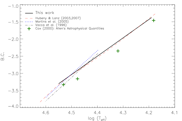
Taking advantage of our accurate atmospheric parameters determined spectroscopically for the present sample, we derive a semiempiric relationship for as a function of . Bolometric corrections are computed from spectral fluxes calculated with Atlas9101010Atmospheric structures and fluxes of OB main sequence and giant stars computed in LTE are equivalent to the full NLTE approach. See Nieva & Przybilla (2007) and Przybilla et al. (2011) for details. for each star of the sample using their corresponding values of and . As expected, a clear relationship is found for vs. (Fig. 10, left panel), practically independent from the luminosity class or the surface gravity. Figure 10, right panel, illustrates a comparison of our relationship to other work by Vacca et al. (1996), Cox (2000), Hubeny & Lanz (2003, 2007), and Martins et al. (2005) derived mainly from synthetic models. Our slope is less steep than those by Vacca et al. (1996) and Martins et al. (2005), our calibration extending to lower temperatures. In addition, our fit agrees with from Hubeny & Lanz (2003, 2007) and for temperatures higher than 32 000 K also with those by Martins et al. (2005). In contrast, reference values for recommended by Cox (2000) are systematically lower than our data.
From the relationship found in Fig. 10 (left panel), we propose a new calibration of the bolometric correction as a function of :
| (10) |
8 Summary and conclusions
Based on comprehensive previous studies which lead us to determine effective temperatures and surface gravities of 30 OB-type (O9-B3 V-III) stars at high accuracy and precision, here we investigate whether such parameters can be used to propose new calibrations to some photometric indices. The spectroscopic parameters were derived via multiple ionization equilibria and simultaneous fits to the Balmer lines based on our most recent spectrum synthesis for NLTE computations and high-quality observed spectra. We propose very useful relationships between atmospheric parameters and various photometric indices from the Johnson and the Strömgren systems. Effective temperatures can be estimated at a precision of 400 K for luminosity classes III/IV and 800 K for luminosity class V. And surface gravities can reach internal uncertainties as low as 0.08 dex when using our calibration to the Johnson -parameter. Similar precision is achieved for gravities derived from the -index and the precision decreases for both atmospheric parameters when using the Strömgren indices and . In contrast, external uncertainties are larger for the Johnson than for the Strömgren calibrations. Our uncertainties are smaller than typical differences among other methods in the literature, reaching values up to 2000 K for temperature and 0.25 dex for gravity, and in extreme cases, 6000 K and 0.4 dex, respectively. We had further re-examined the luminosity and the spectral classes for the star sample and also propose a parameter calibration for sub-spectral types. Furthermore, we present a new bolometric correction relation to temperature based on our empirical data, rather than on synthetic grids.
The photometric calibrations presented here are useful tools to estimate effective temperatures and surface gravities of non-supergiant OB stars in a fast manner. Caution has to be taken for undetected double-lined spectroscopic binaries and single objects with anomalous reddening-law, dubious photometric quantities and/or luminosity classes, for which the external uncertainties may increase significantly. We recommend to use these calibrations only as a first step for parameter estimation, with subsequent refinements based on spectroscopy.
Acknowledgements.
The author acknowledges a FFL stipend from the University of Erlangen-Nuremberg and thanks Norbert Przybilla, Eva Ziegerer, Christian Heuser, Ulrich Heber and Sergio Simón-Díaz for their suggestions, and the anonymous referee for his/her comments leading to substantial improvements of the paper.References
- Anders & Grevesse (1989) Anders, E., Grevesse, N. 1989, Geoch. et Cosmoch. Acta, 53, 197
- Becker & Butler (1990) Becker, S. R., & Butler, K. 1990, A&A, 235, 326
- Butler & Giddings (1985) Butler, K., & Giddings, J. R. 1985, in Newsletter of Analysis of Astronomical Spectra, No. 9 (Univ. London)
- Briquet et al. (2011) Briquet, M., Aerts, C., Baglin, A., et al. 2011, A&A, 527, 112 (Paper III)
- Cantiello et al. (2009) Cantiello, M., Langer N., Brott, I. et al. 2009, A&A, 499, 279
- Cunha et al. (2006) Cunha, K., Hubeny, I. & Lanz, T. 2006, ApJ, 647, 143
- Cunha & Lambert (1992) Cunha, K., & Lambert, D. L. 1992, ApJ, 399, 586 (CL92)
- Cunha & Lambert (1994) Cunha, K., & Lambert, D. L. 1994, ApJ, 426, 170
- Cox (2000) Cox, A. 2000, Allen’s Astrophysical Quantities (Springer, New York)
- Daflon et al. (1999) Daflon, S., Cunha, K. & Becker, S.R. 1999, ApJ, 522, 950
- Daflon et al. (2009) Daflon, S., Cunha, K., de la Reza, R. et al. 2009, ApJ, 138, 1577
- Ekström et al. (2012) Ekström, S., Georgy, C., Eggenberger, P. et al. 2012, A&A, 537, 146
- Firnstein & Przybilla (2012) Firnstein, M., & Przybilla, N. , A&A, in press
- Conti & Alschuler (1971) Conti, P. S., & Alschuler, W. R. 1971, ApJ, 170, 325
- Giddings (1981) Giddings, J. R. 1981, Ph.D. Thesis, London
- Gies & Lambert (1992) Gies, D. R., & Lambert, D. L. 1992, ApJ, 339, 586
- Gold (1984) Gold, M. 1984, Diploma Thesis, Munich
- Grevesse & Sauval (1998) Grevesse, N., & Sauval, A. J. 1998, Space Sci. Rev., 85, 161
- Gray & Corbally (1994) Gray, R. O., & Corbally, C. J. 1994, AJ, 107, 742 (GC94)
- Gray & Corbally (2009) Gray, R. O., & Corbally, C. J. 2009, Stellar Spectral Classification (Princeton University Press, Princeton)
- Hauck & Mermilliod (1998) Hauck, B., & Mermilliod, M. 1998, A&AS, 129, 431
- Hoffleit & Jaschek (1982) Hoffleit, D., & Jaschek, C. 1982, The Bright Star Catalogue, 4th ed. (Yale University Observatory, New Haven)
- Hubeny & Lanz (2003) Hubeny, I., & Lanz, T. 2003, ApJS, 146, 417
- Hubeny & Lanz (2007) Hubeny, I., & Lanz, T. 2007, ApJS, 169, 83
- Jaschek & Jascheck (1987) Jascheck, C. & Jascheck, M. 1987, The classification of stars (Cambridge University Press, Cambridge)
- Kilian et al. (1991) Kilian, J., Becker, S. R., Gehren, T. & Nissen, P. E. 1991, A&A, 244, 419
- Kurucz (1979) Kurucz, R. L. 1979, ApJS, 40, 1
- Kurucz (1993a) Kurucz, R. L. 1993a, CD-ROM No. 2–12 (SAO, Cambridge, Mass.)
- Kurucz (1993b) Kurucz, R. L. 1993b, CD-ROM No. 13 (SAO, Cambridge, Mass.)
- Lanz et al. (2008) Lanz, T., Cunha, K., Holtzman, J. & Hubeny, I. 2008, ApJ, 678, 1342
- Lyubimkov et al. (2002) Lyubimkov, L.S., Rachkovskaya, T.M., Rostopchin, S.I. & Lambert D.L. 2002, MNRAS, 333, 9
- Malagnini et al. (1986) Malagnini, M. L., Morosi, C., Rossi, L. & Kurucz, R. L. 1986, A&A, 162, 140
- Martins et al. (2005) Martins, F., Schaerer, D. & Hillier, D. J. 2005, A&A, 436, 1049
- Mermilliod (1991) Mermilliod, J. C. 1991, Catalogue of Homogeneous Means in the UBV System (Institut d’Astronomie, Université de Lausanne)
- Meynet & Maeder (2003) Meynet, G., & Maeder, A. 2003, A&A, 411, 543
- Moon & Dworetsky (1984) Moon, T. T., & Dworetsky, M. M. 1984, Observatory, 104, 273
- Morel & Magnenat (1978) Morel, M., & Magnenat, P. 1978, A&AS, 34, 477
- Morel et al. (2006) Morel, T., Butler, K., Aerts, C. & Briquet, M. 2006, A&A, 457, 651
- Morel & Butler (2008) Morel, T., & Butler, K. 2008, A&A, 487, 307 (MB08)
- Napiwotzki et al. (1993) Napiwotzki, R., Schönberner, D. & Wenske, V. 1993, A&A, 268, 653
- Nieva (2007) Nieva, M. F. 2007, Ph.D. Thesis, Erlangen-Nuremberg and Observatório Nacional, Brazil
- Nieva & Przybilla (2007) Nieva, M. F., & Przybilla, N. 2007, A&A, 467, 295
- Nieva & Przybilla (2008) Nieva, M. F., & Przybilla, N. 2008, A&A, 481, 199
- Nieva & Przybilla (2010a) Nieva, M. F., & Przybilla, N. 2010a, in ASP Conf. Ser., 425, 146
- Nieva & Przybilla (2010b) Nieva, M. F., & Przybilla, N. 2010b, EAS Publ. Ser., 43, 167
- Nieva & Przybilla (2012) Nieva, M. F., & Przybilla, N. 2012, A&A, 539, A143 (Paper I)
- Nieva & Simón-Díaz (2011) Nieva, M. F., & Simón-Díaz 2011, A&A, 532, 2 (Paper II)
- Przybilla et al. (2008) Przybilla, N., Nieva, M. F., & Butler, K. 2008, ApJ, 688, L103
- Przybilla et al. (2011) Przybilla, N., Nieva, M. F., & Butler, K. 2011, JPhCS, 328, 012015
- Puls et al. (2005) Puls, J., Urbaneja, M., Venero, R. et al. 2005, A&A, 435, 669
- Schaller et al. (1992) Schaller, G., Schaerer, D., Meynet, G., & Maeder, A. 1992, A&AS, 96, 269
- Schmidt-Kaler (1982) Schmidt-Kaler, T. 1982, in: Landolt-Börnstein, Vol. 2, Subvol. b (Springer-Verlag, Berlin)
- Simón-Díaz (2010) Simón-Díaz, S. 2010, A&A, 510, A22 (SD10)
- Trundle & Lennon (2005) Trundle, C., & Lennon, C. J. 2005, A&A, 434, 677
- Vacca et al. (1996) Vacca, W., Garmany, C. D., & Shull, M. 1996, ApJ, 460, 87
- Walborn (1971) Walborn, N. 1971, ApJS, 198, 257
Appendix A Spectral types and luminosity classes
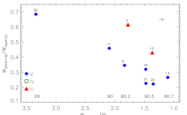
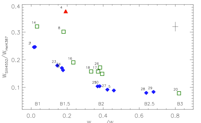
The photometric calibrations discussed in Sect. 4 depend on luminosity classifications of the star sample. Here, we re-examine their luminosity and spectral classification. As reference, we adopt the classification of one anchor point of the Morgan-Keenan system (star #11) and five primary standards from N. Walborn (#6, 7, 11, 19 and 23), all listed in Gray & Corbally (2009). In a second step, spectral types and luminosity classes of the sample stars are examined via inspection of Balmer lines and silicon/helium ratios, as recommended by Walborn (1971) and Gray & Corbally (2009). Spectral type classification for the hotter stars (O9-B0.7) rely on the ratio Si iv4089/Si iii4552 and for the cooler stars (B1-B3) on Si ii4128/Si iii4552. In addition, luminosity classes are tested via Si iv4116/He i4121 for the hotter and Si iii4552/He i4387 for the cooler stars.
Figure 11 displays the relation of line ratios as spectral type and luminosity class indicators for the hotter (upper panel) and the cooler stars (lower panel). Only few cases – stars #2, 8, 10, 19 and 26 – required a correction in luminosity class. Furthermore, slight corrections to (sub-)spectral types for objects #2, 5, 8, 10, 13, 16, 28, 29, have also been implemented, as listed in Table 1. The revisions are facilitated by the higher quality of our spectra in comparison to older photographic spectrograms used in the past, affecting in particular the weaker silicon lines. Star #15 is too cool, i.e. has a very low Si ii4128/Si iii4552 ratio, therefore is excluded from Figure 11 (lower panel).
Appendix B Spectroscopic indicators for temperature and surface determination
Table 4 indicates which ionization equilibria in combination with fits to several hydrogen lines, have been matched in order to determine effective temperatures and surface gravities for the sample stars. Dots denote fits to spectral lines and boxes indicate cases where ionization equilibria were matched. A row denotes the simultaneous fits to different elements/ionization stages using the same set of atmospheric parameters.
| HD | H | He i | He ii | C ii | C iii | C iv | O i | O ii | Ne i | Ne ii | Si iii | Si iv | Fe ii | Fe iii | ||
|---|---|---|---|---|---|---|---|---|---|---|---|---|---|---|---|---|
| 103 K | ||||||||||||||||
| 1 | 36591 | 27.0 | ||||||||||||||
| 2 | 61068 | 26.3 | ||||||||||||||
| 3 | 63922 | 31.2 | ||||||||||||||
| 4 | 74575 | 22.9 | ||||||||||||||
| 5 | 122980 | 20.8 | ||||||||||||||
| 6 | 149438 | 32.0 | ||||||||||||||
| 7 | 886 | 22.0 | ||||||||||||||
| 8 | 29248 | 22.0 | ||||||||||||||
| 9 | 35299 | 23.5 | ||||||||||||||
| 10 | 35708 | 20.7 | ||||||||||||||
| 11 | 36512 | 33.4 | ||||||||||||||
| 12 | 36822 | 30.0 | ||||||||||||||
| 13 | 36960 | 29.0 | ||||||||||||||
| 14 | 205021 | 27.0 | ||||||||||||||
| 15 | 209008 | 15.8 | ||||||||||||||
| 16 | 216916 | 23.0 | ||||||||||||||
| 17 | 3360 | 20.7 | ||||||||||||||
| 18 | 16582 | 21.2 | ||||||||||||||
| 19 | 34816 | 30.4 | ||||||||||||||
| 20 | 160762 | 17.5 | ||||||||||||||
| 21 | 37020 | 30.7 | ||||||||||||||
| 22 | 37042 | 29.3 | ||||||||||||||
| 23 | 36959 | 26.1 | ||||||||||||||
| 24 | 37744 | 24.0 | ||||||||||||||
| 25 | 36285 | 21.7 | ||||||||||||||
| 26 | 35039 | 19.6 | ||||||||||||||
| 27 | 36629 | 20.3 | ||||||||||||||
| 28 | 36430 | 19.3 | ||||||||||||||
| 29 | 35912 | 19.0 | ||||||||||||||
| 30 | 46202 | 34.1 | ||||||||||||||