Sparse Seismic Imaging using Variable Projection

Abstract

We consider an important class of signal processing problems where the signal of interest is known to be sparse, and can be recovered from data given auxiliary information about how this data was generated. For example, a sparse green’s function may be recovered from seismic experimental data using sparsity optimization when the source signature is known. Unfortunately, in practice this information is often missing, and must be recovered from data along with the signal using deconvolution techniques.

In this paper, we present a novel methodology to simultaneously solve for the sparse signal and auxiliary parameters using a recently proposed variable projection technique. Our main contribution is to combine variable projection with sparsity promoting optimization, obtaining an efficient algorithm for large-scale sparse deconvolution problems. We demonstrate the algorithm on a seismic imaging example.

Index Terms—  Sparsity optimization, variable projection, seismic imaging

1 Introduction

Sparse regularization has proven to be an indispensable tool in many areas, including inverse problems [1] and compressive sensing [2, 3]. If a signal $y$ is known to have a sparse or compressible (quickly decaying) representation $y=Sx$, this information can be used to formulate optimization problems of the form

$$\min\|x\|_{1}\quad\text{s.t.}\quad\|ASx-b\|_{2}^{2}\leq\sigma^{2},$$ (1)

where $A$ is a measurement matrix used to measure the true signal $y$, $b$ is a vector of data, and $\sigma$ is a threshold that depends on the characteristics of measurement error. In compressive sensing, it is possible to obtain recovery guarantees given properties of the true signal and $A$. In more general inverse problems, these guarantees have not been found; it is therefore appropriate to consider (1) as a regularization approach to the least squares problem. For example, in the seismic setting, where (1) has been particularly useful [4], $A$ is a linearized Born-scattering operator, $S$ is the curvelet transform, and $b$ is seismic data. While there are several popular algorithms that solve (1), e.g. SPArsa [5], the SPG$\ell_{1}$ [6] algorithm has been particularly useful for seismic imaging [7, 8, 9].

Many inverse problems contain unknown nuisance parameters that must be estimated in order to recover the solution [10]. In seismic imaging, the source wavelet is typically unknown. The main contribution of this paper is to extend the approach of [10] to the sparse inversion context, and derive simple modifications of standard sparse solvers to incorporate solutions of unknown nuisance parameters on the fly.

The paper proceeds as follows. In section 2, we introduce the seismic imaging problem with unknown wavelet, and formulate it as an extended sparsity promoting optimization problem (3). In section 3, we review the ideas recently proposed in [10] that allow nuisance parameters to be estimated on the fly, and show how to incorporate these ideas into existing sparsity promoting formulations. In section 4, we develop an extended SPG$\ell_{1}$ algorithm to solve (3), and we present numerical results in section 5.

2 Imaging with Unknown Wavelet

Seismic imaging is an approach to obtain a gridded subsurface velocity perturbation $y$ from seismic data, given a smooth starting model. Experiments are conducted by placing explosive sources on the surface and recording the reflected waves with an array of receivers on the surface. The data, $d_{i}$, in this case represents the Fourier transform of the recorded time series for frequency $i$. The corresponding modeling operator, $F_{i}$, defines a linear relation between the recorded data for the $i^{\mathrm{th}}$ frequency and the velocity perturbation. The statistical model for data given $y$ is

$$d_{i}=\alpha_{i}F_{i}y+\epsilon_{i},$$ (2)

where $\epsilon_{i}$ is a statistical model for the measurement error, which is typically modeled as Gaussian, and $\alpha_{i}$ are unknown complex source wavelet coefficients. Note that the model (2) is no longer linear in the decision variables $(x,\alpha)$—it is bilinear. Since the perturbation $y$ is known to be sparse in the Curvelet frame $C$, formulation (1) has been successfully used to recover $y=Cx$ [4] when the source wavelet is known. In full generality, the joint inverse problem for the perturbation $y$ and wavelet $\alpha$ is given by

$$\min_{x,\alpha}\|x\|_{1}\quad\text{s.t}\quad\sum_{i}\|d_{i}-\alpha_{i}F_{i}Cx\|_{2}^{2}\leq\sigma^{2}.$$ (3)

Note that the $\alpha$ parameters make the problem more difficult, because the forward model (2) is no longer linear in the decision variables $(x,\alpha)$, and the problem (3) is nonconvex.

3 Variable Projection

We begin by considering the problem

$$\min_{x,\alpha}\sum_{i}\|d_{i}-\alpha_{i}F_{i}Cx\|_{2}^{2}\quad\text{s.t.}\quad\|x\|_{1}\leq\tau\;.$$ (4)

The relationship between (4) and (3) will be fully explained in section 4. In this section, we show how to use results from [10] to design an effective algorithm for (4).

If we define ${\mathcal{X}}=\{x:\|x\|_{1}\leq\tau\}$, problem (4) is of the form

$${\mathcal{P}}\quad\min_{x\in{\mathcal{X}},\alpha}g(x,\alpha)\;,$$ (5)

where for any given $x\in{\mathcal{X}}$, one can easily find

$$\bar{\alpha}(x)=\operatorname*{argmin}_{\alpha}g(x,\alpha)\;.$$ (6)

In fact, $\bar{\alpha}(x)$ is available in closed form when the least squares penalty is used in (4). The key idea in [10] is to consider the modified objective

$$\tilde{g}(x)=g(x,\bar{\alpha}(x)),$$ (7)

using the convenient formula

$$\nabla_{x}\tilde{g}(\bar{x})=\nabla_{x}g(\bar{x},\bar{\alpha}(\bar{x})).$$ (8)

This is basically a generalization of the variable projection algorithm  [11].

In the current setting this means that instead of solving (4), we can simply solve the modified problem

$$\min_{x}\sum_{i}\|d_{i}-\bar{\alpha}_{i}(x)F_{i}Cx\|_{2}^{2}\quad\text{s.t.}\quad\|x\|_{1}\leq\tau$$ (9)

using e.g. the projected gradient iteration

$$x^{k+1}=P_{{\mathcal{X}}}[x_{k}-\alpha_{k}\nabla_{x}\tilde{g}(\bar{x}^{k})]$$

with $\nabla_{x}\tilde{g}$ computed via (8), with $\bar{\alpha}(x)$ given by (6). By [10, Corollary 2.3], a stationary point of (9) is also stationary point of (4).

4 Projected Regularized Inversion

In the previous section, we showed how to solve the extended problem (4). However, the formulation (3) is more important to us from the modeling perspective, since it is always easier to provide a noise threshold $\sigma$ than to figure out the ‘right’ sparsity level $\tau$. In fact, the SPG$\ell_{1}$ algorithm solves formulation (1) by solving a series of subproblems that find the sparsity level $\tau$ automatically given an input threshold $\sigma$.

In this section, we extend this approach to the pair of problems (3) and (4). First, define

$$v(\tau)=\min_{x,\alpha}\sum_{i}\|d_{i}-\alpha_{i}F_{i}Cx\|_{2}^{2}\quad\text{s.t.}\quad\|x\|_{1}\leq\tau$$ (10)

Suppose we find $\bar{\tau}$ such that $v(\bar{\tau})=\sigma^{2}$. Can we expect that the corresponding minimizers of (4) coincide with the minimizers of (3)? This question is answered in surprising generality by [12, Theorem 2.1]: as long as any minimizer $\bar{x}$ of (3) satisfies $\sum_{i}\|d_{i}-\alpha_{i}F_{i}C\bar{x}\|_{2}^{2}=\sigma^{2}$, then the set of minimizers of $\eqref{EBPDN}$ and $\eqref{ELASSO}$ match, and $\|\bar{x}\|_{1}=\bar{\tau}$ where $v(\bar{\tau})=\sigma^{2}$.

This general result points to using the following strategy: solve $v(\tau)=\sigma^{2}$ by Newton’s method

$$\tau^{k+1}=\tau_{k}-\frac{v(\tau_{k})-\sigma^{2}}{v^{\prime}(\tau_{k})}\;.$$ (11)

This is in fact the strategy used by SPG$\ell_{1}$ to solve the problem (1), for an appropriately defined value function. In order to implement this strategy, we have to be able to evaluate both $v(\tau)$ and $v^{\prime}(\tau)$ for (10).

Evaluating $v(\tau)$ is straightforward: we simply use the projected gradient method detailed in section 3. However, $v^{\prime}(\tau)$ is more difficult, since the most general variational results for value functions [12] require linearity of the forward model, which is violated by (2). Nonetheless, if we treat $\bar{\alpha}_{i}:=\bar{\alpha}_{i}(\bar{x})$ as fixed, then by [12, Theorem 6.2], we get

$$v^{\prime}(\tau)\approx-\left\|\sum_{i}\bar{\alpha}_{i}C^{T}F_{i}^{T}(d_{i}-\bar{\alpha}_{i}F_{i}C\bar{x})\right\|_{\infty}$$

where $\bar{x}$ solves (4) for $\tau$.

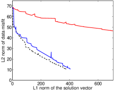
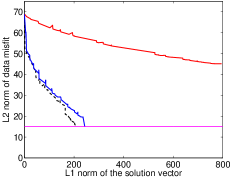
We note that the expression above is an approximation to the derivative, and the quality of the approximation remains to be determined. If the source weight can be estimated fairly quickly (so that it is not changing significantly between iterations), the approximation above becomes exact. For the experiments in the next section, we found that the proposed Newton iteration gives nearly the same result as the one with a fixed, ‘true’ source-weight. We also verified that when we pick $\sigma$ that is reachable within our computational budget of 150 iterations, the algorithm correctly finds the root $v(\tau)=\sigma$; see figure 4 (b).

5 Numerical Results

For the experiments we use a Matlab framework for seismic imaging and modelling [13], and the CurveLab toolbox [14]. Both of these are freely available for non-commercial purposes. The algorithm to solve 3 is based on the SPG$\ell_{1}$ code [15], which is also available for download.

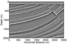
We generate data for the velocity perturbation defined on a 201 x 301 grid with 10 m spacing depicted in figure 1 for 6 frequencies between 5 and 25 Hz, 301 equispaced receivers and 15 composite sources, all located at the top of the model. We note that his leads to a underdetermined problem with 27090 equations and 60501 unknowns. We use SPG$\ell_{1}$ to solve (3) either with $\alpha$ fixed or with $\alpha$ estimated using the procedure outlined above. Since there is no noise in this example we use $\sigma=0$ and run the algorithm for a fixed number of iterations (100 in this case).

Note that there is a fundamental non-uniqueness in the problem; if we multiply the source-weights with a constant factor, we can compensate for this by dividing the reconstructed model by the same factor. Therefore, we normalize the results such that the source-weights for each reconstruction have the same norm (i.e., $\sum_{i}\bar{\alpha}_{i}(x)^{2}$ is the same for all reconstructions).

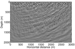
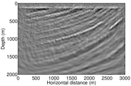
The reference result using the true source signature is shown in figure 2 (a). If we do not estimate the source signature and use $\alpha_{i}=1$, we do not get a good reconstruction, as is shown in figure 2 (b). Finally, if we estimate the source signature according to the strategy outlined in this paper, we obtain the result depicted in figure 2 (c).

The (normalized) optimal source weights $\bar{\alpha}(x)$ evaluated at the final results as well as the true source weight are depicted in figure 3. This shows that our approach is able to recover both the model and the source weight. The convergence histories of the SPG$\ell_{1}$ algorithm are shown in figure 4.

6 Discussion and Conclusions

We have proposed a novel method for estimating nuisance parameters in the context of sparsity regularized inverse problems, and in particular we have focused on source wavelet estimation in seismic imaging. The method draws on the idea of variable projection in order to estimate nuisance parameters on the fly, and can be implemented via a straightforward modification to existing sparse solvers.

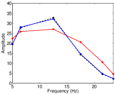
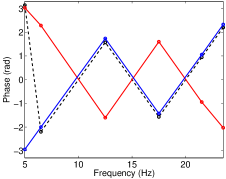
Numerical experiments demonstrate that the source wavelet can be recovered successfully in this manner (figure 3), and that the recovery of primary parameters (specifically of the image) is improved when the wavelet is estimated (figure 2).

Note that after section 3, we can already solve (4), but nonetheless lot of effort is devoted in section 4 to develop a method for solving (3). The main point here is that while it is difficult to come up with a reasonable value for $\tau$ in (4), it is straightforward to come up with a good value for $\sigma^{2}$ in (3). In fact, given a finite computational budget, and no estimate for $\sigma^{2}$, one can always pick $\sigma^{2}=0$ and perform a fixed number of iterations. In this mode, the algorithm in section 4 solves several (4) problems inexactly, picking the corresponding sequence of $\tau$ values according to iteration (11). This is exactly what was done to obtain the numerical examples in section 5.

Fig. 1: True perturbation used for numerical experiment

(a)

(b)

(c)

Fig. 2: Reconstructed models for the true wavelet (a), a wrong wavelet (b) and using the wavelet estimation procedure (c).

(a)

(b)

Fig. 3: Amplitude (a) and phase (b) of the optimal source weights evaluated at the models depicted in 2 (b) (red) and 2 (c) (blue). The true source weight is also shown (dashed line).

(a)

(b)

Fig. 4: Convergence histories using the true wavelet (dashed), a wrong source weight (red) and the estimated source weight (blue) when (a) $\sigma=0$ and (b) $\sigma=15$.

References

- [1] Felix J. Herrmann, Peyman P. Moghaddam, and Chris C. Stolk, “Sparsity- and continuity-promoting seismic imaging with curvelet frames,” Journal of Applied and Computational Harmonic Analysis, vol. 24, no. 2, pp. 150–173, 2008, doi:10.1016/j.acha.2007.06.007.
- [2] D. L. Donoho, “Compressed sensing,” IEEE Transactions on Information Theory, vol. 52, no. 4, pp. 1289–1306, 2006.
- [3] E. J. Candès, L. Demanet, D. L. Donoho, and L. Ying, “Fast discrete curvelet transforms,” Multiscale Modeling and Simulation, vol. 5, pp. 861–899, 2006.
- [4] Aleksandr Y. Aravkin, Xiang Li, and Felix J. Herrmann, “Fast seismic imaging for marine data,” in ICASSP. ICASSP, 2012, ICASSP.
- [5] S.J. Wright, R.D. Nowak, and M.A.T. Figueiredo, “Sparse reconstruction by separable approximation,” Signal Processing, IEEE Transactions on, vol. 57, no. 7, pp. 2479 –2493, july 2009.
- [6] E. van den Berg and M. P. Friedlander, “Probing the pareto frontier for basis pursuit solutions,” SIAM Journal on Scientific Computing, vol. 31, no. 2, pp. 890–912, 2008.
- [7] Felix Herrmann, Michael Friedlander, and Ozgur Yilmaz, “Fighting the Curse of Dimensionality: Compressive Sensing in Exploration Seismology,” IEEE Signal Processing Magazine, vol. 29, no. 3, pp. 88–100, May 2012.
- [8] Felix J. Herrmann and Xiang Li, “Efficient least-squares imaging with sparsity promotion and compressive sensing,” Geophysical Prospecting, vol. 60, no. 4, pp. 696–712, 2012.
- [9] Xiang Li, Aleksandr Y. Aravkin, Tristan van Leeuwen, and Felix J. Herrmann, “Fast randomized full-waveform inversion with compressive sensing,” Geophysics, vol. 77, no. 3, pp. A13–A17, 2012.
- [10] Aleksandr Y Aravkin and Tristan van Leeuwen, “Estimating nuisance parameters in inverse problems,” Inverse Problems, vol. 28, no. 11, pp. 115016, 2012.
- [11] G Golub and V Pereyra, “Separable nonlinear least squares: the variable projection method and its applications,” Inverse Problems, vol. 19, no. 2, pp. R1, 2003.
- [12] Aleksandr Y. Aravkin, James V. Burke, and Michael P. Friedlander, “Variational properties of value functions,” submitted to SIAM J. Optimization, arXiv:1211.3724, 2012.
- [13] T. van Leeuwen, “A parallel matrix-free framework for frequency-domain seismic modelling, imaging and inversion in matlab,” 2012, https://www.slim.eos.ubc.ca/releases.
- [14] David Donoho Lexing Ying Emmanuel Candes, Laurent Demanet, “CurveLab,” 2006, http://www.curvelet.org/.
- [15] E. van den Berg and M. P. Friedlander, “SPGL1: A solver for large-scale sparse reconstruction,” June 2007, http://www.cs.ubc.ca/labs/scl/spgl1.