Numerically Exact Long Time Magnetization Dynamics at the Nonequilibrium Kondo Crossover of the Anderson Impurity Model

Abstract

We investigate the dynamical and steady-state spin response of the nonequilibrium Anderson model to magnetic fields, bias voltage, and temperature using a numerically exact method combining a bold-line quantum Monte Carlo technique with the memory function formalism. We obtain converged results in a range of previously inaccessible regimes, in particular the crossover to the Kondo domain. We provide detailed predictions for novel nonequilibrium phenomena, including non-monotonic temperature dependence of observables at high bias voltage and oscillatory quench dynamics at high magnetic fields.

Strongly correlated open quantum systems appear in a wide variety of physical situations, including quantum dots in semiconductor heterostructures Goldhaber-Gordon et al. (1998); Hanson et al. (2007), molecular electronics Park et al. (2002); Heath and Ratner (2003) and the dynamics of cold atoms Brantut et al. (2012). These systems consist of a finite, interacting region coupled to a continuous set of non-interacting “bath” or “lead” states which may be maintained at differing thermodynamic states in such a way that no equilibrium state can exist. It is natural to describe open systems in terms of quantum impurity models, which have been used in the description of magnetic impurities in metals Anderson (1961), the adsorption of atoms on a surface Brako and Newns (1981) and as auxiliary problems in the dynamical mean field approximation to extended lattice systems Georges et al. (1996). More recently, they have also been of interest in the nonequilibrium context of mesoscopic transport Meir et al. (1993); Rosch et al. (2001) and nano-systems coupled to broad leads Hanson et al. (2007).

While attempts are being made to connect nonequilibrium physics to equilibrium concepts Dutt et al. (2011), the nonequilibrium steady state properties of correlated quantum systems continue to present a formidable challenge to our theoretical understanding. The main difficulty is that a rigorous evaluation of the long-time and steady state properties requires an accurate time propagation, starting from some known initial state and reaching all the way to the steady state. When this relaxation occurs quickly, a range of powerful semi-analytical Langreth and Nordlander (1991); Fujii and Ueda (2003); Eckstein et al. (2009) and numerical methods Mühlbacher and Rabani (2008); Bulla et al. (2008); Anders (2008); Werner et al. (2009); Schiró and Fabrizio (2009); Heidrich-Meisner et al. (2009); Gull et al. (2011a); Cohen and Rabani (2011) are applicable. However, dynamics in strongly correlated systems may exhibit a separation of timescales—for example, the spin-relaxation dynamics in the Kondo regime of a quantum dot are orders of magnitude slower than those of the corresponding charge relaxation. Existing theoretical methods are unable to resolve these timescales reliably.

In this Letter we show that a combination of bold-line diagrammatic Monte Carlo methods Gull et al. (2010, 2011a) and the memory-function approach Cohen and Rabani (2011) enables us to significantly extend the time regime accessible and can, in some cases, access steady state information within the Kondo regime. The method is numerically exact and provides unbiased error estimates. While the calculations presented here for the single impurity Anderson model, a minimal model for strong interactions in the presence of baths, the methodology is applicable to any quantum impurity model.

The Anderson impurity model is defined by the Hamiltonian

$$H=H_{S}+H_{B}+V,$$ (1)

where $H_{S}$ describes the interacting system (or dot) part, $H_{B}$ the non-interacting bath (or leads) part, and $V$ the system–bath coupling part:

$$H_{S} = \sum_{i=\uparrow\downarrow}\varepsilon_{i}d_{i}^{\dagger}d_{i}+Ud_{\uparrow}^{\dagger}d_{\uparrow}d_{\downarrow}^{\dagger}d_{\downarrow},$$ (2)

$$H_{B} = \sum_{k,i=\uparrow\downarrow}\varepsilon_{ik}a_{ik}^{\dagger}a_{ik},$$ (3)

$$V = \sum_{k,i=\uparrow\downarrow}t_{ik}d_{i}a_{ik}^{\dagger}+t_{ik}^{*}a_{ik}d_{i}^{\dagger}.$$ (4)

Here $\uparrow$ and $\downarrow$ represent electronic spin, the $d_{i}$ and $d_{i}^{\dagger}$ are fermionic system operators for dot states with energy $\varepsilon_{i}$, $a_{ik}$ and $a_{ik}^{\dagger}$ are fermionic lead operators with energy $\varepsilon_{ik}$ and the $t_{ik}$ are coupling constants. $k$ is an index iterating over the lead states. Both the $\varepsilon_{ik}$ and the $t_{ik}$ are fully defined by the system–lead coupling density $\Gamma\left(\varepsilon\right)\equiv 2\pi\sum_{k}\left|t_{k}\right|^{2}\delta\left(\varepsilon-\varepsilon_{ik}\right)$.

Refs. Nakajima (1958); Zwanzig (1960); Mori (1965) have shown that the reduced density matrix $\sigma\left(t\right)=\mathrm{Tr}_{B}\left\{\rho\left(t\right)\right\}$ ($\rho\left(t\right)$ being the full density matrix and $\mathrm{Tr}_{B}\left\{...\right\}$ denoting a trace over all bath degrees of freedom) of any system of the form of Eq. (1) exactly obeys the Nakajima–Zwanzig–Mori equation

$$i\hbar\frac{\mathrm{d}\sigma\left(t\right)}{\mathrm{d}t}=\mathcal{L}_{H_{S}}\sigma\left(t\right)+\vartheta\left(t\right)-\frac{i}{\hbar}\int_{0}^{t}\mathrm{d}\tau\,\kappa\left(\tau\right)\sigma\left(t-\tau\right).$$ (5)

Here, the Liouvillian superoperator $\mathcal{L}_{H_{S}}A\equiv\left[H_{S},A\right]$ denotes a commutation with the system Hamiltonian $H_{S}$, with the same notation defining $\mathcal{L}_{V}$ and $\mathcal{L}_{H}$; $\vartheta\left(t\right)$ is an initial correlation term which vanishes for factorized initial conditions $\rho\left(0\right)\equiv\rho_{B}\otimes\sigma\left(0\right)$; and $\rho_{B}$ is the initial bath density matrix. $\kappa$ is known as the memory kernel and may be obtained by solving Zhang et al. (2006)

$$\kappa\left(t\right) = i\hbar\dot{\Phi}\left(t\right)-\Phi\left(t\right)\mathcal{L}_{S}+\frac{i}{\hbar}\int_{0}^{t}\mathrm{d}\tau\Phi\left(t-\tau\right)\kappa\left(\tau\right),$$ (6)

where the superoperator $\Phi\left(t\right)\equiv\mathrm{Tr}_{B}\left\{\mathcal{L}_{V}e^{-\frac{i}{\hbar}\mathcal{L}_{H}t}\rho_{B}\right\}$ must in general be obtained from a many body computation whose expense rapidly increases as $t$ increases. Evaluation of $\Phi\left(t\right)$ for $t$ up to a cutoff time $t_{c}$ allows an exact evaluation of $\kappa\left(t<t_{c}\right)$. Setting $\kappa\left(t>t_{c}\right)=0$ defines the cutoff approximation, whose convergence may be monitored from the dependence of results on $t_{c}$ as $t_{c}$ is increased. In the case of the Anderson impurity model, Ref. Cohen and Rabani (2011) has shown that if one is only interested in evaluating the diagonal elements of the density matrix, all the supermatrix elements $\Phi_{ij,qq^{\prime}}\equiv\left(\left|i\right\rangle\left\langle j\right|\right)^{\dagger}\Phi\left|q\right\rangle\left\langle q^{\prime}\right|$ of $\Phi$ having $i\neq j$ or $q\neq q^{\prime}$ can be set to zero, with the remaining elements determined by:

$$\Phi_{ii,qq} = \delta_{i0}\left(\varphi_{qq}^{\left(1\right)}+\varphi_{qq}^{\left(3\right)}\right)+\delta_{i1}\left(\varphi_{qq}^{\left(2\right)}-\varphi_{qq}^{\left(3\right)}\right)$$ (7)

$$+ \delta_{i2}\left(-\varphi_{qq}^{\left(1\right)}+\varphi_{qq}^{\left(4\right)}\right)+\delta_{i3}\left(-\varphi_{qq}^{\left(2\right)}-\varphi_{qq}^{\left(4\right)}\right),$$

$$\varphi_{qq}^{\left(m\right)}\left(t\right) = 2i\Im\sum_{k}\mathrm{Tr}_{B}\left\{\rho_{B}\left\langle q\right|A_{k}^{\left(m\right)}\left(t\right)\left|q\right\rangle\right\},$$ (8)

where $A_{k}^{\left(1\right)}=t_{\uparrow k}d_{\uparrow}d_{\downarrow}d_{\downarrow}^{\dagger}a_{\uparrow k}^{\dagger}$, $A_{k}^{\left(2\right)}=t_{\uparrow k}d_{\uparrow}d_{\downarrow}^{\dagger}d_{\downarrow}a_{\uparrow k}^{\dagger}$, $A_{k}^{\left(3\right)}=t_{\downarrow k}d_{\uparrow}d_{\uparrow}^{\dagger}d_{\downarrow}a_{\downarrow k}^{\dagger}$ and $A_{k}^{\left(4\right)}=t_{\downarrow k}d_{\uparrow}^{\dagger}d_{\uparrow}d_{\downarrow}a_{\downarrow k}^{\dagger}$.

The evaluation of the $\varphi_{qq}^{\left(m\right)}\left(t\right)$ has previously been performed with real time path integral Monte Carlo (RT-PIMC) methods Mühlbacher and Rabani (2008); Werner et al. (2008); Cohen and Rabani (2011), revealing that, in the presence of strong electronic correlations, the memory kernel may develop long tails. Near the Kondo regime this effect becomes particularly pronounced, making it impossible to converge the cutoff approximation and highlighting the need for methods able to obtain $\kappa$ for longer times. Here we show that the problem can to a large extent be solved by using the bold expansion for impurity models Gull et al. (2010), a technique related to bold-line methods for lattice systems Prokof’ev and Svistunov (2007, 2008); Van Houcke et al. (2012). The bold expansion is based on a stochastic Monte Carlo sampling of diagrammatic corrections to the propagators obtained from an infinite partial summation, rather than a sampling of all diagrams. The resulting procedure converges at lower expansion order and greatly reduces the severity of the dynamic sign problem, in practice more than doubling the accessible time scales. Even with bold methods, a direct description of the slow spin dynamics remains out of reach—however, the bold method does allow converged access to such dynamics within the memory formalism.

Figure 1: Self energies and vertex equations used within the OCA based bold expansion. Solid lines represent bare propagators, bold lines are dressed propagators, wavy lines are hybridization interactions and shaded regions are vertex functions. The vertices are defined on the unfolded Keldysh contour, such that the final time on the contour is marked by the central “X” and both edges of the contour stand for the initial time. The NCA is obtained by taking only the first diagram in the self energy and the first two diagrams in the vertex.

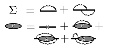
In the nonequilibrium case, diagrams must be evaluated on the Keldysh contour. This had previously been done with “BoldNCA”, using the non-crossing approximation (NCA) as the underlying partial summation, but in the course of this work it has become necessary to employ a “BoldOCA” built on the more precise one-crossing approximation (OCA) Gull et al. (2010); Pruschke and Grewe (1989). Fig. 1 illustrates this in diagrammatic terms: the bold-line propagators and vertex functions (which allow for the summation over hybridization lines connecting pairs of times on the two different halves of the Keldysh contour) are obtained from the solution of the NCA or OCA equations, and used in an expansion which samples diagrams of all crossing orders. Unbiased error estimates are obtained by jackknife analysis on data from multiple, uncorrelated Monte Carlo runs (typically 5–10).

We assume a wide, flat band $\Gamma_{i}\left(E\right)=\Gamma_{i}^{L}\left(E\right)+\Gamma_{i}^{R}\left(E\right)$ with $\Gamma_{i}^{L\left(R\right)}\left(E\right)=\frac{\Gamma/2}{\left(1+e^{\nu\left(E-\varepsilon_{c}\right)}\right)\left(1+e^{-\nu\left(E+\varepsilon_{c}\right)}\right)}$; here $\varepsilon_{c}$ and $\nu$ are the band cutoff energy and its inverse cutoff width, and $L$ and $R$ are respectively left and right lead indices. We restrict our calculations to the symmetric Anderson impurity model in a magnetic field $h$, setting $\varepsilon_{i}=-\frac{U}{2}\pm\frac{h}{2}$ (the formalism is more general and does not rely on this symmetry). We choose $\Gamma$ as our energy unit, and throughout the rest of this paper set $U=5\Gamma$, $\varepsilon_{c}=10\Gamma$ and $\Gamma\nu=10$. The initial conditions are determined by assuming an initially decoupled system, having left and right leads thermally equilibrated at a temperature $\beta$ and chemical potentials $\mu_{L}=\frac{V}{2}$ and $\mu_{R}=-\frac{V}{2}$, respectively. This defines the lesser and greater hybridization functions $\Delta_{L\left(R\right)}^{<}\left(\omega\right)=-if_{L\left(R\right)}\left(\omega\right)\Gamma_{L\left(R\right)}\left(\omega\right)$ and $\Delta^{>}\left(\omega\right)=i\left(1-f_{L\left(R\right)}\left(\omega\right)\right)\Gamma_{L\left(R\right)}\left(\omega\right)$, which depend on the temperature and chemical potentials through the Fermi occupation function $f_{L\left(R\right)}\left(\omega\right)=\frac{1}{1+e^{\beta\left(\omega-\mu_{L\left(R\right)}\right)}}$. At these parameters, the Kondo temperature is given by $\Gamma\beta_{K}\equiv\frac{\Gamma}{T_{K}}\simeq 3.4$ Hewson (1993).

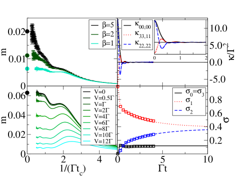
In equilibrium, the magnetization can be evaluated exactly on the Matsubara axis Werner et al. (2006); Gull et al. (2010, 2011b). As this magnetization corresponds to the steady state magnetization at zero bias voltage, it is useful as a benchmark. The top left panel of Fig. 2 displays the steady state magnetization predicted by the proposed method at $V=0$, plotted against the inverse cutoff time $\frac{1}{\Gamma t_{c}}$ at several temperatures. Comparing the predicted steady state to the equilibrium results (circles) shows that the cutoff approximation converges rapidly even as one crosses the edge of the Kondo regime. For the very small magnetic field $h=0.01\Gamma$ in Fig. 2, the relative errors are rather large, but considered on the full scale of the magnetization the precision demonstrated here is remarkable.

The effects of taking the system out of equilibrium are illustrated in the lower left panel of Fig. 2. Here a constant temperature $\beta\Gamma=1$ is maintained while the bias voltage $V$ is varied at $h=0.1\Gamma$; the numerically exact $V=0$ result is also shown. This plot clearly illustrates that convergence of the method generally occurs at even shorter times in nonequilibrium conditions—equilibrium exhibits the longest memory, consistent with expectations.

An independent approach to verifying convergence relies on direct examination of individual elements of the memory kernel as a function of time. Several representative elements are displayed at $h=0.01\Gamma$ and $\beta\Gamma=1$ in the top right panel of Fig. 2, with the inset highlighting short times. Within the times accessible by BoldOCA, the memory kernel elements go to zero within the numerical accuracy. Below this, on the same time scale and for the same parameters, the time dependence of the three distinct elements of the reduced density matrix $\sigma$ is plotted for an initially magnetized dot in the lower right panel of Fig. 2. With this initial condition and within the symmetric Anderson impurity model, the diagonal density matrix entries $\sigma_{0}$ and $\sigma_{3}$, which express charging dynamics, are identical. They both relax rapidly, and in fact their steady state values could have been obtained to very good accuracy within BoldNCA only. The difference in scale between the spin relaxation time of $\sigma_{1},\sigma_{2}$ and the memory decay in the upper panel, however, is striking—and is why our memory kernel methods are essential for obtaining long-time behavior. To obtain a reasonable converged steady state directly, one would need to reach times $\Gamma t\gtrsim 20$ with errors of similar magnitude compared to what we have obtained at $\Gamma t=2$ with the current approach. The exponential scaling in time typical of all general exact methods makes this unfeasible.

Figure 2: Top left panel: The steady-state magnetization obtained from the memory formalism at several temperatures plotted as a function of the inverse cutoff time, and compared in the equilibrium cases to exact CT-QMC results shown as circles, for $h=0.01\Gamma$ and $V=0$. Bottom left panel: The same plot at $\beta\Gamma=1$ and $h=0.1\Gamma$, for several voltages. Right panels: equilibrium memory kernel $\kappa$ (top) and populations $\sigma_{i}$ (bottom) as a function of time for $\beta\Gamma=1$ and $h=0.01\Gamma$. The inset shows the memory kernel at short times. The squares in the bottom right panel are approximate OCA results.

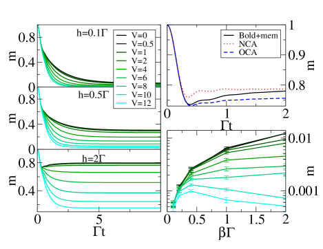
We now turn from the demonstration of convergence to presentation of results. The left panels of Fig. 3 show the time evolution of the magnetization from an initially polarized state at different voltages and magnetic fields, with $\beta\Gamma=1$. At low voltages two separate relaxation timescales are apparent: immediate fast relaxation followed by later slow relaxation. At high enough fields (bottom), an overshoot effect appears along with oscillatory behavior which is seen more clearly in the upper right panel. As we increase the voltage the second timescale is suppressed and eventually the relaxation becomes exponential. However, the voltage required in order to reach this regime is surprisingly large. In the top right panel of Fig. 3, we show that nonequilibrium NCA and OCA (not supplemented by QMC) do very poorly away from $h=0$ and cannot be considered reliable, whereas the memory approach and the underlying BoldOCA continue to converge very well.

In the lower right panel of Fig. 3, we show an example of the temperature dependence of the $t\rightarrow\infty$ limit of the magnetization at constant magnetic field and a range of bias voltages. Interestingly, at higher voltages (but substantially below $\frac{V}{2}\approx\omega_{c}$ where the lead chemical potentials approach the band cutoff) the temperature dependence becomes non-monotonic. We believe this is a population switching effect Cohen and Rabani (2008), which leads to a suppression of the magnetization by population transfer from the magnetized $\left|1\right\rangle$ and $\left|2\right\rangle$ states to the unmagnetized $\left|0\right\rangle$ and $\left|3\right\rangle$ states which are activated for $V\gtrsim U$. The rate for this transfer process is approximately proportional to the lead occupation at the energy difference between the states: $f\left(\beta,\Delta E,\mu\right)=\frac{1}{1+e^{\beta\left(\Delta E-\mu\right)}}$, with $\Delta E$ equal to half the interaction energy $\frac{U}{2}$ and $\mu=\frac{V}{2}$ or $-\frac{V}{2}$, depending on the lead. $f$ is therefore an increasing function of temperature for $V<U$ and a decreasing one for $V>U$. At small voltages the effect of the population transfer results in a reduction of the magnetization (as expected), while at large voltages the population transfer enhances the intermediate-temperature magnetization. At still larger temperatures, the nonequilibrium effects are washed away and normal thermal suppression of the magnetization occurs. A maximum can therefore be expected, as is indeed observed in the numerically converged calculations.

Figure 3: Left panels: Time dependence of the cutoff-converged magnetization at $\beta\Gamma=1$ starting from a fully magnetized dot, at different magnetic fields $h$ and bias voltages $V$. Top right: Comparison with NCA and OCA at $h=2\Gamma$ and $V=0$. Bottom right: Temperature dependence of the $h=0.01\Gamma$ steady state magnetization at different voltages.

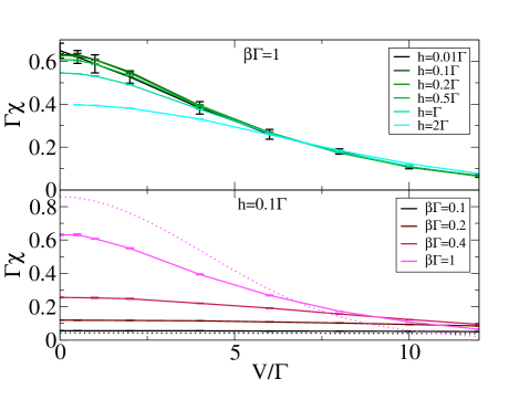
In Fig. 4 we display the steady state voltage dependence of the generalized magnetic susceptibility $\chi\equiv\frac{m}{h}$. At small $h$ this quantity is $h$-independent. The top panel shows clearly how the regime in which $m$ is linear in $h$ depends on voltage at a constant temperature. The bottom panel of Fig. 4 shows the voltage dependence at different temperatures within the linear regime. One immediately noticeable feature is the decrease of $\chi$ with increasing $\beta$ at high voltage, which corresponds to the non-monotonic temperature dependence discussed in the bottom panel of Fig. 4. A second interesting feature is the fact that the plots have a simple, Lorentzian-like structure, suggesting that the results may be in a regime accessible to analytical methods based on performing logarithmic corrections around rate equations Paaske et al. (2004): in the dotted lines in the bottom panel we show for comparison results obtained by solving the classical rate equations (obtained by simple perturbation theory to second order in the hybridization). The large discrepancy between the master equation and numerically exact results at $\beta\Gamma=1$ shows that in the crossover regime, even at large voltage a correct account of the physics requires accurate calculations of the sort performed here.

Figure 4: Generalized magnetic susceptibility $\chi\equiv\frac{m}{h}$ as a function of voltage, for (top) different magnetic fields and (bottom) different temperatures, at $h=0.1\Gamma$. Approximate results from a master equation calculation are shown in dotted lines for the lowest and highest temperatures in the lower panel.

In conclusion, by unifying numerically exact bold Monte Carlo methods with the exact memory approach we have developed a new, numerically exact formalism free from systematic errors and well suited for the real time solution of nonequilibrium quantum impurity models. In practice, the capabilities of this formalism are unparalleled: the method generates precise, converged results at all timescales, in cases where the current state-of-the-art approximate methods clearly fail. For the nonequilibrium Anderson impurity model, the formalism performs well even as one enters the Kondo regime, a regime previously inaccessible with accurate numerical methods.

Our formalism has allowed us to explore the detailed behavior of the nonequilibrium magnetization, and we have made predictions regarding multi-scale, oscillatory quenching dynamics at high magnetic fields; the effect of voltage on dynamical relaxation; and population-driven reversal of the magnetization’s temperature dependence at high voltages. These results are obtained at parameters where no other currently available method is reliable. As the temperature is further lowered, one expects to encounter the formation of Kondo peaks at the chemical potential. How this will affect the behavior described here remains an interesting and open question, and work is currently being carried out to further investigate this issue. Future research will address lower temperatures and a wider variety of observables; it is also worth stressing that both bold techniques and the memory formalism are not specific to the Anderson impurity model, and are expected to have many more applications.