Constraints on Dark Energy state equation with varying pivoting redshift

Abstract

We assume the DE state equations $w(a)=w_{0}+w_{a}(a_{p}-a)$, and study the dependence of the constraints on $w_{0}$ and $w_{a}$ coefficients on the pivoting redshift $1+z_{p}=1/a_{p}$. Coefficients are fitted to data including WMAP7, SNIa (Union 2.1), BAO’s (including WiggleZ and SDSS results) and $H_{0}$ constraints. The fitting algorithm is CosmoMC. We find specific differences between the cases when $\nu$–mass is allowed or disregarded. More in detail: (i) The $z_{p}$ value yielding uncorrelated constraints on $w_{0}$ and $w_{a}$ is different in the two cases, holding $\sim 0.25$ and $\sim 0.35$, respectively. (ii) If we consider the intervals allowed to $w_{0}$, we find that they shift when $z_{p}$ increases, in opposite directions for vanishing or allowed $\nu$–mass. This leads to no overlap between 1$\sigma$ intervals already at $z_{p}>\sim 0.4$. (iii) The known effect that a more negative state parameter is required to allow for $\nu$ mass displays its effects on $w_{a}$, rather than on $w_{0}$. (iv) The $w_{0}$–$w_{a}$ constraints found by using any pivot $z_{p}$ can be translated into constraints holding at a specific $z_{p}$ value (0 or the $z_{p}$ where errors are uncorrelated). When we do so, error ellipses exhibit a satisfactory overlap.

1 Introduction

Owing to the conceptual problems of $\Lambda$CDM, a number of options for Dark Energy (DE) nature have been considered. In particular, DE could be a scalar field, necessarily self–interacting and possibly interacting with Dark Matter (Damour et al., 1990; Wetterich, 1995; Amendola, 2000; Amendola & Quercellini, 2001; Dalal et al., 2001; Amendola & Tocchi Valentini, 2002; Mainini & Bonometto, 2004; Maccio’ et al., 2004; Mainini & Bonometto, 2006, 2007; Bento & Bortolami, 2009; Bento et al., 2008; Zimdahl et al., 2001; Del Campo & Herrera, 2006; Wei & Zhang, 2007; Amendola et al., 2007; Guo et al., 2007; Caldera-Cabral et al., 2009; Pettorino et al., 2012), or just a phenomenological consequence of large scale GR violations (Capozziello et al., 2006; Amendola et al., 2007; Creminelli et al., 2009; Park et al., 2010; Bloomfield & Flanagan, 2012). But neither these options, nor still more exhotic hypotheses (Tomita, 2000; Celerier, 2000; Tomita, 2001; Iguchi et al., 2002; Jimenez et al., 2012), led to appreciable improvements of the fit between theory and data (Colombo et al., 2009; Mainini, 2009; Kristiansen et al., 2010).

The problem has then been tackled from the phenomenological side, by testing whether any linear $w(a)$, different from $w(a)\equiv-1$, improves data fits. A possible option amounts then to express the linear laws through the equations

$$w(a)=w_{0}+w_{a}(1-a)~{},$$ (1)

aiming then at testing how various sets of data yield constraints on $w_{0}$ and $w_{a}$. Here $a$ is the scale factor, normalized to unity at the present time. In the literature, this expression for $w(a)$ was first used by Chevallier & Polarski (2001).

The same linear laws can be expressed also through the equations

$$w(a)=w_{0,a_{p}}+w_{a,a_{p}}(a_{p}-a)$$ (2)

which differ from (1) for selecting a non–vanishing pivoting redshift

$$z_{p}=1/a_{p}-1~{},$$ (3)

while we put an extra index to the linear coefficients $w_{0,a_{p}}$, $w_{a,a_{p}}$ to put in evidence that, when changing $z_{p}$, their values change. The straight lines defined by eq. (1) and eq. (2) are however the same: any equation (2) turns into an equation (1) if we set

$$w_{0,a_{p}}=w_{0}-w_{a}(a_{p}-1)$$ (4)

and $w_{a,a_{p}}=w_{a}$. Notice that this last identity does not imply that limits on $w_{a,a_{p}}$ are independent from the pivoting redshift. In the sequel, whenever this causes no confusion, we shall however follow the common use and call $w_{0}$, $w_{a}$ the two parameters in any expression (2).

Linear laws can be fitted to data by using different $a_{p}$ values. Here we aim at testing, first of all, how compatible are results obtained when varying the pivoting redshift.

We shall do so in two cases: either neglecting or allowing the option that $M_{\nu}=\sum_{\nu}m_{\nu}\neq 0$ (the sum is extended to the mass eigenvalues for 3 standard neutrino flavors). Let us also remind that the neutrino density parameter

$$\Omega_{\nu}h^{2}=1.08\times 10^{-2}(M_{\nu}/{\rm eV})(T_{0\gamma}/2.73\,\,{\rm K})^{3}~{},$$ (5)

so that, when the dark matter reduced density parameter $\omega_{c}=\Omega_{c}h^{2}$ is assigned, the neutrino fraction $f_{\nu}=\Omega_{\nu}/\Omega_{c}$ immediately follows.

The value of $a_{p}$ can be selected so to have uncorrelated phenomenological constraints on $w_{0}$ and $w_{a}$. Here we also wish to put in evidence that: (i) the pivoting redshift yielding uncorrelated constraints is different, if $f_{\nu}\equiv 0$ or can be $\neq 0$; (ii) also the dependence on $a_{p}$ of the $w_{0}$ interval compatible with data depends on the above option.

We expect that the DE state parameter $w$ takes lower values, even in the phantom domain, when $M_{\nu}$ is allowed. We shall test how this occurs, when we consider a wide set of data (see below). In particular, by allowing for (linearly) variable $w$, we can test whether data require a constantly low $w_{0}$ or a progressively decreasing law, set by a negative $w_{a}$.

Figure 1: 2D marginalized likelihood, when taking $z_{p}=0$, on the plane $w_{0}-w_{a}$ at 65% and 95% of confidence for different data sets, when assuming massless (l.h.s.) or massive (r.h.s.) neutrinos. The coordinate scale being the same on both sides allows us to appreciate how the $w_{0}$–$w_{a}$ uncertainty increases when a $\nu$–mass degree of freedom is considered.

In the recent literature, the set of linear $w(a)$ has also been parametrized by using the values taken by $w$ at $z=0$ and at a higher redshift, e.g. $z=0.5~{}.$ In spite of advantages of this parametrization (Wang (2008)), quite a few authors still keep to the old one. We plan to deepen the relation with such approach in further work.

2 Results for $z_{p}=0$.

Let us then report, first of all, the results of Monte Carlo fits of DE state equations vs. data, performed by using the algorithm CosmoMC (Lewis et al. (2002), May 2010 version); the CosmoMC code was integrated with the first version of the PPF module for CAMB (Lewis et al. (2000), Fang et al. (2008)). Fits were performed in respect to the following parameters: $w_{0}$, $w_{a}$ (in eq. 2) and $\omega_{b}=\Omega_{b}h^{2}$, $\omega_{c}=\Omega_{c}h^{2}$, $\theta=100~{}l_{s}/l_{d}$, $\tau$, $n_{s}$, $\log A$, $A_{SZ}$, plus $f_{\nu}$ when needed (respectively: reduced baryon density parameter, reduced CDM density parameter, 100 times the ratio between sound horizon at recombination and its angular diameter distance, optical depth due to reionization, primeval spectral index, logarithmic fluctuation amplitude with pivoting scale $0.05\,\,$Mpc^-1, SZ template normalization, neutrino fraction as defined below; $h$ is the Hubble parameter in units of 100 (km/s)/Mpc). We however kept $\Omega_{k}=0$.

Our data set includes CMB data from WMAP7, supernovae from Union2.1 survey (Suzuki et al. (2012), option with no systematic errors), WiggleZ and SDSS BAO’s data (Blake et al. (2011), Percival et al. (2010)), HST data (Riess et al. (2009)) and CMB lensing as provided by CosmoMC. We use different combinations of these data, as suitably detailed below.

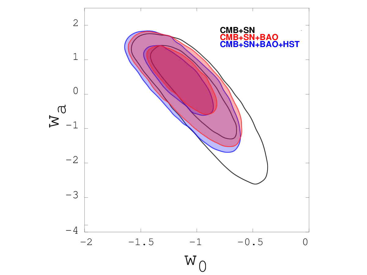
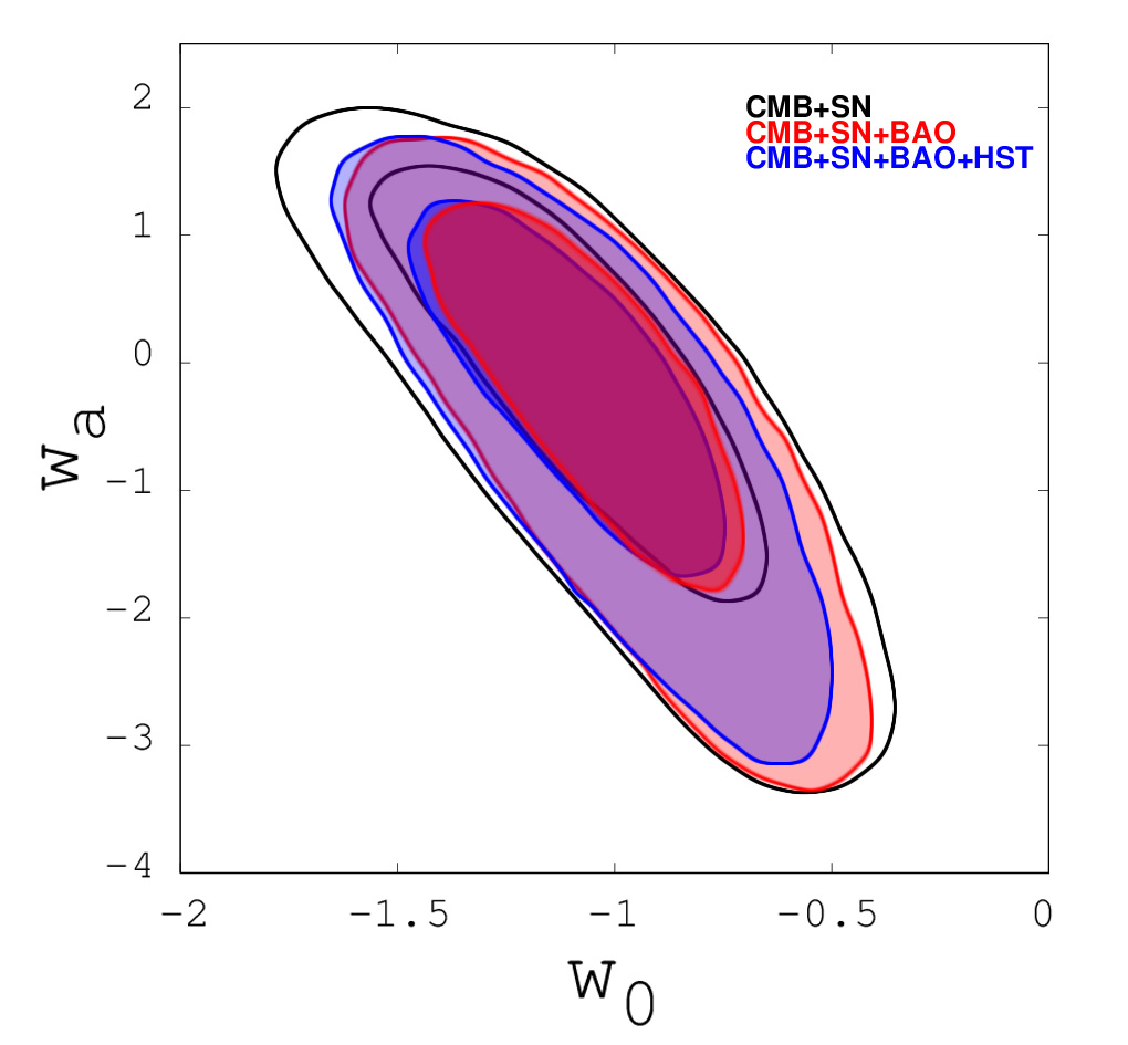
In Figure 1 we show $1\sigma$ and $2\sigma$ contours for the marginalized likelihood on the $w_{0}$–$w_{a}$ plane, when $z_{p}=0$, for the sets of data indicated in the frame. In comparison with the analogous curves shown in WMAP7 report Komatsu et al. (2011) for $f_{\nu}=0$, our ellipses are slightly displaced towards more negative $w_{0}$ and greater $w_{a}$. The ranges found are closer to the Union 2.1 report by Suzuki et al. (2012).

To gauge the widening of $w_{0}$ and $w_{a}$ intervals when $M_{\nu}\neq 0$ is allowed, we kept the same abscissa and ordinate ranges in both sides. The widening is confirmed when fully marginalizing in respect to all other parameters, as is shown in Table 1. Let us however notice that, when $M_{\nu}\equiv 0$ is required, the inclusion of BAO and/or HST data in top of CMB, causes a displacement towards smaller values of the mean $w_{0}$ and an increase of $w_{a}$. These shifts –just below $1\sigma$– do not occur (or are much smaller) when $M_{\nu}\neq 0$ .

	Massless	Neutrinos	Massive	Neutrinos
Data Set	$w_{0}\pm 1\sigma\pm 2\sigma$	$w_{a}\pm 1\sigma\pm 2\sigma$	$w_{0}\pm 1\sigma\pm 2\sigma$	$w_{a}\pm 1\sigma\pm 2\sigma$	$f_{\nu}\pm 1\sigma\pm 2\sigma$
CMB+SN	$-0.99_{-0.13-0.36}^{+0.11+0.41}$	$-0.04_{-0.36-1.74}^{+0.56+1.25}$	$-1.06_{-0.14-0.45}^{+0.13+0.46}$	$-0.25_{-0.44-2.14}^{+0.68+1.56}$	$0.045_{-0.045-0.045}^{+0.013+0.052}$
….+BAO	$-1.10_{-0.10-0.30}^{+0.08+0.33}$	$~{}~{}~{}0.33_{-0.24-1.25}^{+0.37+0.92}$	$-1.03_{-0.12-0.35}^{+0.10+0.39}$	$-0.37_{-0.36-2.01}^{+0.60+1.41}$	$0.040_{-0.040-0.040}^{+0.011+0.043}$
….+HST	$-1.13_{-0.10-0.30}^{+0.09+0.33}$	$~{}~{}~{}0.29_{-0.25-1.30}^{+0.39+1.00}$	$-1.07_{-0.11-0.34}^{+0.10+0.38}$	$-0.31_{-0.34-1.89}^{+0.56+1.37}$	$0.036_{-0.036-0.036}^{+0.009+0.041}$

Table 1: Mean, $1\sigma$ limits and $2\sigma$ limits on $w_{0}$, $w_{a}$ and $f_{\nu}$ (when relevant), with and without massive neutrinos and different data sets. Values are obtained by fully marginalizing over all other parameters. As indicated, in the second line BAO data are added to CMB+SN data, in the third line also HST data are included. The pivoting redshift is however $z_{p}=0$.

Figure 2: 2D marginalized likelihood on the plane $f_{\nu}-w_{0}$ (l.h.s.) and $f_{\nu}-w_{a}$ (r.h.s.) at 65% and 95% of confidence for different data sets, obtained with $z_{p}=0$.

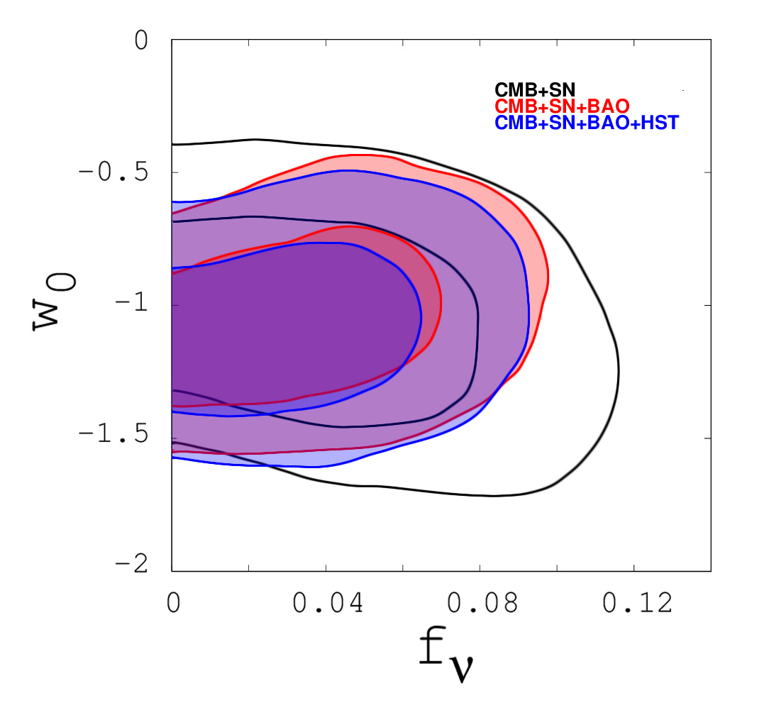
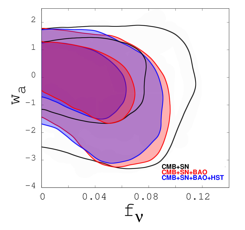
In Figure 2 we show the likelihood distributions on the $f_{\nu}$–$w_{0}$ and $f_{\nu}$–$w_{a}$ planes, outlining a progressive delving of $w_{a}$ into the negative domain when $f_{\nu}$ shifts from 0 to 0.04  (i.e., when $M_{\nu}$ shifts from 0 to $\sim 0.60~{}$eV). The known result that a greater $M_{\nu}$ is allowed, when $w$ delves in the phantom area, therefore affects $w_{a}$ rather than $w_{0}$, so indicating that, to soften $M_{\nu}$ limits, it seems preferable that $w$ shifts below -1 just when $z>0~{}.$

More in detail, if constant $w$ models only are considered, as in Komatsu et al. (2011) or De Bernardis et al. (2008), one finds that, to compensate a massive neutrino component, DE density fading more rapidly than in $\Lambda$CDM, as $z$ increases, is favored. As is known, even for $M_{\nu}\sim 0.1\,$eV, neutrino derelativization is complete before $z=100~{}.$ Since then, the whole linear fluctuation spectrum evolves $\propto(1+z)^{-1}$ until the spectral growth is slowed down by DE acquiring a significant density. If $w$ is constant and $<-1$, DE density becomes significant later than in $\Lambda$CDM; a later slow down compensates the spectral depression, which is one of the consequences of neutrino mass. For instance, De Bernardis et al. (2008) found a constant $w=-1.12\pm 0.09$. With our wider dataset, we found $w=-1.11^{+0.05}_{-0.04}$, an almost coincident result, apart of a halvened (1$\sigma$) errorbar.

When $w$ linear variations are allowed, errors become greater, as expected. The central point of $w_{0}$ ($\simeq-1.07$) however rises up to the 1$\sigma$ limit for constant–$w$ models, while $w$ tends to become negative because of $w_{a}.$ This means a different timing in the reduced slowing down. A natural guess is that data coming from the epoch when DE starts to become significant, e.g. WiggleZ data, are better fitted by an early spectrum not only higher than $\Lambda$CDM, but even higher than a $w\simeq-1.12$ phantom model.

3 Results for $z_{p}\neq 0$

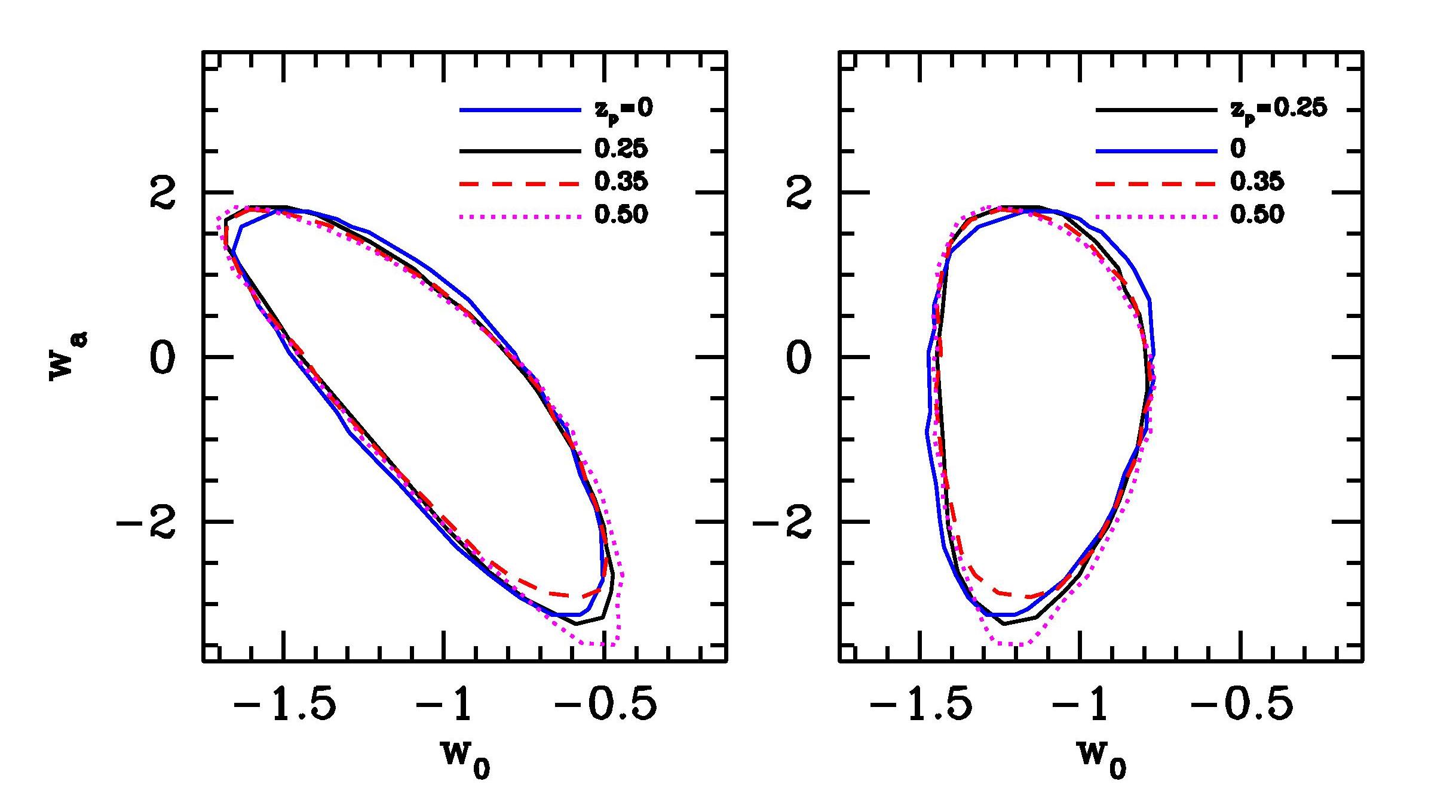
Let us then consider the fits when pivoting redshifts $z_{p}\neq 0$ are considered. In Figure 3 we overlap the 2$\sigma$ contour ellipses on the $w_{0}$–$w_{a}$ plane, for $z_{p}=0$, 0.25, 0.35 and 0.5, both for $f_{\nu}=0$ (l.h.s.) and $\neq 0$ (r.h.s.). For the sake of clarity, we consider only the full set of observational constraints (CMB+SN+BAO+HST). The ellipses exhibit a progressive straightening of the symmetry axes and $w_{0}$–$w_{a}$ errors become uncorrelated when $z_{p}\simeq 0.35$ or $z_{p}\simeq 0.25$, in the cases $f_{\nu}=0$ or $\neq 0$. More precisely, with the system of data used here, the covariance Cov$(w_{0},w_{a})=\langle(w_{0}-\bar{w}_{0})(w_{a}-\bar{w}_{a})\rangle$ vanishes for $z_{p}=0.33$ or $z_{p}=0.24$, respectively, as is shown by Figure 4. Here $\bar{w}_{0}$ and $\bar{w}_{a}$ are mean values at those redshifts.

Figure 3: 2$\sigma$ marginalized likelihood contours on the $w_{0}-w_{a}$ plane for different values of $z_{p}$, as indicated in the frame; $w_{0}$ and $w_{a}$ exhibit uncorrelated errors for $z_{p}\simeq 0.35$ (0.25) when $f_{\nu}\equiv 0$ ($\neq 0$). Notice the color and linetype inversion between $z_{p}=0.25$ and 0.35, in the two Figures. All plots refers to CMB+SN+BAO+HST constraint combination.

Figure 4: Dependence on $z_{p}$ of the $w_{0}$–$w_{a}$ covariance. This plot confirms that the two parameter estimates are statistically independent for $z_{p}\simeq 0.35~{}\,(0.25)$ if neglecting (allowing) neutrino mass. According to the plot, statistical independence occurs exactly at $z_{p}=0.33~{}\,(0.24)$, respectively. Data improvements might however cause small shift of these “exact” values.

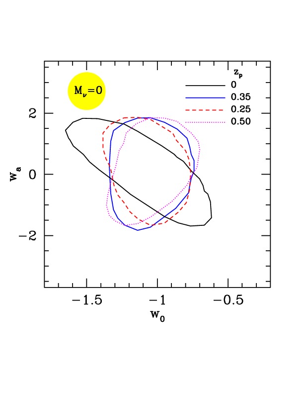
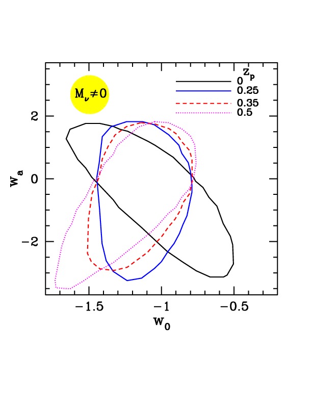
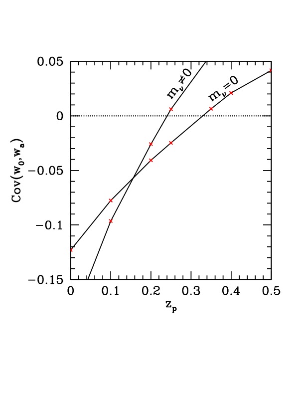
Such difference between the two cases is a result of this analysis. Notice again that the overall ellypsoïdal areas are much greater on the r.h.s. This is the effect of adding just one extra parameter and confirms that a significant correlation exists between the allowed $w_{0}$–$w_{a}$ domains and $M_{\nu}$, so that neglecting the $\nu$–mass option can be badly misleading, when we aim to constrain the DE state equation.

The ellipses in Figure 3 apparently undergo a gradual distortion and migrate through the plot. This is because each coefficient pair $w_{0}$–$w_{a}$ (i.e. $w_{0,a_{p}}$–$w_{a,a_{p}}$) corresponds to a different straight line, when $a_{p}$ varies.

It is however possible to translate the constraints found at any $a_{p}$ into constraints on the $w_{0,a_{p}=1}$–$w_{a,a_{p}=1}$ plane, or into constraints on the plane spanned by the coefficients $w_{0}$–$w_{a}$ when $z_{p}=0$, or when $z_{p}$ yields uncorrelated errors. In the Figures 5 we show the shapes of the ellipses after this transformation. The two Figures on the first (second) line refer to $f_{\nu}\equiv 0$ ($f_{\nu}\neq 0$). The Figures at the l.h.s. (r.h.s.) are the ellipses at $z=0$ ($z=0.35$ or 0.25 close to where parameter errors are uncorrelated).

Figure 5: 2$\sigma$ marginalized likelihood contours on the $w_{0}-w_{a}$ plane, obtained with different $z_{p}$ and translated to a unique redshift. All plots refers to CMB+SN+BAO+HST constraint combination. Plots at the l.h.s. (r.h.s.) are translated to $z=0$ (to the redshift where $w_{0}$ and $w_{a}$ constraints are uncorrelated). The 2 plots on the first (second) row are for $f_{\nu}\equiv 0$ ($f_{\nu}\neq 0).$

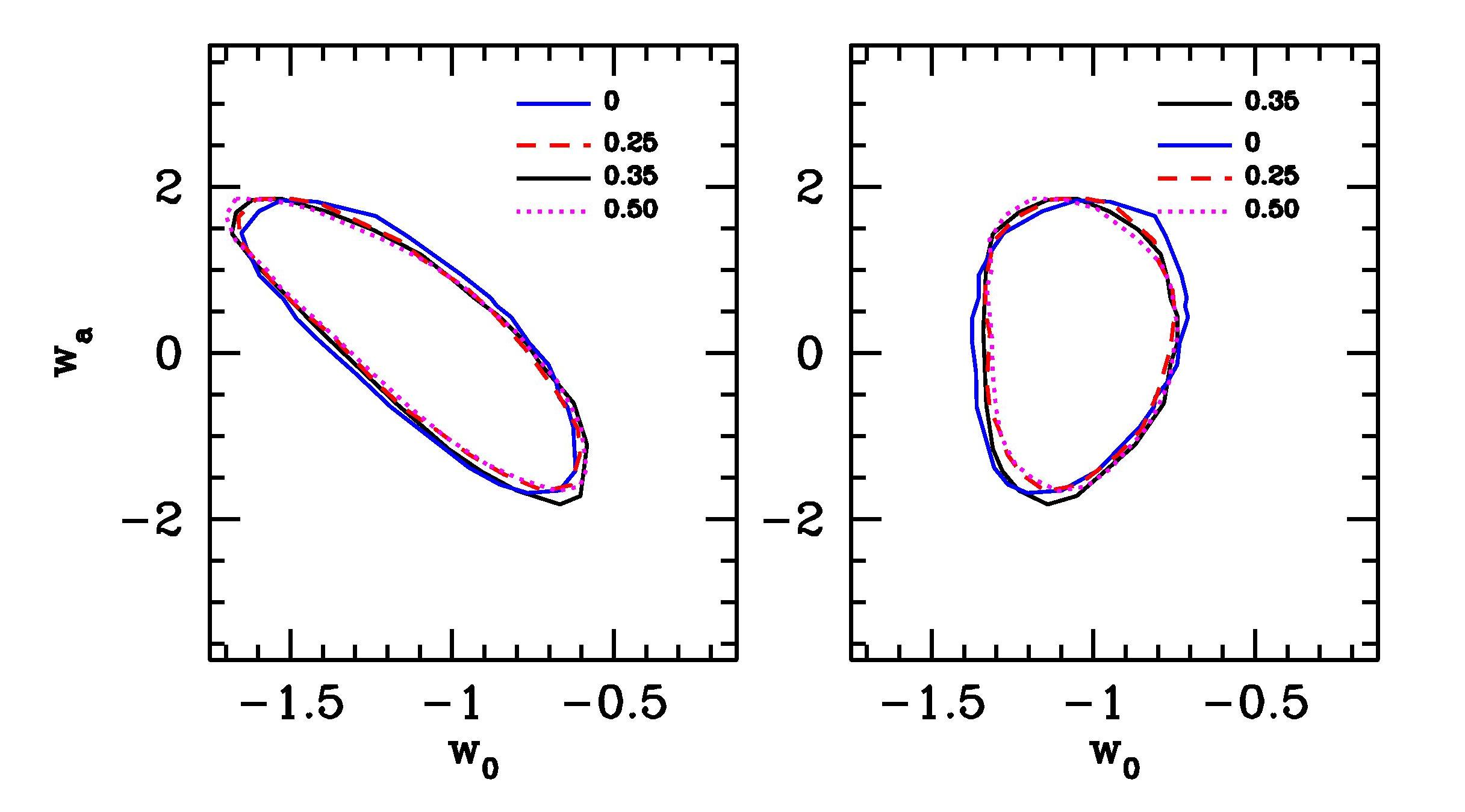
These plots are one of the results of this analysis. They confirm the high reliability of the MC algorithm, yielding close results when different parameter combinations are fitted.

Residual slight differences between the plotted ellipses are a measure of the reliability of the algorithm used.

	Massless	Neutrinos	Massive	Neutrinos
$z_{p}$	$w_{0}\pm 1\sigma\pm 2\sigma$	$w_{a}\pm 1\sigma\pm 2\sigma$	$w_{0}\pm 1\sigma\pm 2\sigma$	$w_{a}\pm 1\sigma\pm 2\sigma$	$f_{\nu}\pm 1\sigma\pm 2\sigma$
$0$	$-1.13_{-0.10-0.30}^{+0.09+0.33}$	$0.29_{-0.25-1.30}^{+0.39+1.00}$	$-1.07_{-0.11-0.34}^{+0.10+0.38}$	$-0.31_{-0.34-1.89}^{+0.56+1.37}$	$0.036_{-0.036-0.036}^{+0.009+0.041}$
$0.1$	$-1.11_{-0.07-0.22}^{+0.06+0.23}$	$0.32_{-0.24-1.29}^{+0.40+0.97}$	$-1.10_{-0.07-0.24}^{+0.07+0.24}$	$-0.27_{-0.36-1.78}^{+0.53+1.34}$	$0.035_{-0.035-0.035}^{+0.009+0.040}$
$0.2$	$-1.08_{-0.05-0.16}^{+0.05+0.16}$	$0.31_{-0.26-1.32}^{+0.40+1.03}$	$-1.12_{-0.05-0.18}^{+0.05+0.18}$	$-0.32_{-0.34-1.93}^{+0.58+1.36}$	$0.036_{-0.036-0.036}^{+0.010+0.041}$
$0.25$	$-1.07_{-0.04-0.14}^{+0.04+0.14}$	$0.32_{-0.23-1.27}^{+0.39+0.97}$	$-1.13_{-0.04-0.18}^{+0.05+0.16}$	$-0.28_{-0.36-1.95}^{+0.58+1.43}$	$0.035_{-0.035-0.035}^{+0.009+0.041}$
$0.35$	$-1.05_{-0.03-0.14}^{+0.04+0.13}$	$0.28_{-0.24-1.32}^{+0.39+0.99}$	$-1.14_{-0.04-0.22}^{+0.06+0.17}$	$-0.24_{-0.37-1.82}^{+0.55+1.36}$	$0.035_{-0.035-0.035}^{+0.010+0.040}$
$0.4$	$-1.05_{-0.03-0.15}^{+0.04+0.13}$	$0.29_{-0.24-1.33}^{+0.40+0.98}$	$-1.15_{-0.04-0.26}^{+0.08+0.19}$	$-0.30_{-0.36-1.86}^{+0.57+1.37}$	$0.036_{-0.036-0.036}^{+0.009+0.041}$
$0.5$	$-1.03_{-0.03-0.18}^{+0.05+0.13}$	$0.30_{-0.24-1.32}^{+0.40+0.96}$	$-1.17_{-0.05-0.34}^{+0.10+0.22}$	$-0.32_{-0.35-1.93}^{+0.57+0.40}$	$0.035_{-0.035-0.035}^{+0.010+0.040}$

Table 2: Mean and fully marginalized limits at $1\sigma$ and $2\sigma$ for different pivoting redshifts. In all the cases the data set is CMB+SN+BAO+HST.

Figure 6: On the l.h.s. (r.h.s) plot of mean, $1\sigma$ and $2\sigma$ limits on $w_{0}$ (mean and $1\sigma$ limits on $w_{a}$) at different $z_{p}$, for massless or massive neutrinos as indicated on the frame. In all cases, the constraint combination is (CMB+SN+BAO+HST).

4 Discussion

Linear DE state equations $w(a)$ are expressed by using $w_{0,a_{p}}$ and $w_{a,a_{p}}$ coefficients (usually $w_{0}$ and $w_{a}$) which do depend on the pivot $a_{p}$ value selected. Data yield constraints on $w_{0,a_{p}}$ and $w_{a,a_{p}}$ which turn out to be uncorrelated for a single $z_{p}$ value. We confirm that the pivoting redshift yielding no correlation is $\simeq 0.35$, if $f_{\nu}=0$, but we find that it lowers to $\sim 0.25$ if a degree of freedom allowing for the $\nu$–mass is open.

If we follow the procedure suggested by the Dark Energy Task Force (Albrecht et al. (2006)) to evaluate a Figure of Merit (FoM) for the precision of the two fits, we find

$$[\sigma(w_{a})\times\sigma(w_{0})]^{-1}=9.71~{}~{}{\rm or}~{}~{}17.2$$ (6)

in the $M_{\nu}\neq 0$ or $\equiv 0$ cases, respectively. The standard deviations $\sigma(w_{a})$ and $\sigma(w_{0})$ are evaluated at the $z_{p}$ value allowing independent $w_{a}$ and $w_{0}$ estimates, by fitting a Gaussian distribution on the posterior distribution. These values agree with DETF expectations, suggesting a range between 6.1 and 35.2. By using WMAP5, BAO and SN data, Wang (2008) found FoM=8.3 . By using just more recent BAO and SN constraints, Sendra & Lazkoz (2012) found FoM=14.2. Our slightly greater FoM arises from the improved and wider set of data. For the sake of comparison, still according to Salzano et al. (2012), when linear laws are parametrized by the values of $w$ at $z=0$ and 0.5, the FoM is $\sim 25~{}$.

Figure 7: Envelop of DE state equations (eq. 2). The plot is built by using $w_{0}$ and $w_{a}$ values with uncorrelated errors. Any straight line completely inside the black contours is an allowed DE state equation. Using other pivoting $z_{p}$ causes almost irrelevant changes (apart of the case $z_{p}=0$ with $f_{\nu}=0$). For the sake of comparison, the green dashed lines limit the $w_{0}$ interval allowed when we fit data by using varying $a_{p}$. The data set is (CMB+SN+BAO+HST).

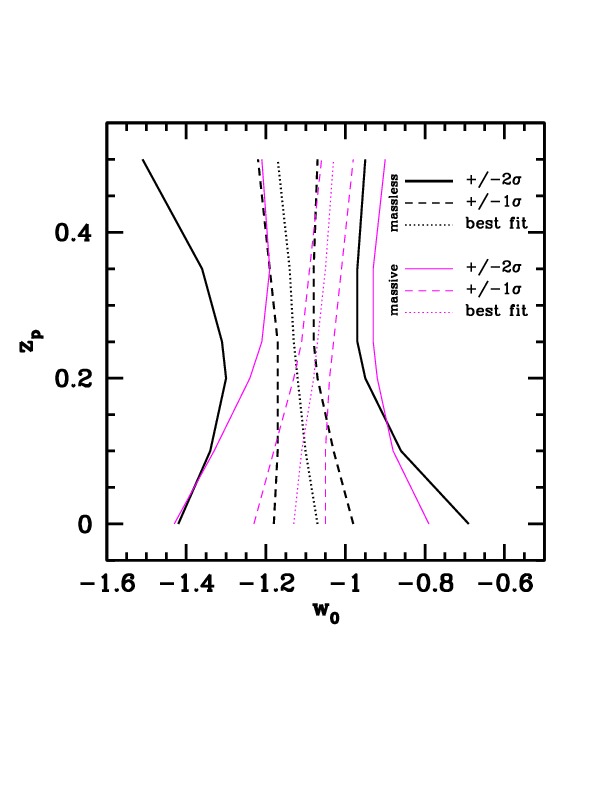
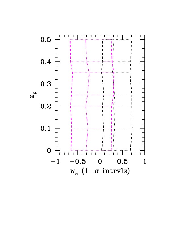
The $w_{0}$–$w_{a}$ ranges found in the cases $M_{\nu}\equiv 0$ and $M_{\nu}\neq 0$ exhibit significant overlaps, as expected. Our finding is that the allowed $w_{0}$ range, when marginalizing in respect to any other parameter, exhibits different trends in the two cases: the $w_{0}$ range tends to decrease (increase) when the option $f_{\nu}\neq 0$ is allowed (disregarded). As a consequence, the $w_{0}$ intervals show no overlap (at 1$\sigma$) when the pivot redshift exceeds $\sim 0.4$ (see Figure 6, l.h.s.). We also plot the $z_{p}$ dependence of $w_{a}$ 1$\sigma$ errorbars (Figure 6, r.h.s.), confirming $w_{a}$ estimates to be smaller when $M_{\nu}\neq 0$ is allowed. Clearly, no $z_{p}$ dependence is evident here. For more details results see Table 2.

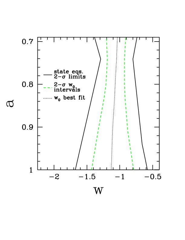
The set of linear $w(a)$ laws should however be independent of the pivoting redshift. In Figure 7 we show the line envelops for the cases $f_{\nu}=0$ (l.h.s.) and $\neq 0$ (r.h.s.). In the same plots we report also the $w_{0}$ constraints shown in the previous Figure, and the best fit $w_{0}$ at any redshift. A hint of the trends found in the evolution of the $w_{0}$ range (and $w_{0}$ best–fit value) can be seen also in the average behaviors of the fitting linear laws.

The fact that the linear laws are the same, independently of the $z_{p}$ chosen to perform the fit, is confirmed in Figures 5. The plots confirm the good performance of the MC algorithm, yielding overlapping results for different linear combinations of the fitting parameters.

5 WMAP9 release

After the completion of this work, nine–year WMAP data have been released, together with a number of fits on cosmological parameters (Hinshaw et al. (2012)).

We had mentioned that our curves are displaced towards significantly more negative $w_{0}$ and greater $w_{a}$ values, in respect to WMAP7 output analysis by Komatsu et al. (2011). WMAP9 ellipses fully confirm such displacement.

The main difference between ours and WMAP9’s results concerns the shape of the error distributions. Our peak about top likelihood values appears more pronounced, with an error distribution becoming much flatter above $\sim 1\sigma$. In fact, our 1$\sigma$ errors apparently yield even tighter constraints than WMAP9: the $w_{0}$/$w_{a}$ intervals pass from -1.23,-1.04/0.04,0.68 (our values) to -1.29,-1.04/-0.14,0.85 (WMAP9). The $w_{0}$ output are therefore overlappable, while also $w_{a}$ is equally centered, with an error drastically reduced from 0.99 to 0.64 .

The situation is clearly opposite if we consider the $w_{0}$ and $w_{a}$ intervals spanned by the 2$\sigma$ ellipse on the $w_{0}$–$w_{a}$ plane. By comparing Figure 10 in WMAP9 release with our Figure 1, we see intervals passing from -1.51,-0.84/-1.12,1.41 to -1.59,-0.61/-1.70,1.79 for $w_{0}$ and $w_{a}$, respectively.

The more pronounced Gaussian behavior in WMAP9 data is probably related to their greater dataset, also implying an enhanced disagreement for central and 1$\sigma$ values, but overall tighter constraints.