A variational approach to modeling slow processes in stochastic dynamical systems
Abstract.
The slow processes of metastable stochastic dynamical systems are difficult to access by direct numerical simulation due the sampling problem. Here, we suggest an approach for modeling the slow parts of Markov processes by approximating the dominant eigenfunctions and eigenvalues of the propagator. To this end, a variational principle is derived that is based on the maximization of a Rayleigh coefficient. It is shown that this Rayleigh coefficient can be estimated from statistical observables that can be obtained from short distributed simulations starting from different parts of state space. The approach forms a basis for the development of adaptive and efficient computational algorithms for simulating and analyzing metastable Markov processes while avoiding the sampling problem. Since any stochastic process with finite memory can be transformed into a Markov process, the approach is applicable to a wide range of processes relevant for modeling complex real-world phenomena.
1. Introduction
In this article, we consider continuous-time Markov processes living in a usually large state space that is either continuous or discrete. The process is considered to be sufficiently ergodic such that a unique stationary density (invariant measure) exists. Independent of the details of the dynamics (such as system size, potential, stochastic coupling, etc), there exists a family of linear propagators which evolve the probability density of states as:
| (1.1) |
Continuous-time Markov processes are useful models of real-world processes in a variety of areas [44]. Examples include macroscopic phenomena including the evolution of financial and climate systems [24, 30], as well as microscopic dynamics such as the diffusion of cells in liquids [1], the diffusion of biomolecules within cells [41], the stochastic reaction dynamics of chemicals at surfaces [31], and the stochastic dynamics governing the structural dynamics of molecules [2]. Often, these dynamics are metastable, i.e. they consist of slow processes between sets of state space that have long lifetimes. In macromolecules, such slowly-exchanging sets are called conformations, hence the union of the slowest dynamical processes are there termed conformation dynamics [35, 37].
In practice, the slow dynamical processes are the ones which pose the greatest difficulties to direct numerical simulation as they require the longest simulation times. An extreme example is the atomistic simulation of solvated biomolecules which would require the propagation of a system with particles for time-steps, a task that is intractable or hardly tractable even with special-purpose supercomputers [39]. However, the slowest processes are also the ones that are the most interesting in many systems. They often correspond to rare events that change the global structure and/or the functional behavior of the system. For example, in macromolecular systems, the slowest events often correspond to functional conformational changes such as folding, binding or catalysis [28, 45, 7, 21]. Therefore, a method is sought that models the slow dynamical processes of continuous-time Markov processes accurately and ideally in a way that supports the efficient simulation of these processes without the need to solve the full direct numerical simulation problem.
Especially in statistical physics, many theories and methods have been proposed to model slow dynamical processes. Examples are rate theories that describe the passage rate of a process across a surface that separates metastable states [15, 20], pathway-based theories and methods that describe the transition dynamics of a system from a subset to a subset of state space [14, 3, 25] and network-based approaches that attempt to coarse-grain the high-dimensional dynamics to a network of discrete jump events between sub-states or landmarks [47, 48]. These approaches usually assume a separation of timescales between the slow and the fast processes that results from vanishing smallness parameters (e.g. noise intensity, temperature). In these cases, the mathematical analysis can be based on large deviation estimates and variational principles [16, 14].
In this article, we consider a more general approach to describing slow dynamical processes. When the operator is compact and self-adjoint, eq. (1.1) can be decomposed into the propagator’s spectral components
| (1.2) |
where are the propagator’s eigenfunctions and (sorted in non-ascending order) are the propagator’s real-valued eigenvalues that decay exponentially in time with rates . are factors depending on the initial density . We here consider the situation that the eigenspaces of slow and fast processes are orthogonal. For example, in the important case that the system studied is a microscopic physical system in thermal equilibrium, such that the process is reversible with respect to the invariant density , the eigenspaces of slow and fast processes are orthogonal for any choice of . In such a case, is a model parameter that can be chosen to distinguish the slow processes of interest from the fast processes that are not of interest. For initial densities , the term for fast processes in Eq. (1.2) vanishes and the propagation can be performed exactly using only the dominant eigenfunctions. Note that Eq. (1.2) represents the formulation of the dynamical process problem as a multi-scale problem in time: represents the timescale , is the slowest dynamical process, etc. This formulation thus allows essential characteristics of the dynamical process to be described by treating its scales separately. The relation between dominant eigenvalues, exit times and rates, and metastable sets has been studied by asymptotic expansions in certain smallness parameters as well as by functional analytic means without any relation to smallness parameters [23, 12, 46, 4, 5]. In particular, [10, 11] established fundamental relations between the eigenvalues and -functions of and metastable sets.
The task is now to approximate the propagator’s dominant eigenfunctions and eigenvalues . In other disciplines, variational principles have been worked out in order to approximate eigenfunctions and eigenvalues of known operators such as a quantum-mechanical Hamiltonian [43]. In contrast, for many complex dynamical systems, is either not known explicitly, or not available in a form that can be transformed into Eq. (1.2). Instead, is given implicitly through stochastic realizations of the process . Therefore, a variational principle is sought that allows eigenfunctions and eigenvalues to be approximated through statistical observables of . Such a variational principle will be formulated in the present paper.
This problem has extensively been studied for specific functional forms of the eigenfunctions . When are approximated via characteristic functions on a given set decomposition of state space, i.e. with , the problem of finding the best approximation to eigenfunctions and eigenvalues is solved by a Markov model or Markov state model (MSM) [35, 4, 12, 34, 27, 22]. In another version of MSMs, are approximated by committor functions between a few pre-defined “cores” that form a non-complete subset of state space [8, 13, 36]. Basis functions that form a partition of unity are used in [49]. Markov state models have been recently used a lot to model molecular dynamics processes, especially in conjunction with large amounts of distributedly simulated trajectories [42, 40, 9, 26, 8, 28]. Applications include conformational rearrangements and folding of peptides, proteins and RNA [9, 29, 6, 28, 45, 27]. In this application area, MSMs have had significant impact because they can be estimated from relatively short simulation trajectories and yet allow the system behavior to be predicted at long timescales.
Despite this success, significant challenges remain. For example, in most current applications, the discretization of state space is done heuristically via a Voronoi partition of state space obtained from clustering available data points. The ability to construct a state space discretization adaptively would tremendously aid the construction of MSMs that are precise while avoiding the use of too many states. Such an adaptive discretization must be guided by an objective function that somehow measures the error made by the model. A bound to the MSM discretization error has been derived in [34]. However, this error is not suitable to design a constructive discretization approach as its evaluation requires knowledge of the exact eigenfunctions. The variational principle derived in this paper only uses statistical observables and is henceforth the basis for such a constructive approach to adaptive discretization. Furthermore, it is shown that existing Markov modeling approaches can be understood as a constrained optimal solution of the variational principle via a Ritz or Roothan-Hall method with different choices of basis sets. Based upon this formulation, further development of basis sets appropriate for describing complex molecular conformation dynamics can be made.
The article is organized as follows: In Sec. 2 a variational principle is formulated where the dominant eigenfunctions of stochastic dynamical systems are approximated by maximizing a Rayleigh coefficient, which - in the limit of the exact solution - is identical to the true eigenvalues. This Rayleigh coefficient is linked to the computation of correlation functions that can be evaluated without explicit knowledge of the propagator . Sec. 3 makes considerations which types of functions may be practically useful to construct an approximation to Eq. (1.2) in complex systems. Sec. 4 shows numerical experiments on a diffusion process in a one-dimensional double-well potential. Sec. 5 concludes this study and makes suggestions for the next steps
2. Variational principle for conformation dynamics
2.1. Basics
Let be a state space, and let us use to denote points in this state space. We consider a Markov process on which is stationary and ergodic with respect to its unique stationary (invariant) distribution . The dynamics of the process are characterized by the transition density
| (2.1) |
which we assume to be independent of the time . The correlation density, i.e., the probability density of finding the process at points and at a time spacing of , is then defined by
| (2.2) |
We further assume to be reversible with respect to its stationary distribution, i.e.:
| (2.3) | |||||
| (2.4) |
Reversibility is not strictly necessary but tremendously simplifies the forthcoming expressions and their interpretation [34]. In physical simulations, reversibility is the consequence of the simulation system being in thermal equilibrium with its environment, i.e. the dynamics in the system is purely a consequence of thermal fluctuations and there are no external driving forces.
If, at time , the process is distributed according to a probability distribution , the corresponding distribution at time is given by:
| (2.5) |
The time evolution of probability densities can be seen as the action of a linear operator , called the propagator of the process. This is a well-defined operator on the Hilbert space of functions which are square-integrable with respect to the weight function . The scalar-product on this space is given by
| (2.6) |
If we assume the transition density to be a smooth and bounded function of and , the propagator can be shown to be bounded, with operator norm less or equal to one. Since the stationarity of implies , we even have . Reversibility allows us to show that the propagator is self-adjoint and compact. Furthermore, using the definition of the transition density, we can show that satisfies a Chapman-Kolmogorov equation: For times , we have
| (2.7) |
2.2. Spectral decomposition
It follows from the above arguments that possesses a sequence of real eigenvalues , with and . Each of these eigenvalues corresponds to an eigenfunction . The functions form an orthonormal basis of the Hilbert space . Clearly, is an eigenvalue with eigenfunction . In many applications, we can assume that is non-degenerate and is not an eigenvalue. Additionally, there usually is a number of positive eigenvalues
| (2.8) |
which are separated from the remaining spectrum. Because of the Chapman-Kolmogorov equation, each eigenvalue decays exponentially in time, i.e. we have
| (2.9) |
for some rate . Clearly, , are close to zero, and all remaining rates are significantly larger than zero. If we now expand a function in terms of the functions , i.e.
| (2.10) |
we can decompose the action of the operator into its action on each of the basis functions:
| (2.11) |
For lag times , all except the first terms in the above sum have become very small [34], and to a good approximation we have
| (2.12) |
Knowledge of the dominant eigenfunctions and eigenvalues is therefore most helpful to the understanding of the process.
Remark 1.
Instead of the propagator , one can also consider the transfer operator , defined for functions by:
| (2.13) |
Using the unitary multiplication operator , defined by
| (2.14) |
we have
| (2.15) |
and consequently, the transfer operator inherits all of the above properties from . In particular, there is a sequence of eigenfunctions
| (2.16) |
of , corresponding to the same eigenvalues , which are normalized w.r.t. to the scalar-product weighted with instead of . Especially, we have =1 . The two operators can be treated as equivalent, and all of the above could have been formulated in terms of as well.
2.3. Rayleigh variational principle
In nontrivial dynamical systems neither the correlation densities and nor the eigenvalues and eigenfunctions are analytically available. This section provides a variational principle based on which these quantities can be estimated from simulation data generated by the dynamical process . For this, the formalism introduced above is used to formulate the Rayleigh variational principle used in quantum mechanics [43] for Markov processes.
Let be a real-valued function of state, . Its autocorrelation with respect to the stochastic process is given by:
| (2.17) |
In the Dirac notation often used in physical literature, integrals such as the one above may be abbreviated by .
Theorem 2.
The autocorrelation function of a weighted eigenfunction is its eigenvalue :
| (2.18) |
Theorem 3.
Let be an approximate model for the second eigenfunction, which is normalized and orthogonal to the true first eigenfunction:
| (2.20) | |||||
| (2.21) |
Then we find for :
| (2.22) |
Proof.
The proof is an application of the Rayleigh variational method to the operator . If is written in terms of the basis of eigenfunctions :
| (2.23) |
where because of the orthogonality condition, we find:
| (2.24) |
The pre-last estimate is due to the ordering of the eigenvalues, and the last equality results from the normalization condition 2.21 and Parseval’s identity.∎
Corollary 4.
Similarly, let be an approximate model for the ’th eigenfunction, with the normalization and orthogonality constraints:
| (2.25) | |||||
Remark 5.
Improved estimates than those of 2 to 4 have been obtained by [22] for characteristic functions. With a re-definition of the terminology, they can be directly transferred to the case of mutually orthonormal basis functions. It would be interesting to study the applicability of these results to more general cases. However, obtaining such estimates is not the focus of the present paper.
Remark 6.
The variational principle given by Theorems (2) to (4) is fulfilled for with only if the dominant eigenfunctions are already known.
In particular, the first eigenfunction, i.e. the stationary density must be known. In practice, these eigenfunctions are approximated via solving a variational principle. Nonetheless, some basic statements can be made even if no eigenfunction is known exactly. For example, it is trivial that when the estimated stationary density is used in Theorem 2, then the estimate of the first eigenvalue is still always correctly 1:
| (2.27) |
and from theorems 2 and 3 it follows that any function
| (2.28) |
hence the eigenvalue 1 is simple and dominant also when estimating eigenvalues from data.
Remark 7.
An important insight at this point is that a variational principle of conformation dynamics can be formulated in terms of correlation functions. In contrast to quantum mechanics or other fields where the variational principle has been successfully employed, no closed-form expression of the operator is needed. The ability to express the variational principle in terms of correlation functions with respect to means that the eigenvalues to be maximized can be directly estimated from simulation data. If statistically sufficient realizations of are available, then the autocorrelation function can be estimated via:
| (2.29) |
where is the number of simulated time windows of length . We will try to use this in the application of the method.
2.4. Ritz method
The Ritz method is a systematic approach to find the best possible approximation to the first eigenfunctions of an operator simultaneously in terms of a linear combination of orthonormal functions [32]. Here the Ritz method is simply restated in terms of the present notation. Let , be a set of orthonormal basis functions:
| (2.30) |
and let denote the vector of these functions:
| (2.31) |
We seek a coefficient matrix ,
| (2.32) |
with the column vectors that approximate the eigenfunctions of the propagator as:
| (2.33) |
with respect to the constraint that the functions are also normalized. It turns out that the solution to the eigenvalue equation
| (2.34) |
with individual eigenvalue/eigenvector pairs
| (2.35) |
and the density matrix defined by:
| (2.36) | |||||
| (2.37) |
yields the desired result. More precisely, the eigenvector corresponding to the greatest eigenvalue from 2.35 contains the coefficients of the linear combination which maximizes the Rayleigh coefficient among the functions , and this maximum is given by Consequently, should be as close as possible to , and the function generated from should model the stationary density . But furthermore, the remaining eigenvalues and eigenvectors generated from (2.34) can be used as estimates of the other eigenvalues :
Corollary 8.
The second estimated eigenvalue from (2.35) satisfies .
Proof.
First of all, note that by the orthogonality of the eigenvectors of the matrix . For the same reason, we find that:
| (2.38) | |||||
Now, let be a linear combination of the first two model eigenfunctions which is normalized such that
| (2.39) | |||||
| (2.40) | |||||
which is bounded from below by . Clearly, there is a normalized linear combination of and which is orthogonal to . By (2.40) and the variational principle, we conclude that:
∎
2.5. Roothaan-Hall method
The Roothaan-Hall method is a generalization of the Ritz method used for solving the linear parameter optimization problem for the case when the basis set is not orthogonal [33, 19]. Let the matrix with elements
| (2.41) |
be the matrix of overlap integrals with the normalization conditions . Note that has full rank if and only if all are pairwise linearly independent. The optimal solutions in the sense of Eqs (2.32)-(2.33) are found by the eigenvectors of the generalized eigenvalue problem:
| (2.42) |
with the individual eigenvalue/eigenvector pairs:
| (2.43) |
Remark 10.
The Ritz and Roothaan-Hall methods are useful for eigenfunction models that are expressed in terms linear combinations of basis functions. Non-linear parameter models can also be handled with nonlinear optimization methods. In such nonlinear cases it needs to be tested whether there is a unique optimum or not.
2.6. Markov state model
As an example, let be pairwise disjoint sets partitioning and let be the stationary probability of set . Consider the piecewise constant functions
| (2.44) |
where is the characteristic function that is 1 for and 0 elsewhere. Since for all these functions form a basis set with . Therefore, we can directly use them as a model for the transfer operator eigenfunctions . Evaluation of the corresponding matrix yields:
where is the joint probability of observing the process in sets and with a time lag of while is the corresponding transition probability. Thus, computing the optimal step-function approximation to the true eigenfunctions and eigenvalues via the Ritz method is the same as computing eigenvalues and eigenvectors of the Markov model transition matrix and scaling them appropriately. This conclusion can also be obtained from Ref. [34] via a different route.
3. Modeling
Section 2 has provided a general variational principle for approximating the dominant eigenvalues and eigenfunctions of Markov processes. In order to apply this principle to complex systems, a useful level of modeling the eigenfunctions in terms of basis functions needs to be found, and appropriate classes of basis functions must be identified. This sections attempt a first approach to this problem by making general considerations for what modeling schemes might be appropriate.
3.1. Half-weighted eigenfunctions
Is it beneficial to directly model the propagator eigenfunctions , their weighted counterparts or rather yet another set of functions? We would like to use a model that has the following properties:
-
(1)
As basis functions it is preferred to use local functions, i.e. either functions with compact support, or at least with the property . Such locality is useful to direct the computation effort to specific regions of state space and may aid the adaptive refinement of the eigenfunction approximation by specifically adding basis functions that add local refinements. Since we also aim at modeling eigenfunctions as linear combinations of basis functions we cannot use the eigenfunctions that are not local.
-
(2)
We would like to be able to pre-compute as many expressions as possible analytically. When using appropriate basis functions and it may be possible to calculate analytic solutions of the integrals , albeit this feature is usually destroyed when weighting with the stationary density as in . Therefore we will also avoid using the eigenfunctions that would require such a weighting.
Consider a rewrite of Eq. (2.17) as:
| (3.1) | |||||
where the “half-weighted” eigenfunctions:
| (3.2) |
and the “half-weighted” correlation density:
| (3.3) |
have been defined. When now modeling the half-weighted eigenfunctions using some basis set, the following nice properties are obtained:
-
(1)
Local basis functions can be used. This follows from
-
(2)
The normalization condition requires a non-weighted scalar product:
-
(3)
When is analytically computable and , then is also analytically computable.
-
(4)
The first half-weighted eigenfunction has eigenvalue 1 and is identical to the half-weighted stationary density
(3.5) -
(5)
When models of and are available, the Rayleigh coefficient in Eq. (3.1) can be estimated numerically as the autocorrelation of
-
(6)
When defining a propagator in half-weighted space via:
(3.6) then is self-adjoint and has orthogonal eigenfunctions
(3.7)
It follows from theorem (2) that the exact eigenvalues are calculated by the Rayleigh coefficients of the exact eigenfunctions:
| (3.8) |
while they are approximated from below by the Rayleigh coefficients of the approximate eigenfunctions:
| (3.9) |
This Rayleigh-coefficient can be directly sampled: for a given trajectory , it can be estimated as:
| (3.10) |
Thus, for a given trajectory , the optimal eigenfunctions can be calculated by maximizing the Rayleigh coefficient, using e.g. the Ritz or the Roothaan-Hall method.
3.2. Gaussian Basis functions
In complex dynamical processes such as molecular dynamics of biomolecules, one has to devise basis sets that can be evaluated in high dimensions. While the present work provides merely a starting point for identifying appropriate basis sets that go beyond common choices such as the step function basis or the committor basis, we here suggest a possible choice that is potentially applicable to the molecular dynamics setting. Empirically, it has been found that the stationary densities of biomolecules in the essential subspace is often clustered [18]. Therefore, we put forward the idea that and the other half-weighted eigenfunctions can be approximated by a Gaussian mixture.
Let us thus assume that the state space is a metric space with distance , and let us model the half-weighted invariant density in terms of Gaussian basis functions:
| (3.11) |
where , and are amplitude, mean and shape parameters. The invariant density can then be analytically given:
Furthermore, consider that the half-weighted eigenfunctions be given in terms of the same Gaussian basis:
| (3.13) |
where must be appropriately chosen to guarantee orthogonality with respect to the invariant density. The corresponding unweighted eigenfunctions are
| (3.14) |
which does not have a simple form, but can be evaluated point-wise. In order to enforce the normalization we consider
| (3.15) |
which can be analytically evaluated when is an Euclidean space.
Using Gaussian Ansatz functions in half-weighted space may thus have important practical benefits. However, other basis sets, especially sets of other Radial basis functions than Gaussians may also be a good choice for high-dimensional systems that deserve further investigation.
4. Numerical examples
4.1. Metastable potential from a Gaussian stationary density
The example is chosen such that it is tractable by direct grid discretization so as to be able to generate a reference solution. Different optimization methods for the variational problem and choices of basis sets are considered and illustrated.
Let be our state space with points . First, a “Gaussian hat” function is defined via:
| (4.1) |
where is the mean and the standard deviation. We define a stationary density from two Gaussians:
The corresponding dimensionless generating potential is given by
| (4.2) |
which exerts a force on a particle at position of:
| (4.3) |
Using Smoluchowski dynamics and Euler discretization, a time-step is given by
| (4.4) |
where is a normally distributed random variable (white noise). The transition density can hence be written as:
| (4.5) |
and the correlation density is given by:
| (4.6) |
Now we are concerned about estimation of eigenfunctions. The first half-weighted eigenfunction is the square root of the stationary density:
| (4.7) |
such that . We here assume to be known, although in practice it must be estimated.
(a)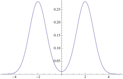 (b)
(b)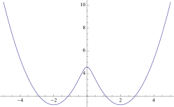
(c)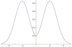 (d)
(d)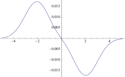
4.2. Ritz method with characteristic functions (Markov state model)
We aim at approximating the eigenvalues and eigenfunctions of the true propagator via the Ritz method described in Sec. 2.4. Here, a basis set consisting of 20 characteristic functions in the range defined by:
| (4.8) |
where is the characteristic function that is 1 on the interval and 0 outside, and is the stationary probability of the set . The corresponding density-matrix defined by (Dirac notation):
| (4.9) |
The matrix was calculated by direct numerical integration using Mathematica and the eigenvalue problem was subsequently solved, yielding the optimal coefficient vectors and that provide the approximations , and , . The results are given in Fig. 4.2 a and b, indicating that the eigenvalues are approximated to two significant digits while the eigenfunctions retain a significant discretization error that arises from the step-function basis used.
a)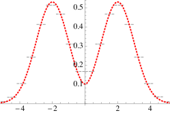 b)
b)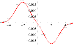
c)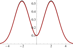 d)
d)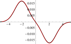
e)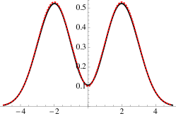 f)
f)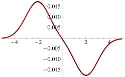
4.3. Ritz method with a Hermite basis
In order to arrive at a smooth solution we employ the Ritz method with a smooth orthogonal function basis. Here, we choose the Hermite functions, defined by:
| (4.11) |
The Hermite functions are local () and are thus useful to model the behavior of the eigenfunctions where the stationary density is significantly larger than zero. The basis functions are defined to be the normalized Hermite functions with
| (4.12) |
such that .
Using the basis set , the matrix was calculated by direct numerical integration using Mathematica and the Ritz method was used to approximate eigenvalues and eigenfunctions of the propagator. As shown in Fig. 4.2c and d, a nearly perfect approximation of both eigenvalues and eigenfunctions is obtained even though the number of basis functions used is identical to the MSM approach of the previous section. However, the MSM approach has the advantage that it can be employed in high-dimensional spaces which is not the case with Hermite basis functions.
4.4. Roothaan-Hall method with a Gaussian basis
In order to have a hope to solve high-dimensional problems, one must resort to simple basis functions, ideally ones with analytical properties that can be practically evaluated in high-dimensional spaces. Therefore, we here suggest the use of Gaussian basis functions as described in Sec. 3.2. In the one-dimensional case, the Gaussians used are:
| (4.13) |
Here, we use and . Gaussian basis functions are not orthogonal. We therefore calculate the overlap matrix with
that can be evaluated analytically. The matrix is again defined by (Dirac notation):
| (4.15) |
Using the Roothaan-Hall method (Sec. 2.5), the best approximation to the propagator eigenfunctions are found by the eigenvectors of the generalized eigenvalue problem
| (4.16) |
As shown in Fig. 4.2 c and d, an also nearly perfect approximation of both eigenvalues and eigenfunctions is achieved even though the basis is smaller than the previous basis sets. Since the Gaussian basis set is a good candidate for being used in high-dimensional spaces, this is probably the most useful result so far. Note that the matrix inversion can be efficiently calculated with sparse matrix methods when a cutoff is used to set nearly-non-overlapping pairs with to 0.
4.5. Nonlinear optimization
The previous methods used exclusively linear combinations of basis functions. A greater degree of freedom in approximating the propagator eigenfunctions is achieved by using additional shape parameters in the basis functions. This, however, leads to a nonlinear optimization problem that is in general difficult to solve and may have multiple optima. However, we briefly illustrate the approach on our one-dimensional example. We make the Ansatz for the second half-weighted eigenfunction:
| (4.17) | |||||
The normalization constant makes sure that . The constraint is here ensured by the fact that is an even function and is an odd function.
The optimal parameters and are found by maximizing the Rayleigh coefficient:
| (4.18) |
Fig. 4.3 shows the results of varying and as well as the local optimum for and . In this case, a good approximation to the eigenvector could be achieved with a 2-term ansatz function. However, the general usefulness of the nonlinear approach for high-dimensional problems remains to be evaluated.
(a)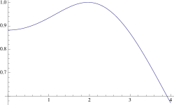 (b)
(b)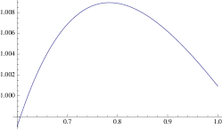 (c)
(c)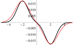
4.6. Quartic potential
As a second numerical example, we use the diffusion in a one-dimensional quartic potential:
| (4.19) |
which has two minimum positions at . We seek to estimate the second dominant eigenvalue and the corresponding time scale by applying the Roothaan-Hall method above with Gaussian functions. We will then compare the results to those obtained from a Markov state model discretization. First, we generate a sample trajectory of the process as in Eq. (4.4). Here, we used a time step and a total number of steps . From this sample, we computed an estimate of the stationary density. We then computed the Markov state model transition matrix and its eigenvalues, using a discretization of the state space into sets.
For the application of the Roothaan-Hall method, we picked thirteen Gaussian functions with centres at
| (4.20) |
The variances were set to for the functions centred at , and to for all others. Those functions were used as half-weighted basis functions, meaning that we computed the entries of the -matrix according to
| (4.21) |
where is an integer corresponding to the lag time . We similarly estimated the -matrix and then solved the generalized eigenvalue problem Eq. (2.42).
a)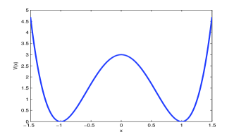 b)
b)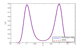
c)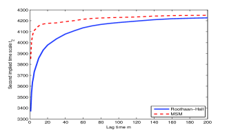 d)
d)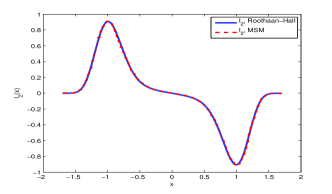
The results displayed in Figure 4.4 show that we not only get a good approximation of both the first and second eigenfunction in terms of smooth functions, but most importantly, the second largest eigenvalue and the corresponding time scale can be estimated comparably well with both methods. While sets were used for the MSM discretization, only thirteen basis function were used for the Roothaan-Hall method.
5. Conclusions and outlook
Here, we have formulated a variational principle for Markov processes where the dominant eigenfunctions are approximated by maximizing a Rayleigh coefficient, which - in the limit of the exact eigenfunctions - is identical to the true eigenvalues. This is the formulation needed to attack the problem of estimating the slow processes in stochastic dynamical systems with a much wider methodology than by the presently used class of Markov State Models. In particular, the entire toolbox of quantum mechanics where many decades of research have gone into the development of eigenfunction approximation methods for high-dimensional systems becomes available.
From a practical point of view, a main achievement of the present study is that the Rayleigh coefficient can be estimated from simulation data as it is equivalent to an autocorrelation function of the appropriately weighted test function. The autocorrelation estimates are such that they can be fed by many short simulations distributed across state space and do not require the direct simulation of the slow processes in a single long trajectory. This is an important advantage in dealing with the sampling problem that arises in simulating metastable dynamical systems.
A main use of the present approach will be to facilitate the development of adaptive discretization algorithms of high-dimensional state spaces for the computational characterization of complex dynamical processes. The Rayleigh coefficient derived here represents a practically accessible and theoretically solid functional to guide such an adaptive discretization algorithm. In contrast to Markov state models, such an approximation approach does not necessarily need to use the same basis set for all eigenfunctions. Especially for reversible dynamics, different eigenfunctions can be approximated separately, thus possibly permitting the use of relatively small basis sets.
For a given class of dynamical systems, a basis sets must be selected that is appropriate to model the regularity of the solution. For high-dimensional processes such as molecular dynamics, Gaussian basis functions might be a workable solution since they be well combined with clustering-based identification of center positions and permit the analytical calculation of some quantities such as the overlap integral. An interesting alternative approach is to build the Basis set upon weakly coupled subsets of internal molecular coordinates, as suggested in the mean field approach developed in Ref. [17]. The usefulness of these and other approaches for complex molecular systems will be investigated in future studies. Furthermore, subsequent studies will deal with the error caused by the projection on a finite-dimensional subspace depending on the choice of basis functions, as well as with statistical considerations, such as the efficient evaluation of uncertainties of the estimated Rayleigh coefficients.
Acknowledgements
We gratefully acknowledge the DFG research center Matheon and the Berlin Mathematical School (BMS) for funding. We would also like to thank a number of colleagues for stimulating discussions, in particular: Christof Schütte, Guillermo Perez-Hernandez, Bettina Keller, Jan-Hendrik Prinz, Benjamin Trendelkamp-Schroer (all FU Berlin), and John D. Chodera (UC Berkeley).
References
- [1] K. Anguige and C. Schmeiser. A one-dimensional model of cell diffusion and aggregation, incorporating volume filling and cell-to-cell adhesion. Journal of mathematical biology, 58(3):395–427, March 2009.
- [2] Robert B. Best and Gerhard Hummer. Coordinate-dependent diffusion in protein folding. Proc. Natl. Acad. Sci. USA, 107(3):1088–1093, January 2010.
- [3] Peter G. Bolhuis, David Chandler, Christoph Dellago, and Phillip L. Geissler. Transition path sampling: throwing ropes over rough mountain passes, in the dark. Annu. Rev. Phys. Chem., 53(1):291–318, 2002.
- [4] A. Bovier, M. Eckhoff, V. Gayrard, and M. Klein. Metastability in reversible diffusion processes. i. sharp asymptotics for capacities and exit times. J. Eur. Math. Soc., 6:399424, 2004.
- [5] A. Bovier, M. Eckhoff, V. Gayrard, and M. Klein. Metastability in reversible diffusion processes. i. precise asymptotics for small eigenvalues. J. Eur. Math. Soc., 7:6999, 2005.
- [6] Gregory R. Bowman, Kyle A. Beauchamp, George Boxer, and Vijay S. Pande. Progress and challenges in the automated construction of Markov state models for full protein systems. J. Chem. Phys., 131(12):124101+, September 2009.
- [7] Gregory R. Bowman, Vincent A. Voelz, and Vijay S. Pande. Atomistic Folding Simulations of the Five-Helix Bundle Protein Lambda 6-85. Journal of the American Chemical Society, 133(4):664–667, February 2011.
- [8] Nicaolae V. Buchete and Gerhard Hummer. Coarse Master Equations for Peptide Folding Dynamics. J. Phys. Chem. B, 112:6057–6069, 2008.
- [9] J. D. Chodera, K. A. Dill, N. Singhal, V. S. Pande, W. C. Swope, and J. W. Pitera. Automatic discovery of metastable states for the construction of Markov models of macromolecular conformational dynamics. J. Chem. Phys., 126:155101, 2007.
- [10] E. B. Davies. Metastable states of symmetric markov semigroups i. Proc. London Math. Soc., 45:133–150, 1982.
- [11] E. B. Davies. Metastable states of symmetric markov semigroups ii. J. London Math. Soc., 26:541–556, 1982.
- [12] P. Deulfhard, W. Huisinga, A. Fischer, and C. Schütte. Identification of almost invariant aggregates in reversibly nearly uncoupled Markov chains. Lin. Alg. Appl., 315:39–59, 2000.
- [13] Natasa Djurdjevac, Marco Sarich, and Christof Schütte. Estimating the eigenvalue error of Markov State Models. Multiscale Model. Simul. (submitted), 2010.
- [14] Weinan E and E. Vanden Eijnden. Metastability, conformation dynamics, and transition pathways in complex systems., pages 38–65. Multiscale Modelling and Simulation. Springer, 2004.
- [15] H. Eyring. The activated complex in chemical reactions. J. Chem. Phys., 3:107–115, 1935.
- [16] M. Freidlin and A. D. Wentzell. Random perturbations of dynamical systems. Springer, New York, 1998.
- [17] G. Friesecke, O. Junge, and P. Koltai. Mean field approximation in conformation dynamics. Multiscale Model. Simul., 8:254–268, 2009.
- [18] H. Grubmüller. Predicting slow structural transitions in macromolecular systems: conformational flooding. Phys. Rev. E, 52:2893, 1995.
- [19] G. G. Hall. The molecular orbital theory of chemical valency. viii. a method of calculating ionization potentials. Proceedings of the Royal Society London A, 205:541–552, 1951.
- [20] P. Hänggi, P. Talkner, and M. Borkovec. Reaction Rate Theory: Fifty Years After Kramers. Rev. Mod. Phys., 62:251–342, 1990.
- [21] Martin Held, Philipp Metzner, and Frank Noé. Mechanisms of protein-ligand association and its modulation by protein mutations. Biophys. J., 100:701–710, 2011.
- [22] W. Huisinga and B. Schmidt. Metastability and dominant eigenvalues of transfer operators. In New algorithms for macromolecular simulation, volume 49 of Lect. Notes Comput. Sci. Eng., pages 167–182. Springer, Berlin, 2006.
- [23] R.S. Maier and D.L. Stein. Limiting exit location distribution in the stochastic exit problem. SIAM J. Appl. Math., 57, 1997.
- [24] Don L. McLeish and Adam W. Kolkiewicz. Fitting Diffusion Models in Finance, volume 32. Institute of Mathematical Statistics, 1997.
- [25] P. Metzner, C. Schütte, and E. Vanden-Eijnden. Illustration of transition path theory on a collection of simple examples. The Journal of chemical physics, 125(8), August 2006.
- [26] F. Noé, I. Horenko, C. Schütte, and J. C. Smith. Hierarchical Analysis of Conformational Dynamics in Biomolecules: Transition Networks of Metastable States. J. Chem. Phys., 126:155102, 2007.
- [27] Frank Noé, Sören Doose, Isabella Daidone, Marc Löllmann, John D. Chodera, Markus Sauer, and Jeremy C. Smith. Dynamical fingerprints for probing individual relaxation processes in biomolecular dynamics with simulations and kinetic experiments. Proc. Natl. Acad. Sci. USA, 108:4822–4827, 2011.
- [28] Frank Noé, Christof Schütte, Eric Vanden-Eijnden, Lothar Reich, and Thomas R. Weikl. Constructing the full ensemble of folding pathways from short off-equilibrium simulations. Proc. Natl. Acad. Sci. USA, 106:19011–19016, 2009.
- [29] Albert C. Pan and Benoît Roux. Building Markov state models along pathways to determine free energies and rates of transitions. J. Chem. Phys., 129(6):064107+, August 2008.
- [30] Jon D. Pelletier. A Stochastic Diffusion Model of Climate Change. arXiv:ao-sci/9510001, October 1995.
- [31] M. Rieger, J. Rogal M., and K. Reuter. Effect of surface nanostructure on temperature programmed reaction spectroscopy: First-principles kinetic monte carlo simulations of co oxidation at ruo2(110). Phys. Rev. Lett., 100:016105, 2008.
- [32] Walter Ritz. Über eine neue methode zur lösung gewisser variationsprobleme der mathematischen physik. Journal für die Reine und Angewandte Mathematik, 135:1–61, 1909.
- [33] C. C. J. Roothaan. New developments in molecular orbital theory. Rev. Mod. Phys., 23:69–89, 1951.
- [34] Marco Sarich, Frank Noé, and Christof Schütte. On the approximation error of markov state models. SIAM Multiscale Model. Simul., 8:1154–1177, 2010.
- [35] C. Schütte, A. Fischer, W. Huisinga, and P. Deuflhard. A Direct Approach to Conformational Dynamics based on Hybrid Monte Carlo. J. Comput. Phys., 151:146–168, 1999.
- [36] C. Schütte, F. Noé, J. Lu, M. Sarich, and E. Vanden-Eijnden. Markov state models based on milestoning. J. Chem. Phys., 134:204105, 2011.
- [37] Christof Schütte, Frank Noé, Eike Meerbach, Philipp Metzner, and Carsten Hartmann. Conformation Dynamics. In R. Jeltsch and G. Wanner (Eds), editors, Proceedings of the International Congress on Industrial and Applied Mathematics (ICIAM), pages 297–336. EMS publishing house, 2009.
- [38] M. Senne, B. Trendelkamp-Schroer, A.S.J.S. Mey, C. Schütte, and F. Noé. Emma - a software package for markov model building and analysis. J. Chem. Theory and Comput., 8:2223–2238, 2012.
- [39] David E. Shaw, Paul Maragakis, Kresten Lindorff-Larsen, Stefano Piana, Ron O. Dror, Michael P. Eastwood, Joseph A. Bank, John M. Jumper, John K. Salmon, Yibing Shan, and Willy Wriggers. Atomic-Level Characterization of the Structural Dynamics of Proteins. Science, 330(6002):341–346, October 2010.
- [40] N. Singhal and V. S. Pande. Error analysis and efficient sampling in Markovian state models for molecular dynamics. J. Chem. Phys., 123:204909, 2005.
- [41] A. Spaar, C. Dammer, R. R. Gabdoulline, R. C. Wade, and V. Helms. Diffusional encounter of barnase and barstar. Biophys J, 90:1913–1924, 2006.
- [42] W. C. Swope, J. W. Pitera, and F. Suits. Describing protein folding kinetics by molecular dynamics simulations: 1. Theory. J. Phys. Chem. B, 108:6571–6581, 2004.
- [43] Attila Szabo and Seil S. Ostlund. Modern quantum chemistry. Dover Publications, Mineola, NY, 1982.
- [44] N. G. van Kampen. Stochastic Processes in Physics and Chemistry. Elsevier, Amsterdam, 4th edition, 2006.
- [45] Vincent A. Voelz, Gregory R. Bowman, Kyle Beauchamp, and Vijay S. Pande. Molecular Simulation of ab Initio Protein Folding for a Millisecond Folder NTL9. J. Am. Chem. Soc., 132(5):1526–1528, February 2010.
- [46] S. Meyn W. Huisinga and Ch. Schuette. Phase transitions and metastability for markovian and molecular systems. Ann. Appl. Probab., 14:419458, 2004.
- [47] D. J. Wales. Energy Landscapes. Cambridge University Press, Cambridge, 2003.
- [48] D. J. Wales and J. P. K. Doye. Stationary points and dynamics in high-dimensional systems. J. Chem. Phys., 119:12409–12416, 2003.
- [49] Marcus Weber. Meshless Methods in Conformation Dynamics. PhD thesis, 2006.