Brain Gene Expression Analysis: a MATLAB toolbox for the analysis of brain-wide gene-expression data
Chapter 1 Preface
The toolbox was first developed at Cold Spring Harbor Laboratory
and the Allen Institute for Brain Science as part of the research effort supported by the
NIH-NIDA Grant 1R21DA027644-01, Co-expression networks of genes in the mouse and human brain. A presentation of the analysis techniques developed for the toolbox appeared in [1].
Download instructions. Data and code are available from Dropbox.
V1: presented at Neuroscience 2012, October 13-17, 2012 (New Orleans).
V2: February 7, 2013. Corrected a bug in the first code snippet
of Chapter 1 (the gene filter ’allNoDup’ has to be used,
instead of ’top75CorrNoDup’, that was used in the initial
version of this manual). Thanks to Pablo Blinder (Tel Aviv University)
for raising the issue.
V3: June 28, 2013. More typos corrected. Expanded
section on fitting of brain regions by sets of genes. Thanks
to Andrew Martin (University of London) for correspondence.
V4: July 28, 2014. Added two examples to Chapter 2, working
out regions corresponding to empty sets of voxels in the standard (hierarchical)
brain-wide annotation. References added.
V5: July 3, 2015. Replaced download link. More typos corrected, thanks to Ran Bi (Xi’an Jiaotong-Liverpool
University) for reporting them. In particular the symbol D
was used instead of E in various places.
V6: September 5, 2017. Fixed download link to avoid a cut-and-paste.
Chapter 2 The voxel-based Allen Atlas of the adult mouse brain
2.1 Presentation of the dataset
2.1.1 Co-registered in situ hybridization data
The adult mouse brain is partitioned into cubic voxels
of side 200 microns, to which in situ
hybridization data are registered [2, 3] for thousands of genes.
For computational purposes, these gene-expression data can be arranged into
a voxel-by-gene matrix.
For each voxel , the expression energy of the gene is a weighted sum of the greyscale-value intensities evaluated at the pixels intersecting the voxel:
| (2.1) |
where is a Boolean mask
that equals if the gene is expressed at pixel
and if it is not.
2.1.2 Data matrices and gene filters
Coronal atlas
Some genes in the Allen atlas of the adult mouse brain gave rise
to an ISH experiment and coronal sectioning of an entire brain.
The resulting data constitute the coronal atlas.
The coronal atlas contains brain-wide data for genes (this is a subset
of the genes for which ISH sagittal sectioning took place for a hemisphere
after ISH, see next section for documentation on the sagittal atlas).
The corresponding voxel-by-gene data matrix has size by
, and is contained in the file
ExpEnergy.mat. The list of genes arranged in the same order as the columns
of the data matrix are obtained by using the function get_genes.m.
The matrix in ExpEnergyTop75Percent.mat consists
of the 3,041 columns of the matrix defined in Equation 2.1
that are best correlated with
the corresponding genes in the sagittal atlas.
The names and Entrez ids of the genes111The differences between the two
code snippets are the data matrix loaded, and the filter used
as teh second argument of the function get_genes. One can check
that after executing any of the snippets, the number of gene names
equal the number of columns of the data matrix. are obtained as follows:
It should be noted that the Entrez ids that are not resolved are represented by
zeroes in geneEntrezIds, so Entrez ids should be resolved
in fine rather than used during computations.
The start-up file mouse_start_up.m loads the Allen Reference Atlas stored in the file refAtlas.mat and the data matrix ExpEnergytop75percent.mat, which can be used through the structure Ref.
Example 1. Systems of brain
annotation.
The variable cor=Ref.Coronal contains the coronal atlas, and
it can be used to check some of the contents of Table 2.1.
a detailed description of the fields in the structure
Ref.Coronal.Annotations can be found in the next section.
| Identifier index | Identifier (name of annotation) | Number of regions | Hierarchical? | Number of annotated voxels |
| 1 | ’standard’ | 209 | Yes | 49,742 |
| 2 | ’cortex’ | 40 | Yes | 11,862 |
| 3 | ’standard+cortex’ | 242 | Yes | 49,742 |
| 4 | ’fine’ | 94 | No | 22,882 |
| 5 | ’big12’ | 13 | No | 25,155 |
| 6 | ’cortexLayers’ | 8 | No | 11,862 |
2.2 From matrices to volumes
2.2.1 The Allen Reference Atlas (ARA)
The ARA comes in six different versions, described
in Table 2.1.
Each of these versions corresponds to an annotation
of the three-dimensional grid by digital ids. Each of these digital ids
corresponds to a brain region. The correspondence
between ids and names of brain regions can be resolved using
the fields Ref.Coronal.ids and Ref.Coronal.labels.
Example 2. From brain regions
to digital ids in the ARA.
Consider the ’fine’ annotation (identifier index 4 in Table 1) and let us
work out a three-dimensional grid with ones at the voxels corresponding to the caudoputamen in this annotation, and zeroes everywhere else. We can use this grid to compute the number of voxels in the caudoputamen.
The value of the variable numVoxInCaudoputamen computed in
the above code snippet should be 1248.
2.2.2 From gene-expression vectors to volumes
At a resolution of 200 microns, the Allen Reference Atlas (ARA)
is embedded in a three-dimensional grid of size .
Out of the in the grid, are in
in the brain according to the ARA.
The brain voxels can be mapped to a three-dimensional grid using the
function
make_volume_from_labels.m
and a specified voxel filter, corresponding to one of the
versions of the ARA (as per Table 2.1).
Example 3. Whole-brain
filter. Let us take the whole
first column of the data matrix and map it to a three-dimensional
grid, using the whole-brain filter, corresponding to the ’standard’
annotation:
Some of the annotations do not extend to the whole brain, as can be
seen from Table 2.1. when comparing columns of
the matrix of gene-expression energies to regions in the ARA, it is
important to restrict the matrix to the rows that correspond to
annotated voxels. For each system of annotation, the field
Ref.Coronal.Annotations.Filter is the list of voxels
in a grid (not a list of row indices
in the matrix of expression energies), that are annotated.
The example below shows how to recover
the list of row indices in the gene-expression matrix corresponding to
a given filter.
Example 4.
More filters.
For instance, one can check that the following two snippets
produce the same matrix EFiltered, consisting of the
rows of the full gene-expression matrix corresponding to
voxels in the fine annotation:
Note also that the voxel filter can be recomputed from the
three-dimensional annotation and the brain-wide filter:
2.2.3 Visualization
Maximal-intensity projection
Given a three-dimensional grid of size ,
its maximal-intensity projection onto sagittal, coronal and axial planes can be plotted
using the function
plot_intensity_projections.m
Example 5. Maximal-intensity projections of
the expression energy of a gene.
Let us plot maximal-intensity projections of the expression energy of
Gabra6. The abovefollowing code snippet should reproduce
Figure 2.1.

Example 6. Maximal-intensity projections of brain regions We can use the function plot_intensity_projections.m to visualize brain regions in the atlas. For instance, we can use the
grid volCaudoputamen computed in one of the examples
above and reproduce Figure 2.2.

Example 7. The
fineAnatomy filter. It is manifest
from the projection of the characteristic function of the caudoputamen
in the fine annotation (Figure 2.2)
that the fine annotation contains only the left hemisphere of the brain.
We can confirm this by applying the voxel filter of the
fine annotation (called fineAnatomy, which is the
value of Ref.Coronal.Annotations.filter{4})
to the gene-expression vector of Gabra6. The following
snippet should reproduce Figure 2.3, which is equivalent
to Figure 5.1, with all the voxels that are not in the
fineAnatomy filter filled with zeros.

Example
8. Brain-wide
versus left hemisphere. As can be seen on Table
2.1, the standard annotation
contains all the voxels in the brain (49,742 of them). We can compute
the characteristic function of the caudoputamen in this annotation,
and check that the left half of the caudoputamen coincides
with Figure 2.2, and that the number of voxels
is twice the number computed in the fine annotation.
The code snipped below should reproduce
Figure 2.4.

Sections
The function flip_through_sections.m
allows to go through the sections of a ()
volume, of a kind specified in the options. It pauses between sections.
The duration of the pause is one second by default, it can
be adjusted using the field secondsOfPause of the options.
If the value of secondsOfPause is negative,
the user will have to press a key to display the next section.
Example 9. Sections of the average across all genes in the dataset. The following code allows to visualize the coronal, sagittal and axial sections of the average expression across all genes in the data matrix, defined in Equation 2.2:
| (2.2) |
It also reproduces the maximal-intensity projections of , shown in Figure 2.5.

2.3 Relation between the various annotations in the ARA
The field Ref.Coronal.Annotations.parentIdx in the reference data
structure gives the indices (not the numerical id) of the parents of
the regions in a given annotation, arranged in the same order as these
regions. If a region does not have a parent in the considered system
of annotation, the corresponding entry in parentIdx is
zero.
NB: the list of regions in the ’cortex’ annotation is not
closed under the operation of taking the parent of a region in a
hierarchy. The field parentSymbols has to be used instead
of parentIdx to work out the hierarchy.
Example 10. Hierarchical and non-hierarchical annotations. Let us check that the big12 and fine annotations are non-hierarchical, and investigate parents and descendants of the caudoputamen and of the cerebellum in the standard annotation.
Example 11. Working out empty regions in a hierarchical annotation. Let us
work out which regions (if any) correspond to an empty set of voxels in the standard annotation.
One can check that the variable nUnresolvedRegions at the end of the above code snippet equals . Let us work out which of these regions are terminal nodes (leaves of the hierarchy)
Only two of the regions corresponding to an empty set of voxels
are therefore leaves of the hierarchical tree. We can conclude that they are too small to be represented by
voxels at a spatial resolution of 200 microns. The other 5 regions have descendants
in the hierarchy, but they can only be resolved by taking the reunion
of the voxels belonging to their descendants (and descendants thereof).
One can note a curiousity about Striatum dorsal region, which only has one descendant,
caudoputamen (which corresponds to the index uu=1 in the above loop). The inclusion of caudoputamen
in the dorsal region of the striatum is therefore trivial, and
the two labels Striatum dorsal region and Caudoputamen can be treated as
synonyms of each other.
Example 12. The fine annotation compared to the big12 annotation.
Let us show that the ’fine annotation is a refinement of the big12
annotation. It is manifest from Table 2.1 that the fine
annotation covers fewer voxels than, but we can check that 1) all these voxels are also
in the big12 annotation, and 2) each region in the fine annotation
intersects only one region in the big12 annotation.
Now from big12 to fine:
The toolbox contains these code snippets as two functions that work out the refinement of the big12 annotation, and the organisation of the fine annotation into larger regions of the brain. One can check that the following reproduces the above results:
For instance, the 16-th region in the fine is Nucleus Accumbens. Check it:
Chapter 3 Genes versus neuroanatomy
3.1 Localization scores
3.1.1 Localization scores of a single gene in the ARA
Let us define [4] the localization score of a gene in a region as the ratio of the squared -norm of the expression energy of gene in region to the squared -norm of the expression energy of gene in the set of voxels that are annotated in the version of the ARA that contains .
| (3.1) |
It can be computed from a voxel-by-gene matrix (with one score per column
for a fixed region ),
using the function
localization_from_id.m,
given the numerical id of the region and the numerical identifier
corresponding to an annotation containing .
Example 13. One gene, one region. Let us compute the localization
score of Pak7 in the cerebral cortex, as defined
by the big12 annotation of the left hemisphere.
The function localization_scores_region_by_gene.m
computes the localization scores of all the columns of the data matrix
in a given system of annotation.
The set of voxels called
Basic cell groups and regions can be skipped by
choosing struct( ’indInit’, 2 ) as the last argument
of the function
localization_scores_region_by_gene.m in the
’big12 annotation. The use of this function is illustrated
.
Example 15. More genes, more regions: comparison to the atlas by localization scores. The code snippet below should reproduce Figure 3.1 among other things.


3.1.2 Localization scores of sets of genes in the ARA
Equation 3.1 is naturally generalised to a linear combination of gene-expression vectors, weighted by real coefficients:
| (3.2) |
where is the number of genes in our dataset ( by default
when using the start-up file mouse_start_up.m).
Let us define the localization score in the brain region of a weighted set
of genes encoded by Equation 3.2 as
| (3.3) |
Example 16. Let us compute the best
generalized localization scores in the big12 annotation.

3.2 Fitting scores in the ARA
3.2.1 Fitting scores of a single gene in the ARA
The fitting score of a gene in a region is defined
| (3.4) |
where is the -normalized -th column of the matrix of gene-expression energies:
| (3.5) |
the symbol denotes the set of voxels in a given system of annotation that contains region . The definition is the only decreasing affine function of the squared norm of the difference between the normalized gene-expression vector of gene and the characteristic function of the region :
| (3.6) |
where the denominator in Equation 3.6 ensure the
-normalization .
Given a gene, a system of annotation chosen among the
ones in Table 2.1, and the numerical id
of a region in this system of annotation, the function
fitting_from_id.m computes the fitting score of the gene to the corresponding region.
Example 17. One gene,
one region in a given annotation.
Let us compute the fitting score of Pak7 in = Cerebral cortex,
in the big12 annotation (hence identifierIndex = 5, see Table
2.1).
The function fitting_from_id.m can also used to compute the
fitting score of several genes. If the second argument of the function
is a voxel-by-gene matrix with columns, the function returns an
array of fitting scores arranged in the same order as the columns.
Given a version of the ARA (specified by the index identifierIndex),
a region-by-gene matrix of all the fitting scores of all genes
corresponding to the columns of the data matrix. Note that
the columns of this region-by-gene score matrix do not sum
to a constant (the squares of the entries of each column sum
to the square of the fraction of the gene-expression that projects
onto the set of voxels in the annotation, which is at most 1).
Example 18. Fitting scores of all genes in all the regions in the big12 annotation.


3.2.2 Fitting scores of sets of genes in the ARA
Like the localization score, the fitting score can be generalized to linear combinations of sets of genes:
| (3.7) |
where is the -normalized gene-expression vector corresponding to the coefficients
| (3.8) |
| (3.9) |
which can be minimized wrt the weights of the genes using Matlab code implementing an interior-point method by Koh [5]:
| (3.10) |
Example 19. Best-fitted sets of genes in (some regions of) the big12 annotation. The code below should reproduce Figures 3.6 and 3.7


Chapter 4 Genes versus genes: co-expression networks
4.1 Co-expression networks of genes in the Allen Atlas
The co-expression of two genes in the Allen Atlas
is defined as the cosine similarity between their gene-expression
vectors in voxel space. Given a voxel-by-gene matrix
containing the brain-wide expression energies (as in Equation 2.1),
the corresponding gene-by-gene matrix of co-expressions of the full set
of genes, or , is the symmetric matrix
with entries equal to the co-expression of pairs of genes, as in Equation
4.1.
| (4.1) |
The matrix can be computed as follows
in Matlab:
The function co_expression_matrix.m takes a voxel-by-gene matrix as an argument and returns the gene-by-gene co-expression matrix defined by Equation 4.1, which equals the matrix coExpressionFull defined in the above code snippet if the full voxel-by-gene matrix of gene expression energies is used as an argument. Other versions of the Allen Atlas than the brain-wide standard annotations can be specified in the options to restrict the voxels to one of the annotations described in Table 2.1.
Example 20. Distribution of co-expression coefficients.
The diagonal elements of the co-expression
matrix equal 1 by construction, and the co-expression matrix is symmetric. Hence,
the distibution of co-expression coefficients in the atlas is given by the upper diagonal coeefficients of the co-expression matrix, which can be extracted using the function
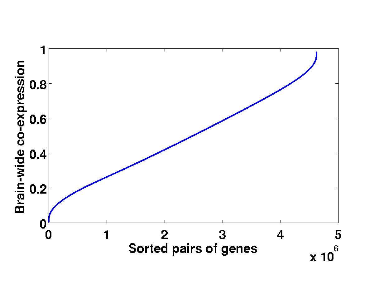
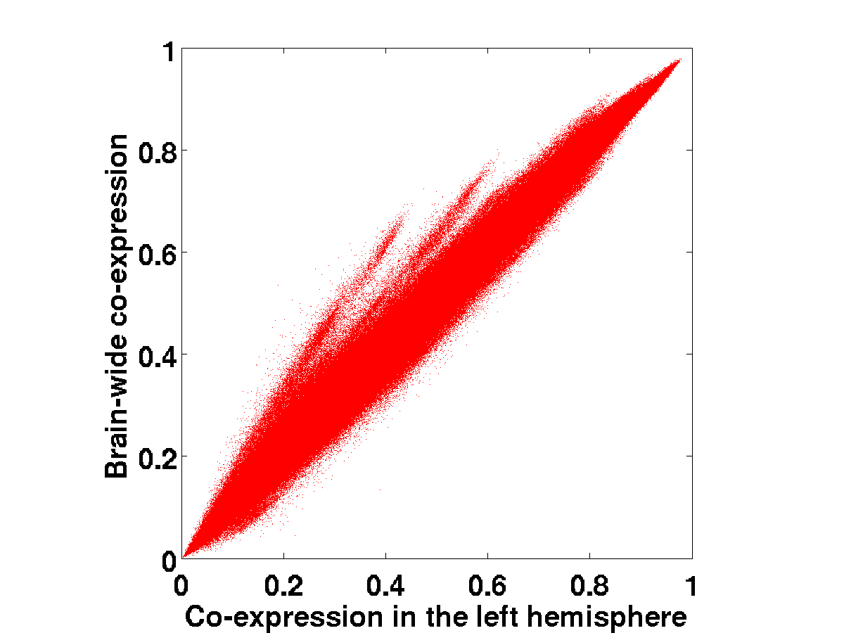
upper_diagonal_coeffs.m, as in the code snipped below, which plots the
distribution of brain-wide co-expression coefficients (Figure 4.1)) and compares it to the one of
co-expression coefficients in the left hemisphere (as defined in the big12
annotation, Figure 4.2).
4.2 Monte Carlo analysis of brain-wide co-expression networks
4.2.1 Special sets of genes versus full atlas
The gene-by-gene matrix defines a universe in which we would like to study co-expression networks of special sets of genes, in a probabilistic way.
| (4.2) |
Given a set of genes of interest, corresponding to the column indices in the data matrix, their co-expression matrix is obtained by extracting the submatrix of corresponding to these indices (see Equation 4.2.4).
| (4.3) |
| (4.4) |
4.2.2 Cumulative distribution function of co-expression coefficients in sets of genes drawn from the Allen Brain Atlas
Having observed (Figure 4.1) that the distribution
of pairwise co-expression coefficients of genes in the whole coronal
atlas is roughly linear in a large domain of co-expression,
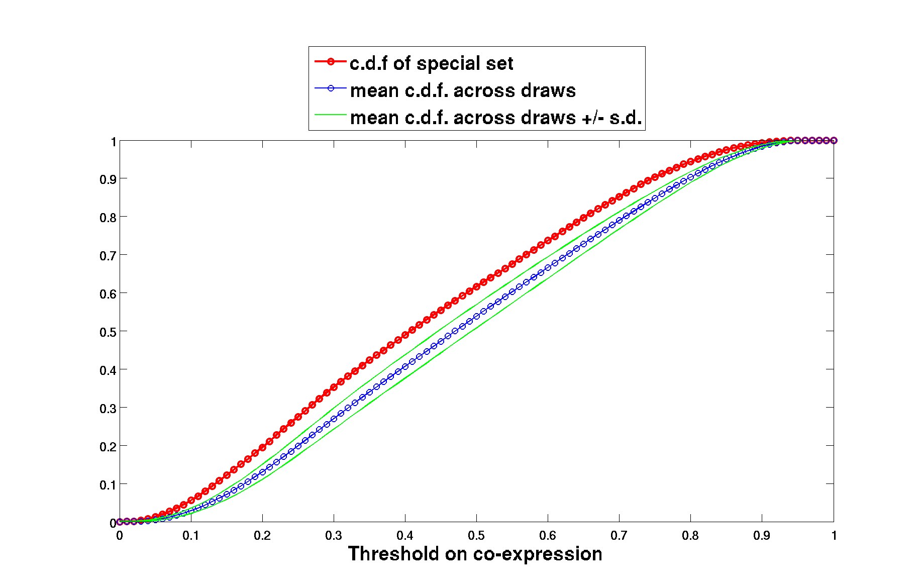
we can study the cumulative distribution
function of the co-expression coefficients in the special set, and compare it
to the one resulting from random sets of genes (with the same number of genes
as the special set, in order to eliminate the sample-size bias).
These cumulative distribution functions are evaluated in the following way. Again let denote the size of the matrix , i.e. the number of genes from which was computed. Consider the set of entries above the diagonal of above the diagonal (which are the meaningful quantities in ):
| (4.5) |
The elements of this set are numbers between 0 and 1. For every number between 0 and 1, the cumulative distribution function (c.d.f.) of , denoted by is defined as the fraction of the elements of that are smaller than this number:
| (4.6) |
where .
For any set of genes, is a growing function and . For highly co-expressed genes, the growth of is concentrated at high values of the argument (in the limit where all the genes in the special set have the same brain-wide expression vector, all the entries of the co-expression matrix go to and the cumulative distribution function converges to a Dirac measure supported at ). To compare the function to what could be expected by chance, let us draw random sets of genes from the Atlas, compute their co-expression network by extracting the corresponding entries from the full co-expression matrix of the atlas (). This induces a family of growing functions on the interval
| (4.7) |
From this family of functions, we can estimate a mean cumulative
distribution function of the co-expression of sets of
genes drawn from the Allen Atlas, by taking
the mean of the values of across the
random draws:
| (4.8) |
Standard deviations of the distribution of c.d.f.s are estimated in the same
way on the interval (which the user of the code can discretize
into a regular grid using the coExprStep component of the options
of the function cumul_co_expr.m, see example below):
| (4.9) |
The functions ,
and
are fields of the output of the function cumul_co_expr.m
whose usage is illustrated in the example below.
Example 21. Cumulative distribution function of co-expression of a special set of genes. Consider the set of 288 genes from the NicSNP database, whose position in the data matrix is encoded in the Matlab file nicotineGenes.mat. NB: the code snippet below can be applied to any special set of genes upon changing the variable indsSmall. It should reproduce Figure 4.3.
4.2.3 Thresholding the co-expression matrix
The co-expression matrix
corresponding to a special subset of the genes in the Allen Atlas (Equation 4.2.4)
is symmetric, like
,
and its entries are in the interval .
It can be mapped to a weighted graph in the following way
(see [6] for details).
The vertices
of the graph are the genes, and the edges are as follows:
- genes and are linked by an edge if their co-expression is strictly positive.
- If an edge exists, it has weight .
Let us define the following thresholding procedure on co-expression graphs: given a threshold between and , put to zero all the entries of that are lower than this coefficient. The underlying graph is obtained by taking the graph corresponding to , and cutting all the links with weight below .
| (4.10) |
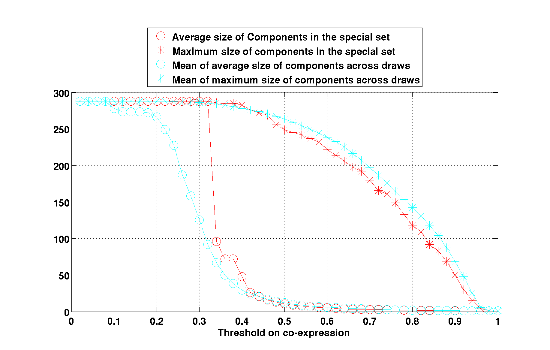
The more-co-expressed a set of genes is, the larger the connected components of the thresholded graphs uderlying will be, for any value of the threshold . For instance we can study the average size of connected components of thresholded co-expression matrices and the size of the largest connected component as a function of the threshold :
| (4.11) |
| (4.12) |
where is the number of connected components with size
. The connected components are worked out using the
implementation of Tarjan’s algorithm [17] in the Matlab function
graphconncomp.m.
4.2.4 Statistics of sizes of connected components
For any quantity worked out from the special co-expression
matrix co-expression matrix
defined in Equation , we can simulate
its probability distribution by repeatedly drawing random
random sets of genes from the atlas,
and recomputing the same quantity on for this set.
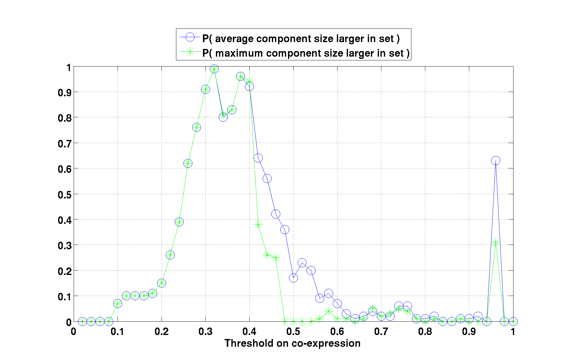
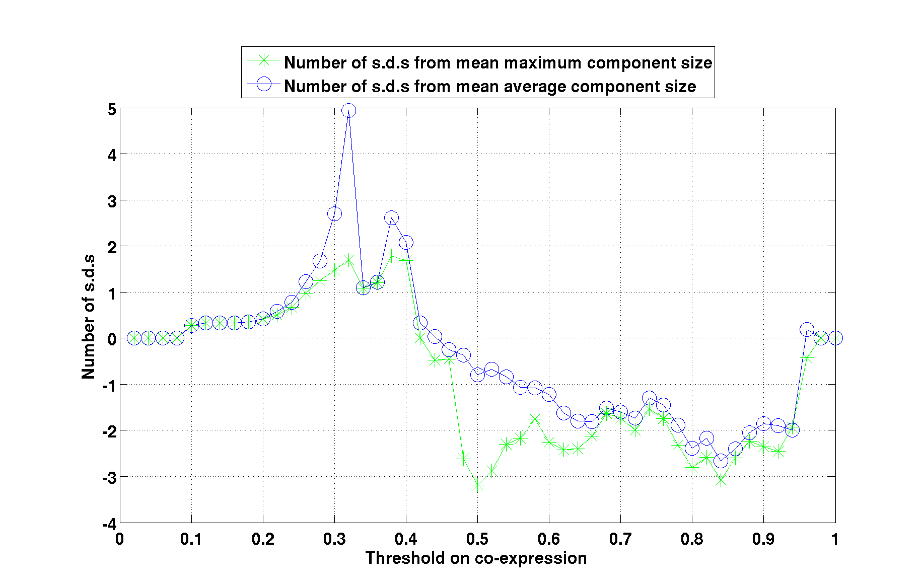
Let us use the above-defined thresholding procedure to study a set of
genes obtained by intersecting the NicSNP
database [16] with the set of genes given
by
get_genes( Ref.Coronal, ’top75CorrNoDup’, ’allen’ ).
We would like to acertain whether this set of genes is more
co-expressed than expected by chance for a set of this size taken
from genesAllen. At each value of a regular
grid the threshold between zero and 1, the function
co_expression_island_bootstrap.m computes
the maximal size and average size of connected components
of the thresholded co-expression graph, and draws random
sets of genes of size from the atlas.
This induces a distribution of partitions of sets
of genes into connected components,
obtained by applying Tarjan’s algorithm to each of the
sets of genes.
Example 22. Consider the set of 288 genes from the NicSNP database, whose position in the data matrix is encoded in the Matlab file nicotineGenes.mat.
4.2.5 Neuroanatomical properties of connected components
Relation between fitting scores and co-expression
If the co-expression of pairs of genes is defined as the cosine of the angle between their expression vectors in voxel space, as in Equation 4.1, the fitting score of a gene to a region of the brain equals the co-expression of gene and a (hypothetical) gene whose expression profile would be proportional to the characteristic function of region :
| (4.13) |
where the second equality comes from the normalization of and in voxel space.
Fitting scores of sums of gene-expression vectors
At a given level of the threshold on co-expression,
a set of genes is partitioned into connected components
induced by the graph underlying the thresholed matrix defined in
Equation . For a set of genes of fixed size numGenes, the function fitting_distribution_in_atlas.m estimates the distribution of fitting scores of the sum of sets of genes of a given size, extracted from the Allen Atlas.
In these functions, the genes are not weighted by coefficients to be optimized, they are simply summed over, so that the set of gene-expression vectors is different from the one explored in marker genes. The fitting score of the sum of genes depends only on a list of distinct genes , and a region in the Allen Reference Atlas:
| (4.14) |
where is the sum of gene-expression vectors of the genes , normalized in the sense:
| (4.15) |
Example 23. Fitting score
of a sum of genes in a given region. It can be computed using
the same functions as for the original data matrix. The sum of the relevant columns of the data matrix has to be substituted to the second argument of the function fitting_from_id.m:
Example 24. Neuroanatomy of nicotine-related genes in the big12 annotation.
One can search the results by -value of fitting scores, and/or size of connected components, and/or brain region:
Example 25. Neuroanatomy
of nicotine-related genes in the big12 annotation (continued).
Chapter 5 Gene-based and cell-based expression data
The computational techniques exposed in this chapter allow to reproduce the results
of [7, 11, 12, 8, 9, 10] (see also [13, 14, 15]
for analyses of the Allen Atlas data in terms of cell types).
5.1 Cell-type-specific microarray data
The file G_t_means.txt contains a matrix of microarray data. The rows correspond to the cell-type-specific samples coming from several studies and analyzed in [18]. The columns correspond to genes (the matrix is a type-by-gene matrix). The following code snippet (included in the file cell_type_start_up.m) defines two matrices with the same numbers of columns, corresponding to the intersection of the sets of genes in the coronal Allen Brain Atlas and in the microarray data:
5.2 Brain-wide correlation profiles
The function cell_types_correls.m computes the voxel-by-type correlation matrix between the coronal Allen Brain Atlas and a set of cell types, as in equation 5.1.
| (5.1) |
| (5.2) |
| (5.3) |
Example 26. Brain-wide correlation profiles
between cell-type-specific data and the Allen Atlas.
To compute the correlations for all the available cell types, the type indices
specified in the variables span the whole range of row indices of the matrix
C:
The results are saved in the file
cellTypesCorrelations.mat. It has rows and
columns (the matrix cellTypesCorrelations is a
voxel-by-type matrix, consistently
with the definition of in Equation 5.1),
so that each column can be mapped to a volume
and visualized in exactly the same way as a column of the data matrix
E:
Example 27. Visualization of brain-wide
correlation profiles. Let us
plot maximal-intensity projections of the correlations between the
20-th row of and all the rows of the Allen Atlas.

5.3 Brain-wide density estimates of cell types
To decompose the gene-expression at every voxel in the Allen Atlas into its cell-type-specific components, let us introduce the positive quantity denoting the contribution of cell-type at voxel , and propose the following linear model:
| (5.4) |
Both sides are estimators of the number of mRNAs for gene at voxel .
The residual term in Equation 5.4 reflects the
fact that cell types are not enough to sample the whole diversity of cell types
in the mouse brain, as well as noise in the measurements, reproducibility
issues, the non-linearity of the relations between numbers of mRNAs,
expression energies and microarray data.
To find the best fit of the model, we have to minimize the residual term by solving the following problem :
| (5.5) |
where
| (5.6) |
As the terms of the sum over voxels that involve a fixed voxel involve only terms of the test function with the same voxel index, and are positive, the problem 5.5 can be solved voxel by voxel. For each voxel we have to minimize a quadratic function of a vector with positive components.
| (5.7) |
For each cell type , the coefficients yield a brain-wide
fitting profile between this cell type and the Allen Atlas.
The function fit_voxels_to_types_picked.m solves the quadratic optimization problems
of Equation 5.7, one per voxel, for a list of cell-type indices, and returns the result in a voxel-by-type
format.
Example 28. Consider the full cell-type-specific dataset with numTypes cell types, and estimate the brain-wide density of each of these cell types:
The result of the computation in the above code snippet
are saved in the file fitVoxelsToTypes.mat. Note that the results
depends on the set of types specified by typeIndicesPicked, since the corresponding
columns of play the role of a basis on which the gene-expression vector at each voxel is
decomposed under positive constraints.
5.4 Cell-type-based computational neuroanatomy
As the matrix of cell-type-specific microarray data is presented
in the type-by-gene format, a given cell type in this dataset corresponds
to a row index in . The corresponding column of any voxel-by-type matrix
(such as correlations , Equation 5.1,
or densities , Equation 5.4)
can be mapped to volumes using the function make_volume_from_labels.m.
Projections of these volume can be visualized
using the function plot_intensity_projections.m. One can
supplement these projections with
sections of these volumes. The sections can be chosen computationally as
follows by ranking the brain regiions in the Allen Reference Atlas using the
brain-wide correlation or density profiles.
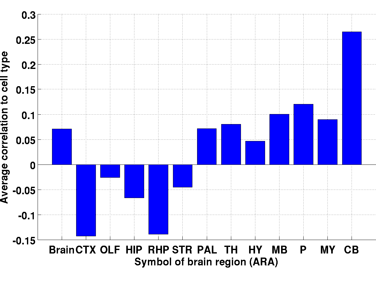
Ranking of regions by correlations with a cell type. Given a three-dimensional grid containing brain-wide correlations between a given cell type and the Allen Atlas (as defined in Equation 5.1), one can rank the regions in a given annotation of the Allen Reference Atlas by computing the average correlation across in each of the regions:
| (5.8) |
For each cell type , each region in the ARA is ranked
according to its average correlation. Call its rank . In particular,
the correlation profile yields a top region in the ARA, for which
. This is the region whose voxels
are most highly correlated to cell type on average.
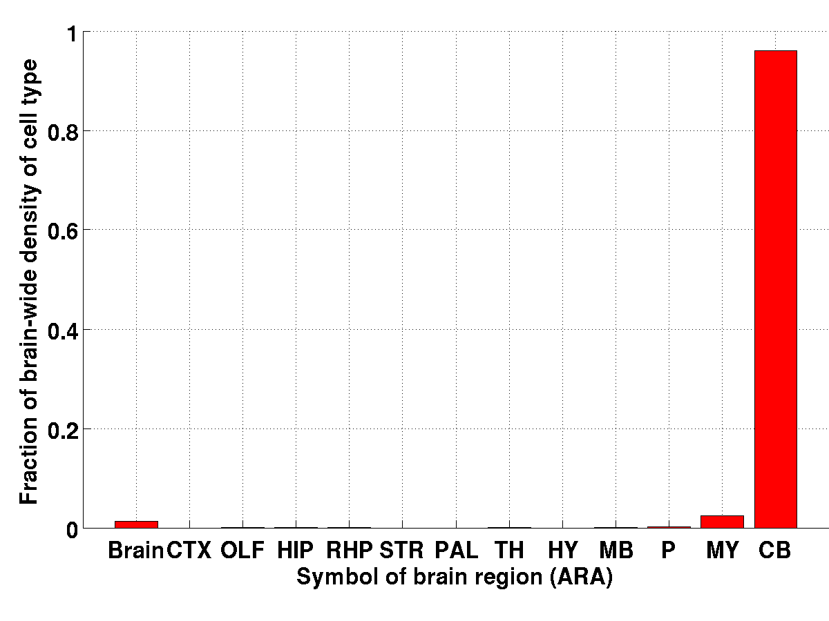
Ranking of regions by estimated density of a cell type. Consider a system of annotation of the ARA, taken from Table 2.1 Big12 is the default option in the Matlab implementation). For each cell-type index and each region (where is an integer index taking values in , where is the number of regions in the chosen system of annotation), we can compute the contribution of the voxels of the region to the brain-wide density profile of cell type :
| (5.9) |
Given a cell type , the regions in the ARA is ranked according to its average
correlation. Call its rank . In particular,
the correlation profile yields a top region in the ARA, for which
. This is the region whose voxels bring the
largest total contribution to the vector .
These two rankings are implemented in the function classify_pattern.m (see example
below). The values of the fraction of total density and average correlation
for a given cell type can be plotted (in the big12 version of the
ARA), using111The labels used in these plots
can be decoded by comparing the fields Ref.Coronal.Annotations.labels{5}
and Ref.Coronal.Annotations.symbols{5}. This yields
the following correspondences: Basic cell groups and regions = Brain,Cerebral cortex = CTX,
Olfactory areas = OLF, Hippocampal region = HIP, Retrohippocampal region = RHP, Striatum = STR,
Pallidum = PAL, Thalamus = TH, Hypothalamus = HY, Midbrain = MB, Pons = P,
Medulla = MY, Cerebellum = CB. the functions plot_correlations_for_big12.m
and plot_densities_for_big12.m.
Example 29. Rank the regions of the big12 annotations by average correlation and fraction of the density of cell types, and display the results for granule cells. The code snippet below should reproduce Figures 5.2 and 5.3.
Given a region in the ARA (our best guess according to one of the above criteria), we need to pick a section that intersects this region. The function cell_type_vol_prepare.m implements the choice of the section. It chooses the section (which can be sagittal, coronal or axial, specified by the field options.sectionStyle of the options) that intersect the desired region (specified by the fields options.identifierIndex and options.regionIndexForSection) along the largest number of voxels, unless the field options.customIndex equals 1. Then it works out the section (of the required style) at a position specified by option.desiredIndex. This function is used by the function figure_for_types.m to produce Figures like 5.4 and 5.5.
5.5 Visualization of correlation and density profiles of cell types
Example 30. Consider the pyramidal neurons, index 47 in the auxiliary dataset. The following code snippet computes the region in big12 annotation of the ARA with the highest average correlation (as in Equation 5.8), and chooses the section of the brain through this section that maximizes the (section-wide) average correlation. It displays it next to the maximal-intensity projections of the correlation profiles, together with a graphical definition of the plane that was used to obtain the section. The snippet should reproduce Figure 5.4 and save it as figureTypeCorrels47.png.

Example 31. Consider again the pyramidal neurons, index 47 in the auxiliary dataset. The following code snippet allows to visualize a section of their estimated brain-wide density, through the region of the ARA that contains the largest fraction of the total density, as per Equation 5.9. It should reproduce Figure 5.5 and save it as figureTypeDensity47.png.

Chapter 6 Clustering
6.1 Kullback–Leibler distance from gene-expression to a given probability distribution
One can use the Kullback–Leibler (KL) divergence to compare the brain-wide expression of
a gene to a given probability distribution over the brain.
This probability distribution can be for instance the normalized average across all genes in the coronal atlas for instance
| (6.1) |
where and are probability densities over the brain obtained by normalization:
| (6.2) |
6.2 Construction of a bipartite graph from a voxel-by-gene matrix
The Allen Atlas can be mapped to a weighted bipartite graph in the following way:
-
•
the first set of vertices consists of voxels, numbered from to ,
-
•
the second set of vertices consists of genes, numbered from to ,
-
•
each of the edges connects one voxel, say to one gene, say and has a weight given by the expression energy of of the gene at the voxel.
We looked for partitions of this weighted bipartite graph into
subgraphs such that the weights of the internal edges of the subgraphs
are strong compared to the weights of the edges between the
subgraphs. This is the isoperimetric problem addressed by the
algorithm of [19] (the graph need not be bipartite to
apply this algorithm, but since we started with a bipartite graph,
each of the subgraphs, or biclusters, returned by the algorithm, is
bipartite, and therefore corresponds to a set of voxels and a set of
genes).
Given a weighted graph, the algorithm cuts some of the links, thus partitioning the graph into a subset and its complementary , such that the sum of weights in the set of cut edges is minimized relative to the total weight of internal edges in . The sum of weights in the set of cut edges is analogous to a boundary term, while the total weight of internal edges is analogous to a volume term. In that sense the problem is an isoperimetric optimization problem, and the optimal set minimizes the isoperimetric ratio over all the possible subgraphs:
| (6.3) |
| (6.4) |
| (6.5) |
| (6.6) |
where the quantity is the weight of the link between vertex and vertex .
Once has been worked out, the algorithm can be applied separately to and its complementary . This
recursive application goes on until the isoperimetric ratio reaches a stopping ratio, representing the
highest allowed isoperimetric ratio. This value is a parameter of the
algorithm. Rising it results in a higher number of clusters, as it rises the number of acceptable cuts.
The implementation of the recursive partition of the bipartite graph
in the present toolbox is due to Grady and Schwartz [19].
Example 32. Partition the left hemisphere of the brain according to the expression of a given set of genes, chosen for their high divergence from a uniform expression. The code snippet below should reproduce Figures LABEL:geneSumBicluster1,geneSumBicluster2,geneSumBicluster3, among other things.


Chapter 7 List of files
7.1 Preparation of data
mouse_start_up.m
cell_type_start_up.m
7.2 Atlas navigation
get_annotation.m
get_genes.m
get_voxel_filter.m
make_volume_from_labels.m
plot_intensity_projections.m
flip_through_sections.m
outline_section_with_atlas_picked.m
annotation_big12_to_fine
annotation_fine_to_big12.m
7.3 Marker genes
localization_from_id.m
localization_scores_region_by_gene.m
fitting_from_id.m
fitting_scores_region_by_gene.m
find_find_lambdamax_l1_ls_nonneg.m (author K. Koh)
l1_ls.m (author K. Koh)
l1_ls_nonneg.m (author K. Koh)
7.4 Co-expression analysis
co_expression_matrix.m
upper_diagonal_coeffs.m
cumul_co_expr.m
cumul_co_expr_plot.m
co_expression_components_bootstrap.m
co_expression_components_bootstrap_plot.m
7.5 Clustering
KL_divergence_from_uniform.m
biclustering_graph_voxel_by_gene.m
bicluster_graph.m
partitiongraph.m (authors: A. Pothen, H. Simon and K.-P. Liou [20])
recursivepartition.m (author: L. Grady)
isosolve.m (author: L. Grady)
7.6 Cell-type specific analysis
cell_type_start_up.m
cell_types_correls.m
fit_voxels_to_types_picked.m
cell_type_vol_prepare.m
classify_pattern.m
figure_for_types.m
figure_for_type_correlations.m
figure_for_type_correlationsdensity.m
plot_correlations_for_big12.m
plot_densities_for_big12.m
7.7 Miscellaneaous operations on matrices
normalise_integral.m.m
normalise_integral_L2.m
7.8 Data files
7.8.1 Allen Brain Atlas, Allen Reference Atlas
refDataStruct.mat
ExpEnergy.mat
ExpEnergytop75percent.mat
7.8.2 Cell-type specific analysis
G_t_means.txt
colsToUseInAllen.mat
colsToUseInTypes.mat
cellTypesDescription.mat
7.9 Saved results
7.9.1 Marker genes
quadTotIdentifier5.mat
quadRegIdentifier5Region1.mat
quadRegIdentifier5Region2.mat
quadRegIdentifier5Region3.mat
quadRegIdentifier5Region4.mat
quadRegIdentifier5Region5.mat
quadRegIdentifier5Region6.mat
quadRegIdentifier5Region8.mat
quadRegIdentifier5Region9.mat
quadRegIdentifier5Region10.mat
quadRegIdentifier5Region11.mat
quadRegIdentifier5Region12.mat
quadRegIdentifier5Region13.mat
7.9.2 Cell-type specific analysis
cellTypesCorrelations.mat
fitVoxelsToTypes.mat
7.9.3 Playground
tool_box_manual_illustration.m
Bibliography
- [1] P. Grange, M. Hawrylycz and P.P. Mitra, Computational neuroanatomy and co-expression of genes in the adult mouse brain, analysis tools for the Allen Brain Atlas, Quantitative Biology, 1(1): 91–100. (DOI) 10.1007/s40484-013-0011-5.
- [2] H.-W. Dong, The Allen reference atlas: a digital brain atlas of the C57BL/6J male mouse, Wiley, 2007.
- [3] E.S. Lein, M. Hawrylycz, N. Ao, M. Ayres, A. Bensinger, A. Bernard, A.F. Boe, M.S. Boguski, K.S. Brockway, E.J. Byrnes, L. Chen, L. Chen, T.M. Chen, M.C. Chin, J. Chong, B.E. Crook, A. Czaplinska, C.N. Dang, S. Datta, N.R. Dee, et al., Genome-wide atlas of gene expression in the adult mouse brain. Nature 445, 168 –176 (2007).
- [4] P. Grange and P.P. Mitra, Computational neuroanatomy and gene expression: optimal sets of marker genes for brain regions, IEEE, in CISS 2012, 46th annual conference on Information Science and Systems (Princeton).
- [5] K. Koh, S.-J. Kim and S. Boyd, An interior-point method for large-scale -regularized logistic regression, Journal of Machine Learning Research 8 (2007) 1519–1555.
- [6] I. Menashe, P. Grange, E.C. Larsen, S. Banerjee-Basu and P.P. Mitra, Co-expression profiling of autism genes in the mouse brain, PLoS computational biology, 9(7), e1003128.
- [7] P. Grange, J.W. Bohland, B.W. Okaty, K. Sugino, H. Bokil, S.B. Nelson, L. Ng, M. Hawrylycz and P.P. Mitra, Cell-type based model explaining coexpression patterns of genes in the brain, PNAS 2014 111 (14) 5397–5402.
- [8] P. Grange, I. Menashe and M. Hawrylycz (2015), Cell-type-specific neuroanatomy of cliques of autism-related genes in the mouse brain. Frontiers in computational neuroscience, 9.
- [9] P. Grange, Computational neuroanatomy: mapping cell-type densities in the mouse brain, simulations from the Allen Brain Atlas, Journal of Physics: Conference Series. IOP Publishing, 2015, 633(1): 012070.
- [10] P. Grange (2015), Cell-type-specific computational neuroanatomy, simulations from the sagittal and coronal Allen Brain Atlas. arXiv preprint arXiv:1505.06434.
- [11] P. Grange, M. Hawrylycz and P.P. Mitra, Cell-type-specific microarray data and the Allen atlas: quantitative analysis of brain-wide patterns of correlation and density, arXiv:1303.0013.
- [12] P. Grange, J.W. Bohland, B.W. Okaty, K. Sugino, H. Bokil, S.B. Nelson, L. Ng, M. Hawrylycz, P.P. Mitra, Cell-type-specific transcriptomes and the Allen Atlas (II): discussion of the linear model of brain-wide densities of cell types, arXiv:1402.2820.
- [13] Ko Y, Ament SA, Eddy JA, Caballero J, Earls JC, Hood L, Price ND (2013) Cell-type-specific genes show striking and distinct patterns of spatial expression in the mouse brain. Proceedings of the National Academy of Sciences, 110(8), 3095–3100.
- [14] Tan PPC, French L, Pavlidis P (2013) Neuron-enriched gene expression patterns are regionally anti-correlated with oligodendrocyte-enriched patterns in the adult mouse and human brain. Frontiers in Neuroscience, 7.
- [15] Li, R., Zhang, W., Ji, S. (2014). Automated identification of cell-type-specific genes in the mouse brain by image computing of expression patterns. BMC bioinformatics, 15(1), 209.
- [16] S.F. Saccone, N.L. Saccone, G.E. Swan, P.A.F. Madden, A.M. Goate, J.P. Rice and L.J. Bierut, Systematic biological prioritization after a genome-wide association study: an application to nicotine dependence, Bioinformatics (2008), 24, 1805–1811.
- [17] R. E. Tarjan, Depth first search and linear graph algorithms, SIAM Journal on Computing, 1(2):146-160, 1972.
- [18] B.W. Okaty, K. Sugino and S.B. Nelson, A Quantitative Comparison of Cell-Type-Specific Microarray Gene Expression Profiling Methods in the Mouse Brain, PLoS One (2011) 6(1).
- [19] L. Grady, E. Schwartz, Isoperimetric partitioning: A new algorithm for graph partitioning, SIAM Journal of Scientific Computing 27 (2006), no. 6, 1844-1866.
-
[20]
A. Pothen, H. Simon and K.-P. Liou, Partitioning Sparse Matrices with Eigenvectors of Graphs (1990), 11, 3, 430–452.