Super-Resolution by Compressive Sensing Algorithms

Abstract - In this work, super-resolution by 4 compressive sensing methods (OMP, BP, BLOOMP, BP-BLOT) with highly coherent partial Fourier measurements is comparatively studied.

An alternative metric more suitable for gauging the quality of spike recovery is introduced and based on the concept of filtration with a parameter representing the level of tolerance for support offset.

In terms of the filtered error norm only BLOOMP and BP-BLOT can perform grid-independent recovery of well separated spikes of Rayleigh index $1$ for arbitrarily large super-resolution factor. Moreover both BLOOMP and BP-BLOT can localize spike support within a few percent of the Rayleigh length. This is a weak form of super-resolution.

Only BP-BLOT can achieve this feat for closely spaced spikes separated by a fraction of the Rayleigh length, a strong form of super-resolution.

I. INTRODUCTION

Superresolution as Fourier spectrum extrapolation (i.e. uncovering high spatial frequency components from low spatial frequency data) is typically an ill-posed process and prone to extreme instability to noise, unless additional prior knowledge and/or multiple data sets are available. Many techniques have been proposed in the literature but few have robust performances and rigorous foundation.

A basic result in super-resolution with Fourier measurements is given by Ref. [3] (see also Ref. [1]). In the present work we discuss the strengths and weaknesses of this result and give a numerical assessment of the super-resolution capability of compressive sensing (CS) algorithms.

First let us review the set-up of Fourier measurements of grid-bound spikes. Consider the noisy Fourier data $y=\Phi x+e$ of a grid-bound spike train

$$x(t)=\sum_{l=0}^{N-1}x(l)\delta(t-\frac{l}{N})$$ (1)

on a fine grid of spacing $N^{-1}$ with the sensing matrix element

$$\Phi_{kl} =e^{-2\pi ikl/N},\quad k\in[0,N/F).$$ (2)

When $F>1$, one is confronted with the problem of retrieving the fine scale structure of $x$ from a coarse scale information only. The Rayleigh resolution length $\ell$ associated with the Fourier data is the reciprocal of the observed bandwidth in (2). The ratio $F$ of the Rayleigh length to the fine grid spacing is the super-resolution factor Ref. [1, 3] or the refinement factor Ref. [4, 5].

According to Ref. [3], any grid-bound spike train of the form (1) that is consistent with the Fourier data over the frequency band $[0,N/F)$ deviates from the true solution by

$$\hbox{Error $\leq$ Constant $\cdot F^{\alpha}\cdot$ Noise},\quad\alpha\leq 2R+1$$ (3)

where

$$R(S)=\min\left\{r:r\geq\sup_{t}\#(S\cap[t,t+4\ell r))\right\}$$ (4)

is the Rayleigh index of the support set $S$ of $x$. As explained in Ref. [3], a set has Rayleigh index at most $R$ if in any interval of length 4$\ell\cdot R$ there are at most $R$ spikes.

To increase $R$, one can decrease the minimum distance and/or increase the number of spikes separated below $4\ell$ on (local) average. The power $\alpha$ measures the degree of noise amplification by super-resolution.

Recently Ref. [1], an error bound like (3) with $\alpha=2$ is established for reconstruction of spikes separated by at least $4\ell$ (thus $R=1$) by convex programming analogous to Basis Pursuit (BP) Ref. [2] with Fourier data sampled at integers $k$ of the band $[0,N/F)$.

The above sensing set-up, however, has the following two drawbacks.

II. GRID-INDEPENDENT CS

The first drawback is that when the prior information of grid-bound spikes is not available, then imposing such a model assumption can lead to poor reconstruction.

To reduce the gridding error due to off-grid objects one can reduce the grid spacing. But to resolve the finer grids, one must increase the received bandwidth which in turn brings the gridding error back to the original level and defeats the purpose of grid refinement. The same problem arises in radar imaging when the probe wavelengths are larger than the sizes of the off-grid scatterers. Often brushed off in literature Ref. [6, 7], this issue is particularly pertinent to sparsity-based imaging schemes relying on accurate and sparse representation of the objects which, in view of the intrinsically discrete nature of CS framework, may be utterly untenable for imaging in continuum.

How to get out this conundrum? Recently we have developed a solution method based on the techniques of coherence Band exclusion and Local Optimization (acronym: BLO) Ref. [5] which introduces a more refined notion of local coherence bands.

Roughly speaking the idea is this: Let the standard grid spacing be the Rayleigh resolution length $\ell$ and the refined grid spacing be $\ell^{\prime}<\ell$. When the super-resolution factor $F=\ell/\ell^{\prime}$ is large, the nearby columns are nearly parallel, forming the coherence bands. The size of the coherence band is approximately twice the Rayleigh length. Due to the presence of coherence bands, the mutual coherence of the sensing matrix is close to one, leading to a poor condition number of even small column sub-matrices. As expected standard CS methods break down in this situation.

If, however, the spikes are separated by at least $\ell$ then spikes do not fall into the coherence band of one another. So if one searches the next object outside the coherence bands of the previously identified objects by a greedy algorithm, say Orthogonal Matching Pursuit (OMP), then the coherence bands would not get in the way of reconstruction. This is the technique of coherence band exclusion.

To improve the accuracy of reconstruction, one can further zoom in within coherence bands of the recovered objects one at a time by locally minimizing the residual which is inexpensive computationally. This is the technique of local optimization (see Algorithm 1).

Algorithm 1. Local Optimization (LO)
Input:$\Phi,y,S^{0}=\{i_{1},\ldots,i_{k}\}$.
Iteration: For $n=1,2,...,k$.
1) $x^{n}=\hbox{arg}\,\,\min_{z}\|\Phi z-y\|,$
$\hbox{supp}(z)=(S^{n-1}\backslash\{i_{n}\})\cup\{j_{n}\},$
$j_{n}\in\hbox{Band}(\{i_{n}\})$.
2) $S^{n}=\hbox{supp}(x^{n})$.
Output: $S^{k}$.

Remark 1.

For spikes separated by at least $\ell$, the “Band($\{j_{n}\}$)” in Algorithm 1 is the set of indices within the distance $\ell$ from $\{j_{n}\}$. For spikes separated by less than $\ell$, “Band($\{j_{n}\}$)” is the set of indices within half the minimum separation of spikes. In the latter situation, the algorithm requires the prior knowledge of the minimum separation of spikes.

The same remark applies to Algorithms 2 and 3 below.

In Ref. [5] we have obtained performance guarantee for the BLO-based greedy algorithm, BLOOMP (standing for BLO-based OMP), which can recover the support of spikes separated by at least $3\ell$ within the accuracy of one $\ell$ (as measured by the Bottleneck distance) independent of the super-resolution factor. In reality, the accuracy of the support estimate is just a few percent of the Rayleigh length $\ell$ (see below). Note that spikes separated by at least $3\ell$ can comprise a set of arbitrarily large Rayleigh index.

Moreover, this grid-independent performance can be achieved with sparse measurements, leading to grid-independent CS. The numerical performances of BLOOMP and other variants have been thoroughly and systematically tested in Ref. [5].

Algorithm 2. BLOOMP

Input: $\Phi,y,s=\hbox{\rm sparsity (number of spikes)}$

Initialization: $x^{0}=0,r^{0}=y$ and $S^{0}=\emptyset$

Iteration: For $n=1,...,s$

1) $i_{\rm max}=\hbox{arg}\max_{i}|\Phi_{i}^{*}r^{n-1}|,i\notin\hbox{\rm Band}(S^{n-1})$

2) $S^{n}=\hbox{LO}(S^{n-1}\cup\{i_{\rm max}\})$

where LO is the output of Algorithm 2.

3) $x^{n}=\hbox{arg}\min_{z}\|\Phi z-y\|$ s.t. supp($z$) $\in S^{n}$

4) $r^{n}=y-\Phi x^{n}$

Output: $x^{s}$.

When the BLO technique is combined with thresholding we have the Band-excluded, Locally Optimized Thresholding (BLOT) which can be used to enhance the performance of BP. The BLOT-enhanced BP is called BP-BLOT (see Algorithm 3).

Algorithm 3. BLOT

Input: $x$, $\Phi,y,s=\hbox{\rm sparsity (number of spikes)}$.

Initialization: $S^{0}=\emptyset$.

Iteration: For $n=1,2,...,s$.

1) $i_{n}=\hbox{arg}\,\,\max_{j}|x_{j}|,j\not\in\hbox{Band}(S^{n-1})$.

2) $S^{n}=S^{n-1}\cup\{i_{n}\}$.

Output:

$\hat{x}=\hbox{arg}\min\|\Phi z-y\|_{2}$, $\hbox{supp}(z)\subseteq\hbox{LO}(S^{s}),$

where LO is the output of Algorithm 1.

Note that BLOOMP and BP-BLOT require the prior information of the sparsity.

III. FILTERED ERROR METRIC

The second drawback of (3) is that the discrete norm used in (3) does not take into account of the degree of separation between the estimated support and the true support as measured by the Hausdorff distance or the Bottleneck distance. The discrete norm treats any amount of support offset equally.

An easy remedy to the injudicious treatment of support offset is to use instead the filtered error norm $\|\hat{x}_{\eta}-x_{\eta}\|,$ where $x_{\eta}$ and $\hat{x}_{\eta}$ are, respectively, $x$ and $\hat{x}$ convoluted with an approximate delta-function of width $2\eta$.

If every spike of $\hat{x}$ is within $\eta$ distance from a spike of $x$ and if the amplitude differences are small, then the $\eta$-filtered error is small. The filter parameter $\eta$ represents the level of tolerance for the support off-set in a specific context. The filtered error plot, as $\eta$ and noise level vary, will give a more accurate and complete picture of the super-resolution effect. We will demonstrate the utility of the filtered norm in the numerical tests.

IV. NUMERICAL TESTS

(a) OMP

(b) BLOOMP

(c) BP

(d) BP-BLOT

Figure 1: Reconstructions of the real part of 20 randomly phased spikes with $R=1$ (minimum distance $4\ell$), $F=50,\hbox{\rm SNR}=20$.

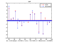
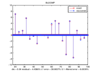
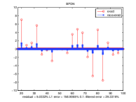
In all our tests, we use $150\times N$ partial Fourier matrices (2) where $N=150F$ for various $F$ and $k=0,1,2,\cdots,149.$ In this setting, $\ell=1/150$.

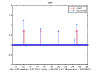
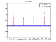
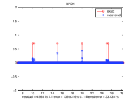
For a demonstration of grid-independent recovery, Fig.1 shows reconstructions of 20 spikes separated by at least $4\ell$ ( $R=1$) by using OMP, BP, BLOOMP and BP-BLOT with noisy ($5\%$) Fourier data. For this simulation, $F=50$. We use the open-source code YALL1 (http://yall1.blogs.rice.edu/) to find the BP solution.

In this test, OMP tends to miss small spikes. BLOOMP, however, approximately recover the support and magnitudes of the spikes. While the BP reconstruction tends to cluster around the true spikes, BP-BLOT dramatically improves the performance. BLOOMP and BP-BLOT have a similarly superior performance which is essentially independent of $F$. BLOOMP and BP-BLOT also perform much better than other existing schemes (see Ref. [5, 4] for systematic comparison).

More quantitatively, the BLO technique reduces the unfiltered error 144% and $0.1$-filtered error 45% for OMP to 39% and 6%, respectively, for BLOOMP. The BLOT technique reduces the unfiltered error 159% and $0.1$-filtered error 29% for BP to 39% and 6%, respectively, for BP-BLOT.

(a) SNR=100, $\eta=0$

(b) SNR=100, $\eta=0.05\ell$

(c) SNR=20, $\eta=0$

(d) SNR=20, $\eta=0.05\ell$

(e) SNR=10, $\eta=0$

(f) SNR=10, $\eta=0.05\ell$

Figure 2: Relative errors in reconstruction by OMP, BLOOMP, BP and BP-BLOT versus the super-resolution factor.

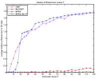
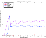
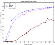
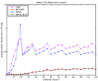
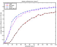
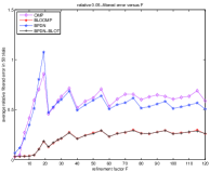
Fig.2 shows the filtered error with $\eta=0\&0.05\ell$ versus $F$ for $20$ well separated spikes with $1,5,10\%$ Gaussian noises. It is noteworthy that the error curves for OMP and BP are essentially independent of SNR when $F\geq 15$. This may be due to the sensitivity of the algorithms to the round-off error for large $F$.

Also, the power-law amplification (PLA) regimes for OMP and BP are not affected by the filtration with $\eta=0.05\ell$. The PLA regime for BP is about $F<20$ ($F<5$ for OMP) while the PLA regimes for BLOOMP and BP-BLOT are much milder and slower growing.

If we set the relative error equal to, say thrice the noise level as the threshold of successful recovery, then in terms of either the unfiltered or filtered error OMP and BPDN fail for $F>10$ while BLOOMP and BP-BLOT succeed for all $F$ in terms of the filtered error, achieving grid-independent recovery. This remains true for a lower error threshold if the filtration parameter $\eta$ is increased.

(a) OMP

(b) BLOOMP

(c) BP

(d) BP-BLOT

Figure 3: Reconstructions of 5 randomly phased spikes located at $76,76.5,79,80,81\ell$ ($R=5$) with $F=50,\hbox{\rm SNR}=20$.

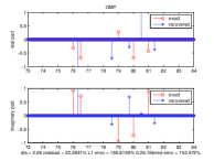
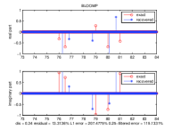
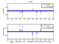
Next we test the strong form of super-resolution with spikes separated by sub-Rayleigh length. As mentioned before, in this case the spikes can fall into one another’s coherence band, thus confusing the recovery. In this case the excluded zones in Algorithms 1, 2 and 3 are not coherence bands of previously detected spikes but smaller zones whose size is set to be half the least separation of spikes (Remark 1). Again we set $F=50$ and SNR=20.

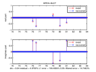
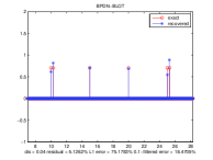
Fig.3 shows the reconstructions of 5 randomly phased spikes ($S=\{76,76.5,79,80,81\ell\}$) while Fig.4 shows the reconstructions of 6 complex spikes of positive real parts ($S=\{10,10.3,15,20,25,25.3\ell\}$) by OMP, BP, BLOOMP and BP-BLOT. According to the definition (4) the former set has Rayleigh index 5 and the latter set has Rayleigh index 6. Clearly, only BP-BLOT performs reasonably well in both cases.

Several observations are in order. First, when some spikes are separated by less than $\ell$, the BLO technique may not improve on the OMP reconstructions. Second, the BLOT technique improves on the BP reconstructions, especially for the Bottleneck distance of support offset, achieving the accuracy of $0.04\ell$ in both Fig.3 and Fig.4. Third, the filtered errors for BP-BLOT (15% with $\eta=0.25\ell$ in Fig.3(d) and $18\%$ with $\eta=0.1\ell$ in Fig.4(d)) are much smaller than the unfiltered errors (199% in Fig.3(d) and 75% in Fig.4(d)). Fig.3 (d) most clearly demonstrates the inadequacy of the unfiltered norm as the error metric for spike recovery.

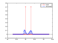
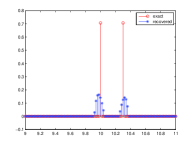
Zooming in on the two pairs of closely spaced spikes in Fig.4(c) will give us a better sense of how the BLOT technique achieves the feat of super-resolution (see Fig.5). BLOT capitalizes on the tendency of BP spikes to mushroom around the true spikes and use the extra prior information (sparsity and minimum separation) to prune and grow the reconstruction.

Finally, unlike the case of Rayleigh index 1 in Fig.1, the BLOT technique slightly increases the residuals (from 4.97% to 4.98% in Fig.3 and 4.99% to 5.13% in Fig.4) to achieve the super-resolution effect. In contrast, the BLO technique always reduces the residuals which may not help recovery of spikes separated by sub-Rayleigh length.

(a) OMP

(b) BLOOMP

(c) BP

(d) BP-BLOT

Figure 4: Reconstructions of the real parts of 5 complex spikes located at $10,10.3,15,20,25,25.3\ell$ ($R=6$) with $F=50,\hbox{\rm SNR}=20$.

V. CONCLUSION

We have argued that the discrete unfiltered norm is not a proper error metric for spike recovery since the offset of the support recovery is not accounted for and that a filtered error norm may be used instead.

We have demonstrated that both BLOOMP and BP-BLOT can recover well separated spikes in terms of the filtered error norm as well as localize the spikes within a few percent of the Rayleigh length, independent of the super-resolution factor. This is a weak form of super-resolution.

When some spikes are closely spaced below the Rayleigh length, only BP-BLOT can localize the spikes within a few percent of $\ell$. The performance can be further enhanced by increasing the number of Fourier data within the same bandwidth, moving from the under-sampling to the full and even over-sampling regimes (not shown).

Our numerical tests show that the super-resolution factor and the Rayleigh index are not the only factors at play. The minimum separation, the range of spike values and overall configuration also affect super-resolution results.

(a) spikes at 10, 10.3$\ell$

(b) spikes at 25, 25.3$\ell$

Figure 5: Zoom-ins of the closely spaced spikes in Fig.4(c).

REFERENCES

- [1] E.J. Candès and C. Fernandez-Granda, “Towards a mathematical theory of super-resolution,”preprint, 2012.
- [2] S.S. Chen, D.L. Donoho and M.A. Saunders, “Atomic decomposition by basis pursuit,” SIAM Rev. Vol. 43, pp.129-159, 2001.
- [3] D.L. Donoho, “Superresolution via sparsity constraints,”SIAM J. Math. Anal. Vol. 23, pp. 1309-1331, 1992.
- [4] A. Fannjiang and W. Liao, “ Mismatch and resolution in compressive imaging,” Wavelets and Sparsity XIV, edited by Manos Papadakis, Dimitri Van De Ville, Vivek K. Goyal, Proc. of SPIE Vol. 8138, 2011.
- [5] A. Fannjiang and W. Liao, “Coherence-pattern guided compressive sensing with unresolved grids,”SIAM J. Imaging Sci. Vol. 5, pp. 179-202, 2012.
- [6] S. Gazit, A. Szameit, Y. C. Eldar, M. Segev, “Super-resolution and reconstruction of sparse subwavlength images,” Opt. Exp. Vol. 17, pp. 23920-23946, 2009.
- [7] A. Szameit et al.,“Sparsity-based single-shot subwavelength coherent diffractive imaging,” Nat. Mat. Vol. 11, pp. 455 - 459, 2012.