Drell-Yan lepton pair production at high energies in the Parton Reggeization Approach

Abstract

According to extensive theoretical studies of the high energy limit of QCD, inelastic interactions are dominated by the multi-Regge final states. The appropriate gauge-invariant objects, which simultaneously incorporate the transverse momentum degrees of freedom, are Reggeized gluons, quarks and antiquarks. In the present communication we extend parton Reggeization approach to Drell-Yan production of massive lepton pairs. The basic ingredient is a process of Reggeized quark-antiquark annihilation, ${\cal Q}\bar{\cal Q}\to\gamma^{\star}\to l^{+}l^{-}$, which is described by the Reggeon-Reggeon-photon effective vertex $\Gamma^{\gamma}_{{\cal Q}\bar{\cal Q}}$. We calculate transverse-momentum and invariant-mass distributions of Drell-Yan lepton pairs measured at the CERN SPS, FNAL Tevatron and CERN LHC in the different ranges of energy and rapidity. We focus on angular distributions of Drell-Yan leptons in different kinematical ranges. The obtained results are compared with the existing data and a good agreement is found. The predictions for future experiments for Drell-Yan lepton pair production at the CERN LHC have been made.

I Introduction

The Drell-Yan production of lepton pairs, the principal QCD subprocess for which is an annihilation of quarks and antiquarks from colliding hadrons into lepton pairs DrellYan , is not only a supplement to the standard deep inelastic (DIS) studies. Drell-Yan production stands out as an important source of the experimental data on the flavor content of the nucleon sea (see NuSea and references therein). More recently there has been much discussion of the Drell-Yan production as a unique source of the direct information on fine spin properties of the proton, including transversity and a new family of transverse-momentum dependent (TMD) structure functions TMD1 ; TMD2 .

On the discovery frontier, Drell-Yan process emerges as a background to heavy vector-meson production in the Standard Model (SM) and beyond, as Drell-Yan lepton pairs with mass above the $Z-$bosom mass are a major background in searches for new heavy vector mesons. Finally, Drell-Yan production at the LHC would probe parton distribution functions (PDFs) at very small $x$, down to $x\simeq 10^{-6}$. The experimental studies of Drell-Yan lepton pair production include measurements of rapidity ($y$), invariant mass ($Q$), transverse momentum ($q_{T}=|{\vec{q}}_{T}|$) of lepton pairs, and angular distributions of leptons in the virtual photon rest frame.

Theoretical study of Drell-Yan lepton pair production in the perturbative Quantum Chromodynamics (pQCD) framework is in a very advanced state and extends from the leading-order (LO) to next-to-leading-order (NLO) approximations in the strong coupling constant $\alpha_{s}$ Stirling ; Review ; Berger1 to the soft initial-state gluon resummation procedure to all orders in $\alpha_{s}$ (see Resum ; Berger2 and references therein).

Ever since the pioneering works by Dokshitser et al. DDT and Altarelli et al. Altarelli there has been much work of the $q_{T}-$distribution of lepton pairs in the framework of standard collinear factorization with on-mass shell partons (see Stirling ; Review ; Berger1 ; Resum ; Berger2 and references therein). More recent activity on $q_{T}-$distributions, which goes beyond the collinear approximation, focused on TMD’s Boer . The often discussed $k_{T}-$factorization with off-shell mass partons is a part of such approach. At small-x of our interest the principal ingredients are off-shell properties of $t-$channel exchanges and unpolarized unintegrated parton distribution functions (PDF)KT1 ; KT2 . Indeed, at a deeper level of high energy pQCD, quarks, antiquarks and gluons are known to reggeize Lipatov95 ; BFKL ; FadinSherman ; FadinLipatov . Furthermore, as has been shown by Lipatov and collaborators, Reggeized gluons and quarks are the appropriate gauge-invariant degrees of freedom of high-energy pQCD. In the practical applications, the use of Reggeized $t-$channel exchanges is justified by the dominance of the so-called multi-Regge final states in inelastic collisions of high energy hadrons.

Earlier, the quark Reggeization hypothesis has been used successfully for a description of different spectra of prompt photons at the Fermilab Tevatron and CERN LHC tevatronY ; tevatronYY ; lhcY , electron deep inelastic scattering and prompt photon production cross sections at the DESY HERA tevatronY ; heraY , and forward $Z-$boson production cross section at the CERN LHC HautmanZ . In the present communication we discuss the experimental data for proton-proton and proton-antiproton collisions including the Fermilab Tevatron experiments DY_CDF ; DY_D0 ; NuSea and the CERN SPS experiments R209 ; UA1 , and new data from the CERN LHC CMSDY ; LHCbDY .

This paper is organized as follows: In Sec. II, the general formalism for description of Drell-Yan lepton pair production is presented. In Sec. III, we calculate helicity structure functions in the LO of Parton Reggeization Approach (PRA) and obtain master formulas for lepton pair spectra and angular coefficients. In Sec. IV, we present results of our calculations for invariant-mass and transverse-momentum spectra of Drell-Yan lepton pairs and report a comparison with relevant experimental data from the Fermilab Tevatron, CERN SPS and CERN LHC. We also compare our predictions with the data for angular coefficients and predict transverse-momentum dependence of the angular coefficients in the energy range of the CERN LHC, $\sqrt{S}=7-14$ TeV. Section V contains our conclusions.

II Drell-Yan pair production in QCD and PRA

According to the perturbative QCD Parton Model the LO subprocess of Drell-Yan lepton pair production is an annihilation of quark and antiquark from the colliding hadrons into the virtual photon which decays onto lepton pair:

$$q+\bar{q}\to\gamma^{\star}\to l^{+}+l^{-}.$$ (1)

In this formalism the quark and antiquark in an initial state have zero transverse momentum with respect to the hadron collision axis and massive lepton pair (or virtual photon) is produced with zero transverse momentum. The angular distribution of leptons in the virtual photon rest frame should be

$$\frac{dN}{d\cos\theta}\sim 1+\cos^{2}\theta,$$ (2)

where $\theta$ is the polar angle of the lepton relative to the collision axis. Experimentally, massive lepton pairs are produced with substantial transverse momentum ${q}_{T}$. To describe Drell-Yan lepton pairs with nonzero transverse momentum, within the collinear Parton Model one invokes the NLO partonic subprocesses $2\to 2$, which are of the first order in $\alpha_{s}$:

$$q+\bar{q}\to g+\gamma^{\star}\to g+l^{+}+l^{-},$$ (3)

$$q+g\to q+\gamma^{\star}\to q+l^{+}+l^{-},$$ (4)

where $g$ is the Yang-Mills gluon. It is obvious, that in these subprocesses the lepton angular distribution will differ from the trivial form (2). If the colliding hadrons were polarized, their polarization transfer to the initial partons and angular distributions of the final leptons will change respectively. In framework of the NLO QCD and the collinear Parton Model, the Drell-Yan lepton pair production in collisions of polarized and unpolarized hadrons have been studied carefully, with exception of only the regions of small $q_{T}$ and $Q$ Stirling ; Review ; Berger1 .

In the $k_{T}-$factorization approach KT1 ; KT2 , the off-shell initial partons $(q^{*},g^{*})$ of nonzero transverse momenta are considered from the beginning. Instead of processes (3) and (4), the relevant LO and NLO contributions are

$$q^{*}+\bar{q}^{*}\to\gamma^{\star}\to l^{+}+l^{-},$$ (5)

$$q^{*}+\bar{q}^{*}\to g+\gamma^{\star}\to g+l^{+}+l^{-},$$ (6)

$$q^{*}+g^{*}\to q+\gamma^{\star}\to q+l^{+}+l^{-}.$$ (7)

However, one must be careful with off-shell quarks and antiquarks as one may break the gauge invariance of relevant amplitudes and break the electromagnetic current conservation. The additional problem of the $k_{T}-$factorization calculations is a double counting, when subprocesses (5), (6) and (7) are taken into account together. These difficulties can be solved in PRA, where the initial off-shell gluons and quarks are considered as Reggeons or Reggeized gluons and quarks, which interact with usual quarks and Yang-Mills gluons in a special way, via gauge invariant effective vertices which incorporate the initial and final state radiation effects on equal footing FadinLipatov ; FadinSherman ; Antonov ; LipatoVyazovsky . Our previous studies of inclusive jet lhcY , and inclusive prompt photon production tevatronY ; heraY have shown that in PRA it is sufficient to consider only LO $2\to 1$ subprocess for a good quantitative description the experimental data.

In PRA, the LO subprocess, which describes finite $q_{T}$ Drell-Yan lepton pairs, is an annihilation of Reggeized quark and Reggeized antiquark via virtual photon:

$${\cal Q}(q_{1})+\bar{\cal Q}(q_{2})\to\gamma^{\star}\to l^{+}(k_{1})+l^{-}(k_{2}).$$ (8)

The amplitude of the subprocess (8) reads as follows

$$M({\cal Q}_{i}\bar{\cal Q}_{i}\to l^{+}l^{-})=4\pi\alpha e_{i}\bar{V}(x_{2}P_{2})\Gamma^{\gamma,\mu}_{{\cal Q}\bar{\cal Q}}(q_{1},q_{2})U(x_{1}P_{1})\otimes\bar{U}(k_{1})\gamma_{\mu}V(k_{2}),$$ (9)

where $e_{i}$ is the electric charge of quark $i$ (in units of electron charge), $\alpha$ is the electromagnetic constant, and $\Gamma^{\gamma,\mu}_{{\cal Q}\bar{\cal Q}}(q_{1},q_{2})$ is the Fadin-Sherman effective vertex FadinSherman ; LipatoVyazovsky ,

$$\Gamma^{\gamma,\mu}_{{\cal Q}\bar{\cal Q}}(q_{1},q_{2})=\gamma^{\mu}-\frac{2\hat{q}_{1}P_{1}^{\mu}}{x_{2}S}-\frac{2\hat{q}_{2}P_{2}^{\mu}}{x_{1}S}.$$ (10)

It is easy to show that the amplitude (9) is gauge invariant and $\Gamma^{\gamma,\mu}_{{\cal Q}\bar{\cal Q}}(q_{1},q_{2})(q_{1}+q_{2})_{\mu}\equiv 0$. Four-momenta of Reggeized quarks (antiquarks) have transverse components and they read $q_{i}^{\mu}=x_{i}P_{i}^{\mu}+q_{iT}^{\mu}$, $q_{iT}^{\mu}=(0,\vec{q}_{iT},0)$, $q_{i}^{2}=q_{iT}^{2}=-\vec{q}_{iT}^{~{}2}=-t_{i}\neq 0$.

The Drell-Yan pair production in the proton-proton and proton-antiproton high-energy collisions corresponds to the following processes

$$p(P_{1})+\bar{p}(P_{2})\to l^{+}(k_{1})+l^{-}(k_{2})+X,$$ (11)

$$p(P_{1})+p(P_{2})\to l^{+}(k_{1})+l^{-}(k_{2})+X,$$ (12)

where four-momenta of particles are shown in brackets, $l=e,\mu$ (electron or muon), $q=q_{1}+q_{2}=k_{1}+k_{2}$ is the four-momentum of virtual photon, $Q=\sqrt{q^{2}}$ and $Q_{T}^{2}=Q^{2}+{\vec{q}}_{T}^{~{}2}=x_{1}x_{2}S$. Differential cross section for processes (11) and (12) have the standard form:

$$\frac{d\sigma}{d^{4}qd\Omega}=\frac{\alpha^{2}}{32\pi^{4}SQ^{4}}L_{\mu\nu}W^{\mu\nu}$$ (13)

or

$$\frac{d\sigma}{dQ^{2}dq_{T}^{2}dyd\Omega}=\frac{\alpha^{2}}{64\pi^{3}SQ^{4}}L_{\mu\nu}W^{\mu\nu},$$ (14)

where $y$ is the rapidity of virtual photon (or $l^{+}l^{-}$ lepton pair), $d\Omega=d\phi d\cos\theta$ is the spatial angle of producing positive lepton in the rest frame of virtual photon, $P_{1}=\frac{\sqrt{S}}{2}(1,0,0,1)$, $P_{2}=\frac{\sqrt{S}}{2}(1,0,0,-1)$, $\sqrt{S}$ is the total energy of colliding particles. Here

$$L^{\mu\nu}=2(k_{1}^{\mu}k_{2}^{\nu}+k_{1}^{\nu}k_{2}^{\mu})-Q^{2}g^{\mu\nu}$$ (15)

is the leptonic tensor, whereas

$$W_{\mu\nu}=\int d^{4}xe^{iqx}\langle P_{1}P_{2}|j_{\mu}(x)j_{\nu}(0)|P_{1}P_{2}\rangle$$ (16)

is the hadronic tensor.

The convolution of hadronic and leptonic tensors reads as a sum of contributions of the so-called helicity structure functions $W_{T,L,\Delta,\Delta\Delta}$ Berger2 ; helicityDY :

$$\frac{d\sigma}{dQ^{2}dq_{T}^{2}dyd\Omega} = \frac{\alpha^{2}}{64\pi^{3}SQ^{2}}\Bigl{[}W_{T}(1+\cos^{2}\theta)+W_{L}(1-\cos^{2}\theta)+$$ (17)

$$+ W_{\Delta}\sin 2\theta\cos\phi+W_{\Delta\Delta}\sin^{2}\theta\cos 2\phi\Bigr{]}.$$

After integration over the angles $\theta$ and $\phi$ in (17), we obtain

$$\frac{d\sigma}{dQ^{2}dq_{T}^{2}dy} = \frac{\alpha^{2}}{64\pi^{3}SQ^{2}}\left(\frac{16\pi}{3}\right)W_{TL},$$ (18)

where $W_{TL}=W_{T}+W_{L}/2$. In the analysis of experimental data, the angular distribution of leptons is represented in terms of two sets of the angular coefficients:

$$\frac{dN}{d\Omega} = (1+\cos^{2}\theta)+A_{0}\left(\frac{1}{2}-\frac{3}{2}\cos^{2}\theta\right)+A_{1}\sin 2\theta\cos\phi+\frac{A_{2}}{2}\sin^{2}\theta\cos 2\phi$$ (19)

and

$$\frac{dN}{d\Omega} = \frac{4}{\lambda+3}\left(1+\lambda\cos^{2}\theta+\mu\sin 2\theta\cos\phi+\frac{\nu}{2}\sin^{2}\theta\cos 2\phi\right),$$ (20)

with the normalization

$$\int\left(\frac{dN}{d\Omega}\right)d\Omega=\frac{16\pi}{3}.$$ (21)

One set consists of the coefficients

$$A_{0}=\frac{W_{L}}{W_{TL}},\quad A_{1}=\frac{W_{\Delta}}{W_{TL}},\quad A_{2}=\frac{2W_{\Delta\Delta}}{W_{TL}},$$ (22)

and the other one is defined by

$$\lambda=\frac{2-3A_{0}}{2+A_{0}},\quad\mu=\frac{2A_{1}}{2+A_{0}},\quad\nu=\frac{2A_{2}}{2+A_{0}}.$$ (23)

Helicity structure functions are obtained by the projection of hadronic tensor on the photon states with the different polarizations $\epsilon_{\lambda}^{\mu}(q)$, $\lambda=\pm 1,0$:

$$W_{T} = W_{\mu\nu}\epsilon_{+1}^{\mu\star}\epsilon_{+1}^{\nu},$$ (24)

$$W_{L} = W_{\mu\nu}\epsilon_{0}^{\mu\star}\epsilon_{0}^{\nu},$$ (25)

$$W_{\Delta} = W_{\mu\nu}\left(\epsilon_{+1}^{\mu\star}\epsilon_{0}^{\nu}+\epsilon_{0}^{\mu\star}\epsilon_{+1}^{\nu}\right)/\sqrt{2},$$ (26)

$$W_{\Delta\Delta} = W_{\mu\nu}\epsilon_{+1}^{\mu\star}\epsilon_{-1}^{\nu}.$$ (27)

In the reference frame of the virtual photon its polarization 4-vector can be written in covariant form:

$$\epsilon_{\pm 1}^{\mu}=\frac{1}{\sqrt{2}}(\mp X^{\mu}-iY^{\mu}),\quad\epsilon_{0}^{\mu}=Z^{\mu},$$ (28)

where 4-vectors $X,Y,Z$ satisfy following conditions: $X^{2}=Y^{2}=Z^{2}=-1$, $q_{\mu}X^{\mu}=q_{\mu}Y^{\mu}=q_{\mu}Z^{\mu}=0$. In the Collins-Soper frame CollinsSoper , in which we are working, these unit vectors are defined as:

$$Z^{\mu} = \frac{2}{Q_{T}\sqrt{S}}\left[(qP_{2})\tilde{P}_{1}^{\mu}-(qP_{1})\tilde{P}_{2}^{\mu}\right],$$ (29)

$$X^{\mu} = -\frac{2Q}{q_{T}Q_{T}\sqrt{S}}\left[(qP_{2})\tilde{P}_{1}^{\mu}+(qP_{1})\tilde{P}_{2}^{\mu}\right],$$ (30)

$$Y^{\mu} = \varepsilon^{\mu\nu\alpha\beta}T_{\nu}Z_{\alpha}X_{\beta},$$ (31)

where

$$T^{\nu}=\frac{q^{\nu}}{Q},\quad\tilde{P}_{i}^{\mu}=\frac{1}{\sqrt{S}}\bigl{(}P_{i}^{\mu}-\frac{(qP_{i})}{Q^{2}}q^{\mu}\bigr{)}.$$

III Helicity structure functions in PRA

To calculate components of the hadronic tensor $W^{\mu\nu}$ and helicity structure functions $W_{T,L,\Delta,\Delta\Delta}$ we need to know squared modula of partonic amplitudes and relevant PDFs from colliding hadrons. In the processes of massive lepton pair production with large transverse momenta, where $Q,q_{T}>>\Lambda_{QCD}\simeq 0.1-0.2$ GeV, one has a factorization of hard scattering subprocesses at the scale $\mu\sim Q_{T}$ and the perturbative QCD evolution of the parton distributions from some initial scale $\mu_{0}\simeq 1$ GeV to the hard scattering scale $\mu$. In the collinear Parton Model hadronic and partonic cross sections are connected by the textbook factorization formula:

$$d\sigma(pp\to l^{+}l^{-}X)=\sum_{q}\int dx_{1}\int dx_{2}f^{p}_{q}(x_{1},\mu^{2})f^{p}_{\bar{q}}(x_{2},\mu^{2})d\hat{\sigma}(q\bar{q}\to l^{+}l^{-}),$$ (32)

where $f^{p}_{q}(x_{1,2},\mu^{2})$ is quark (antiquark) collinear PDFs. The PRA generalization of the same factorization formula, differential in the Reggeized partons virtualities, is

$$d\sigma(pp\to l^{+}l^{-}X) = \sum_{q}\int\frac{d\phi_{1}}{2\pi}\int dt_{1}\int\frac{dx_{1}}{x_{1}}\int\frac{d\phi_{2}}{2\pi}\int dt_{2}\int\frac{dx_{2}}{x_{2}}$$ (33)

$$\Phi^{p}_{q}(x_{1},t_{1},\mu^{2})\Phi^{p}_{\bar{q}}(x_{2},t_{2},\mu^{2})d\hat{\sigma}({\cal Q}\bar{\cal Q}\to l^{+}l^{-}).$$

The unintegrated PDFs $\Phi_{q}^{p}(x,t,\mu^{2})$ are related to their collinear counterparts $f_{q}^{p}(x,\mu^{2})$ by the normalization condition

$$xf_{q}^{p}(x,\mu^{2})=\int^{\mu^{2}}dt\,\Phi_{q}^{p}(x,t,\mu^{2}),$$ (34)

which furnishes a correct transition from formulas in PRA to those in the collinear Parton Model. In our numerical analysis, we adopt the prescription proposed by Kimber, Martin, and Ryskin (KMR) KMR to obtain the unintegrated quark PDFs of the proton from the conventional integrated one. Factorization scale is chosen to be $\mu=\xi Q_{T}$, and varying $\xi$ between $1/2$ and 2 serves as an estimate of the scale uncertainty. It was found, that magnitudes of angular observables ($A_{0},\ A_{2},\ \lambda,\ \nu$) are much more stable under the scale variations than differential cross sections. In the kinematical regions under consideration, their variations under scale change are found to be below 20 %, and indicated as shaded bands in the figures with theoretical predictions.

Partonic cross sections are connected with squared amplitudes of subprocesses in both the collinear Parton Model and PRA the standard way:

$$d\sigma(q({\cal Q})\bar{q}(\bar{\cal Q})\to l^{+}l^{-}) = (2\pi)^{4}\delta^{(4)}(q_{1}+q_{2}-k_{1}-k_{2})\frac{\overline{|M(q({\cal Q})\bar{q}(\bar{\cal Q})\to l^{+}l^{-})|^{2}}}{2x_{1}x_{2}S}\times$$ (35)

$$\times\frac{d^{3}k_{1}}{(2\pi)^{3}2k_{10}}\frac{d^{3}k_{2}}{(2\pi)^{3}2k_{20}}.$$

Taking into account that

$$\int\frac{d^{3}k_{1}}{k_{10}}\int\frac{d^{3}k_{2}}{k_{20}}=\frac{1}{2}\int d^{4}q\int d\Omega,$$ (36)

we obtain

$$d\sigma(q({\cal Q})\bar{q}(\bar{\cal Q})\to l^{+}l^{-})=\delta^{(4)}(q_{1}+q_{2}-q)\frac{\overline{|M(q({\cal Q})\bar{q}(\bar{\cal Q})\to l^{+}l^{-})|^{2}}}{x_{1}x_{2}S}\frac{d^{4}qd\Omega}{64\pi^{2}}.$$ (37)

In the collinear Parton Model the well-known answer is

$$\overline{|M(q_{i}\bar{q}_{i}\to l^{+}l^{-})|^{2}}=\frac{16\pi^{2}}{3Q^{4}}\alpha^{2}e_{i}^{2}L^{\mu\nu}w_{\mu\nu}^{PM},$$ (38)

where

$$w_{\mu\nu}^{PM}=x_{1}x_{2}(2P_{1}^{\mu}P_{2}^{\nu}+2P_{1}^{\nu}P_{2}^{\mu}-Sg^{\mu\nu})$$ (39)

is the quark tensor, in which it is supposed that $q_{i}^{\mu}=x_{i}P_{i}^{\mu}$.

On the other hand, in PRA we obtain for the squared amplitude of the subprocess (8):

$$\overline{|M({\cal Q}_{i}\bar{\cal Q}_{i}\to l^{+}l^{-})|^{2}}=\frac{16\pi^{2}}{3Q^{4}}\alpha^{2}e_{i}^{2}L^{\mu\nu}w_{\mu\nu}^{PRA},$$ (40)

where the tensor of Reggeized quarks reads:

$$w_{\mu\nu}^{PRA} = x_{1}x_{2}\bigl{[}-Sg^{\mu\nu}+2(P_{1}^{\mu}P_{2}^{\nu}+P_{2}^{\mu}P_{1}^{\nu})\frac{(2x_{1}x_{2}S-Q^{2}-t_{1}-t_{2})}{x_{1}x_{2}S}+$$

$$+ \frac{2}{x_{2}}(q_{1}^{\mu}P_{1}^{\nu}+q_{1}^{\nu}P_{1}^{\mu})+\frac{2}{x_{1}}(q_{2}^{\mu}P_{2}^{\nu}+q_{2}^{\nu}P_{2}^{\mu})+$$

$$+ \frac{4(t_{1}-x_{1}x_{2}S)}{Sx_{2}^{2}}P_{1}^{\mu}P_{1}^{\nu}+\frac{4(t_{2}-x_{1}x_{2}S)}{Sx_{1}^{2}}P_{2}^{\mu}P_{2}^{\nu}\bigr{]}.$$

Note, the both tensors (39) and (III) satisfy gauge-invariance condition $q^{\mu}w_{\mu\nu}^{PRA}=q^{\mu}w_{\mu\nu}^{PM}=0$. It is obvious that $w_{\mu\nu}^{PRA}\to w_{\mu\nu}^{PM}$, if we put $t_{i}\to 0$ and $q_{i}^{\mu}\to x_{i}P_{i}^{\mu}$.

It is interesting to define the quark helicity structure functions $w_{T,L,\Delta,\Delta\Delta}$ respectively to the hadron helicity structure functions $W_{T,L,\Delta,\Delta\Delta}$. Upon direct calculations we obtain

$$w_{T}^{PM}=Q^{2},\quad w_{L}^{PM}=\quad w_{\Delta}^{PM}=\quad w_{\Delta\Delta}^{PM}=0,$$ (42)

whereas

$$w_{T}^{PRA} = Q^{2}+\frac{(\vec{q}_{1T}+\vec{q}_{2T})^{2}}{2},\quad w_{L}^{PRA}=(\vec{q}_{1T}-\vec{q}_{2T})^{2}$$ (43)

$$w_{\Delta}^{PRA} = 0,\quad w_{\Delta\Delta}^{PRA}=\frac{(\vec{q}_{1T}+\vec{q}_{2T})^{2}}{2}.$$ (44)

We can also calculate the partonic angular coefficients, which are defined like the hadronic angular coefficients (22):

$$a_{0}=\frac{{w}_{L}^{PRA}}{w_{TL}^{PRA}}=\frac{(\vec{q}_{1T}-\vec{q}_{2T})^{2}}{Q^{2}+t_{1}+t_{2}},\quad a_{1}=\frac{w_{\Delta}^{PRA}}{w_{TL}^{PRA}}=0,\quad a_{2}=\frac{2w_{\Delta\Delta}^{PRA}}{w_{TL}^{PRA}}=\frac{(\vec{q}_{1T}+\vec{q}_{2T})^{2}}{Q^{2}+t_{1}+t_{2}}.$$ (45)

Upon averaging over the angle, $\phi=\phi_{1}-\phi_{2}$, between transverse momenta of the Reggeized quarks, we obtain well-known Lam-Tung LamTung relation for the partonic angular coefficients

$$<a_{0}>_{\phi}=<a_{2}>_{\phi}.$$ (46)

This relation, as it will be shown below, breaks strongly for the hadronic angular coefficients $A_{0}$ and $A_{2}$, when $Q$ and $q_{T}$ become smaller at the fixed collision energy.

The helicity structure functions $W_{T,...}^{PRA}$ at the fixed values of variables $S,Q,q_{T},y$ can be presented via corresponding quark helicity functions $w^{PRA}_{T,...}$:

$$W_{T,...}^{PRA}(S,Q,q_{T},y)=\frac{8\pi^{2}S}{3Q_{T}^{4}}\int dt_{1}\int d\phi_{1}\sum_{q}\Phi_{q}^{p}(x_{1},t_{1},\mu^{2})\Phi_{\bar{q}}^{p}(x_{2},t_{2},\mu^{2})w^{PRA}_{T,...}.$$ (47)

The experimental data for sets of angular coefficients $A_{0},A_{1},A_{2}$ or $\lambda,\mu,\nu$ are presented as averages over certain kinematical region of variables $Q,q_{T},y$ at the fixed value of collision energy $\sqrt{S}$. We define the relevant averages as follows

$$\overline{W^{regge}_{T,...}(S)}=J^{-1}\int_{Q_{min}}^{Q_{max}}dQ\int_{q_{Tmin}}^{q_{Tmax}}dq_{T}\int_{y_{min}}^{y_{max}}dyW_{T,...}^{regge}(S,Q,q_{T},y),$$ (48)

where $J=(Q_{max}-Q_{min})(q_{Tmax}-q_{Tmin})(y_{max}-y_{min})$. Sometimes instead of a variable $y$ one uses the Feynman variable $x_{F}$, which is defined in the center of mass frame of colliding hadrons as follows

$$x_{F}=\frac{2q_{z}}{\sqrt{S}}=\frac{Q_{T}}{\sqrt{S}}\left(e^{y}-e^{-y}\right),$$ (49)

and

$$dy=\frac{dx_{F}}{x_{F}\sqrt{1+\frac{4Q_{T}^{2}}{Sx_{F}^{2}}}}.$$ (50)

In other cases one uses the pseudorapidity

$$\eta=\frac{1}{2}\ln\frac{|\vec{q}|+q_{z}}{|\vec{q}|-q_{z}}=\frac{1}{2}\ln\left(\frac{1+\cos\theta}{1-\cos\theta}\right),\quad dy=\frac{|\vec{q}|}{q_{0}}d\eta,$$ (51)

where

$$\cos\theta=\frac{e^{2\eta}-1}{e^{2\eta}+1},\quad|\vec{q}|=\frac{q_{T}}{|\sin\theta|},\quad q_{0}=\sqrt{Q^{2}+|\vec{q}|^{2}}.$$ (52)

Our LO PRA results for the cross-sections should be corrected by the so-called K-factor, which includes high order (HO) QCD corrections to the LO diagrams. The main part of HO corrections arising from real gluon emission is already accounted in LO PRA. Still another part comes from the non-logarithmic loop corrections arising from gluon vertex corrections. Accordingly to Ref. Kfactor , this K-factor is written as follows

$$K({\cal Q}\bar{\cal Q}\to\gamma^{*})=\exp(C_{F}\frac{\alpha_{s}(\mu^{2})}{2\pi}\pi^{2}),$$ (53)

where a particular scale choice $\mu^{2}=Q_{T}^{4/3}Q^{2/3}$ for evaluation $\alpha_{s}(\mu^{2})$ in (53) has been advocated in Kfactor . This phenomenological Anzatz can be used for large $Q^{2}$ Drell-Yan lepton pair production only. In case of quasi-real photon production, when $q_{T}\gg Q\sim\Lambda_{QCD}$, we put $K({\cal Q}\bar{\cal Q})=1$ in accordance with calculations for the real photon production lhcY . The typical numerical value of K-factor at the kinematical conditions under consideration is about $1.3\sim 1.8$.

IV Results

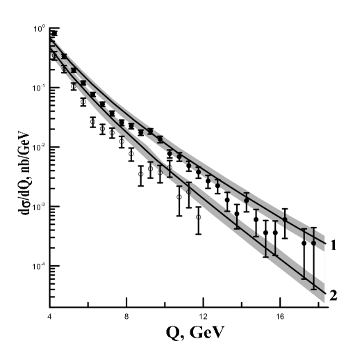
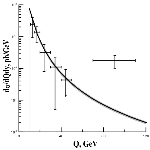
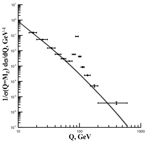
We start our comparison of theoretical predictions with the experimental data for the invariant-mass distributions of the Drell-Yan lepton pairs. In Fig. 1, the predictions of the LO PRA are compared with the data from the R209 Collaboration at the two values of collision energy $\sqrt{S}=44$ GeV and $\sqrt{S}=62$ GeV. The resulting invariant-mass spectrum has been obtained by integration over the relevant virtual photon transverse momentum range and rapidity range $|y|<4$. In Fig. 2, the doubly differential cross section $d\sigma/dQdy$ is presented as function of $Q$ at the $\sqrt{S}=1.8$ TeV, $|y|<1$ and $q_{T}<200$ GeV as it has been measured by CDF Collaboration DY_CDF . In Fig. 3, the data from CMS Collaboration CMSDY are presented as $Q-$spectrum normalized to the cross section in the $Z-$boson peak. The solid line represents our prediction, normalized on the value of cross section in the Z-boson region ($\sigma(60<Q<120\mbox{ GeV})=973$ pb), obtained theoretically in the Ref. CMSDY , see Table 10 therein.

As one would expect, the increase in energy improves an agreement between the theory and experiment. Of course, the $Z-$boson region, $60\leq Q\leq 120$ GeV, is beyond our consideration. An extension of PRA to the region of the $Z-$boson production demands a use of the unknown up today effective vertex $\Gamma^{Z}_{{\cal Q}\bar{\cal Q}}$ which describes the Reggeized quark-antiquark annihilation in $Z-$boson.

To demonstrate an agreement between PRA and Drell-Yan pair spectra over the longitudinal variables, we show in the Fig. 4 the differential cross section $Q^{3}d\sigma/dx_{F}dQ$ as a function of the Feynman variable $x_{F}$ after integration over all $q_{T}$. Curves $1-8$ correspond to $Q$ from $4.75$ GeV till $Q=8.25$ GeV with the step of $0.5$ GeV. The data are from FNAL fixed target experiment FNALXF at the $\sqrt{S}=38.8$ GeV.

Figure 1: Differential cross section of Drell-Yan lepton pair production as function of virtual photon mass $Q$. The data are from R209 Collaboration R209 . The curve 1 – $\sqrt{S}=62$ GeV, the curve 2 – $\sqrt{S}=44$ GeV.

Figure 2: Doubly differential cross section of Drell-Yan lepton pair production as function of virtual photon mass $Q$. The data are from CDF Collaboration DY_CDF at $\sqrt{S}=1.8$ TeV.

Figure 3: Differential cross section of Drell-Yan lepton pair production as function of virtual photon mass $Q$. The data are from CMS Collaboration CMSDY at $\sqrt{S}=7$ TeV. Solid line - our prediction normalized to the theoretical value of the cross-cection in the Z-boson region.

Figure 4: Differential cross section $Q^{3}d\sigma/dx_{F}dQ$ of Drell-Yan lepton pair production as function of $x_{F}$ integrated over all $q_{T}$. Curves $1-8$ correspond $Q$ from $4.75$ GeV till $Q=8.25$ GeV with the step equal to $0.5$ GeV. The data are from FNAL fixed target experiment FNALXF at the $\sqrt{S}=38.8$ GeV.

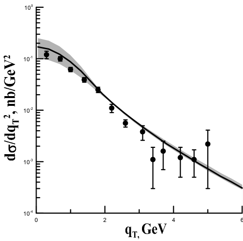
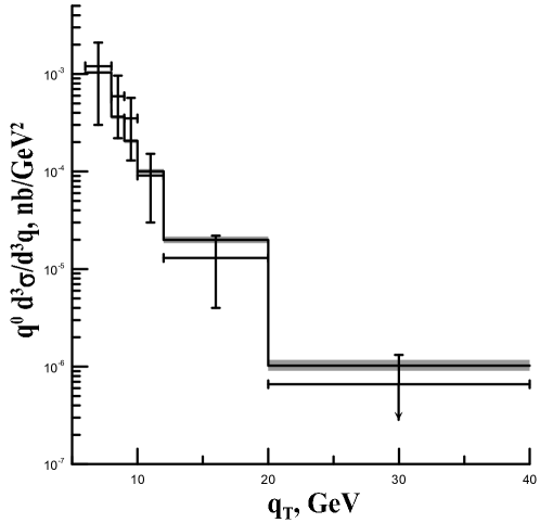
The transverse-momentum dependence of Drell-Yan lepton pair production cross section is demonstrated in Figs. 5 and 6. The R209 Collaboration R209 has measured $q_{T}-$spectrum at $\sqrt{S}=62$ GeV, $|y|<4$, and $5<Q<8$ GeV. We describe this data quite well, especially at small transverse momenta $q_{T}<2$ GeV, where the pure NLO collinear Parton Model calculations break down and where one usually invokes unknown (ad’hoc) nonperturbative intrinsic parton transverse momentum. The scale dependent uncertainties of our calculations are about 20 % and they become larger at $q_{T}<2$ GeV, up to 70 % at the $q_{T}\simeq 0$. However, the average value is still in agreement with experimental data.

The UA1 Collaboration UA1 data for the $q_{T}-$spectrum of Drell-Yan lepton pairs at $\sqrt{S}=630$ GeV are presented as a differential invariant cross section, averaged over the virtual photon mass in the range of $2m_{\mu}<Q<2.5$ GeV, and in the rapidity range $|y|<1.7$. Because the cross section grows steeply when $Q\to 0$ and the lower boundary in $Q$ is fixed at the minimal kinematical value $Q_{min}=2m_{\mu}$ , we need to take into account muon mass $m_{\mu}$ in our calculations. Formally, it boils down to an additional threshold factor $(1-4m_{\mu}^{2}/Q^{2})^{3/2}$ in a formula for the $q_{T}-$spectrum. Taking into account the large experimental error bars, we can conclude that our calculations agree with the data too.

In Fig. 7, we plot our predictions for the transverse-momentum spectra of Drell-Yan lepton pairs at the CERN LHC for energies $\sqrt{S}=7$ and $\sqrt{S}=14$ NeV in two regions of virtual photon masses: $5<Q<50$ GeV, and $120<Q<200$ GeV. The invariant-mass spectra have been obtained after integration over rapidity in the range of $|y|<3$.

Figure 5: Differential cross section of Drell-Yan lepton pair production as function of $q_{T}$. The data are from R209 Collaboration R209 at the $|y|<4$, $5<Q<8$ GeV, $\sqrt{S}=62$ GeV.

Figure 6: Differential cross section of Drell-Yan lepton pair production as function of $q_{T}$. The data are from UA1 Collaboration UA1 at the $|y|<1.7$, $0.2<Q<2.5$ GeV, $\sqrt{S}=630$ GeV.

Figure 7: Differential cross section of Drell-Yan lepton pair production as function of $q_{T}$ at the CERN LHC energy $\sqrt{S}=7$ TeV, and $|y|<3$. Curve 1 - $5<Q<50$ GeV, curve 2 - $120<Q<200$ GeV.

In the next section we compare our theoretical results obtained in the LO PRA with the experimental data for the angular coefficients in Drell-Yan pair production. We consider data from the NuSea Collaboration NuSea at the Tevatron Collider, which correspond to $\sqrt{S}=39$ GeV . We also make prediction for angular coefficients $A_{0},A_{2}$ for CERN LHC at energies $\sqrt{S}=7$ and $\sqrt{S}=14$ TeV.

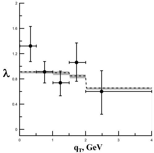
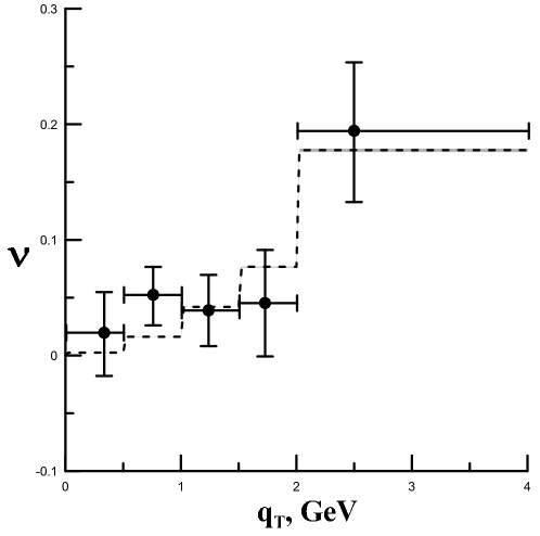
NuSea Collaboration from Fermilab Tevatron recently has published data NuSea for Drell-Yan lepton pair production in fixed-target experiment with hydrogen and deuterium targets and $E_{p}=800$ GeV proton beam ($\sqrt{S}=39$ GeV). The measurements have been done in the following kinematic domain: $4.5<Q<15$ GeV, $0<q_{T}<4$ GeV, $0<x_{F}<0.8$. The results of measurements of angular distributions are presented in terms of angular coefficients $\lambda,\nu,\mu$ as functions of virtual photon transverse momentum. We find good agreement of our LO PRA calculations with data for $\nu$ and $\lambda$ at all values of $q_{T}$, as it is shown in Figs. 8 and 9. Additionally, we predict $\mu=0$ which is also in agreement with the data within the experimental error bars.

Figure 8: Angular coefficient $\nu$ as function of $q_{T}$. The histogram corresponds to LO calculation in PRA with KMR KMR unintegrated PDFs. The data are from NuSea Collaboration NuSea .

Figure 9: Angular coefficient $\lambda$ as function of $q_{T}$. The histogram corresponds to LO calculation in PRA with KMR KMR unintegrated PDFs. The data are from NuSea Collaboration NuSea .

It is known since the works of Lam and Tung LamTungRel , that with allowance for parton subprocesses (3) and (4) in the NLO collinear parton model, one can obtain the relation for the angular coefficients, $A_{0}\simeq A_{2}$. This relation is known to be valid at large $q_{T}$, and it has been verified experimentally in the Z-boson resonance mass region in CDF_A0_A2 . For the region of small dilepton masses it has not been verified yet. As it can be seen from the Figures 10 and 11, in our approach, this relation is approximately valid for energies below 1 TeV and for the large-mass region. For large energies, and especially for the small-mass region (see Fig. 10), this relation is broken at the small values of $q_{T}$. Using the formulas (43), (44),(47) and definitions of angular coefficients (22), one can show that:

$$A_{0}(S,Q^{2},y,q_{T}=0)=\frac{\sum\limits_{q}\int dt\Phi_{q}^{p}(x_{1},t)\Phi_{\bar{q}}^{p}(x_{2},t)\times 4t}{\sum\limits_{q}\int dt\Phi_{q}^{p}(x_{1},t)\Phi_{\bar{q}}^{p}(x_{2},t)\times(Q^{2}+2t)},$$ (54)

$$A_{2}(S,Q^{2},y,q_{T}=0)=0,$$ (55)

where $t=t_{1}=t_{2}$, because of $\vec{q}_{1T}=-\vec{q}_{2T}$ if $\vec{q}_{T}=0$. So, the value of the coefficient $A_{0}$ at the $q_{T}=0$ characterizes the smearing of unintegrated PDF in transverse momentum and it is increasing in the small $x\sim Q_{T}/\sqrt{S}$ region as it shown at the Fig. 10.

Figure 10: Angular coefficients $A_{0}$ (solid curves) and $A_{2}$ (dashed curves) in the proton-proton collisions as functions of $q_{T}$ for the mass region $5<Q<50$ GeV and different center of mass energies. Curves 1,6 – 14 TeV, 2,5 – 7 TeV, 3,4 – 2 TeV.

Figure 11: Angular coefficients $A_{0}$(solid curves) and $A_{2}$(dashed curves) in the proton-proton collisions as functions of $q_{T}$ for the mass region $120<Q<200$ GeV and different center of mass energies. Curves 1,6 – 14 TeV, 2,5 – 7 TeV, 3,4 – 2 TeV.

V Conclusions

We reported a study of the Drell-Yan lepton pair production at LO in the Parton Reggeization Approach, including subprocess (8) with Reggeized quarks in the initial state. The Reggeization allows to account in a simple and compact form the initial and final state radiation effects with full allowance for finite transverse momenta of partons. Our theoretical predictions provide an adequate numerical description of a multitude of the experimental measurements of lepton pair distributions on the invariant mass ($Q$), lepton pair transverse momentum ($q_{T}$) and longitudinal scaling variable ($x_{F}$) as well as lepton pair angular distributions at the SPS, Tevatron and LHC Colliders. This good description is achieved, without any ad-hoc adjustments of input parameters. By contrast, in the collinear Parton Model, such a degree of agreement calls for NLO and NNLO corrections and complementary soft-gluon resummations and ad-hoc nonperturbative transverse momenta of partons. In conclusion, the Parton Raggeization approach has once again proven to be a powerful tool for the theoretical description of QCD processes induced by Reggeized gluons fusion as well as Reggeized quarks annihilation in the high-energy limit.

References

• (1) S.D. Drell and T.M. Yan, Phys. Rev. Lett. 25, 316 (1970).
• (2) NuSea Collaboration, L.Y. Zhu et al. Phys.  Rev.  Lett.  102, 182001 (2009).
• (3) J.P. Ralson and D.E. Soper, Nucl. Phys. B152 (1979) 109.
• (4) M. Anselmino, V. Barone, A. Drago, and N.N.  Nikolaev, Phys. Lett. B594 (2004) 97.
• (5) W.J. Stirling, and M.R. Whalley. J. Phys. G 19, D1 (1993).
• (6) S. Gavin et al. Int. J. Mod. Phys. A 10, 2961 (1995).
• (7) E.L. Berger, J. Qiu, and X. Zhung. Phys. Rev. D 65, 034006 (2002).
• (8) J.C. Collins and D.E. Soper, Nucl. Phys. B 193 (1981) 381; J.C. Collins, D.E. Soper, and G. Sterman. Nucl. Phys. B 250, 199 (1985).
• (9) E.L. Berger, J-W. Qui, and R.A. Rodriguez-Pedraza. Phys. Rev.  D 76, 074006 (2007).
• (10) Yu.L. Dokshitzer, D. Diakonov, and S.I. Troian. Phys. Lett. B 79 (1978) 269-272.
• (11) G. Altarelli, G. Parisi, and R. Petronzio. Phys. Lett. B 76 (1978) 351.
• (12) D. Boer, P.J. Mulders. Nucl.Phys. B569 (2000) 505.
• (13) A. Szczurek, and G. Slipek. Phys. Rev. D 78, 114007 (2008) .
• (14) A.V. Lipatov, M.A. Malyshev, and N.P. Zotov. JHEP 1112, 117 (2011).
• (15) L. N. Lipatov, Nucl. Phys.  B452, 369 (1995).
• (16) L. N. Lipatov, Sov. J. Nucl. Phys.  23, 338 (1976) [Yad. Fiz.  23, 642 (1976)]; E. A. Kuraev, L. N. Lipatov, and V. S. Fadin, Sov. Phys. JETP 44, 443 (1976) [Zh. Eksp. Teor. Fiz.  71, 840 (1976)]; Sov. Phys. JETP 45, 199 (1977) [Zh. Eksp. Teor. Fiz.  72, 377 (1977)]; I. I. Balitsky and L. N. Lipatov, Sov. J. Nucl. Phys.  28, 822 (1978) [Yad. Fiz.  28, 1597 (1978)]; Sov. Phys. JETP 63, 904 (1986) [Zh. Eksp. Teor. Fiz.  90, 1536 (1986)].
• (17) V. S. Fadin and V. E. Sherman, JETP Lett. 23, 599 (1976); JETP 45, 861 (1977).
• (18) V. S. Fadin and L. N. Lipatov, Nucl. Phys.  B406, 259 (1993); B477, 767 (1996).
• (19) V. A. Saleev, Phys. Rev.  D 78, 034033 (2008).
• (20) V. A. Saleev, Phys. Rev.  D 80, 114016 (2009).
• (21) B. A. Kniehl, V. A. Saleev, A. V. Shipilova, E. V. Yatsenko, Phys. Rev.  D84 , 074017 (2011).
• (22) V. A. Saleev, Phys. Rev.  D 78, 114031 (2008).
• (23) F. Hautmann, M. Hentschinski, H. Jung. Preprint IFT-UAM-CSIC-12-39, LPN12-050, OUTP-12-08-P; e-Print: arXiv:1205.1759 [hep-ph].
• (24) CDF Collaboration, A. A. Affolder et all. Phys. Rev. Lett. 84, 845 (2000).
• (25) D0 Collaboration, B. Abbott et all. Phys. Rev. Lett. 82, 4769 (1999) .
• (26) R209 Collaboration, D. Antreassyan et al. Phys. Rev. Lett. 48, 302 (1982).
• (27) UA1 Collaboration, Alitti et al. Phys. Lett. B 275, 202 (1992) .
• (28) LHCb Collaboration, CERN-LHCb-CONF-2012-013.
• (29) CMS Collaboration, S. Chartchuan, JHEP 1110, 007 (2011).
• (30) P. L. Macgauhey et. al., Phys. Rev. D 50, 3038 (1994).
• (31) E. N. Antonov, L. N. Lipatov, E. A. Kuraev, and I. O. Cherednikov, Nucl. Phys.  B721, 111 (2005).
• (32) L. N. Lipatov and M. I. Vyazovsky, Nucl. Phys.  B597, 399 (2001).
• (33) M. Boglione and S. Melis. Phys.  Rev.  D 84, 034038 (2011).
• (34) J.C. Collins, and C.D. Soper. Phys.  Rev.  D 16, 2219 (1977).
• (35) M. A. Kimber, A. D. Martin, and M. G. Ryskin, Eur. Phys. J.  C 12, 655 (2000); Phys. Rev.  D 63, 114027 (2001); G. Watt, A. D. Martin, and M. G. Ryskin, Eur. Phys. J.  C 31, 73 (2003).
• (36) C.S. Lam and W.K. Tung. Phys. Rev. D 18, 2447 (1978).
• (37) C.S. Lam and W.K. Tung. Phys. Lett. B 80, 228 (1979)
• (38) CDF Collaboration, T. Aaltonen et al. Phys. Rev. Lett. 106 241801 (2011)
• (39) G. Watt, A. D. Martin and M. G. Ryskin, Phys. Rev.  D 70, 014012 (2004); 70, 079902(E) (2004).