Driven translocation of a polymer: fluctuations at work

Abstract

The impact of thermal fluctuations on the translocation dynamics of a polymer chain driven through a narrow pore has been investigated theoretically and by means of extensive Molecular-Dynamics (MD) simulation. The theoretical consideration is based on the so-called velocity Langevin (V-Langevin) equation which determines the progress of the translocation in terms of the number of polymer segments, $s(t)$, that have passed through the pore at time $t$ due to a driving force $f$. The formalism is based only on the assumption that, due to thermal fluctuations, the translocation velocity $v=\dot{s}(t)$ is a Gaussian random process as suggested by our MD data. With this in mind we have derived the corresponding Fokker-Planck equation (FPE) which has a nonlinear drift term and diffusion term with a time-dependent diffusion coefficient $D(t)$. Our MD simulation reveals that the driven translocation process follows a superdiffusive law with a running diffusion coefficient $D(t)\propto t^{\gamma}$ where $\gamma<1$. This finding is then used in the numerical solution of the FPE which yields an important result: for comparatively small driving forces fluctuations facilitate the translocation dynamics. As a consequence, the exponent $\alpha$ which describes the scaling of the mean translocation time $\langle\tau\rangle$ with the length $N$ of the polymer, $\langle\tau\rangle\propto N^{\alpha}$ is found to diminish. Thus, taking thermal fluctuations into account, one can explain the systematic discrepancy between theoretically predicted duration of a driven translocation process, considered usually as a deterministic event, and measurements in computer simulations.

In the non-driven case, $f=0$, the translocation is slightly subdiffusive and can be treated within the framework of fractional Brownian motion (fBm).

I Introduction

The polymer translocation through narrow pores is one of the most striking single-molecule experiments motivated mainly by the DNA transport across cell membranes and the possibility of DNA sequencingMeller ; Laan . In nearly two decades of intensive investigations considerable headway has been achieved by a variety of experimental, theoretical and simulational studiesMilchev . In most cases of experimental and simulation studies one deals with a polymer chain that is driven by external electrical field which acts on the monomers passing through the nanopore from the cis- to the trans-side of the separating membrane Meller . Some of the very basic questions one tries to answer concern the time $\tau$ it takes the chain to thread and translocate between the two half-spaces of the setup and in particular, how $\tau$ depends on chain length $N$ and applied force $f$.

The simplest theoretical approach has considered this process as one-dimensional biased diffusion (in terms of the translocated number of segments $s$) over an entropic barrier Sung ; Muthu . Such an approach obviously suffers from some inconsistency since the mean time of the driven translocation $\langle\tau\rangle$ turns to be smaller than the relaxation (Rouse) time of the chain $\tau_{R}$ so that the chain has not enough time to equilibrate and experience the global entropic barrier. Later, it was realized that the chain responds to pulling at first locally in the vicinity of the nanopore with a tensile force spreading away from the separating membrane. This scenario has been treated within the linear response theory (that is, for relatively weak driving forces) and the corresponding memory function has been derived explicitly Panja_1 ; Panja_2 . For arbitrary strong driving forces, an interesting approach based on the notion of tensile force propagation along the chain backbone has been suggested by Sakaue Sakaue_1 ; Sakaue_2 ; Sakaue_3 . Sakaue’s idea has been used and worked out very recently in other theoretical treatments Dubbeldam_1 ; Ikonen .

Despite increased insight in the nature of the translocation process, however, current understanding of the translocation dynamics is still far from satisfactory. So, among other things, there exists a non-negligible systematic discrepancy between the theoretical (analytical) predictions concerning the main scaling exponents that characterize translocation dynamics and the data provided by computer experiments, mainly Molecular Dynamics (MD) simulation studies Milchev .

Recently Dubbeldam_1 we suggested a theoretical description based on the tensile (Pincus) blob picture of a pulled chain and the notion of a tensile force propagation, introduced by Sakaue Sakaue_1 ; Sakaue_2 ; Sakaue_3 . Assuming that the local driving force is matched by a drag force of equal magnitude, (i.e., in a quasi-static approximation), we derived an equation of motion for the tensile front position. This enables one to calculate the deterministic dependence (i.e., without taking into account fluctuations) of the translocation coordinate as a function of time $M(t)$. One can obtain the scaling law for the mean translocation time $\langle\tau\rangle$ vs. chain length $N$, i.e., $\langle\tau\rangle\propto N^{\alpha}$, where $\alpha$ is the translocation exponent. The total translocation process consists of two stages. First, the tensile force propagates so that more and more polymer segments get involved in the moving domain. Depending on the driving force $f$, which is applied to the segment in the pore, the moving domain attains different shapes: “trumpet”, “stem-trumpet”, or a “stem”, for weak, intermediate and strong forces, respectively. Once the last polymer segment on the cis-side of the pore gets involved, the velocity of the moving domain approaches a stationary value. After that the second stationary stage sets in and the rest of the chain is sucked into the pore with constant velocity.

We have shown Dubbeldam_1 that for the “trumpet” case, the characteristic duration (in the case of Rouse dynamics) of the first and second stages goes as $\tau_{1}\propto N^{1+\nu}/f$ and $\tau_{2}\propto N^{2\nu}/f^{1/\nu}$ respectively (where $\nu\approx 3/5$ is the Flory exponent), so that at ${\tilde{f}}_{R}\stackrel{{\scriptstyle\rm def}}{{=}}aN^{\nu}f/k_{B}T\gg 1$ the first stage time dominates. As a consequence, with growing chain length $N$ and force $f$, the translocation exponent $\alpha$ also increases from $\alpha=2\nu\approx 1.19$ to $\alpha=1+\nu\approx 1.59$. These predictions are supported by our simulation findings Dubbeldam_1 as well as by results of Lehtola et al. Lehtola_1 ; Lehtola_2 ; Lehtola_3 but differ from the results of Luo et al. Luo . The tensile force propagation phenomenon treated within the iso-flux trumpet model also leads to $\alpha=1+\nu$ Grosberg .

Unfortunately, the MD-simulation results yield systematically smaller values for the translocation exponent $\alpha$. For example, in our MD-simulations $\alpha\approx 1.33$ for strong forces and $\alpha\approx 1.06$ for weak forces (distinct from the theoretical predictions $\alpha=1+\nu\approx 1.59$, and $\alpha=2\nu\approx 1.18$ respectively). It is important to determine the origin of this inconsistency since apparently there is something missing in the afore mentioned theoretical consideration which gives room for speculations. For example, in a paper by Ikonen et at. Ikonen , the model based on the idea of tensile force propagation Sakaue_1 ; Sakaue_2 ; Sakaue_3 and the role of pore-polymer friction has been numerically investigated. The authors argue that the theoretical value for the exponent, $\alpha=1+\nu$, may be seen only for very long chains whereas for the chain lengths used in real experiments or simulations the effective exponent $\alpha$ could be approximately 20% smaller.

In this work we consider theoretically and by means of MD-simulations how fluctuations of the translocation coordinate (such fluctuations have been ignored in the quasi-static approximation as in the other deterministic treatments) affect the forced translocation dynamics. Indeed, the role of thermal fluctuations is by no means self-evident. A recent publication Sakaue_4 argues that only fluctuations related to the initial distribution of segments are essential whereas thermal fluctuations have a minor effect. Moreover, the authors argue Sakaue_4 that the translocation exponents are not affected by the fluctuations in the initial conditions.

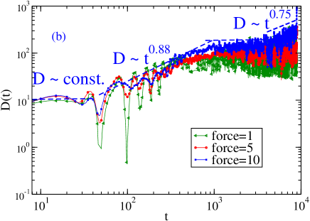
In the present investigations we demonstrate that thermal fluctuations may facilitate the translocation dynamics so that the effective translocation exponent $\alpha$ becomes smaller. To this end in Section II we derive a Fokker-Planck equation (FPE) for the translocation coordinate $s$ probability distribution function $W(s,t)$. This FPE, which contains a nonlinear drift term and a time-dependent diffusion coefficient $D(t)$, is then solved numerically demonstrating a significant fluctuation-induced facilitation of the translocation dynamics. In Section III we then present our simulation results. First, we prove that the translocation velocity under differently strong driving forces is a random process with a Gaussian distribution which is the only conjecture we need for our theory. Then we calculate the velocity autocorrelation function (VAF) which reveals an oscillatory behavior and a long-time tail. This gives rise to a time-dependent diffusion coefficient $D(t)\propto t^{\gamma}$, where the exponent $\gamma<1$, indicating a super-diffusively driven translocation. We end this report with a brief summary of conclusions in Section IV. Some technical details relegated to the Appendices A, B.

II From Langevin to Fokker-Planck equation

In order to allow for fluctuations of the translocation coordinate one should consider the problem within the framework of the corresponding Fokker-Planck (FPE) equation which governs the probability distribution function (PDF) $W(s,t)$ that exactly $s$ segments have passed the pore at time $t$. By so doing we follow our earlier approach ref. Dubbeldam_2 where the case of undriven translocation was treated. We focus here on the general case when the drift term in FP-equation is essential

Our approach is based on the assumption that the translocation coordinate $s(t)$, which measures the number of segments heaving reached the trans-side at time $t$, is a random process governed by the so-called V-Langevin (where V stands for “velocity”) equation

$$\dfrac{ds(t)}{dt}=v\left(s(t)\right)$$ (1)

This equation has been discussed extensively by Balescu Balescu mainly in the context of plasma dynamics. The translocation velocity $v\left(s(t)\right)$ in Eq. (1), which depends on the trajectory $s(t)$, is assumed to be a Gaussian process with given first moment

$$\left\langle v(s(t))\right\rangle\stackrel{{\scriptstyle\rm def}}{{=}}\left.K(s)\right|_{s=s(t)}\stackrel{{\scriptstyle\rm def}}{{=}}-\dfrac{1}{\xi_{0}}\left.U^{\prime}(s)\right|_{s=s(t)}$$ (2)

and a two-point correlation function

$$\left\langle\left[v(s(t_{1}))-\langle v(s(t_{1}))\rangle\right]\left[v(s(t_{2}))-\langle v(s(t_{2}))\rangle\right]\right\rangle\stackrel{{\scriptstyle\rm def}}{{=}}G(t_{1},t_{2})$$ (3)

.

In Eq. (2) the function $U(s)$ stands for the effective potential in the translocation coordinate space $s$ while $\xi_{0}$ is the corresponding friction coefficient. The form of the averaged velocity $K(s)$ as well as the effective potential $U(s)$ we will find below using the correspondence principle. This principle states that in the limit of very small fluctuations the FPE solution reproduces the deterministic (or quasi-static) solution $\left\langle s(t)\right\rangle=M(t)$ which was derived in ref. Dubbeldam_1 . The case of colored Gaussian statistics as well as the behavior of the VAF $G(t_{1},t_{2})$ will be studied by MD-simulation in Sec. III. This will be considered as the required dynamic input while solving the corresponding FPE.

Based on the V-Langevin Eq. (1), one could derive the corresponding FPE for the PDF $W(s,t)$. The latter is defined as follows

$$W(s,t)=\langle\delta(s-s(t))\rangle$$ (4)

where $\langle\dots\rangle$ means an average over the Gaussian velocity field fluctuations with a first moment and two-point correlation function given by Eq. (2) and Eq. (3), respectively. The detailed derivation is given in Appendix A. The resulting FPE reads

$$\dfrac{\partial W(s,t)}{\partial t}=-\dfrac{\partial}{\partial s}[K(s)W(s,t)]+{D(t)}\>\dfrac{\partial^{2}}{\partial s^{2}}\>W(s,t)$$ (5)

where the time dependent diffusion coefficient

$$D(t)=\int_{0}^{t}G(t,\tau)d\tau.$$ (6)

It should be stressed that Eq. (5) is rather general. Indeed, no assumptions regarding, for example, the validity of the fluctuation-dissipation theorem are made in the course of derivation in contrast to the case of the generalized Langevin equation approach Cherail ; Panja . Moreover, the drift and diffusion terms are totally independent (i.e. the Stokes-Einstein relation does not necessarily hold). In other words, this FPE is valid even for a highly non-equilibrium driven translocation processes.

II.1 What is the form of $K(s)$?

As mentioned above, the form of $K(s)$ can be fixed by making use of the correspondence principle which states that in the limit of zero fluctuations the FPE reproduces the deterministic solution for the first moment, $\left\langle s(t)\right\rangle=M(t)$, derived in ref. Dubbeldam_1 , i.e.

$$M(t)=\left(c_{0}{\widetilde{f}}_{a}{\widetilde{t}}\right)^{\beta}$$ (7)

where the dimensionless force ${\widetilde{f}}_{a}=af/T$ and time ${\widetilde{t}}=t/\tau_{0}$ with $a$, $T$ and $\tau_{0}=a^{2}\xi_{0}/T$ standing for the Kuhn segment length, temperature, and the microscopic characteristic time, respectively. In Eq. (7) $c_{0}$ is a constant of the order of unity and the exponent $\beta$ in the limit of strong driving forces reads $\beta=1/(1+\nu)$ Dubbeldam_1 .

In this limit $G(t,\tau)=0$, $D(t)=0$ and Eq. (5) reduces to

$$\dfrac{\partial W(s,t)}{\partial t}=-\dfrac{\partial}{\partial s}[K(s)W(s,t)]$$ (8)

On the other hand, in this case $W(s,t)=\delta(s-M(t))$ and Eq. (8) is equivalent to

$$\dfrac{\partial}{\partial t}\delta(s-M(t)) = -K(M(t))\;\dfrac{\partial}{\partial s}\>\delta(s-M(t))$$ (9)

$$= -{\dot{M}}\>\dfrac{\partial}{\partial s}\>\delta(s-M(t))$$

where in the first line we have used that $K(s)\delta(s-M(t))=K(M(t))\delta(s-M(t))$, and in the second line the chain rule has been used. As a result the FPE is equivalent to the deterministic equation

$$\dfrac{d}{dt}M(t)=K(M(t))$$ (10)

It is easy to show that in order to restore the solution, Eq. (7), the function $K(s)$ in Eq. (10) should be of the form

$$K(s)=\dfrac{\beta c_{0}f}{a\xi_{0}}\>s^{-(1-\beta)/\beta}$$ (11)

It is also instructive to reconstruct the form of the effective potential $U(s)$, given by Eq. (2). Namely, from Eq. (2) and Eq. (11) one has $U^{\prime}(s)=-(\beta c_{0}f/a)\>s^{-(1-\beta)/\beta}$. As a result, the effective potential that governs the translocation reads

$$U(s)=U_{0}-\dfrac{\beta c_{0}f}{a(2-1/\beta)}\>s^{2-1/\beta}$$ (12)

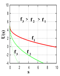
i.e., it has the form of the slanting plane shown in Fig. 1.

Figure 1: Effective potential $U(s)$ ( given by Eq.( 12)) as a function of the translocation coordinate $s$ at different forces: $f_{3}>f_{2}>f_{1}$.

II.2 Two ways to calculate $D(t)$ by using MD-data

The behavior of the diffusion coefficient $D(t)$ which is necessary as an input for the solution of the FPE, could be found using a MD-simulation by two methods. First, one could directly calculate the VAF $G(t,\tau)$ and then integrate it over the time according to Eq. (6). On the other hand, there is a simple relationship between the time dependent variance $\left\langle\Delta s^{2}(t)\right\rangle\stackrel{{\scriptstyle\rm def}}{{=}}\langle[s(t)-\langle s(t)\rangle]^{2}\rangle$ and $D(t)$. Indeed, first of all $s(t)=s_{0}+\int_{0}^{t}v(s(t_{1}))dt_{1}$ , i.e. $\langle s(t)\rangle=s_{0}+\int_{0}^{t}\langle v(s(t_{2}))\rangle dt_{2}$. Thus,

$$\left\langle[s(t)-\langle s(t)\rangle]^{2}\right\rangle = \int_{0}^{t}dt_{1}\int_{0}^{t}dt_{2}\left\langle\delta v(s(t_{1}))\delta v(s(t_{2}))\right\rangle$$ (13)

$$= \int_{0}^{t}dt_{1}\int_{0}^{t}dt_{2}\>G(t_{1},t_{2})$$

where, as before, $\delta v(s(t))=v(s(t))-\langle v(s(t))\rangle$. Finally, differentiation of $\left\langle\Delta s^{2}(t)\right\rangle\stackrel{{\scriptstyle\rm def}}{{=}}\langle[s(t)-\langle s(t)\rangle]^{2}\rangle$ in Eq. (13) leads to

$$\dfrac{d\left\langle\Delta s^{2}(t)\right\rangle}{2dt}=\int_{0}^{t}\>G(t,\tau)d\tau=D(t)$$ (14)

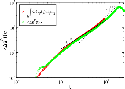
where we have used that $G(t_{1},t_{2})=G(t_{2},t_{1})$. In Section III we will show that the mean squared displacement $\left\langle\Delta s^{2}(t)\right\rangle$, calculated by the double integration of the VAF (see Eq. (13)) over time, and by the direct simulation, gives closely matching results.

II.3 Numerical Solution of the FP-equation

The FPE, Eq. (5), can be easily solved numerically assuming reflection-adsorption boundary conditions and some reasonable guess about the form of time-dependent diffusion coefficient $D(t)$. The direct inspection of simulation data, given in Sec. III.2, shows that the VAF $G(t_{1},t_{2})$ has a long-time tail, i.e., correlations persist in time. This, according to Eq. (14), leads to a time-dependent diffusion coefficient $D(t)$ which could be approximated by a power law

$$D(t)=\dfrac{d_{0}}{\tau_{0}}\>{\tilde{t}}^{\gamma}$$ (15)

where $d_{0}$ is a constant and the exponent $\gamma<1$. Before we proceed further with the results of numerical solution, let us give a short discussion of the small-noise expansion of the FPE, Eq. (5), where the diffusion coefficient is a small time-dependent function, i.e., $D(t)=(\varepsilon^{2}/2)D_{0}(t)$, with $D_{0}(t)\propto{\tilde{t}}^{\gamma}$. Following the book of Gardiner Gardiner , in the Appendix B we give a more extensive discussion of the small-noise expansion around the deterministic solution. In particular, for the first moment this expansion yields

$$\left\langle s(t)\right\rangle=\left(c_{0}{\tilde{f}}{\tilde{t}}\right)^{\beta}+\dfrac{\varepsilon^{2}{\tilde{d}_{0}}}{{\tilde{f}}^{\beta}}\>{\tilde{t}}^{1+\gamma-\beta}$$ (16)

As is evident from Eq. (16), the fluctuations are responsible for speeding of the translocation process. The corresponding fluctuation increment is of the $\varepsilon^{2}$-order (the same as the diffusion coefficient, $D(t)=\varepsilon^{2}D_{0}(t)/2$, itself) and goes with time as $t^{1+\gamma-\beta}$. In order to estimate the exponent $1+\gamma-\beta$, one needs the exponent $\gamma$. One could use the data for $\left\langle\Delta s^{2}(t)\right\rangle$, given by Bhattacharya et al. Bhattacharya where it was reported that $\left\langle\Delta s^{2}(t)\right\rangle\sim t^{1.44}$. As a result, according to Eq. (14), the (reduced) diffusion coefficient $D_{0}(t)\sim t^{0.44}$, i.e. $\gamma=0.44$. This estimate leads (taking also into account that $\beta=1/(1+\nu)\approx 0.63$) to the behavior of fluctuation increment $\sim t^{0.81}$ which facilitates the translocation dynamics as $\left\langle s(t)\right\rangle=(c_{0}{\tilde{f}}{\tilde{t}})^{0.63}+(\varepsilon^{2}{\tilde{d}_{0}}/{\tilde{f}}^{0.63})\>{\tilde{t}}^{0.81}$. In the general case, an effective exponent enhancement is possible, if at least $1+\gamma-\beta>\beta$, i.e.,

$$\gamma>2\beta-1$$ (17)

Thus, there is a lower limit for the $\gamma$ value which ensures the effective exponent (in the $\langle s(t)\rangle$ vs. $t$ dependence) enhancement. For example, if $\beta=1/(1+\nu)$ then $\gamma>(1-\nu)/(1+\nu)\approx 0.26$.

The relationship, Eq. (17), can be also readily obtained by the following arguments. If $\langle\Delta s^{2}\rangle\propto t^{\theta}$, then the first two moments could be estimated as $\langle s\rangle\propto t^{\theta/2}$ and $\langle s^{2}\rangle\propto t^{\theta}$. But in the case of quasi-static (no fluctuations) approximation $\langle s\rangle\propto t^{\beta}$ and, provided that $\theta/2>\beta$, some slope enhancement owing to fluctuations takes place. Taking into account that according to Eq. (14 ) $\theta=\gamma+1$, one immediately arrives at Eq. (17).

Figure 2: The result of numerical solution of Eq. (5) for two different driving forces, $f=1$ (lower curves), $f=10$ (upper curves), and exponents $\gamma=0,0.4,0.8$. The dashed line corresponds to the quasi-static approximation with a slope $\beta=1/(1+\nu)\approx 0.63$. Taking into account fluctuations with $D(t)\propto t^{0.8}$ leads to a slope (or, an effective exponent) enhancement up to $0.75$. The chain length $N=100$.

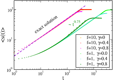
Figure 2 demonstrates the numerical solution of the FPE, Eq. (5), for the first statistical moment, $\langle s(t)\rangle$, as a function of time (the chain length $N=100$). It can be seen that for a relatively strong force

Figure 3: (a) The PDF function $W(s,t)$ for $f=1$, $\gamma=0.4$ and (inset) the corresponding statistical moments $\langle s(t)\rangle$, $\langle s^{2}(t)\rangle$, $\langle\Delta s^{2}(t)\rangle$ . (b) The same but for the exponent $\gamma=0$.

(upper set of curves for $f=10$), the fluctuation has little or no effect on the $\langle s(t)\rangle$ behavior. For weaker force, e.g., for $f=1$, shown by the lower set of curves, and relatively large exponent $\gamma=0.8$, one can see a clear slope enhancement, up to $0.75$. Thus, one may argue that under relatively small driving forces fluctuations facilitate the translocation dynamics.

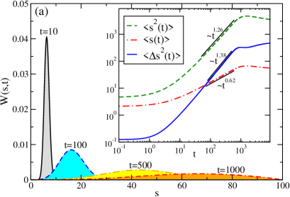
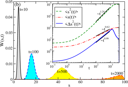
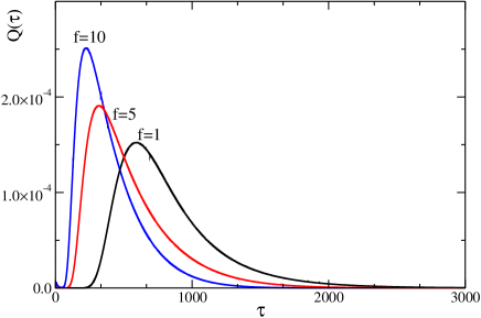
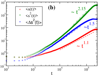
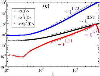
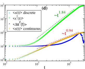
The results of numerical solution for the PDF $W(s,t)$ as well as the corresponding statistical moments, $\langle s(t)\rangle$ , $\langle s^{2}(t)\rangle$, $\langle\Delta s^{2}(t)\rangle$, are shown in Fig. 3 for different parameters. As one might expect, the time dependence of the variance follows the law $\langle\Delta s^{2}(t)\rangle\propto t^{\theta}$, where the exponent $\theta=\gamma+1$ in accordance with Eq. (14). In other words, for the running diffusion coefficient, $D(t)\propto t^{\gamma}$, with $\gamma<1$, the exponent $1<\theta<2$ and one finds a case of superdiffusion. It is of interest that, due to the external force (in this case $f=1$) and the adsorption boundary condition ($W(s=N,t)=0$), the PDF $W(s,t)$ becomes narrower at a later stage of the translocation. This results in a non-monotonic behavior of the variance $\langle\Delta s^{2}(t)\rangle$ for $\gamma=0.4$, and especially for $\gamma=0$ (see Fig. 3). These numerical findings for the statistical moments are qualitatively consistent with our MD-results given in Fig. 6. Eventually, the first passage time probability distribution (FPTD), $Q(t)=-(d/dt)\int_{0}^{N}\>W(s,t)ds$, for different forces ($f=1,5,10$) is depicted in Fig. 4.

Figure 4: The first-passage time distributions (FPTD) $Q(t)$ calculated for $\gamma=0.4$ and different forces $f=1,5,10$.

II.4 Continuous Time Random Walks (CTRW) approach and beyond

It is pertinent to note that the interpretation of the superdiffusion in terms of the time persistent correlations in the VAF and the time-dependent diffusion coefficient goes actually beyond the polymer translocation problem. Recall that there are two reasons for the occurrence of an anomalous diffusion Bouchaud : i) The consecutive steps of a random walker are independent but the waiting time distribution is a sufficiently broad function, $\psi(t)\sim 1/t^{1+\mu}$, where $\mu<1$, so that the first statistical moment does not exist. ii) There is a long-time correlation between random steps. In the first case, the diffusion process could be rationalized in terms of a continuous-time random walks (CTRW) approach which finally leads to a subdiffusive behavior Sokolov ; KM . The anomalous diffusion in an external force could be quantified in terms of the fractional FP-equation (FFPE)Sokolov ; KM . Later, this FFPE formalism has been applied to the driven polymer translocation problem with an external potential approximated by a function linear in $s$, that is, $U(s)=U_{0}-fs$ Biophys_Journal ; Dubbeldam_3 . Apparently, this approach does not take into account the tensile force propagation and the moving domain reflecting the chain reaction which were discussed above (see e.g. the resulting effective nonlinear potential Eq. (12) ). The calculations within the FFPE formalism suggest that to a leading order $\langle s\rangle\propto t^{\mu}$ and $\langle s^{2}\rangle\propto t^{2\mu}$ i.e. the variance goes superdiffusively, $\langle\Delta s^{2}\rangle\propto t^{2\mu}$, because $1<2\mu<2$ Dubbeldam_3 .

Our simulation results make it clear (see Sec. III.2 and Fig. 7a) that in the case of translocation dynamics correlations persist in time and the CTRW-approach presumably could not be used. In contrast, the formalism of the V-Langevin equation, used in this Section, gives a general way to treat the anomalous diffusion. This approach corresponds closely to driven dynamics because neither the fluctuation-dissipation theorem or the Stokes-Einstein relation, nor time-translation invariance of the correlation functions appears to hold in this case.

III Simulation Results

III.1 Model

In order to verify that the assumptions made in the theoretical analysis are justified, we performed a number of simulations of polymer chains threading through a nanopore. We used MD simulations as in Ref. Dubbeldam_2 . Here we briefly recapitulate the used algorithm.

The model we used describes Langevin dynamics of a polymer chain which consists of $N$ beads that thread through an octagonal pore in a closely-packed wall (membrane). The interaction between the monomers of the chain is modeled by a Finitely Extensible Nonlinear Elastic (FENE) springs corresponding to a pair potential

$$U_{FENE}(r_{ij}) =-\frac{kr_{ij}^{2}}{2}\ln\left(1-\frac{r_{ij}^{2}}{R_{0}^{2}}\right),$$ (18)

where $r_{ij}$ is the bond length between two beads and $R_{0}=1.5$ is the maximal bond length. All beads experience excluded volume interactions which are modeled by the repulsive part of the shifted Lennard-Jones potential, also known as the Weeks-Chandler-Andersen (WCA) potential. This potential $U_{WCA}$ is defined by

$$U_{WCA}(r_{ij})=4\epsilon\left[\left(\frac{\sigma}{r_{ij}}\right)^{12}-\left(\frac{\sigma}{r_{ij}}\right)^{6}+\frac{1}{4}\right]\Theta(r_{c}-r),$$ (19)

where $\Theta(x)$ is the Heaviside-function, i.e., we use a cut-off $r_{c}=2^{-1/6}\sigma$, implying $U_{WCA}=0$ for $r_{ij}>r_{c}$. The monomers residing inside the pore experience a constant external force $f$ in the direction perpendicular to the membrane, which we designate by $x$. The external force can be implemented by adding a linear potential $U_{ext}$, whose value is $0$ outside the pore and $fx$, if $x$ is inside the pore region. Thus, $f$ pulls the chain towards the region of positive $x$ which we refer to as the trans-side. The equation of motion for the beads of the chain reads

$$m\frac{d^{2}\bf{r}_{i}}{dt^{2}}=-\nabla\left(U_{FENE}+U_{LJ}+U_{ext}\right)-\gamma\frac{d{\bf r}_{i}}{dt}+{\cal R}_{i}(t),$$ (20)

where ${\cal R}_{i}(t)$ stands for a Brownian random force whose moments obey $\langle{\cal R}_{i}(t)\rangle=0$ and $\langle{\cal R}_{i}^{\alpha}(t_{1}){\cal R}_{j}^{\beta}(t_{2})\rangle=2k_{B}T\gamma\delta(t_{1}-t_{2})\delta_{\alpha,\beta}\delta_{i,j}$ The parameter values were set to $\epsilon=1.0$, $\sigma=1.0$, $k=60.0$, $\gamma=0.70$ and were kept fixed during the simulations. The temperature had a constant value given by $T=1.20\epsilon/k_{B}$.

The membrane is modeled by a plane of beads whose positions are kept fixed. Eight neighboring monomers are removed to obtain an octagonal pore. The interaction between the beads of the chain and the plane is mediated through the repulsive WCA potential. All simulations were performed starting from a configuration in which initially the chain is placed such that all but one monomer reside on the cis-side. In order to prevent the chain from escaping to the trans-side, we impose reflecting boundary conditions on the first monomer. The chain is fully translocated when all beads have made their way to the trans side.

III.2 Results

Figure 5: The velocity distribution, $P(v_{z})$, for two different forces, (a) $f=0$, (b) $f=1$, and three different time moments. Solid lines represent the Gaussian distribution fitting.

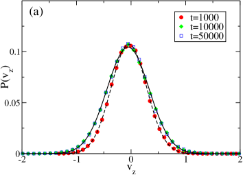
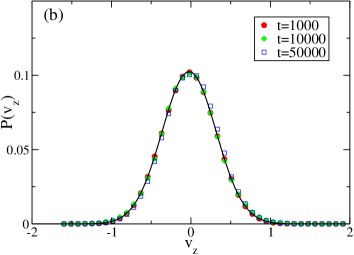
First of all we need to prove that the translocation velocity follows indeed a Gaussian distribution. Simulations were performed for a chain length $N=100$ in the case of free ($f=0$) and driven ($f=1$) translocation. We have approximated the translocation velocity, $v(t)=ds(t)/dt$, by $v_{z}(t)$ , the $z$-component of the Cartesian velocity of the bead inside the pore Dubbeldam_2 . Then we recorded data of the velocity at specific time moments and made histograms over $4000$ runs. As can be seen from Fig. 5, the velocity corresponds closely to a Gaussian distribution (solid lines). This justifies our basic assumption, used in the derivation of the FPE, see Section II.

The statistical moments of the translocation coordinate which are plotted in Fig. 6 for different forces, also provide an important information. While in the unbiased translocation case, Fig. 6a, the diffusion is Brownian (or slightly subdiffusive Dubbeldam_2 ), in the biased regime the process becomes superdiffusive, i.e., the variance $\langle\Delta s^{2}\rangle\propto t^{\theta}$ where $1<\theta<2$. Moreover, the exponent $\theta$ increases with the growth of the driving force $f$, namely, $\theta=1.5$ for $f=1$ (see Fig. 6b), and $\theta=1.84$ for $f=10$ (see Fig. 6d). For relatively large forces ($f=5,10$), the variance $\langle\Delta s^{2}\rangle$ is nonmonotonic, i.e., it goes through a maximum at a late stage of the translocation. This finding is in agreement with our results of the FPE numerical solution given in Sec. II.3 (see Fig. 3).

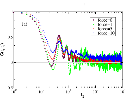
The superdiffusive behavior for $\langle\Delta s^{2}\rangle$ implies (according to the relationship Eq. (14) ) that the diffusion coefficient is a growing function of time which has been approximated by a power law, Eq. (15), in Section II.3. On the other hand, in accordance with Eq. (6), the time-dependent diffusion coefficient $D(t)$ can be obtained by integration of the VAF $G(t_{1},t_{2})$. In Fig. 7a we display the normalized VAF $G(t_{1},t_{2})/G(t_{1},t_{1})$ for $t_{1}=0$ as a function of $t_{2}$. This figure indicates that the VAF has a fairly complex behavior: it changes sign and reveals a long-time tail. It can also be seen that stronger forces imply longer time correlations which give rise to the observed superdiffusive behavior. All measurements have been averaged over $5000$ runs (except for $f=1$ which was obtained by averaging over only $400$ runs).

Figure 6: The first $\langle s\rangle$ and second $\langle s^{2}\rangle$ moments as well as the variance $\langle\Delta s^{2}(t)\rangle=\langle s^{2}\rangle-\langle s\rangle^{2}$ for chain length $N=100$ and different driving forces $f$: (a) $f=0$. (b) $f=1.0$, (c) $f=5.0$. (d) $f=10.0$.

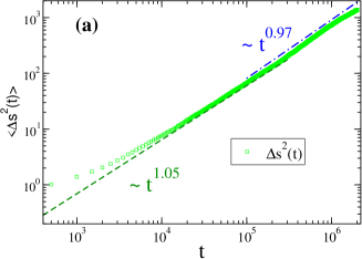
The corresponding diffusion coefficient $D(t)$ could be obtained by simple integration over time, according to Eq. (6). The result of this calculation, given in Fig. 7b, shows that the exponent $\gamma$ attains different values within different time intervals. Eventually, we perform a consistency check. On the one hand, we integrate the expression for $G(t_{1},t_{2})$ over time arguments which provides, according to Eq. (13), the value of $\langle\Delta s^{2}(t)\rangle=\int_{0}^{t}dt_{1}\int_{0}^{t}dt_{2}G(t_{1},t_{2})$. On the other hand, the MD-simulation yields the direct time dependence $\langle\Delta s^{2}(t)\rangle$. This comparison of two different calculations of $\langle\Delta s^{2}(t)\rangle$, displayed in Fig. 8, gives almost identical results for $f=10$.

Figure 7: (a) The velocity autocorrelation function for four different values of force. The stronger forces trigger a longer in time correlations. The vertical axis is normalized by $G(t_{1},t_{1})$. (b) The diffusion coefficient $D(t)$ as function of time. Larger diffusion coefficients arise with $f$ increases.

Figure 8: The value of $\langle s^{2}(t)\rangle$ calculated by two different ways: by integrating the VAF $G(t_{1},t_{2})$ over time, i.e. $\langle\Delta s^{2}(t)\rangle=\int_{0}^{t}dt_{1}\int_{0}^{t}dt_{2}G(t_{1},t_{2})$, and by direct simulation. Chain length $N=100$, force $f=10$.

IV Conclusion

We have investigated theoretically as well as by extensive MD-simulation the role of fluctuations for the case of driven polymer translocation through a nanopore. The consideration is based on the V-Langevin equation, Eq. (1) where the velocity is a random process with Gaussian distribution. Keeping this in mind we have derived a corresponding FPE, Eq. (5), with a nonlinear drift-term and time-dependent diffusion coefficient $D(t)$ which can be represented as time integral of VAF $G(t_{1},t_{2})$ (see Eq. (6)). The derivation requires neither the validity of the fluctuation-dissipation theorem (as in case of the generalized Langevin equation approach Cherail ) nor the time-translation invariance of $G(t_{1},t_{2})$. Such a general approach becomes an important tool for the description of driven translocation dynamics.

It is pertinent to note two limiting cases. In the zero-fluctuation limit, e.g., when the driving force is large, one recovers the deterministic solution. For example, for the first moment it is given by Eq. (7)) which we have discussed recently Dubbeldam_1 . In the zero-force case (nondriven translocation), in contrast, Eq.(5) leads to the fractional Brownian motion (fBm) description which was treated in our previous paper Dubbeldam_2 . The fact that $D(t)$ is a growing function of time (see Eq. (15)), implies that VAF $G(t_{1},t_{2})$ has a long-time tail (long persistence of correlations). This has been verified by our MD-simulation results (see Fig. 7a and Fig. 7b ). By making use the MD-simulation we have also checked the Gaussian distribution of the translocation velocity (see Fig. 5).

The numerical solution of the resulting FPE, Eq. (5), reveals a number of salient features. If the exponent $\gamma$ governing the time dependence of the diffusion coefficient, $D(t)\propto t^{\gamma}$ , is large enough (see the condition given by Eq. (17) ), fluctuations “assist“ the translocation dynamics and the translocation coordinate $\langle s\rangle\propto t^{\beta}$ dependence becomes steeper. Moreover, the variance follows the law $\langle\Delta s^{2}\rangle\propto~{}t^{\theta}$, where the exponent $1<\theta<2$, i.e., the dynamics is superdiffusive. The increase in slope due to fluctuations could, therefore, explain the systematic disagreement between deterministic theory and the MD-simulation results which has been discussed in ref. Dubbeldam_1 . One should recall that the scaling law for the mean translocation time reads $\langle\tau\rangle\propto N^{\alpha}$ where $\alpha\approx 1/\beta$. Owing to fluctuations, $\beta$ grows so that the translocation exponent $\alpha$ becomes smaller in agreement with the MD-simulation.

Appendix A Derivation of the Fokker-Planck-Equation (FPE)

Differentiation of Eq. (4) with respect to $t$ and using the chain rule and the property of the $\delta$-function yields

$$\dfrac{\partial W(s,t)}{\partial t} = -\dfrac{\partial}{\partial s}\left\langle\dfrac{ds(t)}{dt}\delta(s-s(t))\right\rangle$$ (21)

$$= -\dfrac{\partial}{\partial s}\left\langle v\left(s(t)\right)\delta(s-s(t))\right\rangle$$

where the differential operator $\partial/\partial s$ can be put out of averaging because the $\delta$-function is the only one which depends on $s$. In Eq. (21) we have used the Langevin equation Eq. (1). By making use the relation $\langle v(s(t))\rangle\delta(s-s(t))=\langle v(s)\rangle\delta(s-s(t))$, Eq. (21) can be written as

$$\dfrac{\partial W(s,t)}{\partial t}=-\dfrac{\partial}{\partial s}K(s)\left\langle\delta(s-s(t))\right\rangle-\dfrac{\partial}{\partial s}\left\langle\delta v(s(t))\delta(s-s(t))\right\rangle$$ (22)

where $\delta v(s(t))\stackrel{{\scriptstyle\rm def}}{{=}}v(s(t))-\langle v(s(t))\rangle$ and we have used Eq. (2). The second term in Eq. (22) could be expressed in terms of $W(s,t)$ by employing Novikov’s theorem Novikov ; Zinn-Justin . According to Novikov’s theorem, if $g(t)$ is a colored Gaussian random process with a zero average, i.e., $\langle g(t)\rangle=0$, and the two-point correlation function is given by $\langle g(t_{1})g(t_{2})\rangle=G(t_{1},t_{2})$, then for an arbitrary functional, ${\cal R}\{g(t)\}$, the average $\left\langle g(t){\cal R}\{g(t)\}\right\rangle$ can be written as

$$\left\langle g(t){\cal R}\{g(t)\}\right\rangle=\int\limits_{0}^{t}\>d\tau G(t,\tau)\left\langle\dfrac{\delta{\cal R}\{g(t)\}}{\delta g(\tau)}\right\rangle$$ (23)

where the symbol $\delta/\delta g(\tau)$ stands for a functional derivative.

Let’s use now the Novikov’s theorem to recast the second term in the r.h.s of Eq. (22). In this case $g(t)=\delta v(s(t))$ and ${\cal R}\{g(t)\}=\delta(s-s(t))$. As a result, Eq. (22) takes on the form

$$\dfrac{\partial W(s,t)}{\partial t} = -\dfrac{\partial}{\partial s}[K(s)\>W(s,t)]-\dfrac{\partial}{\partial s}\>\int\limits_{0}^{t}\>d\tau\;G(t,\tau)\left\langle\dfrac{\delta}{\delta v(s(\tau))}\>\delta(s-s(t))\right\rangle$$ (24)

$$= -\dfrac{\partial}{\partial s}[K(s)\>W(s,t)]+\dfrac{\partial^{2}}{\partial s^{2}}\>\int\limits_{0}^{t}\>d\tau\;G(t,\tau)\left\langle\delta(s-s(t))\dfrac{\delta s(t)}{\delta v(s(\tau))}\right\rangle$$

where the random variable $s(t)$ is treated as a functional of $v(s(\tau))$. But $s(t)=s(0)+\int_{0}^{t}\>v(s(t^{\prime}))dt^{\prime}$ and one has

$$\dfrac{\delta s(t)}{\delta v(s(\tau))}=\int\limits_{0}^{t}\delta(t^{\prime}-\tau)dt^{\prime}=1$$

because $\tau<t$. As a result, one obtains the FPE Eq. (5)- (6).

Appendix B Small noise expansion

In this Appendix, following Section 6.3 of the book of Gardiner Gardiner , we give a short exposition of the small-noise expansion for the FPE, Eq.(5) where the time-dependent diffusion coefficient $D(t)=\varepsilon^{2}D_{0}(t)/2$, with $D_{0}(t)=(d_{0}/\tau_{0}){\tilde{t}}^{\gamma}$.

$$\dfrac{\partial W(s,t)}{\partial t}=-\dfrac{\partial}{\partial s}[K(s)W(s,t)]+\dfrac{\varepsilon^{2}}{2}D_{0}(t)\>\dfrac{\partial^{2}}{\partial s^{2}}\>W(s,t)$$ (25)

In the same way as in Gardiner , one can expand around the deterministic solution, i.e.,

$$s=M(t)+\varepsilon x$$ (26)

where $x$ is a new random variable. Here we discuss only the first statistical moment which is measured by our computer simulation experiment and has the following form (to the order $\varepsilon^{2}$) (see Eq. (6.3.16) in Gardiner )

$$\left\langle s(t)\right\rangle=M(t)+\varepsilon\left\langle x(t)\right\rangle=M(t)+\varepsilon X_{0}^{1}(t)+\varepsilon^{2}X_{1}^{1}(t)$$ (27)

where the evolution of $X_{0}^{1}(t)$ and $X_{1}^{1}(t)$ is given by three ordinary differential equations (see the corresponding Eqs. (6.3.19), (6.3.20), (6.3.22) in Gardiner ) i.e.,

$$\dfrac{dX_{0}^{1}(t)}{dt} = {\widetilde{K}}_{1}(t)\>X_{0}^{1}(t)$$

$$\dfrac{dX_{1}^{1}(t)}{dt} = {\widetilde{K}}_{2}(t)\>X_{0}^{2}(t)+{\widetilde{K}}_{1}(t)\>X_{1}^{1}(t)$$

$$\dfrac{dX_{0}^{2}(t)}{dt} = 2{\widetilde{K}}_{1}(t)\>X_{0}^{2}(t)+D_{0}(t)$$ (28)

where ${\widetilde{K}}_{1}(t)$ and ${\widetilde{K}}_{2}(t)$ are two expansion coefficients of $K(s)$ around the deterministic solution, i.e., ${\widetilde{K}}_{1}(t)=[dK(s)/ds]_{s=M(t)}$ and ${\widetilde{K}}_{1}(t)=(1/2)[d^{2}K(s)/ds^{2}]_{s=M(t)}$. Taking into account Eq.(11), one arrives at

$${\widetilde{K}}_{1}(t) = -\dfrac{(1-\beta)}{\tau_{0}\>{\tilde{t}}}$$

$${\widetilde{K}}_{2}(t) = \dfrac{1}{\tau_{0}}\left(\dfrac{1-\beta}{2\beta c_{0}^{\beta}}\right)\>\dfrac{1}{{\tilde{f}}^{\beta}\>{\tilde{t}}^{1+\beta}}$$ (29)

where the dimensionless force and time are given as ${\tilde{f}}=af/T$ and ${\tilde{t}}=t/\tau_{0}$, respectively.

In order to solve the first order, linear, inhomogeneous ordinary differential equations, Eqs. ( 28), one recalls that the corresponding generic equation has the following form

$$\dfrac{d}{dt}\>y(t)+a(t)\>y(t)=b(t)$$ (30)

It easy to verify that this equation has a solution (see Kamke Sec. 4.3)

$$y(t)=\exp\{-\int a(t)dt\}\left[\int\exp\{\int a(t)dt\}\>b(t)dt+c_{2}\right]$$ (31)

where $c_{2}$ is a constant of integration.

Now let’s go back to Eqs.(28). Solution of the first equation in Eq. (28) is given straightforwardly as

$$X_{0}^{1}(t) = c_{1}\;\exp\{\int_{\tau_{0}}^{t}\>{\widetilde{K}}_{1}(t^{\prime})dt^{\prime}\}=c_{1}\;\exp\{-(1-\beta)\ln(t/\tau_{0})\}$$ (32)

$$= \dfrac{c_{1}}{{\tilde{t}}^{1-\beta}}$$

where $c_{1}$ is a constant. Then, taken into account Eq. (31) and Eq. (29), the solution for the third equations in Eq. (28) is given by

$$X_{0}^{2}(t) = \left(\dfrac{\tau_{0}}{t}\right)^{2(1-\beta)}\>\left[\int_{0}^{t}\>\left(\dfrac{t^{\prime}}{\tau_{0}}\right)^{2(1-\beta)}\>D_{0}(t^{\prime})\>dt^{\prime}\right]$$ (33)

$$= d_{0}\>{\tilde{t}}^{1+\gamma}$$

It is pertinent to note that while using Eq. (31) we set $c_{2}=0$ because the fluctuation corrections cancel as soon as the diffusion coefficient is zero, i.e., $X_{0}^{2}(t)=0$ at $d_{0}=0$.

Again, by making use Eq. (31) as well as of Eqs. (29) and (33), the solution of the second equation in Eq. (28) reads

$$X_{1}^{1}(t) = \left(\dfrac{\tau_{0}}{t}\right)^{(1-\beta)}\>\left[\int_{0}^{t}\>\left(\dfrac{t^{\prime}}{\tau_{0}}\right)^{(1-\beta)}\>{\widetilde{K}}_{2}(t^{\prime})\;X_{0}^{2}(t^{\prime})\>dt^{\prime}\right]$$ (34)

$$= \dfrac{{\widetilde{d}_{0}}}{{\widetilde{f}}^{\beta}}\>\left(\dfrac{\tau_{0}}{t}\right)^{(1-\beta)}\>\int_{0}^{t}\>\left(\dfrac{t^{\prime}}{\tau_{0}}\right)^{(1-\beta)}\>\left(\dfrac{\tau_{0}}{t^{\prime}}\right)^{(1+\beta)}\>\left(\dfrac{t^{\prime}}{\tau_{0}}\right)^{(1+\gamma)}\>\dfrac{dt^{\prime}}{\tau_{0}}$$

$$= \dfrac{{\widetilde{d}_{0}}}{{\widetilde{f}}^{\beta}}\>{\tilde{t}}^{1+\gamma-\beta}$$

Collecting all results, given by Eqs. (27), (32) and (34), one has

$$\left\langle s(t)\right\rangle=\left(c_{0}{\tilde{f}}{\tilde{t}}\right)^{\beta}+\dfrac{\varepsilon c_{1}}{{\tilde{t}}^{1-\beta}}+\dfrac{\varepsilon^{2}{\tilde{d}_{0}}}{{\tilde{f}}^{\beta}}\>{\tilde{t}}^{1+\gamma-\beta}$$ (35)

which goes to Eq. (16) for large times, i.e., ${\tilde{t}}\gg 1$.

References

- (1) A. Meller, J. Phys. Condens. Matter. 15, R581 (2003).
- (2) M. van der Laan, M. Meinecke, j. Dudek, D. Hutu, M. Lind, I. Perschil, B. Guiard, R. Wagner, N. Pfanner, P. Rehling, Nature Cell Biol. 9, 1152 (2007).
- (3) A. Milchev, J. Phys. Condens. Matter 23, 103101 (2011).
- (4) M. Muthukumar, J. Chem. Phys. 111, 10371 (1999).
- (5) P. J. Park, W. Sung, J. Chem. Phys. 108, 3014 (1998).
- (6) D. Panja, G. T. Barkema, and R. C. Ball, J. Phys. Condens. Matter, 19, 432202 (2007).
- (7) H. Vocks, D. Panja, G.T. Barkema, R.C. Ball, J. Phys. : Condens. Matter 20, 095224 (2008).
- (8) T. Sakaue, Phys. Rev. E 76, 021803 (2007).
- (9) T. Sakaue, Phys. Rev. E 81, 041808 (2010).
- (10) T. Saito and T. Sakaue, Eur. Phys. J. E 34, 135 (2011).
- (11) T. Ikonen, A. Bhattacharya, T. Ala-Nissila, W. Sung, Phys.Rev. E 85, 051803 (2012).
- (12) J. L. A. Dubbeldam, V. G. Rostiashvili, A.Milchev, and T.A. Vilgis, Phys. Rev. E 85, 041 (2012)
- (13) V.V. Lehtola, R.P. Linna, K. Kaski, Phys. Rev. E 78, 061803 (2008).
- (14) V.V. Lehtola, R.P. Linna, K. Kaski, Europhys. Lett. 85, 58006 (2009).
- (15) V.V. Lehtola, K. Kaski, R.P. Linna, Phys. Rev. E 82, 031908 (2010).
- (16) K. Luo, A. Ala-Nissila, S.-C. Ying, R. Metzler, Europhys. Lett. 88, 68006 (2009).
- (17) P. Rowghanian, A. Grosberg, J. Phys. Chem. 115, 14127 (2011).
- (18) T. Saito and T. Sakaue, Phys. Rev. E 85, 061803 (2012).
- (19) J. L. A. Dubbeldam, V. G. Rostiashvili, A. Milchev, T. A. Vilgis, Phys. Rev. E 83, 011802 (2011).
- (20) R. Balescu, Statistical Dynamics. Matter out of Equilibrium, Imperial College Press, 1997.
- (21) S. Chaudhury , B. Cherayil, J. Phys. Chem. B 112, 15973 (2008).
- (22) D. Panja, J. Stat. Mech. (JSTAT) L02001; D. Panja, J. Stat. Mech. (JSTAT) P06011.
- (23) C. W. Gardiner, Handbook of Stochastic Methods, (Springer-Verlag, Berlin-Heidelberg, 2004), Sec. 6.3.
- (24) A.Bhattacharya, W.H. Morrison, K. Luo, T. Ala-Nissila, S.-C. Ying, A. Milchev, K. Binder, Euro. Phys. J. E 29, 423 (2009).
- (25) J.-P. Bouchaud, A. George, Phys. Rep. 195, 127 (1990).
- (26) J. Klafter, I. M. Sokolov, First Steps in Random Walks, Oxford University Press, 2011.
- (27) R. Metzler, J. Klafter, Phys. Rep., 339, 1 (2000).
- (28) R. Metzler, J. Klafter, Bippys. J., 85, 2776 (2003).
- (29) J. L. A. Dubbeldam, A. Milchev, V. G. Rostiashvili, T.A. Vilgis, Europhys. Lett. 79, 18002 (2007).
- (30) E. A. Novikov, Zh. Eksp. Theor. Fiz. 47, 1919 (1964) [Sov. Phys. JETP 20, 1290 (1965)].
- (31) J. Zinn-Justin, Quantum Field Theory and Critical Phenomena (Oxford University. Press, New York, 1993), Sec. 4.2.
- (32) E. Kamke, Differentialgleichungen, Bd. 1, Gewöhnliche Differentialgleichungen, Teubner Verlag, Stuttgart, 1983.