The clustering of galaxies in the SDSS-III Baryon Oscillation Spectroscopic Survey: the low redshift sample

Abstract

We report on the small scale ($0.5<r<40h^{-1}\mathrm{Mpc}$) clustering of $78895$ massive ($M_{*}\sim 10^{11.3}M_{\odot}$) galaxies at $0.2<z<0.4$ from the first two years of data from the Baryon Oscillation Spectroscopic Survey (BOSS), to be released as part of SDSS Data Release 9 (DR9). We describe the sample selection, basic properties of the galaxies, and caveats for working with the data. We calculate the real- and redshift-space two-point correlation functions of these galaxies, fit these measurements using Halo Occupation Distribution (HOD) modeling within dark matter cosmological simulations, and estimate the errors using mock catalogs. These galaxies lie in massive halos, with a mean halo mass of $5.2\times 10^{13}h^{-1}M_{\odot}$, a large scale bias of $\sim 2.0$, and a satellite fraction of $12\pm 2\%$. Thus, these galaxies occupy halos with average masses in between those of the higher redshift BOSS CMASS sample and the original SDSS I/II LRG sample.

1 Introduction

The large scale structure traced by galaxies is fundamentally dependent on the cosmology of the early Universe. Because of the growth of early perturbations due to gravitational attraction, massive dark matter halos are more strongly clustered than less massive halos. As massive galaxies preferentially live in massive halos, we can use large surveys of massive galaxies to probe the evolution of dark matter halos through cosmic time. Past galaxy redshift surveys such as the Two-Degree Field Galaxy Redshift Survey (Colless et al., 2003) and Sloan Digital Sky Survey (SDSS; York et al., 2000) I/II galaxy samples (Eisenstein et al., 2001; Strauss et al., 2002) provided large catalogs to constrain the properties of galaxies and their halos in the relatively local Universe. The Baryon Oscillation Spectroscopic Survey (BOSS; Schlegel, White & Eisenstein, 2009), part of the SDSS-III project (Eisenstein et al., 2011), includes populations of galaxies and quasars to probe the evolution of large scale structure over cosmic time.

This paper presents the first measurements of the clustering of the low redshift ($0.2<z<0.4$) BOSS galaxy sample. This study includes observations from June 2010 through June 2011, and compares this sample with the high redshift BOSS sample ($0.43<z<0.7$) that was analyzed by White et al. (2011), and Anderson et al. (2012), as well as earlier SDSS I/II galaxy samples (Eisenstein et al., 2001; Zehavi et al., 2005a; Wake et al., 2008; Padmanabhan et al., 2009; Zheng et al., 2009; Tojeiro & Percival, 2010) from a similar redshift range. The galaxy redshift information used in this analysis will be released as part of the Data Release 9 (DR9) public catalog. BOSS will use these data and the CMASS galaxy sample (Anderson et al., 2012) to measure the Baryon Acoustic Oscillation (BAO) signature in the correlation function and power spectrum to high precision across a range of redshifts. This information will provide precise constraints on cosmology that are nearly orthogonal to those provided by cosmic microwave background (e.g. Bennett et al., 2003; Komatsu et al., 2011) and supernova studies (e.g. Kowalski et al., 2008; Kessler et al., 2009; Sollerman et al., 2009; Lampeitl et al., 2010; Amanullah et al., 2010).

SDSS I/II had two galaxy samples: the main sample (Strauss et al., 2002), with a mean redshift $z\sim 0.1$, intended to broadly sample all classes of galaxies over a wide range of luminosity and color, and the Luminous Red Galaxy (LRG) sample (Eisenstein et al., 2001), with a mean redshift $z\sim 0.3$, intended to provide a large effective volume for large scale structure studies. The LRG sample provided the first clear detection of the BAO feature in the galaxy correlation function and power spectrum (Eisenstein et al., 2005), motivating the design of BOSS. The BOSS galaxy samples were selected to produce a mostly sample variance limited measure of BAO to $z=0.7$. BOSS thus includes a $z<0.45$ sample (LOWZ) with higher number density than the SDSS I/II LRGs and a higher redshift sample (CMASS) of similar space density.

The primary goal of this paper is to characterize the LOWZ BOSS sample and compare it with other samples of massive, red galaxies at similar redshifts. We begin with a description of the galaxy sample, including selection criteria and caveats in Section 2. We describe the overall clustering properties in Section 3.1, our Halo Occupation Distribution (HOD) model in Section 3.2, our error derivation in Section 3.3, and our technique for fitting the correlation function in Section 3.4. As a test of our fitting procedure, we compare the resulting HOD models with the measured redshift space clustering in Section 4. In Section 5 we compare the properties of this sample with a number of previous studies. Section 6 summarizes our results and some technical details of our HOD modeling appear in an appendix. For this work, we quote distances as comoving separations in $h^{-1}\mathrm{Mpc}$ and convert redshifts to distances assuming a flat $\Lambda$CDM cosmology, with $\Omega_{M}=0.274$.

2 The Sample

The Sloan Digital Sky Survey (SDSS; York et al., 2000) mapped over one third of the sky using the dedicated 2.5-m Sloan Telescope (Gunn et al., 2006) located at Apache Point Observatory in New Mexico. A drift-scanning mosaic CCD camera (Gunn et al., 1998) imaged the sky in five photometric bandpasses (Fukugita et al., 1996; Smith et al., 2002; Doi et al., 2010) to a $5\sigma$ limiting magnitude of $r\simeq 22.5$. The imaging data were processed through a series of pipelines that perform astrometric calibration (Pier et al., 2003), photometric reduction (Lupton et al., 2001), and photometric calibration (Padmanabhan et al., 2008). The magnitudes were corrected for Galactic extinction using the maps of Schlegel, Finkbeiner & Davis (1998). BOSS, as part of the SDSS-III survey (Eisenstein et al., 2011), has imaged an additional $2400$ square degrees of the South Galactic sky in a manner identical to the original SDSS imaging.

BOSS targetted two galaxy samples (Padmanabhan, inprep): CMASS, at $\bar{z}\sim 0.5$ and initially analyzed in White et al. (2011), and LOWZ, at $\bar{z}\sim 0.3$ , which is the focus of this study. This sample was selected as an extension of the SDSS I/II LRG (henceforth: Legacy) sample (Eisenstein et al., 2001), with three times its space density. The goal of both BOSS galaxy target selection methods is to identify luminous, highly biased galaxies, with a galaxy number density $\bar{{N}}(z)\sim 3\times 10^{-4}h^{3}\mathrm{Mpc}^{-3}$. These galaxies should represent the most strongly clustered galaxies at that space density and redshift range. While the CMASS sample was targeted to be an approximately mass-limited sample of galaxies with a range of colors (about $25\%$ are blue), LOWZ consists primarily of red galaxies. Up to $\sim 30\%$ of LOWZ targets were observed during the Legacy survey, and thus already have a redshift. This reduces the number of new redshifts required, but slightly complicates the analysis, as the completeness must be handled differently for Legacy and new BOSS redshifts. The Legacy redshifts do not impact the uniformity of the targeting in a given region, as they were ignored when assigning fibers to targets (see the discussion about completeness in Section 3.1).

When defining colors, we use the SDSS model magnitudes which were computed using either an exponential (Freeman, 1970) or a de Vaucouleurs (de Vaucouleurs, 1948) light profile fit to the $r$-band only, and are denoted with the $\mathrm{mod}$ subscript. Composite model magnitudes are computed using the best-fit linear combination of an exponential and a de Vaucouleurs light profile fit to each photometric band independently, and are denoted with the subscript $\mathrm{cmod}$. Point-spread function (PSF) magnitudes are computed by fitting a PSF model to the galaxy, and are denoted with the subscript $\mathrm{psf}$.

Figure 1: All Panels: LOWZ (solid blue), split into SDSS I/II LRGs (Legacy, dot-dashed cyan) and new BOSS (dashed cyan) galaxies, and CMASS (dashed red). Vertical dotted lines show the mean values for LOWZ and CMASS. All values taken from Maraston et al. (2012) using LRG models from Maraston et al. (2009). Left panel: Absolute $r$-band rest frame magnitudes. These magnitudes are K+e-corrected to $z=0$, including corrections for passive evolution. CMASS galaxies and LOWZ galaxies with redshifts from Legacy are more luminous, in general, than the new LOWZ BOSS galaxies. Center panel: Stellar mass in $\log_{10}(M_{*}/M_{\odot})$. BOSS galaxies with Legacy redshifts have higher masses, on average, than those with new BOSS redshifts. Right panel: K+e-corrected rest frame $g-r$ colors. CMASS contains bluer galaxies than LOWZ, while the colors of Legacy and new BOSS galaxies are very similar.

The LOWZ galaxy target selection algorithm is a straightforward extension of the method of Eisenstein et al. (2001) to fainter magnitudes to increase the number density. We define two parameters based on the $ugriz$ model magnitudes,

$$c_{\parallel}=0.7(g_{\mathrm{mod}}-r_{\mathrm{mod}})+1.2(r_{\mathrm{mod}}-i_{\mathrm{mod}}-0.18)$$ (1)

$$c_{\perp}=(r_{\mathrm{mod}}-i_{\mathrm{mod}})-(g_{\mathrm{mod}}-r_{\mathrm{mod}})/4.0-0.18.$$ (2)

We target galaxies that are luminous and red with a redshift $z\lesssim 0.4$ with the following cuts.

$$r_{\mathrm{cmod}} < 13.5+c_{\parallel}/0.3$$ (3)

$$|c_{\perp}| < 0.2$$ (4)

$$16 <r< 19.6$$ (5)

$$r_{\mathrm{psf}}-r_{\mathrm{cmod}} > 0.3$$ (6)

This selection follows the color tracks of a passively evolving stellar population (Eq. 2), and selects an approximately absolute magnitude limited sample (Eq. 3) with a sliding cut in color and luminosity. Equation 6 is the primary star/galaxy separation, based on the difference between a modeled galaxy light profile, and a PSF profile. Note that this is different from the LOWZ target selection algorithm used during the first 9 months of BOSS (roughly, data taken through June 2010), which was affected by a change due to a bug in the star-galaxy separation. The earlier data have a lower on-sky density and cannot be corrected to reflect the new targeting, as was done in White et al. (2011) and Anderson et al. (2012) for CMASS. Because of this issue, we restrict ourselves to regions that were tiled for spectroscopy with the corrected target selection, via

$$\mathrm{TILE}\geqq 10324.$$

Plates outside this range were drilled with the earlier target selection and star/galaxy separation algorithm. We recommend users of this sample who wish to perform large scale structure analyses on the LOWZ sample apply the same cuts on the catalog data to remove the early data with a different selection.

We define “good” redshifts as follows, where “&&” is the bitwise and operator. For new BOSS observations, we require

• (BOSS_TARGET1 && $2^{0}$) > 0

• SPECPRIMARY == 1

• ZWARNING_NOQSO == 0

while for SDSS Legacy observations we require

• SPECPRIMARY == 1

• ZWARNING == 0

These parameters are part of the SDSS DR9 catalog: BOSS_TARGET1 is a bitmask containing the target selection flags, SPECPRIMARY identifies the best spectrum among multiple observations, and ZWARNING_NOQSO and ZWARNING are bitmasks listing potential problems with the redshift fit, with a value of 0 representing no obvious problems. We do not require that the spectrum is identified as a galaxy spectrum. i.e., if an object passed the targeting cuts, and the spectrum satisfied the above requirements, a non-galaxy spectrum (e.g. strong emission lines, quasars) would be included in the sample.

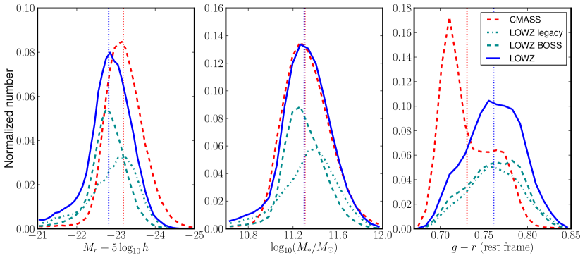
In Figure 1 we show the absolute $r$-band rest frame magnitude, stellar mass, and $g-r$ rest frame color distributions of this sample, K+e-corrected to $z=0$, using values from Maraston et al. (2012). The stellar masses were calculated assuming a Kroupa (2001) initial mass function, including stellar mass loss due to stellar evolution. We also plot distributions for the CMASS sample and split the LOWZ sample into Legacy and new BOSS objects to show the difference between SDSS I/II targets and new BOSS targets. LOWZ galaxies are typically half a magnitude fainter than CMASS galaxies, but CMASS contains more blue galaxies. LOWZ galaxies which were observed as part of SDSS I/II are typically brighter and have $\sim 0.4\,\mbox{dex}$ higher stellar masses, which is to be expected given the brighter magnitude selection imposed as part of that survey. LOWZ galaxies have very similar colors to Legacy galaxies, and are typically redder than CMASS galaxies.

Figure 2: The on-sky distribution (equatorial coordinates) of our sample, with the north and south Galactic caps (NGC and SGC, respectively) labeled for reference. The black regions show the data used in the current study, while the light grey areas are the regions that had to be dropped because of the change in target selection. The background yellow/green color field shows the on-sky density of LOWZ targets in the full BOSS target area, representing the total area that will be covered when the survey is completed in 2014.

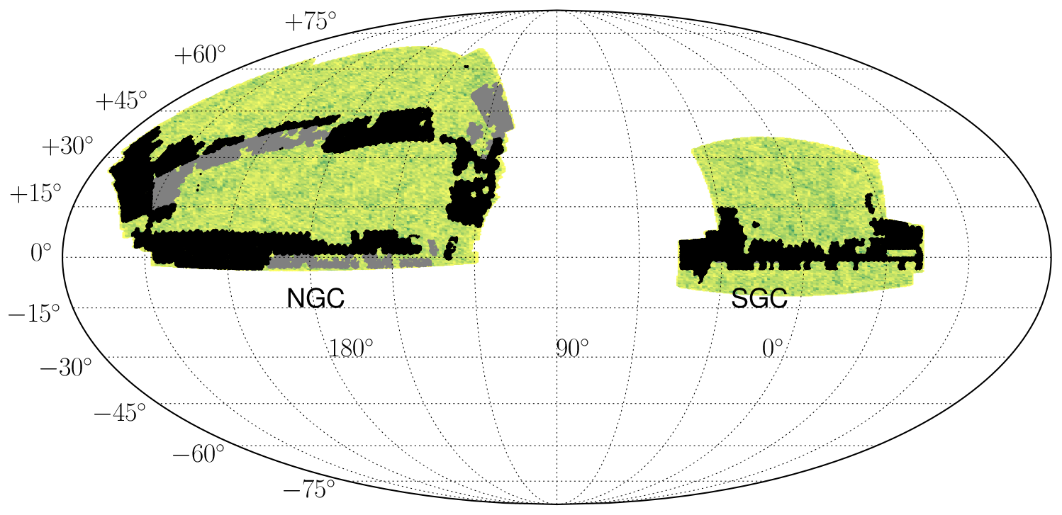
Figure 2 displays the on-sky distribution of the current sample. As noted above, because of changes in target selection we are not able to use roughly the first year’s worth of data. This reduces the total sky coverage compared with the DR9 CMASS sample of Anderson et al. (2012) by $1205$ square degrees ($0.367$ steradians), and removes a large part of the area studied in White et al. (2011). The area with good LOWZ data shown covers $2467$ square degrees ($0.7517$ steradians) on the sky.

We consider data from the North Galactic Cap (NGC) and South Galactic Cap (SGC) separately in our analysis for a number of reasons. We lack a dark matter simulation that resolves the host halos of BOSS galaxies and is large enough to fit the NGC and SGC in a single simulation box. The SGC has a $\sim 8\%$ higher target density than the NGC, and thus a higher galaxy number density, mostly due to differences in photometric calibration and reddening correction between the hemispheres. Schlafly et al. (2010) and Schlafly & Finkbeiner (2011) found a difference in the SDSS colors between the NGC and SGC, resulting in a $0.015\,\mathrm{mag}$ offset in $c_{\parallel}$ (eq. 1 and 3). The “ubercal” SDSS photometry(Padmanabhan et al., 2008) uses overlapping regions of images to cross-calibrate the photometric measurments. As the NGC and SGC are not contiguous they are less well cross-calibrated than they are internally calibrated. This produces some of the measured color difference between the NGC and SGC. Schlafly & Finkbeiner (2011) also identified a slight systematic error in the reddening correction that was applied before targetting. Ross et al. (2011) describe the use of the Schlafly & Finkbeiner (2011) color offsets, determined from stellar spectra, to correct for the north/south asymmetry. They find that the NGC/SGC CMASS and LOWZ number density differences are completely consistent with the level of color offset found by Schlafly & Finkbeiner (2011), but note the inherent uncertainties in the offsets and resulting corrections. They also find that these, and other, systematics more strongly affect the CMASS sample than the LOWZ sample, and are most important for clustering studies on the largest scales. As we will show, the resulting two LOWZ galaxy populations are not significantly different in their clustering properties (see results in Sections 3.2, 4, and 5). We provide values for the NGC and SGC separately, and also provide minimum-variance weighted values for NGC+SGC (hereafter, Full) when appropriate.

Figure 3: The redshift distribution of the BOSS LOWZ sample. The SGC and NGC are plotted separately as dashed and dashed-dotted lines, respectively; showing the higher number density in the SGC. The solid black line gives the total $\bar{{N}}(z)$ distribution for SGC+NGC. Our redshift range of $0.2<z<0.4$ is marked with thin vertical lines. The original survey galaxy density goal of $\bar{{N}(z)}=3\times 10^{-4}h^{3}\mathrm{Mpc}^{-3}$ is shown for reference (thin horizontal line), while the green horizontal lines show the NGC and SGC effective mean density over the $0.2<z<0.4$ range (values given in Table 1)

Table 1: Statistics of the $0.2<z<0.4$ galaxy sample

region	$\mbox{N}_{galaxy}$	$\bar{N}(z)\,(10^{-4}h^{3}\mathrm{Mpc}^{-3}$)
SGC (Legacy)	3946	1.502
SGC (BOSS)	19558	2.681
SGC (Legacy+BOSS)	23504	3.167*
NGC (Legacy)	18332	0.990
NGC (BOSS)	37059	2.005
NGC (Legacy+BOSS)	55391	2.907*
Full (Legacy)	22278	1.053
Full( BOSS)	56617	2.198
Full (Legacy+BOSS)	78895	2.981

The $\bar{{N}}(z)$ values marked with an asterisk are used in the MCMC fitting procedure.

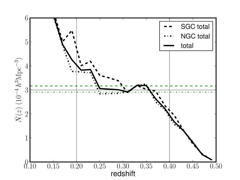
Figure 3 presents the galaxy number density of our samples as a function of redshift. The vertical lines denote the redshift range used in this work ($0.2<z<0.4$). We restrict to this range as it provides a relatively uniform number density across the redshift interval, and to distinguish it from the CMASS sample studied by White et al. (2011), which was restricted to $0.4<z<0.7$. The dramatic increase in the number density below $z\sim 0.2$ is due in part to more than just massive red galaxies falling into the target selection. Additionally, Tojeiro & Percival (2011) and Tojeiro et al. (2012) found that SDSS II LRGs below $z\lesssim 0.2$ had different dynamical growth than LRGs at higher redshifts. A more in-depth study of the uniformity and completeness of the full LOWZ sample is in progress. The difference between the NGC (dash-dotted lines) and SGC (dashed lines) number density is clearly visible in the plot. We present some basic statistics of our sample in Table 1, including separate values for the SGC, NGC, and Full NGC+SGC, and Legacy, BOSS, and Legacy+BOSS redshift samples. One can see the significantly larger number of new BOSS redshifts compared to Legacy in the SGC, as SDSS I/II only observed three stripes in that region covering about $700$ square degrees, compared with $3100$ square degrees of imaging available to BOSS (Aihara et al., 2011). The BOSS redshift densities in the two hemispheres should not be directly compared, because of the different number of Legacy redshifts in the NGC vs. SGC.

3 Real Space Clustering

3.1 Measurements

The correlation function $\xi(r)$ (Peebles, 1980) measures the excess probability of finding a galaxy in a volume element, $dV$, at separation $r$ from a randomly selected galaxy,

$$dP(r)=N_{G}(1+\xi(r))dV,$$ (7)

where $N_{G}$ is the mean galaxy number density. We use the estimator of Landy & Szalay (1993),

$$\xi(r)=\frac{DD-2DR+RR}{RR}.$$ (8)

Compared to the “natural” estimator $DD/RR-1$, the Landy and Szalay estimator reduces geometrical edge effects and minimizes variance.

Figure 4: Left panel: contours of the correlation function $\xi(r_{\perp},r_{\parallel})$ (smoothed with a Gaussian kernel of radius $0.5\,h^{-1}\mathrm{Mpc}$ for clarity) of the components parallel ($r_{\parallel}$) and perpendicular ($r_{\perp}$) to the line of sight, for BOSS LOWZ galaxies with redshifts in the range $0.2<z<0.4$. In both plots the blue lines show results for NGC data and green lines show results for SGC data. Solid contours are shown at $\xi=(1,2,4,8)$, dashed contours at $\xi=(0.5)$, and a thicker solid line is shown for $\xi=1$. Thin black dotted circles are plotted for $\xi(r)=(2,1,0.5)$ for reference. Right panel: the same, but for our mock galaxy catalog (Section 3.3). Note that similar features (e.g. finger-of-god) are present in the mocks. In both panels, the discontinuity at $r_{\parallel}=0$ is due to small number fluctuations in the smallest bins.

We use this estimator to calculate a two-point galaxy correlation function of pair separations parallel ($r_{\parallel}$) and perpendicular ($r_{\perp}$) to the line of sight, $\xi(r_{\parallel},r_{\perp})$. We then compute the projected correlation function, $\omega_{p}(r_{\perp})$, which reduces the effect of redshift-space distortions, by integrating,

$$\omega_{p}(r_{\perp})=2\int_{0}^{r_{\parallel,\mathrm{max}}}\xi(r_{\parallel},r_{\perp})dr_{\parallel},$$ (9)

where we take $r_{\parallel,\mathrm{max}}=75h^{-1}\mathrm{Mpc}$ as the upper limit of the integral. The integral is stable around this value, while not contributing noise from large $r_{\parallel}$ bins. The relationship between the projected correlation function, $\omega_{p}(r_{\perp})$ , and the real-space correlation function is (e.g. Davis & Peebles, 1983)

$$\omega_{p}(r_{\perp})=2\int_{0}^{y_{\mathrm{max}}}\xi[(r_{\perp}^{2}+y^{2})^{1/2}]dy$$ (10)

which is used in our full-box mock simulations to more quickly compute $w_{p}(r_{\perp})$ (see Section 3.2). We again integrate to $y_{\mathrm{max}}=75h^{-1}\mathrm{Mpc}$ as a balance between including most of the information from the correlation function, and limiting noise from large radius bins. We tested and confirmed that this integral produces almost identical results to the integral over the correlation function in Eq. 9, as long as $\xi(r)$ is measured in small enough bins to allow for smooth interpolation.

Not all galaxy targets in each region on the sky were assigned spectroscopic fibers. Specifically, the completeness of the survey varies between the different regions defined by sectors which consist of disjoint regions defined by the overlap of spectroscopic tiles. In addition, as mentioned above, some of our targets come “pre-observed”, i.e., with redshifts from SDSS I/II. We thus separate galaxies into two groups and calculate their completeness, fgot, on a per-sector basis as

$$\mathrm{fgot}_{\mathrm{BOSS}} = N_{\mathrm{BOSS}}/(N_{\mathrm{targets}}-N_{\mathrm{Legacy}})$$ (11)

$$\mathrm{fgot}_{\mathrm{Legacy}} = 1$$

where $N_{\mathrm{BOSS}}$ is the number of new, not confirmed as star, BOSS redshifts, $N_{\mathrm{targets}}$ is the number of LOWZ targets and $N_{\mathrm{Legacy}}$ is the number of previously acquired Legacy redshifts that were targeted per the algorithm described above. For Legacy redshifts the completeness is defined to be 1, as they can be considered a separate, fixed, sample whose redshifts are pre-determined. Known Legacy redshifts were excluded during targeting, so they do not affect whether any BOSS targets were allocated a fiber. If $N_{\mathrm{targets}}-N_{\mathrm{Legacy}}=0$, the sector is assigned a completeness of $1$, as all of the targets have Legacy redshifts, and no new BOSS redshifts were required.

When computing the correlation function, we weight galaxies by $\mathrm{fgot}^{-1}$ (see Eq. 11), restricted to only those galaxies which lie in sectors with $\mathrm{fgot\mbox{}}>0.5$. For calculating the correlation function, we generate random points uniformly in all regions with $\mathrm{fgot}>0.5$, and assign all randoms a weight of $1$. We generate $100$ times the number of data points for our random catalog as we have observations, ensuring the variance of the results is not affected by the random catalog. We assign redshifts to the randoms by smoothing the NGC and SGC redshift distributions with a 7th order Chebyshev polynomial and drawing from each of the resulting distributions separately for the NGC and SGC random catalogs, respectively.

To correct for fiber-collisions, we use the nearest-neighbor redshift method (Zehavi et al., 2002, 2005a; Berlind et al., 2006). To each galaxy within a “collision group” that does not have a good redshift, we assign the redshift of the nearest galaxy within $62\arcsec$. Although this method is known to over-correct below the fiber-collision radius ($62\arcsec$ for BOSS, corresponding to $0.235h^{-1}\mathrm{Mpc}$ at the highest redshift in our sample), it is a nearly exact correction at radii larger than twice the fiber-collision radius. Guo, Zehavi & Zheng (2011) demonstrated a more exact method for corrections below the fiber-collision radius, but their method reduces the number of points included in the correlation function calculation, and thus increases the variance of the measurement. As the smallest radius bin we consider is well above the fiber-collision radius, and the results of Guo, Zehavi & Zheng (2011) show close correspondence between their new method and the nearest neighbor method for large radii, we will adopt the simpler method in this work.

Figure 5: Left: NGC and SGC, data and mocks. Right: NGC+SGC Full sample. In each plot, the upper panel shows the projected correlation function for BOSS LOWZ galaxies with redshifts in the range $0.2<z<0.4$. Dashed lines show the mean (not the single best-fitting model) mock correlation functions from our MCMC fitting procedure. Errors are computed from the square-root of the diagonal of our covariance matrix, generated using the mean HOD parameters. The thin line shows a simple best-fit power law, $\xi_{PL}=\left(\frac{r}{r_{0}}\right){}^{-\gamma}$, transformed to $w_{p,PL}(r_{\perp})$ using eq. 10, to guide the eye. Also plotted on the right is the mean CMASS correlation function from White et al. (2011) for comparison. The lower panels show the same curves as above, but with each curve divided by the power law fit to emphasize the differences between the various correlation functions, and to show that a pure power law fit is not appropriate for this data. The NGC and SGC correlation functions match within the errors. The correlation functions clearly display the inflection at $1-2h^{-1}\mathrm{Mpc}$ that marks the transition between the one-halo and two-halo regimes (Zehavi et al., 2004).

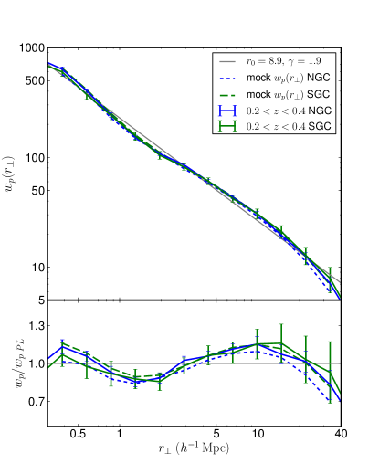
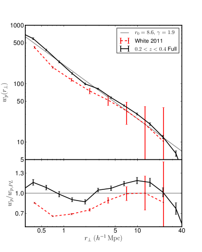
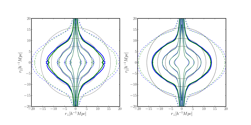
We show the correlation function contours in $(r_{\parallel},r_{\perp})$ in Figure 4, alongside the mock catalog 2D correlation function for comparison. The mocks show similar redshift space distortions to the data, with Fingers-of-God and large scale squashing due to the Kaiser effect (Kaiser, 1987) clearly evident. Our procedure for generating the redshift space mock catalogs is described in Section 3.3. Following Eq. 9, we integrate this 2D correlation function to get the projected correlation function, $w_{p}(r_{\perp})$ shown inFigure 5. The errors are estimated from our mock catalogs (see Section 3.2), shifted onto the sky and masked with the coverage map. As noted in Section 2, we present the NGC and SGC separately in the left-hand figure, and the minimum-variance weighted Full NGC+SGC in the right-hand figure. It is clear from the figure that over the scales considered in this paper, the clustering of the NGC and SGC are the same within the errors, differing by less than $1\sigma$. The CMASS errors from White et al. (2011)on large scales are significantly larger than ours, because that analysis was performed on a much smaller data set ($580\mbox{deg}^{2}$, or roughly $30\%$ the solid angle). The large scale errors are determined primarily by the volume of the survey, so our increased volume improves on those errors. In addition, the geometry of the White et al. (2011) sample naturally split into three disjoint regions, A, B, and C, reducing the number of large-scale pairs.

Table 2: The projected correlation function, $w_{p}(r_{\perp})$, in 12 equally spaced bins in $\log_{1.5}(r_{\perp})$.

$r_{\perp}$	0.385	0.577	0.865	1.299	1.945	2.921	4.381	6.572	9.858	14.78	22.18	33.27
Full $w_{p}(r_{\perp})$	619.29	390.51	242.17	153.87	106.83	84.18	60.42	43.19	30.70	19.83	12.66	7.22
Full $\sigma$	27.20	18.80	9.51	5.60	4.60	3.17	2.30	1.76	1.69	1.36	0.85	0.87
NGC $w_{p}(r_{\perp})$	632.95	404.09	242.84	152.32	107.88	85.42	60.33	43.41	30.70	19.52	12.63	7.07
SGC $w_{p}(r_{\perp})$	598.26	372.80	240.20	156.64	104.49	81.68	60.67	42.25	30.72	21.11	12.83	7.90
NGC $\sigma$	31.49	15.53	12.40	6.735	4.888	2.746	2.292	1.527	1.584	1.376	1.042	0.9794
SGC $\sigma$	52.58	36.36	25.99	13.78	8.555	5.376	4.354	3.322	3.138	2.755	2.309	2.070
0.385	1	0.5380	0.5110	0.4830	0.2790	0.2380	0.3510	0.3610	0.4470	0.3110	0.2710	0.2040
0.577	…	1	0.5150	0.4910	0.3680	0.4150	0.4730	0.3860	0.2860	0.2860	0.2470	0.2990
0.865	…	…	1	0.7090	0.6460	0.4640	0.3520	0.3910	0.3420	0.3250	0.1880	0.1430
1.299	…	…	…	1	0.6150	0.5100	0.4710	0.5010	0.5690	0.4310	0.2470	0.0740
1.945	…	…	…	…	1	0.6180	0.6120	0.6850	0.5140	0.4520	0.4120	0.2920
2.921	…	…	…	…	…	1	0.6570	0.5130	0.4550	0.3870	0.2620	0.1710
4.381	…	…	…	…	…	…	1	0.7850	0.7230	0.6470	0.5540	0.3980
6.572	…	…	…	…	…	…	…	1	0.7550	0.6200	0.4710	0.2550
9.858	…	…	…	…	…	…	…	…	1	0.8300	0.5600	0.2640
14.78	…	…	…	…	…	…	…	…	…	1	0.7980	0.5350
22.18	…	…	…	…	…	…	…	…	…	…	1	0.8750
33.27	…	…	…	…	…	…	…	…	…	…	…	1

Note: All bin values are in $h^{-1}\mathrm{Mpc}$, at the volume-weighted bin center:$((r_{\mathrm{top}}^{3}+r_{\mathrm{bottom}}^{3})/2)^{1/3}$. The lower part of the table lists the upper triangle of the covariance matrix as $C_{ij}/(\sigma_{i}\sigma_{j})$.

We provide the correlation function and error estimates in Table 2 for the NGC, SGC and Full NGC+SGC samples. The values for the Full sample are computed from a minimum-variance weighted combination of the NGC and SGC. The bins shown are those used during the fitting procedure described below. In the same table, we show the covariance matrix for the Full NGC+SGC data set. The galaxy and random catalogs used in this analysis are available on the SDSS III website.

3.2 Halo Occupation Distribution

We estimate the errors in the sample and determine the dark matter halo statistics using 20 dark matter simulations. These are the same simulations used in the CMASS analysis of White et al. (2011), with $1500^{3}$ particles of mass $7.6\times 10^{10}h^{-1}M_{\odot}$ in a periodic cube $1500h^{-1}\mathrm{Mpc}$ on a side. All 20 simulations have the same cosmological parameters: $\Omega_{M}=0.274$, $\Omega_{\Lambda}=0.726$, $w=-1.00$, $\Omega_{b}=0.0457$, $h=0.70$, $n=0.95$, $\sigma_{8}=0.8$, the same as the parameters given in the introduction for our redshift to distance conversion. We identify dark matter halos using a friends-of-friends (FoF) algorithm (Davis et al., 1985), with a linking length of 0.168. This results in a minimum resolved halo mass for our redshift slice ($z=0.30$) of $10^{11.88}h^{-1}M_{\odot}$. For more details on these simulations, see the appendix of White et al. (2011). Note that we are not fitting cosmological parameters, and our CMASS comparison is straightforward because the assumed cosmologies are exactly the same.

We do not have a single cosmological simulation with a sufficiently large volume and a high enough number density to embed the NGC and SGC in the same box, but our simulations are large enough if the NGC and SGC are considered separately. We can safely ignore correlations between the NGC and SGC in this analysis, as the shortest distance between an NGC and an SGC galaxy is $53{}^{\circ}$–corresponding to $>600\,h^{-1}\mathrm{Mpc}$ at the sample’s minimum redshift–while this paper only considers separations below $40\,h^{-1}\mathrm{Mpc}$. Our technique of fitting each separate region into our simulation cubes to generate mock galaxy catalogs for error estimation is discussed in Section 3.3.

For an accurate interpretation of galaxy clustering, we use the halo occupation distribution (HOD) formulation (Peacock & Smith, 2000; Seljak, 2000; Benson et al., 2000; White, Hernquist & Springel, 2001; Scoccimarro et al., 2001; Berlind & Weinberg, 2002). The HOD gives the conditional probability that a halo with virialized mass $M_{\mathrm{halo}}$ contains $N$ galaxies of a particular class. In this paper, we distinguish central and satellite galaxies, and we require that halos with a satellite must have a central galaxy.

We determine the number of satellite and central galaxies in each halo following a halo prescription based on that of Zheng et al. (2005) with a central galaxy probability of

$$N_{\mathrm{cen}}(M_{\mathrm{halo}})=\frac{1}{2}\mathrm{erfc}\left[\frac{\ln(M_{cut}/M_{\mathrm{halo}})}{\sqrt{2}\sigma}\right],$$ (12)

and an expected number of satellites equal to

$$N_{\mathrm{sat}}(M_{\mathrm{halo}})=\left(\frac{M_{\mathrm{halo}}-\kappa M_{cut}}{M_{1}}\right){}^{\alpha},$$ (13)

where $M_{cut}$, $M_{1}$, $\sigma$, $\kappa$, and $\alpha$ are the free-parameters to be fit in our model, described in detail in Appendix A. Briefly, $M_{cut}$ is a minimum mass for halos to host our galaxies, $M_{1}$ is a typical mass for halos to host one satellite, $\sigma$ is the scatter between $M_{*}$ and $M_{\mathrm{halo}}$, $\kappa$ allows the threshold mass for satelites and centrals to differ, and $\alpha$ is the mass dependence of the efficiency of galaxy formation. This halo prescription was created to reproduce the observed luminosity-dependent clustering and number densities from the SDSS main galaxy (Strauss et al., 2002) and LRG samples (Eisenstein et al., 2001). We assume that for a halo to contain satellites it must first contain a central, so we only assign satellites to halos with a central galaxy. Thus, the total expected number of galaxies in a halo of mass $M_{\mbox{halo}}$ is

$$\langle N_{\mathrm{gal}}(M_{\mathrm{halo}})\rangle = \langle N_{\mathrm{cen}}(M_{\mathrm{halo}})\rangle(1+\langle N_{\mathrm{sat}}(M_{\mathrm{halo}})\rangle).$$ (14)

We assign central galaxies to halos when a uniform random deviate is less than the value of Eq. 12 for that halo. We then compute the number of satellites in each halo hosting a central by selecting a value from a Poisson distribution with $\lambda=N_{\mathrm{sat}}$ as given by Eq. 13.

We assign central galaxies to the halo center position and place satellites at the position of a randomly-selected dark matter particle within the halo. This eliminates the common assumption of spherical NFW profiles (Navarro, Frenk & White, 1996) and preserves the non-spherical halo shapes. In a study of how halo occupation assumptions affect galaxy clustering statistics, Zu et al. (2008) and van Daalen, Angulo & White (2012) both found that assuming spherical halos could decrease the measured correlation function by up to $\sim 10-20\%$ on scales below $r\lesssim 1h^{-1}\mathrm{Mpc}$, compared to the clustering measured with the true halo shapes. They also reported a reduction in the correlation function on scales of a few $h^{-1}\mathrm{Mpc}$ if the halos are not correctly aligned within the overall large scale structure. By placing galaxies at the location of dark matter particles within each halo, we preserve both the halo shape and the overall halo alignment. An even better choice would be to place the galaxies at the locations of subhalos, but our simulations do not have the resolution to track individual subhalos. In either case, this method more correctly reproduces the 1-halo/2-halo transition region of the correlation function (Cooray & Sheth, 2002; Zehavi et al., 2004) than distributing galaxies via spherical NFW profiles.

See Appendix A for details on the physical motivations of these HOD parameters and examples of how they each affect both the shape of the HOD and the resulting correlation function.

3.3 Error estimates

We perform our fitting procedure below on the projected measurements (e.g., Eq. 9 and Figure 5), without incorporating information about the galaxy peculiar velocity field. To estimate measurement errors, we must shift our mock catalogs from real into redshift space, place them on the sky, and mask them with the geometry. In addition, we effectively double the number of available mock galaxy catalogs by flipping each simulation around one axis when generating the mock galaxy catalog below, to double our effective number of simulation boxes from 20 to 40. The flip is chosen to minimize (NGC) or eliminate (SGC) overlap between the flipped and non-flipped versions of the box. The overlap in the NGC between the flipped and non-flipped boxes is less than 10%, so there should be minimal signal in the covariance matrix due to this procedure. Since the geometry of our simulations is a cube, while the survey geometry is a much more complicated region defined by sectors on the sky (described at the end of Section 2, and represented graphically in Figure 2) and a radial selection function (i.e., Figure 3), we remap the periodic simulation cube into a rectangular parallelepiped via the method and code of Carlson & White (2010), and then restrict it to the on-sky mask (see Figure 2).

The remapping procedure applies a shear transformation to the periodic simulation cube. Because the simulation box is periodic, we embed a new sheared box into the infinite tiling of periodic boxes and take the new catalog be the points at their new, sheared, positions. This transformation preserves the simulation volume and number density and contains each point once and only once (see Figure 2 in Carlson & White (2010) for a 2d graphical representation of this procedure). This remapping procedure requires that the box size of the simulations be large enough so that it preserves large scale structure–an excessively thin sheared box will remap too many distant points to be in close neighborhoods. Note that we also must rotate the galaxy velocities (described below) by a rotation matrix defined by the normalized basis vectors defining the new sheared box. This places the galaxy velocity vectors, originally in the coordinate system of the simulation cube, in the coordinate system of the remapped box.

We then embed the survey geometry into the remapped simulation box on the sky. We shift the origin of the coordinates of the simulation box so that its minimum $(x,y,z)$ coordinate corresponds to the minimum $(x,y,z)$ coordinate for the data (in the NGC, and SGC separately), effectively placing the mock galaxy box on the sky in the same location as the galaxy data, but covering a larger area.

To convert our mock catalogs into redshift space, we must assign a peculiar velocity to each galaxy. Central galaxies are assigned the bulk velocity of their host halos, which should produce a flattening of the correlation function along the line of sight due to large scale motion (Kaiser, 1987). For satellites, we assign the peculiar velocity of each galaxy’s associated dark matter particle, as this includes both the bulk halo motion and the infall velocity. This should result in Fingers-of-God. As our simulation velocities are “distance offsets” relative to the position coordinates, we can convert the real space coordinates, $r$, into redshift space coordinates, $s$, via

$$s=r+\hat{r}\cdot\overrightarrow{v},$$ (15)

where $\overrightarrow{v}$ is the galaxy velocity as given above and $\hat{{r}}$ is the line-of-sight unit vector from the observer’s coordinates $(0,0,0)$ to the galaxy. We then restrict the on-sky coordinates of the galaxies to the area described in Section 2.

To measure the correlation function on these redshift space mocks, we use exactly the same binning as was used for the data, measuring either $\xi(s)$ directly, or $w_{p}(r_{\perp})$ by integrating Eq. 9. The error bars shown in Figures 5 and 8 and the covariance matrix used in the MCMC procedure and listed in Table 2 are computed from the standard deviation of the 20 mock galaxy correlation functions.

3.4 MCMC fitting

To determine the best-fit HOD parameters, we use a Markov Chain Monte Carlo (MCMC) method to fit $w_{p}(r_{\perp})$ and the overall galaxy number density, as measured from the BOSS data. In particular, we use the Metropolis-Hastings MCMC formalism (Metropolis et al., 1953; Hastings, 1970), with errors on $w_{p}(r_{\perp})$ from the mock catalogs and assuming a fixed $15\%$ error on the galaxy density (see below for justification). This method starts with an initial seed set of values for the HOD parameters and then,

1. Computes a step in a direction determined from the covariance of the parameters (as discussed in Appendix A).

2. Populates the dark matter simulation with galaxies according to that HOD.

3. Computes $\xi(r)$ on the resulting mock galaxy catalog.

4. Integrates $\xi(r)$ to obtain $w_{p}(r_{\perp})$ via Eq. 10.

5. Computes the $\chi^{2}$ between the model and the data.

We accept the new HOD parameters with probability:

$$\mbox{P}=\min(1,e^{-(\chi_{new}^{2}-\chi_{old}^{2})/2}).$$ (16)

We then iterate this procedure for at least $25,000$ steps, thus filling out the most likely region of parameter space, which allows us to easily determine the most likely value and scatter of any statistic derived from the HOD parameters. For the first run of the MCMC procedure, we bootstrap with fixed 20% errors on all correlation function points, and then use the error estimated from this fit in the following run. In each subsequent MCMC run, we use the errors on $w_{p}(r_{\perp})$ estimated from the previous run (see Section 3.3 for how the error estimates are generated), and iterate this process until convergence, defined as the mean correlation function of two runs being the same within the $1\sigma$ errors. The fitted parameters converge after 3-4 MCMC runs, and the best-fit and mean values, and estimated errors given in this paper, are taken from the final run.

Although the galaxy number density (Figure 3) varies by $\gtrsim 30\%$ across our redshift range, the mock-to-mock variance in galaxy number density is $\sim 2\%$. The survey is not volume limited, while the mocks are, by construction. In our MCMC fits, we chose a $15\%$ error on $\bar{{N}}(z)$ to allow for variation across the redshift range, while still restricting the MCMC code to values close to the mean of the survey. Through testing, we found that a tighter restriction, e.g. 5%, prevents the chains from converging on a solution. A more complete mock catalog generation process would assign luminosities and colors to the galaxies and observe them on the sky in the same manner that the data was observed, resulting in a mock catalog with a redshift distribution closer to that of the data (e.g. the method of Skibba & Sheth, 2009).

Because of variance between simulations, we perform our MCMC fitting on the “mean” simulation, defined as follows. We compute the correlation function, $\langle\xi(r)\rangle$, of halos with $M_{halo}>10^{13}h^{-1}M_{\odot}$, and select the simulation with the smallest sum-of-squares difference from the mean of the 20 correlation functions. This ensures that our correlation function fitting procedure is not biased high or low due to a particular simulation box having particularly high or low inherent halo clustering. Restricting to high mass halos is a rough proxy for the halos occupied by our galaxies, without any of the randomness involved in assigning centrals and satellites to halos. An alternative to choosing the “mean” simulation would be to perform the fitting procedure on all 20 simulations at once, but this is computationally prohibitive.

We fit the correlation function in the 12 radial bins given in Table 2, plus the average galaxy number densities given in Table 1. When combined with our 5 parameter model, there are 7 degrees of freedom for the $\chi^{2}$-test portion of the MCMC. Our mean HOD model has a $\chi^{2}$ of $7.35$ for the NGC and $5.73$ for the SGC.

Table 3: The mean and standard deviation of the HOD parameters (see Eq. 12 and 13).

parameter	mean Full	mean NGC	best-fit NGC	mean SGC	best-fit SGC
$\log_{10}M_{cut}/M_{\odot}$	$13.25\pm 0.26$	$13.17\pm 0.14$	$13.16$	$13.09\pm 0.09$	$13.11$
$\log_{10}M_{1}M_{\odot}$	$14.18\pm 0.39$	$14.06\pm 0.07$	$14.11$	$14.05\pm 0.09$	$14.07$
$\sigma$	$0.70\pm 0.40$	$0.65\pm 0.27$	$0.741$	$0.53\pm 0.28$	$0.692$
$\kappa$	$1.04\pm 0.71$	$1.46\pm 0.44$	$0.921$	$1.74\pm 0.74$	$1.26$
$\alpha$	$0.94\pm 0.49$	$1.18\pm 0.18$	$1.38$	$1.31\pm 0.19$	$1.31$

Figure 6: Halo Occupation Distributions (HODs) for LOWZ (NGC+SGC) and CMASS samples compared with HODs for two samples of LRGs with photometric redshifts from SDSS I/II (“DR6: 2” with a mean redshift of $0.326$ and “DR6: 3” with a mean redshift of $0.376$). The dashed lines shows the expected number of centrals, dashed-dotted lines show expected number of satellites, and solid lines show the total number of galaxies as a function of halo mass. The shaded region shows the $\pm 1\sigma$ variation determined by our MCMC fitting procedure.

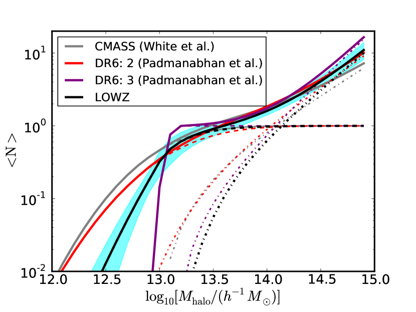
Our MCMC procedure produces the mean (calculated from all MCMC steps) and best-fit (lowest single $\chi^{2}$ during the MCMC procedure) parameters shown in Table 3. The parameter $\kappa$ is poorly constrained, and although $\sigma$ is also not strongly constrained, it is below the value for the CMASS sample ($0.98\pm 0.24$). We estimate our errors from the mean HOD parameters, not the best-fit, as the single best-fit value is partly determined by random variations in the mock correlation functions. Figure 6 presents the mean number of galaxies per halo. We also show, for reference, the HOD determined for the CMASS sample of White et al. (2011), and two HODs selected from Padmanabhan et al. (2009) that represent galaxies with photometric redshifts in a similar redshift and mass range to those in our current sample. The LOWZ sample clearly lies between the Padmanabhan et al. (2009) samples 2 and 3, with a steeper cutoff for central galaxies than sample 2. The behavior of the HOD at low halo masses is driven primarily by the amplitude of the correlation function; the relatively large measured clustering amplitude (compared with, e.g. CMASS) agrees well with our steep cutoff in the average number of galaxies in low mass halos. Within the HOD framework, galaxies with a high bias must occupy high mass halos, resulting in a sharper turnoff in the central galaxy fraction. For a more detailed comparison with CMASS, see Section 5.

Figure 7: Probability distribution (normalized to have an integral of 1) of satellite fractions for NGC and SGC.

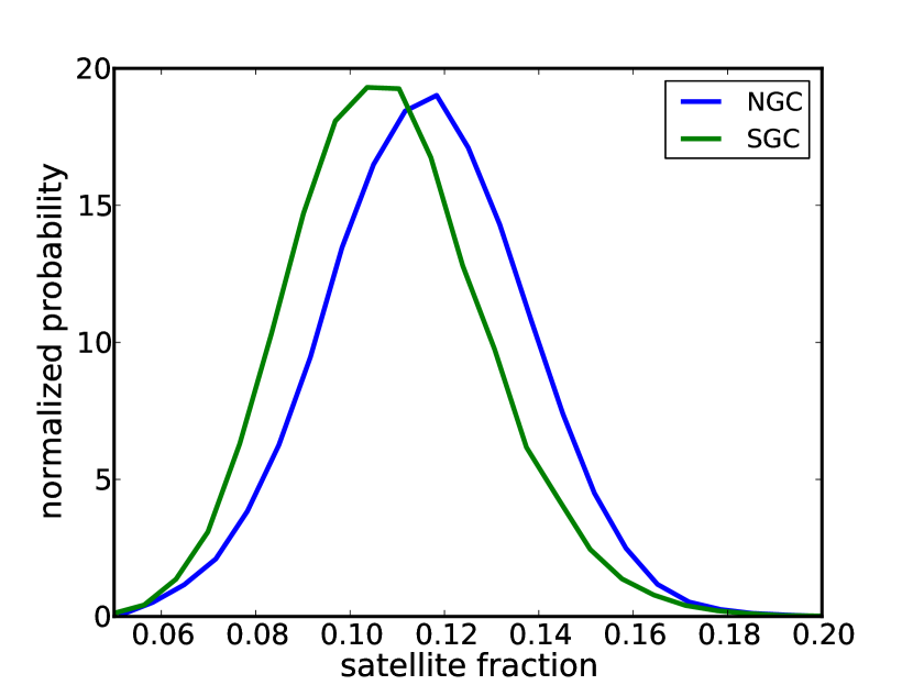
Our results suggest that $12\pm 2\%$ of NGC and $11\pm 2\%$ of SGC galaxies are satellite galaxies in their halos instead of centrals. This is comparable with the $\sim 10\%$ satellite fraction measured by White et al. (2011) for the higher redshift CMASS sample. We show the probability distribution function (PDF) of satellite fraction in Figure 7. There is considerable overlap between the NGC and SGC satellite fraction PDFs, and we find these results to be statistically indistinguishable.

4 Redshift Space

Figure 8: Left: NGC and SGC, data and mocks. Right: NGC+SGC Full sample. Upper panels: the redshift space correlation function for BOSS LOWZ galaxies with redshifts in the range $0.2<z<0.4$. The thin line shows the same best-fit power law from Figure 5 with $s_{0}=8.9$, $\gamma=1.9$. The dashed lines show the mean of the 20 mock catalogs generated from our simulations, using the mean HOD parameters given in Table 3. Lower panels: the same curves as above, but divided by the mean of the NGC and SGC to emphasize the differences between the various correlation functions. The thin solid line at $\xi(s)/mean(NGC,SGC)=1$ is not the powerlaw from the upper panel, but is just shown for reference.

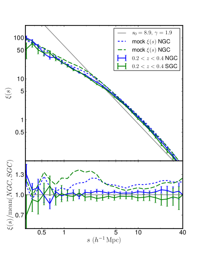
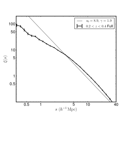
As a test of our HOD fits, we compute the redshift space correlation function for the data, and for our mean HOD parameters. As our HOD fitting procedure does not incorporate any information about the velocity distribution of the galaxy sample, this approach provides a convenient check of our results.

Figure 8 shows the redshift-space correlation function, $\xi(s)$. We also plot the same power law from Figure 5 and the mean redshift space mock catalogs for comparison. The effects of redshift space distortions are clear here, with a decrease in the correlation function amplitude at small scales, and an increase at larger scales.

The mocks in this case were not fit to the data, but rather were computed using the HOD parameters that were fit to the $w_{p}(r_{\perp})$ measurements. The differences between the data $\xi(s)$ and mock $\xi(s)$ could be due to our requirement that every halo with satellites must have a central: the lower luminosity galaxies in our sample may be satellites in halos that do not have a LOWZ galaxy as their central. The difference may also reflect deviations from our assumption that the galaxies strictly follow the motion of individual dark matter particles, as opposed to the subhalos that they truly do occupy. Further work could expand on this issue by, for example, making different assumptions about satellites and centrals, selecting subsets of LOWZ galaxies with different colors and luminosities, or having the galaxies follow proper subhalos instead of individual dark matter particles (see, e.g., Seljak, 2001; White, 2001; Scoccimarro, 2004; Skibba et al., 2006; Tinker, Weinberg & Zheng, 2006).

5 Comparison with previous work

Figure 9: The probability that a galaxy lies in a halo of a given mass, comparing CMASS and the NGC and SGC LOWZ sample. Because the HOD for LOWZ galaxies is more sharply truncated than the CMASS HOD, LOWZ galaxies do not probe halos with masses as small as the those of the CMASS sample.

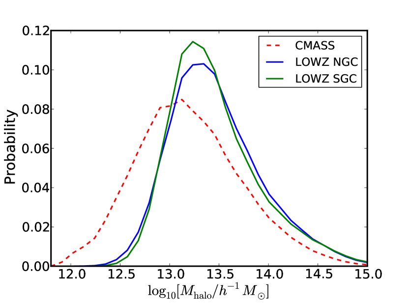
Figure 9 shows a different view on the halo occupation of these galaxies: the probability that a galaxy lies in a halo of mass $M$. We compute the mean halo mass to be $5.2\times 10^{13}h^{-1}M_{\odot}$ for the LOWZ sample. This Figure clearly shows the sharper halo occupation cutoff at low halo masses, compared with the CMASS sample, which had a mean halo mass roughly half as large. This difference is likely due to the fact that our galaxies are redder than CMASS (Figure 1), and thus would tend to occupy higher mass halos (see, e.g., Skibba et al., 2009). In addition, a galaxy population undergoing dynamical passive evolution would occupy higher mass halos with cosmic time, as their original host halos merge to form more massive halos. This is consistent with the fact that there is little difference between the LOWZ and CMASS stellar masses (Figure 1): these galaxies have undergone considerable halo growth, but little to no stellar mass growth since $z\sim 0.5$ (see also White et al., 2007; Brown et al., 2008; Wake et al., 2008).

Figure 10: The scale dependence of the galaxy bias, $b=\sqrt{\xi_{gal}/\xi_{DM}}$, for the LOWZ sample. The large-scale bias asymptotes to $\sim 2.0$. The strong increase toward scales below $1h^{-1}\mathrm{Mpc}$ appears because of the strong clustering of galaxies within halos, while the bump at the few $h^{-1}\mathrm{Mpc}$ scale is due to one-halo/two-halo transition. The dashed red line shows the galaxy bias of the CMASS sample of White et al. (2011), while the dot-dashed blue line shows the LOWZ galaxy bias relative to the linear theory $\xi_{\mathrm{DM}}$ computed with CAMB.

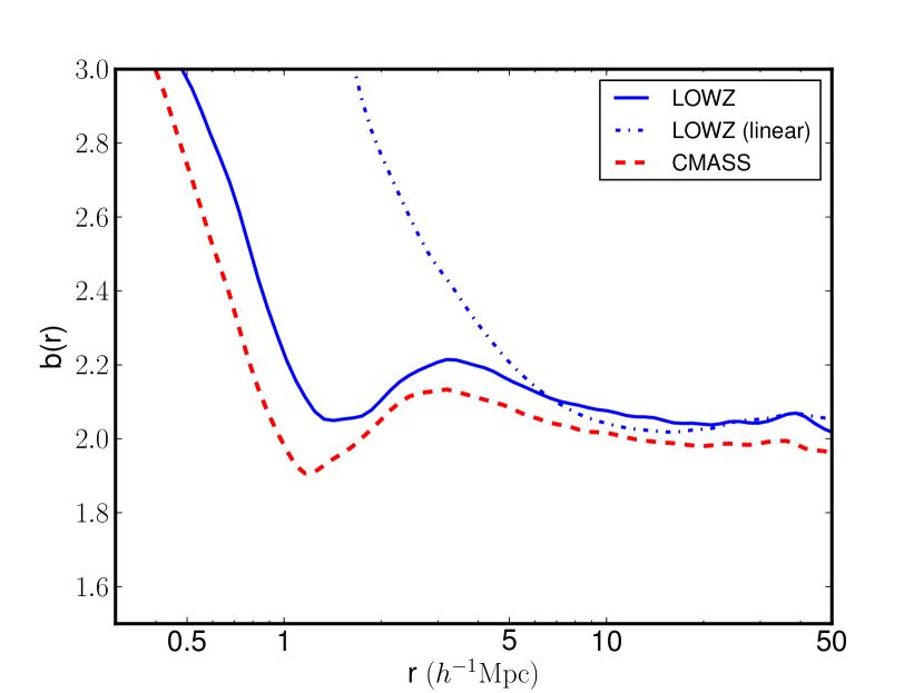
Based on our halo fitting, we can estimate the bias of this galaxy population with respect to the underlying dark matter distribution,

$$b(r)=\sqrt{\frac{\xi_{gal}(r)}{\xi_{DM}(r)}},$$

where $\xi_{gal}(r)$ is the correlation function of the mean galaxy mock (see Table 3), and $\xi_{DM}(r)$ is the correlation function of dark matter in our simulations. We find a large scale galaxy bias of $\sim 2.0$ and show the scale dependence of the bias in Figure 10. The dot-dashed blue line shows the bias relative to the linear theory correlation function from CAMB (Lewis, Challinor & Lasenby, 2000; Howlett et al., 2012), using the same cosmological parameters as our simulations. The linear bias differs from the non-linear bias on small scales but is similar on large scales, as expected. We find a similar bias to that reported for the CMASS sample of White et al. (2011) (dashed red line).

The measured bias of the full CMASS and LOWZ samples is inconsistent with pure dynamical passive evolution of CMASS into LOWZ. In a dynamical passive evolution model in our cosmology, the bias of a galaxy population evolves like

$$b(z_{0}\rightarrow z)=(b_{z_{0}}-1)\frac{D(z_{0})}{D(z)}+1$$ (17)

(Fry, 1996). Thus, a bias of $2$ at $z=0.55$ should evolve to $1.88$ at $z=0.3$. Equivalently, the $z=0.55$ progenitors of a galaxy population with $b(z=0.3)=2$ should have $b(z=0.55)=2.13$. Tojeiro et al. (2012) suggest that the progenitors of SDSS II LRGs are preferentially located in the redder parts of the color/luminosity selection space. Together, this suggests that the LOWZ sample could have passively evolved from a redder, slightly more biased subset of the CMASS sample. Further work fitting HODs at high redshift and evolving them to low redshift (e.g. Zheng, Coil & Zehavi, 2007; White et al., 2007; Wake et al., 2008), as well as selecting subsets of the CMASS sample that may be more representative of the LOWZ progenitors could clarify this issue.

Zehavi et al. (2005b) and Zheng, Coil & Zehavi (2007) studied $200,000$ galaxies from the SDSS I/II main sample in the redshift range $0.01<z<0.23$, with the latter using the same correlation function measurements but a more complicated form for the HOD. Their samples were all less luminous than the LOWZ sample, with the most luminous sample having $-23<M_{r}<-22$ and $0.1<z<0.23$. They found a large-scale bias factor of $1.91$ for the most luminous sample, with the other samples having smaller bias. They also measured the mean halo mass to be higher for fainter red galaxies $\sim 2\times 10^{14}h^{-1}M_{\odot}$ than for those of intermediate luminosities $\sim 1\times 10^{14}h^{-1}M_{\odot}$. Both of these mean halo masses are significantly higher than the mean halo mass we find for LOWZ galaxies. Zheng, Coil & Zehavi (2007) also added clustering measurements from $30,000$ DEEP2 galaxies in the redshift range $0.7<z<1.45$. The bias of this sample ranged from $1.22$ to $1.45$ for the lower ($M_{B}<-19.0$) and higher luminosity ($M_{B}<-20.5$) samples, respectively. They found satellite fractions for the luminous SDSS and DEEP2 samples (both $\sim 10\%$) similar to our LOWZ results. The results of Zheng, Coil & Zehavi (2007) were updated in Zehavi et al. (2011), incorporating the completed SDSS I/II main sample galaxy catalog. Their two most luminous samples, with $M_{r}^{\mathrm{max}}>-22.0$ ($z<0.245$, $\bar{N}=0.5\times 10^{-4}h^{3}\mathrm{Mpc}^{-3}$) and $M_{r}^{\mathrm{max}}>-21.5$ ($z<0.199$, $\bar{N}=2.8\times 10^{-4}h^{3}\mathrm{Mpc}^{-3}$), were the most similar to LOWZ, having $b=2.16\pm 0.05$, $f_{\mbox{sat}}=4\%\pm 1\%$ and $b=1.67\pm 0.03$, $f_{\mathrm{sat}}=9\%\pm 1\%$, respectively.

Zheng et al. (2009) used the correlation function measurements of Zehavi et al. (2005a) to explore the host halos of $35,000$ luminous red galaxies from the SDSS, with two samples covering $0.16<z<0.36$ and $-23.2<M_{g,z=0.3}<-21.2$, and $0.16<z<0.44$ and $-23.2<M_{g,z=0.3}<-21.8$. Their $M_{r,z=0.3}<-21.8$ sample has a higher mean halo mass ($\sim 10^{14}h^{-1}M_{\odot}$) compared to LOWZ, while their $M_{r,z=0.3}<-21.2$ has a very similar mean halo mass ($\sim 4.5\times 10^{13}h^{-1}M_{\odot}$). Both of these samples have lower satellite fractions ($\sim 6\%$ and $\sim 3\%$, respectively) than our LOWZ sample. A major difference between these samples and the LOWZ sample is their $3$ times lower number density of $\sim 10^{-4}h^{3}\mathrm{Mpc}^{-3}$, which would impact both the satellite fraction and halo masses.

Wake et al. (2008) fit HOD parameters to color and luminosity matched SDSS and 2SLAQ (Cannon et al., 2006) LRGs. They created four matched samples by selecting SDSS galaxies with the 2SLAQ color and magnitude cuts, and 2SLAQ galaxies with the SDSS color and magnitude cuts, resulting in two samples at low redshift ($z\sim 0.2$) and two at high redshift ($z\sim 0.55$). They found that the low redshift samples had higher mean halo masses than LOWZ ($9.52\times 10^{13}h^{-1}M_{\odot}$ and $7.62\times 10^{13}h^{-1}M_{\odot}$), but similar satellite fractions of around $10\%$. On the other hand, their high redshift samples had lower satellite fractions ($4.7\%$ and $6.2\%$), but more similar mean halo masses ($6.24\times 10^{13}h^{-1}M_{\odot}$ and $4.76\times 10^{13}h^{-1}M_{\odot}$). All of their samples had between $1.5-4$ times lower number density than the LOWZ sample, ranging from $0.73-1.65\times 10^{-4}h^{3}/\mathrm{Mpc}^{-3}$.

Figure 11: $M_{cut}$ and $M_{1}$ vs. $\bar{{N}_{z}}$ for a number of different galaxy correlation function studies. Errorbars, not shown for clarity, are typically $\sim 0.1\,\mathrm{dex}$. The labels refer to the following studies; SDSS LRG (2PCF): Zheng et al. (2009), SDSS LRG (Lensing): Mandelbaum et al. (2006), SDSS LRG (Photo-z, BCL): Blake, Collister & Lahav (2008), SDSS LRG (Photo-z, PW): Padmanabhan et al. (2009), Combo-17 (Red): Phleps et al. (2006), NDWFS: Brown et al. (2008), 2SLAQ (Wake++): Wake et al. (2008), SDSS LRG (3PCF): Kulkarni et al. (2007), BOSS CMASS (White++): White et al. (2011). The data in this plot is provided in the Appendix in Table 4.

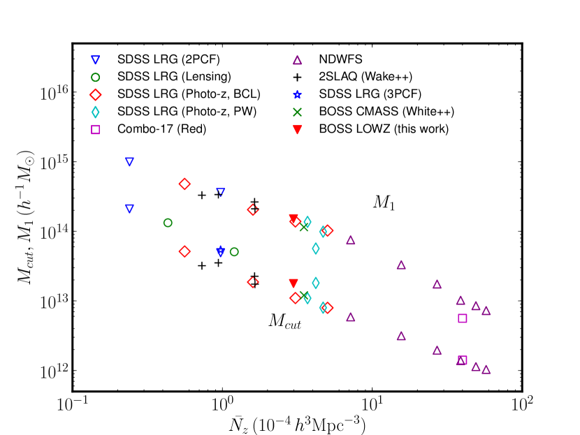
Figure 11 compares our measurements of HOD parameters $M_{cut}$ and $M_{1}$ versus galaxy number density, $\bar{{N}_{z}}$, with other studies from the literature. The HOD parameter estimates shown in this plot are taken from studies covering a range of redshifts, sample selection, spectroscopic and photometric catalogs, measurement techniques, HOD fitting methods, and survey volumes. Our results fit with the general trend of $M_{cut}$ and $M_{1}$ decreasing for higher $\bar{{N}_{z}}$. The compilation of different datasets was used in Brown et al. (2008), White et al. (2011) and Nuza et al. (2012). This result is consistent with the observation that galaxy number density is a rough proxy for the survey’s luminosity or stellar mass limit (e.g., Tinker et al., 2005; Zheng et al., 2005; Zehavi et al., 2011). For future reference, this data is also compiled in Table 4.

6 Conclusions

We have described the clustering properties of $\sim 80,000$ BOSS LOWZ galaxies from the SDSS DR9 sample. Our measurements, fitting procedure, and mock catalogs provide the following properties of this sample:

• When working with the LOWZ catalog, we recommend that approximately the first year’s data should not be included in uniform samples because it was acquired with a shallower selection function. We give a description of how to restrict the sample to the correct targets. We incorporate data from SDSS Legacy to provide about one third of our redshifts, and provide a description of how to include these data when generating large scale structure catalogs.

• The clustering of the NGC and SGC samples differ by less than $1\sigma$, even though the south has a $\sim 10\%$ higher number density because of variations in photometry. We present correlation function and fitted parameter values for the Full NGC+SGC sample and for both the NGC and SGC separately.

• The LOWZ sample has a higher correlation function amplitude ($r_{0}\sim 8.9$), but a similar bias ($b\sim 2.0$) compared to the higher redshift CMASS sample.

• The best-fit and mean HOD both result in a higher average host halo mass ($5.2\times 10^{13}h^{-1}M_{\odot}$) and steeper mass cutoff for the LOWZ sample compared to the CMASS sample, but well within the range of similar photometric galaxy samples from SDSS I/II.

• Our HOD fits result in a satellite fraction of $\sim 11\%$ for the LOWZ sample.

• The LOWZ sample is broadly consistent with being passively evolved analogs of a subset of the higher redshift CMASS sample.

7 Acknowledgments

Funding for SDSS-III has been provided by the Alfred P. Sloan Foundation, the Participating Institutions, the National Science Foundation, and the U.S. Department of Energy Office of Science. The SDSS-III web site is http://www.sdss3.org/.

SDSS-III is managed by the Astrophysical Research Consortium for the Participating Institutions of the SDSS-III Collaboration including the University of Arizona, the Brazilian Participation Group, Brookhaven National Laboratory, University of Cambridge, Carnegie Mellon University, University of Florida, the French Participation Group, the German Participation Group, Harvard University, the Instituto de Astrofisica de Canarias, the Michigan State/Notre Dame/JINA Participation Group, Johns Hopkins University, Lawrence Berkeley National Laboratory, Max Planck Institute for Astrophysics, Max Planck Institute for Extraterrestrial Physics, New Mexico State University, New York University, Ohio State University, Pennsylvania State University, University of Portsmouth, Princeton University, the Spanish Participation Group, University of Tokyo, University of Utah, Vanderbilt University, University of Virginia, University of Washington, and Yale University.

This work was supported in part by the facilities and staff of the Yale University Faculty of Arts and Sciences High Performance Computing Center, the National Energy Research Scientific Computing Center, the Shared Research Computing Services Pilot of the University of California, and the Laboratory Research Computing project at Lawrence Berkeley Laboratory.

Appendix A HOD parameters

The central galaxy occupation function in Eq. 12 allows for a log-normal scatter between galaxy luminosity and halo mass with logarithmic dispersion $\sigma$, so that the occupation of central galaxies rises smoothly from zero to one. The satellite occupation function of Eq. 13 is a power-law of slope $\alpha$ smoothly truncated at low halo masses, normalized by the mass $M_{1}$ at which halos have approximately one satellite on average. The parameter $\kappa$ allows different cutoffs in the central and satellite occupations, and it ensures that the normalization of the satellite occupation is not driven artificially by the behaviour of low-occupation halos. Occupation functions of this form provide a good fit to the theoretically predicted occupations of galaxy samples limited by stellar mass or luminosity (Kravtsov et al., 2004; Zheng et al., 2005). Our choice of HOD represents a step function with a lower mass threshold for the number of centrals (Eq. 12), smoothed out and increasing slowly to a probability of 1 over some range (the complementary error function). Similarly, as we expect the number of satellites (Eq. 13) to increase at high halo mass, we assume a power law for the number of satellites, with a minimum mass cutoff ($\kappa M_{cut}$) to prevent small halos from having satellites. Because of the color selection and the modest dependence of luminosity threshold on redshift in the BOSS LOWZ sample, we may expect the dispersion $\sigma$ to be somewhat larger than it would be for a sharply thresholded sample. See, e.g. Berlind & Weinberg (2002); Hamana et al. (2004); Zehavi et al. (2005a); Zheng et al. (2005); Zheng, Coil & Zehavi (2007); Wake et al. (2008) for other choices of HOD parameterization, some of which are analogous to ours.

As a rough guideline, the parameters affect the resulting HOD, and thus the correlation function in the following ways. $M_{cut}$ determines the characteristic minimum mass of halos in which a galaxy is allowed, and thus affects the overall amplitude of the correlation function, with smaller values of $M_{cut}$ resulting in a lower amplitude. The quantity $\sigma$ changes the shape of the “central galaxy probability function”, with smaller $\sigma$ resulting in fewer galaxies populating lower mass halos with lower large-scale bias, and thus a higher correlation function amplitude on large scales. $M_{1}$ affects the number of satellites, with smaller $M_{1}$ producing more satellites, and thus a higher amplitude for the correlation function overall, and a steeper slope at small radii. Increasing $\alpha$ increases the number of satellites, adding power on small scales, and affecting the one-halo/two-halo transition. Varying $\kappa$ has a small effect, tuning the mass at which satellites are allowed and slightly altering the small-scale correlation function. These parameters have some degeneracy, with $\sigma$ and $M_{cut}$, and $\alpha$ and $M_{1}$ positively correlated, and $M_{1}$ and $M_{cut}$ negatively correlated; we find little dependence on $\kappa$ within the range we sample, $0<\kappa<3$. Other studies that explore the relation of the HOD parameters with the resulting correlation function include Berlind & Weinberg (2002); Zheng et al. (2009); Watson, Berlind & Zentner (2011).

Figure 12: Variation of the correlation function and HOD as individual HOD parameters change. From the top panel to the bottom panel, the parameter that is varied is $M_{1}$, $M_{cut}$, $\sigma$, $\kappa$, $\alpha$. The thick black line is the NGC correlation function described in this paper.

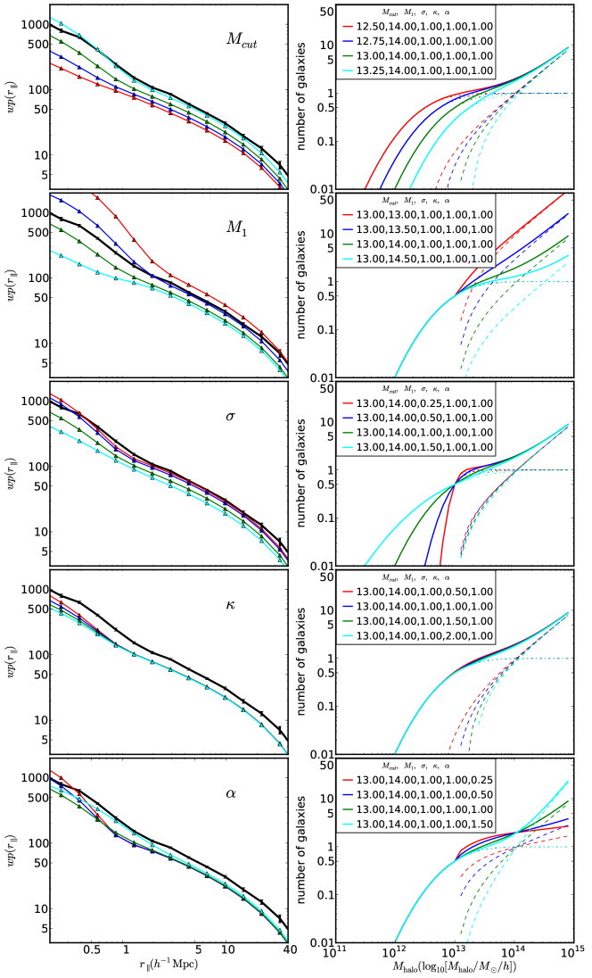
Figure 12 shows how the correlation function, $w_{p}(r_{p})$, and the satellite and central halo functions vary as each individual HOD parameter is changed over a range of reasonable values. Each panel includes one set of curves with the values $M_{1}=13.00$, $M_{cut}=14.00$, $\sigma=1.00$, $\kappa=1.00$, $\alpha=1.00$ as a fiducial. The degeneracies in the correlation functions between the parameters are visible, as well as the effects that each has on the shape and amplitude of the resulting correlation function.

The values of $M_{cut}$ and $M_{1}$ from previous studies used in Figure 11 are given in Table 4.

Table 4: $M_{cut}$ and $M_{1}$ versus $\bar{N}_{z}$ from various studies

$\bar{N}_{z}$	$\log_{10}M_{cut}$	$\log_{10}(M_{1})$	Sample
9.730E-5	13.6907	14.5587	0
2.400E-5	14.3217	14.9967	0
1.200E-4	13.7055	0.0000	1
4.330E-5	14.1224	0.0000	1
9.730E-5	13.7328	0.0000	7
9.400E-5	13.5464	14.5278	6
1.640E-4	13.3540	14.4215	6
5.753E-3	12.0150	12.8610	5
4.916E-3	12.0560	12.9310	5
3.888E-3	12.1420	13.0090	5
2.708E-3	12.2920	13.2420	5
1.562E-3	12.4990	13.5190	5
7.171E-4	12.7700	13.8770	5
5.030E-4	12.9008	14.0108	2
3.070E-4	13.0408	14.1408	2
1.600E-4	13.2708	14.3108	2
5.600E-5	13.7108	14.6808	2
3.700E-4	13.0390	14.1350	3
4.700E-4	12.9029	13.9942	3
4.200E-4	13.2578	13.7528	3
7.300E-5	13.5057	14.5182	6
1.650E-4	13.2408	14.3228	6
4.000E-3	12.1500	12.7500	4
3.500E-4	13.0800	14.0600	8
2.981E-4	13.2500	14.1800	9

Sample numbers refer to the following works: 0: SDSS LRG (2PCF), Zheng et al. (2009); 1: SDSS LRG (Lensing), Mandelbaum et al. (2006); 2: SDSS LRG (Photo-z, BCL), Blake, Collister & Lahav (2008); 3: SDSS LRG (Photo-z, PW), Padmanabhan et al. (2009); 4: Combo-17 (Red), Phleps et al. (2006); 5: NDWFS, Brown et al. (2008); 6: 2SLAQ (Wake++), Wake et al. (2008); 7: SDSS LRG (3PCF), Kulkarni et al. (2007); 8: BOSS CMASS (White++), White et al. (2011); 9: this work.

References

- Aihara et al. (2011) Aihara H. et al., 2011, ApJS, 193, 29
- Amanullah et al. (2010) Amanullah R. et al., 2010, ApJ, 716, 712
- Anderson et al. (2012) Anderson L. et al., 2012, ArXiv e-prints
- Bennett et al. (2003) Bennett C. L. et al., 2003, ApJS, 148, 1
- Benson et al. (2000) Benson A. J., Baugh C. M., Cole S., Frenk C. S., Lacey C. G., 2000, MNRAS, 316, 107
- Berlind et al. (2006) Berlind A. et al., 2006, ApJS, 167, 1
- Berlind & Weinberg (2002) Berlind A. A., Weinberg D. H., 2002, ApJ, 575, 587
- Blake, Collister & Lahav (2008) Blake C., Collister A., Lahav O., 2008, MNRAS, 385, 1257
- Brown et al. (2008) Brown M. J. I. et al., 2008, ApJ, 682, 937
- Cannon et al. (2006) Cannon R. et al., 2006, MNRAS, 372, 425
- Carlson & White (2010) Carlson J., White M., 2010, ApJS, 190, 311
- Colless et al. (2003) Colless M. et al., 2003, ArXiv Astrophysics e-prints
- Cooray & Sheth (2002) Cooray A., Sheth R., 2002, Phys. Rep., 372, 1
- Davis et al. (1985) Davis M., Efstathiou G., Frenk C. S., White S. D. M., 1985, ApJ, 292, 371
- Davis & Peebles (1983) Davis M., Peebles P. J. E., 1983, ApJ, 267, 465
- de Vaucouleurs (1948) de Vaucouleurs G., 1948, Annales d’Astrophysique, 11, 247
- Doi et al. (2010) Doi M. et al., 2010, AJ, 139, 1628
- Eisenstein et al. (2001) Eisenstein D. J. et al., 2001, AJ, 122, 2267
- Eisenstein et al. (2011) —, 2011, AJ, 142, 72
- Eisenstein et al. (2005) —, 2005, ApJ, 633, 560
- Freeman (1970) Freeman K. C., 1970, ApJ, 160, 811
- Fry (1996) Fry J., 1996, ApJ, 461, L65
- Fukugita et al. (1996) Fukugita M., Ichikawa T., Gunn J. E., Doi M., Shimasaku K., Schneider D. P., 1996, AJ, 111, 1748
- Gunn et al. (1998) Gunn J. E. et al., 1998, AJ, 116, 3040
- Gunn et al. (2006) —, 2006, AJ, 131, 2332
- Guo, Zehavi & Zheng (2011) Guo H., Zehavi I., Zheng Z., 2011, ArXiv e-prints
- Hamana et al. (2004) Hamana T., Ouchi M., Shimasaku K., Kayo I., Suto Y., 2004, MNRAS, 347, 813
- Hastings (1970) Hastings W. K., 1970, Biometrika, 57, 97
- Howlett et al. (2012) Howlett C., Lewis A., Hall A., Challinor A., 2012
- Kaiser (1987) Kaiser N., 1987, MNRAS, 227, 1
- Kessler et al. (2009) Kessler R. et al., 2009, ApJS, 185, 32
- Komatsu et al. (2011) Komatsu E. et al., 2011, ApJS, 192, 18
- Kowalski et al. (2008) Kowalski M. et al., 2008, ApJ, 686, 749
- Kravtsov et al. (2004) Kravtsov A. V., Berlind A. A., Wechsler R. H., Klypin A. A., Gottlöber S., Allgood B., Primack J. R., 2004, ApJ, 609, 35
- Kroupa (2001) Kroupa P., 2001, MNRAS, 322, 231
- Kulkarni et al. (2007) Kulkarni G. V., Nichol R. C., Sheth R. K., Seo H.-J., Eisenstein D. J., Gray A., 2007, MNRAS, 378, 1196
- Lampeitl et al. (2010) Lampeitl H. et al., 2010, MNRAS, 401, 2331
- Landy & Szalay (1993) Landy S. D., Szalay A. S., 1993, ApJ, 412, 64
- Lewis, Challinor & Lasenby (2000) Lewis A., Challinor A., Lasenby A., 2000, Astrophys. J., 538, 473
- Lupton et al. (2001) Lupton R., Gunn J. E., Ivezić Z., Knapp G. R., Kent S., 2001, in ASP Conf. Ser. 238: Astronomical Data Analysis Software and Systems X, Harnden Jr. F. R., Primini F. A., Payne H. E., eds., pp. 269–+
- Mandelbaum et al. (2006) Mandelbaum R., Seljak U., Kauffmann G., Hirata C. M., Brinkmann J., 2006, MNRAS, 368, 715
- Maraston et al. (2012) Maraston C. et al., 2012, ArXiv e-prints
- Maraston et al. (2009) Maraston C., Strömbäck G., Thomas D., Wake D., Nichol R. C., 2009, MNRAS, 394, L107
- Metropolis et al. (1953) Metropolis N., Rosenbluth A. W., Rosenbluth M. N., Teller A. H., Teller E., 1953, J. Chem. Phys., 21, 1087
- Navarro, Frenk & White (1996) Navarro J. F., Frenk C. S., White S. D. M., 1996, ApJ, 462, 563
- Nuza et al. (2012) Nuza S. E. et al., 2012, ArXiv e-prints
- Padmanabhan (inprep) Padmanabhan, N. e. a., inprep
- Padmanabhan et al. (2008) Padmanabhan N. et al., 2008, ApJ, 674, 1217
- Padmanabhan et al. (2009) Padmanabhan N., White M., Norberg P., Porciani C., 2009, MNRAS, 397, 1862
- Peacock & Smith (2000) Peacock J. A., Smith R. E., 2000, MNRAS, 318, 1144
- Peebles (1980) Peebles P. J. E., 1980, The large-scale structure of the universe, Peebles, P. J. E., ed.
- Phleps et al. (2006) Phleps S., Peacock J. A., Meisenheimer K., Wolf C., 2006, A&A, 457, 145
- Pier et al. (2003) Pier J. R., Munn J. A., Hindsley R. B., Hennessy G. S., Kent S. M., Lupton R. H., Ivezić Ž., 2003, AJ, 125, 1559
- Ross et al. (2011) Ross A. J. et al., 2011, MNRAS, 417, 1350
- Schlafly & Finkbeiner (2011) Schlafly E. F., Finkbeiner D. P., 2011, ApJ, 737, 103
- Schlafly et al. (2010) Schlafly E. F., Finkbeiner D. P., Schlegel D. J., Jurić M., Ivezić Ž., Gibson R. R., Knapp G. R., Weaver B., 2010, ApJ, 725, 1175
- Schlegel, White & Eisenstein (2009) Schlegel D., White M., Eisenstein D., 2009, in Astronomy, Vol. 2010, astro2010: The Astronomy and Astrophysics Decadal Survey, pp. 314–+
- Schlegel, Finkbeiner & Davis (1998) Schlegel D. J., Finkbeiner D. P., Davis M., 1998, ApJ, 500, 525
- Scoccimarro (2004) Scoccimarro R., 2004, Phys. Rev. D, 70, 083007
- Scoccimarro et al. (2001) Scoccimarro R., Sheth R. K., Hui L., Jain B., 2001, ApJ, 546, 20
- Seljak (2000) Seljak U., 2000, MNRAS, 318, 203
- Seljak (2001) —, 2001, MNRAS, 325, 1359
- Skibba et al. (2009) Skibba R. et al., 2009, MNRAS, 399, 966
- Skibba et al. (2006) Skibba R., Sheth R. K., Connolly A. J., Scranton R., 2006, MNRAS, 369, 68
- Skibba & Sheth (2009) Skibba R. A., Sheth R. K., 2009, MNRAS, 392, 1080
- Smith et al. (2002) Smith J. et al., 2002, AJ, 123, 2121
- Sollerman et al. (2009) Sollerman J. et al., 2009, ApJ, 703, 1374
- Strauss et al. (2002) Strauss M. et al., 2002, AJ, 124, 1810
- Tinker, Weinberg & Zheng (2006) Tinker J. L., Weinberg D. H., Zheng Z., 2006, MNRAS, 368, 85
- Tinker et al. (2005) Tinker J. L., Weinberg D. H., Zheng Z., Zehavi I., 2005, ApJ, 631, 41
- Tojeiro et al. (2012) Tojeiro R. et al., 2012, ArXiv e-prints
- Tojeiro & Percival (2010) Tojeiro R., Percival W. J., 2010, MNRAS, 405, 2534
- Tojeiro & Percival (2011) —, 2011, MNRAS, 417, 1114
- van Daalen, Angulo & White (2012) van Daalen M. P., Angulo R. E., White S. D. M., 2012, ArXiv e-prints
- Wake et al. (2008) Wake D. et al., 2008, MNRAS, 387, 1045
- Watson, Berlind & Zentner (2011) Watson D. F., Berlind A., Zentner A. R., 2011, ApJ, 738, 22
- White (2001) White M., 2001, MNRAS, 321, 1
- White et al. (2011) White M. et al., 2011, ApJ, 728, 126
- White, Hernquist & Springel (2001) White M., Hernquist L., Springel V., 2001, ApJ, 550, L129
- White et al. (2007) White M., Zheng Z., Brown M. J. I., Dey A., Jannuzi B. T., 2007, ApJ, 655, L69
- York et al. (2000) York D. G. et al., 2000, AJ, 120, 1579
- Zehavi et al. (2002) Zehavi I. et al., 2002, ApJ, 571, 172
- Zehavi et al. (2005a) —, 2005a, ApJ, 621, 22
- Zehavi et al. (2004) —, 2004, ApJ, 608, 16
- Zehavi et al. (2011) —, 2011, ApJ, 736, 59
- Zehavi et al. (2005b) —, 2005b, ApJ, 630, 1
- Zheng et al. (2005) Zheng Z. et al., 2005, ApJ, 633, 791
- Zheng, Coil & Zehavi (2007) Zheng Z., Coil A. L., Zehavi I., 2007, ApJ, 667, 760
- Zheng et al. (2009) Zheng Z., Zehavi I., Eisenstein D. J., Weinberg D. H., Jing Y. P., 2009, ApJ, 707, 554
- Zu et al. (2008) Zu Y., Zheng Z., Zhu G., Jing Y. P., 2008, ApJ, 686, 41