Is the Weibull distribution really suited for wind statistics modeling and wind power evaluation?
Abstract
Wind speed statistics is generally modeled using the Weibull distribution. This distribution is convenient since it fully characterizes analytically with only two parameters (the shape and scale parameters) the shape of distribution and the different moments of the wind speed (mean, standard deviation, skewness and kurtosis). This distribution is broadly used in the wind energy sector to produce maps of wind energy potential. However, the Weibull distribution is based on empirical rather than physical justification and might display strong limitations for its applications. The philosophy of this article is based on the modeling of the wind components instead of the wind speed itself. This provides more physical insights on the validity domain of the Weibull distribution as a possible relevant model for wind statistics and the quantification of the error made by using such a distribution. We thereby propose alternative expressions of more suited wind speed distribution.
Keywords:
Surface wind, Wind statistics, Wind energy, Weibull distribution, Rayleigh distribution, Rice distribution, Superstatistics.
1 Introduction
Understanding and modeling wind speed statistics is a key for a better understanding of atmospheric turbulence and diffusion and for use in such practical applications as air quality and pollution transport modeling, estimation of wind loads on buildings, prediction of atmospheric or space probe and missile trajectory and wind power analysis. In the context of wind energy production, it is necessary to characterize the wind in a planned wind turbine farm location, in order to calculate the optimal cut-in and cut-out speed and the likely power output of a given wind turbine (Drobinski 2012). This is done using the distribution of wind speed . In particular, a key parameter to describe wind power is the average wind power produced by a wind turbine,
| (1) |
where is the area of the flow, is the density of the fluid, is the coefficient of power of the wind turbine which measures how efficiently the wind turbine converts the energy in the wind into electricity, is the energy pattern, and is the third moment of the distribution. In order to describe the wind energy potential independently of the turbine shapes, observed histograms are fitted to the Weibull distribution, defined as follows,
| (2) |
where is the wind speed, is the shape parameter and is the scale parameter of the distribution. In this case, and , where is the Gamma function. The Weibull distribution is thus an extremely used paradigm to model wind statistics (e.g. Justus et al. 1976, 1978, Seguro and Lambert 2000, Cook 2001, Weisser 2003, Ramírez and Carta 2005) because it can be easily fit after estimating the parameters and and it produces analytical expressions for the different moments and the wind power. However, its use is purely empirical and there is a lack of physical background justifying the use of the Weibull distribution to model wind statistics. Besides, the validity of the description of wind statistics by a Weibull distribution is not clearly established. Therefore, the estimated wind potential might be systematically mis-estimated.
In this paper, we use meteorological data to show that, in some locations with particularly high wind potential but wind anisotropy, wind statistics is not well described by the Weibull distribution, thus leading to a systematic under-estimation of wind power, up to . We then provide physical insights for the origin of such a discrepancy. To this end, we consider wind velocity as a bivariate distribution of the two orthogonal (e.g. north-south and east-west) wind components and we compute it analytically in the simple case of normal distributions. This allows us to derive a Rayleigh-Rice super-statistical distribution, which is better suited than the Weibull distribution to describe real data in locations where the wind is not isotropic. Finally, we generalize this approach to the case of isotropic wind with non-Gaussian wind components, where the Weibull distribution better describes the meteorological data.
2 Observations
In this study, we use wind measurements collected between December, 28st 2006 and March 20th 2008 at 10 m height from 4 surface weather stations at different locations in France (Fig. 1). Among the 4 stations, 3 are operational weather stations from the French national weather service Météo-France and one is the research observatory (Haeffelin et al. 2005). While the wind components from the 3 operational weather stations are recorded every three hours, the SIRTA observatory data is recorded every minute. The SIRTA observatory is located at Palaiseau, 20 km south of Paris, France. The site is in a suburban area. We use the wind measurements on a tower surrounded by different types of surface, i.e. close and distant forest, buildings and an open field sector (Drobinski et al. 2006, Barthlott et al. 2007, Fesquet et al. 2009).
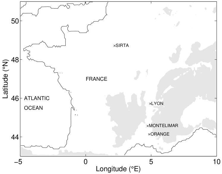
The Météo-France stations are located in a much more complex environment with elevated mountain ridges. In this region, frequent channelled wind can persist for several days. The strongest and most frequent channeled valley wind is the mistral, which blows from the north/north-west in the Rhône valley, separating the French Alps (highest elevation 4807 m) to the east from the Massif Central (highest elevation 1885 m) to the west by a gap 200 km long and 60 km wide (Fig. 1) (Drobinski et al. 2005). It occurs when a synoptic northerly flow impinges on the Alpine range. As the flow experiences channeling, it is substantially accelerated and can extend offshore over horizontal ranges exceeding few hundreds of kilometers (Salameh et al. 2007, Lebeaupin-Brossier and Drobinski 2009). The mistral occurs all year long but exhibits a seasonal variability either in speed and direction, or in its spatial distribution (Mayencon 1982, Orieux and Pouget 1984, Guénard et al. 2005, Guénard et al. 2006). During summer, the mistral shares its occurrence with a northerly land breeze and southerly sea-breeze (e.g. Bastin and Drobinski, 2005, 2006; Drobinski et al., 2006, 2007), which can also be channelled in the nearby valleys (Bastin et al., 2005) or interact with the mistral (Bastin et al., 2006). In such region, accounting for such persistent wind systems for modeling the wind speed statistics is thus mandatory.
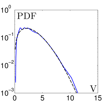
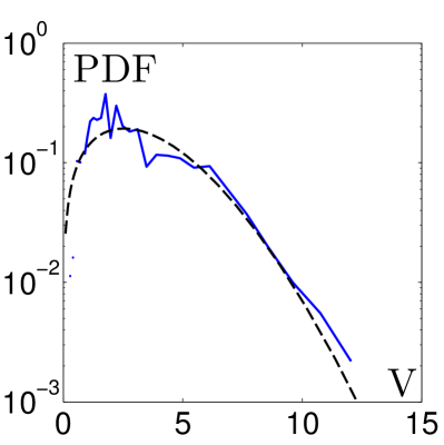
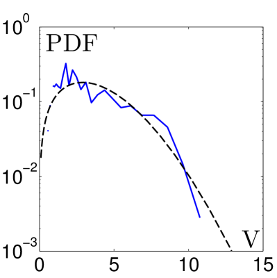
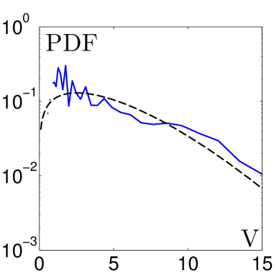
Figure 2 shows the probability density functions (PDF) of the wind speed at the SIRTA observatory, Lyon, Montélimar and Orange and their fits by a Weibull distribution.
(a) (b)
(c) (d)
First, while the Weibull distribution is an accurate statistical model for the wind speed distribution at SIRTA (Fig. 2a), it poorly describes wind distributions measured at the 3 weather stations located in complex terrain (Fig. 2b-d). Table 1 compares the wind power computed from the wind speed observations and that is estimated from the Weibull distribution best fit using Eq. (1). The parameters and are also indicated. At the SIRTA observatory, the wind power estimated from Eq. (1) is accurate up to %. It is obtained for a value . The Weibull distribution describes fairly well the wind distribution at SIRTA, which we stress, is located in a fairly flat terrain. Yet, the difference between the data and the fit is not random fluctuations: there are small systematic differences occurring at large ( m.s-1) and at low ( m.s-1) wind speed values.
-
Stations Power Data Weibull Elliptic Rayleigh-Rice [;] [;] [] SIRTA 1.63 1.59 1.48 1.13 [1.71;3.58] [2.64;2.64] [0.05] Lyon 2.26 2.22 2.17 2.26 [1.76;4.11] [2.33;3.54] [0.297] Montelimar 2.75 2.55 2.53 2.74 [1.82;4.48] [2.65;3.73] [0.230] Orange 7.71 6.78 6.75 7.59 [1.45;5.69] [2.93;5.53] [0.510]
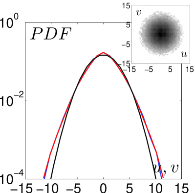
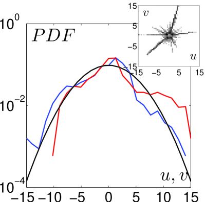
In contrast, at Montélimar and Orange, Weibull fit quality drops (Fig. 2c-d), and systematically underestimates the right tail of the distributions. As a result, the power is systematically underestimated by % and % (Table 1). To the best of our knowledge, this systematic discrepancy has not been reported in the existing literature, although it is a major issue for wind power resource evaluation. At Lyon, Montélimar and Orange, the observed distributions display complex shapes instead of a smooth and regular shape as would be expected when fitting with a Weibull distribution. As opposed to the regular shape of wind speed and the surrounding topography at SIRTA, the complexity of the distributions in the Rhône valley might originate in the complexity of the surrounding topography. For a deeper insight of the differences between observed wind speed distributions and the commonly used Weibull distribution, the distribution of the wind components are now investigated (Fig. 3). At the SIRTA observatory (Fig. 3a), the zonal and meridional wind components have the same symmetrical distributions with zero mean and equal width: the wind is isotropic. In addition, the distributions of wind components have larger tails than Gaussian.
(a) (b)
(c) (d)
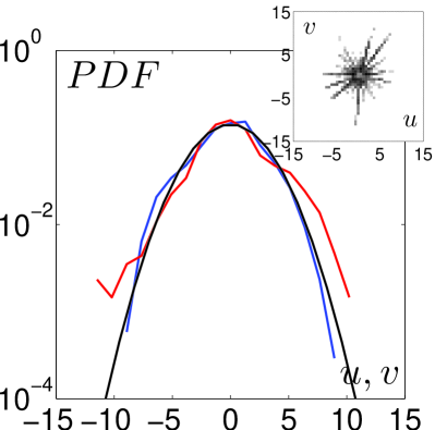
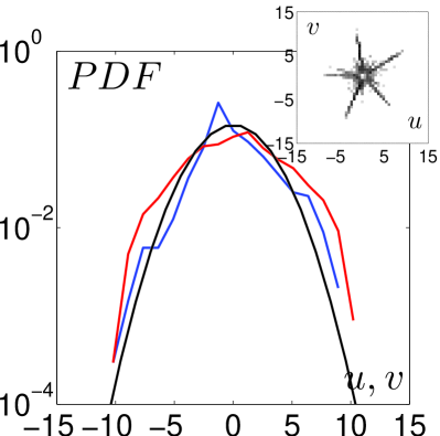
At Lyon (Fig. 3b), at the entrance of the Rhône valley, the PDF of the zonal wind component is still symmetrical with almost zero mean and has a Gaussian shape. The PDF of the meridional wind component is fairly symmetrical for values below 5 m s-1 but is skewed for the strongest values. Also the width of the meridional wind PDF is larger than that of the zonal wind. At Montélimar and Orange, none of the wind component PDFs look like Gaussian distribution and the meridional wind PDF become significantly larger than the PDF of the zonal wind. This shows evidence of the channelled nature of the wind by the north-south oriented Rhône valley (Salameh et al. 2009). For low winds, the PDFs of the zonal and meridional components are more similar, evidencing a less efficient impact of the valley flanks to orientate the wind.
The two wind components may however be correlated. The insets of Fig. 3 show the joint distribution of the two wind components at SIRTA observatory, Lyon, Montélimar and Orange. At the SIRTA observatory, the rather flat terrain produces an isotropic wind statistics (i.e. the wind blows in all directions) with no correlation between the two components (i.e. the joint distribution displays a circular shape). Conversely, the joint distributions at Lyon, Montélimar and Orange display strongly correlated wind components in specific directions. The main directions correspond to the north-south orientation of the Rhône valley.
To conclude on the observations, it appears that at SIRTA and Lyon, while the Weibull function fits better wind speed distributions, the wind components are less anisotropic. Therefore, it seems that isotropy is crucial for the Weibull description to be valid. In the following, despite the fact that none of the observed distributions is Gaussian, we shall focus on anisotropic bivariate distribution to understand the effect of anisotropy on the resulting wind speed distribution.
3 From Gaussian to super-statistical Gaussian wind components
3.1 The Rayleigh distribution
The very first approach to model anisotropy is to consider a bivariate distribution of Gaussian wind components with means and , and variances and and finite cross-correlation . After a change of variable, , , the resulting joint distribution is a bivariate elliptical distribution with variances and without correlation. In the case (Crutcher and Baer 1962),
| (4) |
Applying the usual transformation from Cartesian to polar coordinates (,), and integrating over the angle , the joint PDF for and is (Chew and Boyce 1962):
| (5) |
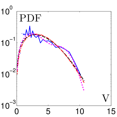
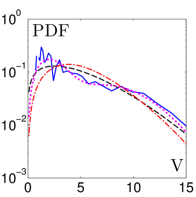
with and , and where is the modified Bessel function of the first kind and zero order. When the variance are equal , so and Eq. (5) is the Weibull distribution with parameter , which is the Rayleigh distribution. When comparing the elliptical normal joint distribution with data, (Table 1 and Fig. 4), it is worse than a fit by the Weibull distribution. Despite the fact taking account of anisotropy of wind components modifies the tail of the distributions, the Gaussian approximation is too crude to model wind speed components. However, using Gaussian distributions is a powerful approach because analytic calculation can be performed.
(a) (b)
3.2 The Rice distribution
As a second order approximation and for the sake of simplicity, we now consider the case of elliptic distributions with non zero mean and and equal variances . equal variances for the two wind components. Thus, we obtain
| (6) |
with . The distribution in Eq. (6) is called the Rice distribution and is the order modified Bessel function of the first kind.
3.3 The Rayleigh-Rice distribution
The key assumption we do in the following is that, in the Rhône valley area, there are two regimes: (i) random flow: the wind components have zero means and same variances, and the Rayleigh distribution describes well the wind speed statistics; (ii) channeled flow: the wind components have different means, and the Rice distribution describes well the wind speed statistics. The resulting distribution is a sum of the distribution (i) and (ii) conditioned to the absence and presence of the channeled flow occurrence. In other words, in the long-term, the wind system is described as the superposition of different local dynamics at different intervals that has been coined by Beck and Cohen (2003) as superstatistics or statistics of statistics. This yields, for one wind component, for instance the zonal wind, (similar expression would arise for the meridional component, ):
| (7) |
In the case of the two regimes scenario, is bimodal,
| (8) |
where is the Dirac function and is here the weight corresponding to channeled flow events occurrence. The PDF of , is thus a combination of a Rayleigh distribution (corresponding to ) and a Rice distribution. Such a method has been used to include in wind statistics modeling the contribution of zero wind speed (Tackle and Brown 1978, Tuller and Brett 1983). As a result we obtain the Rayleigh-Rice distribution:
| (9) |
where is the normalization factor.
When comparing to data, the weighted Rayleigh-Rice function provides a much better fit (Fig. 4) and estimates much better the wind power (Table 1) than the Weibull distribution. We indeed obtain less than relative error for all locations and even less than in Montélimar. Table 1 shows that the weighted Rayleigh-Rice function gives by far the best estimate of the wind power at Lyon, Montélimar and Orange. The values of correspond very accurately to the probability of occurrence of the dominating mistral situations (Orieux and Pouget 1984). Thus, taking account of the existence of regimes in regions where mountain environments is a fruitful approach to quantify wind speed statistics and to estimate wind power potential.
4 Non-Gaussian distributions
4.1 Super-statistics
Figure 3 shows that at SIRTA, where the environment is much less complex than at the 3 other weather stations, the PDFs of the two wind components are not accurately predicted by a normal distribution and displays heavy tails. Such heavy tails illustrate the departure of the wind component PDFs from the normal distribution model. We show here that super-statistics can help for the understanding the non-Gaussian shape. Since both wind components at the SIRTA station have very close statistical properties (Fig. 3a), for the sake of concision, we will focus on one component, , throughout this section.
The large tails of the wind component distributions at SIRTA (Fig. 3a) originate in the transient nature of the wind. Meteorological conditions indeed change on several time-scales (day, anticyclones duration, season). For instance, the strongest wind being typically recorded in the winter, whereas in summer, long-lasting anticyclonic conditions give lower wind speeds. This induces a change of the statistical properties (e.g. wind component variance) on several entangled time scales. Here, we model this by assuming Gaussian shape of wind distribution, but with changing standard deviation, . The super-statistics of the wind components can be derived as follows (Rizzo and Rapisarda 2004):
| (10) |
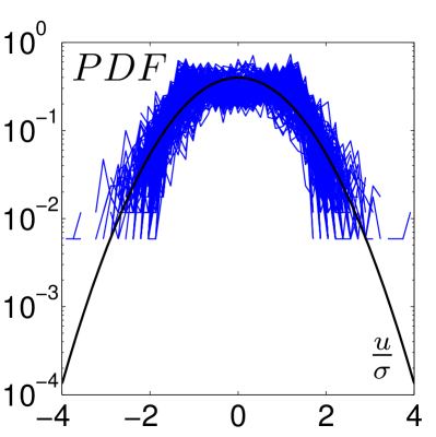
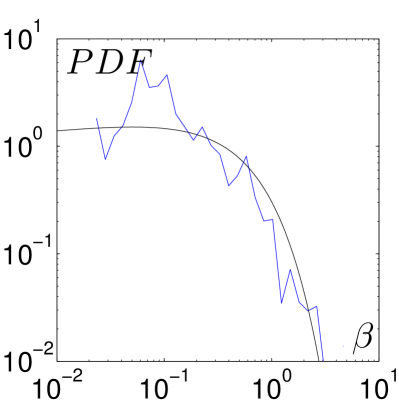
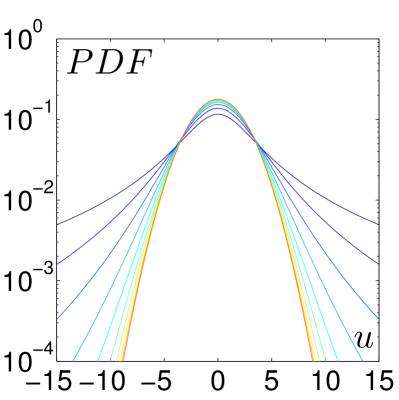
where is the probability distribution of the fluctuating variable . Figure 5a shows the distributions of short samples of wind component speed measured at the SIRTA observatory, rescaled by their standard deviation, , computed over 4 hr time periods.
(a) (b)
(c) (d)
We see that the distributions of wind component velocity acquired during short time samples is well rescaled by its standard deviation. We can therefore assume the wind component distributions to be
| (11) |
Figure 5b shows the distribution of each sample standard deviation and its fit by a Gamma distribution. We see that the distribution of is consistent with a Gamma distribution, of parameters and :
| (12) |
where is the Gamma function. Hence, combining it to Eq. (10), we obtain
| (13) |
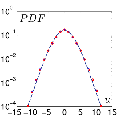
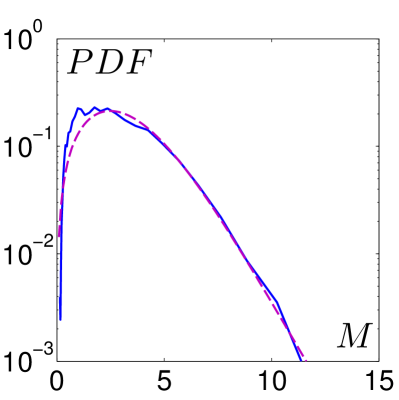
where is the Euler integral of the first kind. This distribution is called the generalized Boltzmann factor. It has been obtained when attempting to generalize the entropy definition (Tsallis 1988, Beck and Cohen 2003). The distributions modeled with Eq. (13) display heavy power law tails reminiscent of rare events (Fig. 5c). Unfortunately, our data has not enough statistics to observe such rare events and we can not compare the tails of the distribution (Fig. 5d). Yet, note that the central part of the observed distributions matches very well the distributions of Eq. (13) (Fig. 5d).
We now turn to wind speed distribution, which is at stake for wind energy. For the sake of simplicity, we assume that the components and are independent statistically. Besides, we had previously observed that: (i) there is no correlation between and (Fig. 3a-inset); (ii) and have similar statistics, i.e. both components are described by the same and . Therefore the wind speed distribution is obtained by computing the joint distribution in radial coordinates and integrated over the angle. Therefore, we obtain
| (14) |
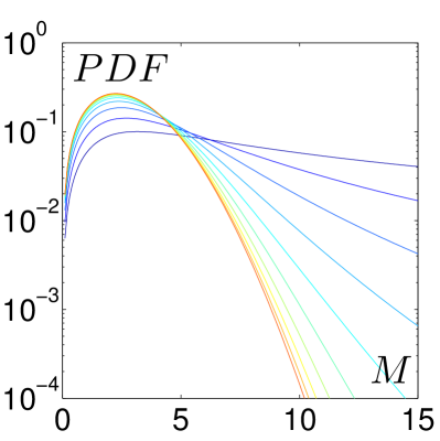
where is the Euler integral of the first kind and is the hypergeometric function. Again, this yields a heavy tail distribution (Fig. 6a), but for the set of parameters that fits the data the most (Fig. 6b), the wide tails occur for very low probability, and Eq. (14) fits very well the data.
(a) (b)
4.2 Physical origin of super-statistics: stationary solutions of stochastic differential equations
For a more in-depth analysis of the physical processes, several studies model the wind speed or its components using stochastic differential equation (SDE) (e.g. Nfaoui et al. 2004, Bernardin et al. 2009). A first order SDE for stochastic process can be written as:
| (15) |
where and are arbitrary functions and is a random function of time, often referred to as a ”noise term”. Considering the time evolution of the probability density function, , associated to the stochastic variable, , Eq. (15) can be converted into the Fokker-Planck equation,
| (16) |
If is constant, the system is said to be subject to additive noise, otherwise it is said to be subject to multiplicative noise. The stochastic processes is usually a Markov process, i.e. characterized as memoryless: the next state depends only on the current state and not on the sequence of events that preceded it. A number of authors have modeled explicitly the temporal dependence of the wind speed through Markov chain models (Youcef Ettoumi et al. 2003, Nfaoui et al. 2004, Shamshad et al. 2005, Fawcett and Walshaw 2006a, Fawcett and Walshaw 2006b). Interestingly, it turns out that the distribution of Eq. (13) is also the stationary solution of Eq. (16), with and , where and are constants governing the strength of the multiplicative (first term) and additive (second term) noise. The relations between , and the parameters of Eq. (11) are:
| (19) |
The multiplicative and additive noise terms can be physically interpreted as an interplay between turbulence, chaotic atmospheric variability and the mean wind (Bernardin et al. 2009). In the case of non-multiplicative noise, , the strength of the noise does not depend on the mean wind and the resulting stationary distribution is Gaussian. Conversely, the multiplicative stochastic process, used to model wind stress over the ocean by Sura and Gille (2003), makes the link between the wind variability and its mean state and induces a stationary power-law distribution (Sakaguchi 2001). Yet, as the observed wind component distributions are narrower than power-laws, this multiplicative stochastic model is crude to describe them. Finally, besides the rather accurate but empirical fit of the Weibull distribution to measured wind speed distribution, is there thus a physical reason to model wind speed statistics with a Weibull distribution? In order to address this question, a first step might be to consider a SDE with and (Queirós 2008). Indeed, this yields the joint PDF for wind speed, and direction, ,
| (22) |
with the corresponding normalization factor. Despite the fact that Eq. (22) can not be integrated with respect to between 0 and because of integration singularities, it shares common features with a Weibull distribution, namely the power-law and stretched-exponential with exponent . Future works will thus explore in more detail the potential of such SDE to model wind speed statistics.
5 Conclusion
The use of the Weibull distribution for wind statistics modeling and wind energy evaluation is a convenient and powerful approach. Is is however based on empirical more than physical justification and might display at times strong limitations for its application. In this article, we model the wind components instead of the wind speed itself, and thereby provide more physical insights on the validity domain of the Weibull distribution as a possible relevant model for wind statistics.
Based on wind measurements collected nearby Paris in a rather flat environment and in Southern France in the Rhône valley in a ridge and mountains environment, this article proposes different probability density functions of the wind components. This opens the path to the analysis of the applicability of the Weibull distribution as a suited model for wind statistics and the quantification of the errors on the mean wind speed and wind power arising from the use of the Weibull distribution.
This study first shows that in complex terrain, the existence of terrain induced wind system affects the surface wind distribution which does not display a Weibull shape. Modeling the wind statistics with a Weibull distribution produces errors exceeding on the wind power estimate. The combination of a Rayleigh distribution to model the “isotropic” wind and a Rice distribution to model persistent wind regimes gives excellent results for the three surface weather stations located in the Rhône valley. Combining Rayleigh and Rice distributions is equivalent to applying the recently developed super-statistics theory, which models the wind system as the superposition of different local dynamics at different intervals with different mean wind speeds. However, Rayleigh and Rice distributions assume normal distributions for the two wind components. The distributions of the wind components, even over flat terrain, however exhibit non Gaussian distribution. This can also be modeled using super-statistics theory, which assumes fluctuating variances of the two wind components, that are eventually modeled by a Gaussian distribution over a short time interval. However, this produces power-law distribution for large wind speed value which contradict observed distributions and Weibull model. This can be partly overcome by assuming the wind components to verify stochastic differential equation with multiplicative noise with power coefficient.
Parametric statistical downscaling using the Weibull distribution is often used to produce regional surface wind speed climatologies (Pryor et al. 2005). Also, this study points out the limits of the use of parametric distribution to downscale surface wind speed and advocates for non parametric statistical models (e.g. Michelangeli et al. 2009, Salameh et al. 2009, Lavaysse et al. 2012,Vrac et al. 2012).
References
References
- [1] Barthlott C, Drobinski P, Fesquet C, Dubos T and Pietras C 2007 Long-term study of coherent structures in the atmospheric surface layer Boundary-Layer Meteorol. 125 1-24
- [2] Bastin S and Drobinski P 2005 Temperature, and wind velocity oscillations along a gentle slope during sea breeze events Boundary-Layer Meteorol. 114 573-594
- [3] Bastin S, Drobinski P, Dabas A M, Delville P, Reitebuch O and Werner C 2005. Impact of the Rhône and Durance valleys on sea-breeze circulation in the Marseille area Atmos. Res. 74 303-328
- [4] Bastin S and Drobinski P 2006 Sea breeze induced mass transport over complex terrain in southeastern France: a case study Q. J. R. Meteorol. Soc. 132 405-423
- [5] Bastin S, Drobinski P, Guénard V, Caccia J L, Campistron B, Dabas A M, Delville P, Reitebuch O and Werner C 2006 On the interaction between sea breeze, and summer mistral at the exit of the Rhône valley Mon. Wea. Rev. 134 1647-1668
- [6] Beck C and Cohen, EGD 2003 Superstatistics Physica A 332 267-275
- [7] Bernardin F, Bossy M, Chauvin C, Drobinski P, Rousseau A and Salameh T 2009 Stochastic downscaling method: application to wind refinement Stoch. Env. Res. Ris. Assess. 23 851-859
- [8] Chew V and Boyce R 1962 Distribution of radial error in the bivariate elliptical normal distribution Technometrics 4 138-140
- [9] Cook P 2001 ”Discussion on modern estimation of the parameters of the Weibull wind speed distribution for wind speed energy analysis” by J.V. Seguro, T.W. Lambert Journal of Wind Engineering and Industrial Aerodynamics 89 867-869
- [10] Crutcher H L and Baer L 1962 Computations from elliptical wind distribution statistics J. Appl. Meteorol. 1 522-530
- [11] Drobinski P, Bastin S, Guénard V, Caccia J L, Dabas A M, Delville P, Protat A, Reitebuch O and Werner C 2005 Summer mistral at the exit of the Rhône valley Q. J. R. Meteorol. Soc. 131 353-375
- [12] Drobinski P, Redelsperger J L and Pietras C 2006a Evaluation of a planetary boundary layer subgrid-scale model that accounts for near-surface turbulence anisotropy Geophys. Res. Lett. 33 L23806 10.1029/2006GL027062
- [13] Drobinski P, Bastin S, Dabas A M, Delville P and Reitebuch O 2006b Variability of the three-dimensional sea-breeze structure in southeastern France: observations and evaluation of empirical scaling laws Ann. Geophys. 24 1783-1799
- [14] Drobinski P, Saïd F, Ancellet G, Arteta J, Augustin P, Bastin S, Brut A, Caccia J L, Campistron B, Cautenet S, Colette A, Coll I, Cros B, Corsmeier U, Dabas A M, Delbarre H, Dufour A, Durand P, Guénard V, Hasel M, Kalthoff N, Kottmeier C, Lemonsu A, Lasri F, Lohou F, Masson V, Menut L, Moppert C, Peuch V H, Puygrenier V, Reitebuch O and Vautard R 2007 Regional transport and dilution during high pollution episodes in southern France: Summary of findings from the ESCOMPTE experiment J. Geophys. Res. 112 D13105 10.1029/2006JD007494
- [15] Drobinski P 2012 Wind and solar renewable energy potential resources estimation in Encyclopedia of Life Support Systems (Reading, MA: Addison-Wesley) in press
- [16] Youcef Ettoumi F, Sauvageot H and Adane A E H 2003 Statistical bivariate modeling of wind using first-order Markov chain and Weibull distribution Renewable Energy 28 1787-1802
- [17] Fawcett L and Walshaw D 2006a A hierarchical model for extreme wind speeds Appl. Statist. 55 631-646
- [18] Fawcett L and Walshaw D 2006b Markov chain models for extreme wind speeds Environmetrics 17 795-809
- [19] Fesquet C, Drobinski P, Barthlott C, Dubos T 2009 Impact of terrain heterogeneity on near-surface turbulence structure Atmos. Res. 94 254-269
- [20] Guénard V, Drobinski P, Caccia J L, Campistron B, Bénech B 2005 An observational study of the mesoscale mistral dynamics Boundary-Layer Meteorol. 115 263-288
- [21] Guénard V, Drobinski P, Caccia J L, Tedeschi G and Currier P 2006 Dynamics of the MAP IOP-15 severe mistral event: observations and high-resolution numerical simulations Q. J. R. Meteorol. Soc. 132 757-778
- [22] Haeffelin M, Barthès L, Bock O, Boitel C, Bony S, Bouniol D, Chepfer H, Chiriaco M, Delanoë J, Drobinski P, Dufresne J L, Flamant C, Grall M, Hodzic A, Hourdin F, Lapouge F, Lemaître Y, Mathieu A, Morille Y, Naud C, Noël V, Pelon J, Pietras C, Protat A, Romand B, Scialom G and Vautard R 2005 SIRTA, a ground-based atmospheric observatory for cloud and aerosol research Ann. Geophys. 23 253-275
- [23] Hennessey Jr J P 1977 Some aspects of wind power statistics J. Appl. Meteorol. 16 119-128
- [24] Hewson E W 1975 Generation of power from the wind Bull. Amer. Meteorol. Soc. 56 660-675
- [25] Justus C G, Hargraves W R and Yalcin A 1976 Nationwide assessment of potential output from wind-powered generators J. Appl. Meteorol. 15 673-678
- [26] Justus C G, Hargraves W R, Mikhail A and Graber D 1978 Methods for estimation wind speed frequency distributions J. Appl. Meteorol. 17 350-353
- [27] Lavaysse C, Vrac M, Drobinski P, Vischel T, Lengaigne M 2012 Statistical downscaling of the French Mediterranean climate: assessment for present and projection in an anthropogenic scenario Nat. Hazards Earth Syst. Sci. 12 651-670
- [28] Lebeaupin-Brossier C and Drobinski P Numerical high-resolution air-sea coupling over the Gulf of Lions during two tramontane/mistral events J. Geophys. Res. 114 D10110 10.1029/2008JD011601
- [29] Mayençon R 1982 Météorologie pratique in Editions Maritimes et d’Outre-Mer, Paris
- [30] Michelangeli P A, Vrac M and Loukos H Probabilistic downscaling approaches: application to wind cumulative distribution functions Geophys. Res. Lett. 36 L11708 10.1029/2009GL038401
- [31] Nfaoui H, Essiarab H and Sayigh A A M 2004 A stochastic Markov chain model for simulating wind speed time series at Tangiers, Morocco Renewable Energy 29 1407-1418
- [32] Orieux A and Pouget E 1984 Le Mistral: contribution à l’étude de ses aspects synoptiques et régionaux in Monographie 5, Direction de la Météorologie
- [33] Pryor S C, Schoof J T and Barthelmie R J 2005 Empirical downscaling of wind speed probability distributions J. Geophys. Res. 110 D19109 10.1029/2005JD005899
- [34] Queirós, S M D 2008 On superstatistical multiplicative-noise processes Brazilian Journal of Physics 38 203-209
- [35] Ramírez P and Carta J A 2005 Influence of the data sampling interval in the estimation of the parameters of the Weibull wind speed probability density distribution: a case study Energy Conversion and Management 46 2419-2438
- [36] Rizzo, S and Rapisarda A 2004 Application of superstatistics to atmospheric turbulence Proceedings of 31st Workshop of the International School of Solid State Physics 20-26 July, Erice, Sicily, Italy
- [37] Sakaguchi H 2001 Fluctuation dissipation relation for a Langevin model with multiplicative noise J. Phys. Soc. Japan 70 3247-3250
- [38] Salameh T, Drobinski P, Menut L, Bessagnet B, Flamant C, Hodzic A and Vautard R 2007 Aerosol distribution over the Western Mediterranean basin during a tramontane/mistral event Ann. Geophys. 11 2271-2291
- [39] Salameh T, Drobinski P, Vrac M and Naveau P 2009 Statistical downscaling of near-surface wind over complex terrain in Southern France Metetorol. Atmos. Phys. 103 243-256
- [40] Seguro J V and Lambert T W 2000 Modern estimation of the parameters of the Weibull wind speed distribution for wind speed energy analysis Journal of Wind Engineering and Industrial Aerodynamics 85 75-84
- [41] Shamshad A, Bawadi M A, Wan Hussin W M W, Majid T A and Sanusi S A M 2005 First and second order Markov chain models for synthetic generation of wind speed time series Energy 30 693-708
- [42] Stewart D A and Essenwanger O M 1978 Frequency distribution of wind speed near the surface J. Appl. Meteorol. 17 1633-1642
- [43] Sura P and Gille S T 2003 Interpreting wind-driven Southern Ocean variability in a stochastic framework Journal of Marine Research 61 313-334
- [44] Tackle E S and Brown J M 1978 Note on the use of Weibull statistics to characterize wind speed data J. Appl. Meteorol. 17 556-559
- [45] Tsallis C 1998 Possible generalization of Boltzmann-Gibbs statistics Journal of Statistical Physics 52 479-487
- [46] Tukker S E and Brett A C 1983 The characteristics of wind velocity that favor the fitting of a Weibull distribution in wind speed analysis J. Clim. Appl. Meteorol. 23 124-134
- [47] Vrac M, Drobinski P, Merlo A, Herrmann M, Lavaysse C, Li L and Somot S 2012 Dynamical and statistical downscaling of the French Mediterranean climate: uncertainty assessment Nat. Hazards Earth Syst. Sci. 12 2769-2784
- [48] Weisser D 2003 A wind energy analysis of Grenada: an estimation using the ’Weibull’ density function Renewable Energy 28 1803-1812