Epidemic Threshold of Susceptible-Infected-Susceptible Model on Complex Networks

Abstract

We demonstrate that the susceptible-infected-susceptible (SIS) model on complex networks can have an inactive Griffiths phase characterized by a slow relaxation dynamics. It contrasts with the mean field theoretical prediction that the SIS model on complex networks is active at any nonzero infection rate. The dynamic fluctuation of infected nodes, ignored in the mean field approach, is responsible for the inactive phase. It is proposed that the question whether the epidemic threshold of the SIS model on complex networks is zero or not can be resolved by the percolation threshold in a model where nodes are occupied in the degree-descending order. Our arguments are supported by the numerical studies on scale-free network models.

Epidemic spreading is a common phenomenon in networked systems. Diseases spread from individual to individual through a contact network and computer viruses spread through the Internet. Since it has a huge impact on stability, epidemic spreading on complex networks has been attracting a lot of interests during the last decades Barrat08 . Those studies have focused on both theoretical issues such as nonequilibrium critical phenomena Dorogovtsev08 and practical issues such as searching for an efficient immunization strategy Cohen03 ; Kitsak10 . The SIS model is a paradigmatic epidemic spreading model where an infected individual becomes susceptible (or healthy) at a unit rate and infects its susceptible neighbor at a rate $\lambda$. We consider the SIS model on complex networks whose degree distribution $P(k)$ denoting the fraction of nodes with degree $k$ is broad Albert02 .

Pastor-Satorras and Vespignani proposed a so-called heterogeneous mean-field (HMF) theory for complex networks Pastor-Satorras01a . According to it, the epidemic threshold of the SIS model, above which the system is in an active phase with a finite density of infected nodes, is given by $\lambda_{\rm c}=\langle k\rangle/\langle k^{2}\rangle$ with $\langle k^{n}\rangle=\int dkk^{n}P(k)$. Specifically, in scale-free (SF) networks characterized by $P(k)\sim k^{-\gamma}$ with a degree distribution exponent $\gamma$ Albert02 , $\lambda_{\rm c}=0$ for $\gamma\leq 3$ while $\lambda_{\rm c}>0$ otherwise Pastor-Satorras01b . The HMF theory, which becomes exact in the annealed network limit Castellano08 ; Noh09 ; Lee09 , turns out to be useful in studying various physical problems on complex networks Dorogovtsev08 .

Meanwhile, a recent mean filed (MF) study Castellano10 on rather realistic quenched networks reports that the epidemic threshold vanishes ($\lambda_{\rm c}=0$) in any network with diverging maximum degree. It implies that an epidemic spreading cannot be prevented on complex networks with an unbounded degree distribution. This study attracts much interest and is followed by a series of works Mieghem12 ; Castellano12 ; Goltsev12 ; Ferreira12 . The MF theory on quenched networks will be referred to as the quenched mean-field (QMF) theory. The discrepancy between the two MF theories makes it urgent to study the SIS model beyond a MF level.

In this Letter, we challenge the MF approach by taking account of the dynamic fluctuation of infected nodes. This effect turns out to be crucial in determining whether the epidemic threshold of the SIS model on complex networks is zero or not. We find that the active phase predicted by the QMF theory near $\lambda=0$ actually corresponds to the Griffiths phase Hooyberghs03 ; Vojta06 ; Munoz10 where the density of the infected nodes decays to zero more slowly than an exponential decay, unless the active nodes in the QMF theory form a percolating cluster. It is proposed that zero/nonzero epidemic threshold of the SIS model is inherited from zero/nonzero percolation threshold in a model where nodes are occupied in the degree-descending order. Such a specific percolation will be referred to as the degree-ordered percolation (DOP). Our argument is confirmed in the numerical studies on the $(u,v)$-flower model Rozenfeld07 for scale-free networks. We finally apply the DOP to survey whether $\lambda_{\rm c}$ of the SIS model should be zero or not on random SF networks, which remains unsettled in model simulations due to a strong finite-size effect Ferreira12 .

We begin with a review on the QMF theory for the SIS model. Let $\rho_{i}(t)$ be the infection probability of node $i$ at time $t$. Then the rate equation reads

$$\frac{d\rho_{i}(t)}{dt}=-\rho_{i}(t)+(1-\rho_{i}(t))\sum_{j}a_{ij}\lambda\rho_{j}(t)~{},$$ (1)

where $a_{ij}$ is an element of the adjacency matrix assigned with $1$ if there is an edge between nodes $i$ and $j$ or $0$ otherwise. The first term of the R.H.S. of Eq. (1) is the recovery rate reducing the infection probability and the second term is the infection rate given by the product of the susceptible probability and the infection trial rate by infected neighbors.

The QMF approach focuses on the linear stability analysis of the zero fixed point ($\rho_{i}(0)=0$ for all $i$) of Eq. (1), which corresponds to a configuration of the inactive phase. It is easy to show that the fixed point becomes unstable as soon as $\lambda\Lambda_{1}>1$ for the largest eigenvalue $\Lambda_{1}$ of $\{a_{ij}\}$. This leads to the conclusion $\lambda_{\rm c}^{\rm QMF}=1/\Lambda_{1}$ for the epidemic threshold of the QMF theory Wangetal . Although appealing, it has some controversial points. Most of all, it predicts $\lambda_{\rm c}=0$ in any network with the diverging maximum degree. In an arbitrary graph with the maximum degree $k_{\rm max}$, the largest eigengenvalue satisfies an inequality $\sqrt{k_{\rm max}}\leq\Lambda_{1}\leq k_{\rm max}$ Stevanovic03 . This gives $\lambda_{\rm c}^{\rm QMF}=0$ in the $k_{\rm max}\rightarrow\infty$ limit. An alternative interpretation of $\lambda_{\rm c}^{\rm QMF}$ follows recently in Ref. Goltsev12 , which claims that a property of the eigenvector corresponding to $\Lambda_{1}$ plays an important role in epidemic prevalence.

As a counterexample to the QMF conclusion, it is instructive to consider a star graph consisting of a hub at center and $k_{\rm max}$ linear chains of length $L$ emanating from it. The total number of nodes is $N=k_{\rm max}L+1$. It is straightforward to show that $\Lambda_{1}\rightarrow k_{\rm max}/\sqrt{k_{\rm max}-1}$ for large $L$. Hence, $\lambda_{\rm c}^{\rm QMF}=0$ in the infinite $k_{\rm max}$ limit. On the other hand, the steady state solution of Eq. (1) is given by $\rho_{r}\propto[2\lambda/(1+\sqrt{1-4\lambda^{2}})]^{r}$ for $1/\Lambda_{1}<\lambda\leq 1/2$ and $\rho_{r}=(2\lambda-1)/(2\lambda)$ for $\lambda\gtrsim 1/2$, where $1\ll r\ll L$ denotes the distance from the hub. So the epidemic order parameter $\rho\equiv\lim_{L,k_{\rm max}\rightarrow\infty}\sum_{i}\rho_{i}/N$ is given by

$$\rho=\left\{\begin{array}[]{ll}0&~{}{\rm for}~{}\lambda\leq 1/2\\[5.69054pt] \lambda-1/2&~{}{\rm for}~{}\lambda\gtrsim 1/2\ .\end{array}\right.$$ (2)

Namely, $\lambda_{\rm c}=1/2$. This example demonstrates that the linear stability analysis against the inactive state alone is not sufficient in determining the threshold of the SIS model on complex networks.

In order to overcome the shortcoming of the previous QMF approach, we suggest to take account of the other eigenvectors of the adjacency matrix than the leading one with the largest eigenvalue $\Lambda_{1}$. This approach was also taken in Ref. Goltsev12 . More importantly, we also suggest to take account of the fluctuation of active nodes due to the stochasticity in updating each node’s state, which is ignored in most MF approaches.

For convenience, we label the nodes in the degree-descending order: $k_{1}\geq k_{2}\geq\cdots\geq k_{N}$. Recent studies show that the $n$-th largest eigenvalue of the adjacent matrix of a random network is $\Lambda_{n}\sim\sqrt{k_{n}}$ for large $k_{n}$ Chung03 and the corresponding eigenvector is localized around the node $n$ Nadakuditi12 . These findings imply that the steady state solution of Eq. (1) at small values of $\lambda$ consists of local active domains around high degree nodes: Each high degree node $n$ behaves like an independent local hub with its own activation threshold given by $\lambda_{n}=1/\Lambda_{n}\sim 1/\sqrt{k_{n}}$ and the size of a local active domain is given by $\sim\lambda k_{n}$. Independence of the local active domains in the small $\lambda$ limit is guaranteed only when higher degree nodes are distant enough from each other (this will be clarified later). A network with such a property will be referred to as the unclustered network. For $1/\Lambda_{n}<\lambda<1/\Lambda_{n+1}$, there appear the local active domains of size $\sim\lambda k_{i}$ around all nodes $i\leq n$. Thus one may expect

$$\rho\sim\int_{1/\lambda^{2}}^{\infty}dk\ (\lambda k)P(k)~{},$$ (3)

which yields $\rho\sim\lambda^{2\gamma-3}$ for a random SF network with a degree exponent $\gamma$. Note that the refined QMF theory still predicts that $\lambda_{c}=0$ with the order parameter exponent $\beta=2\gamma-3$.

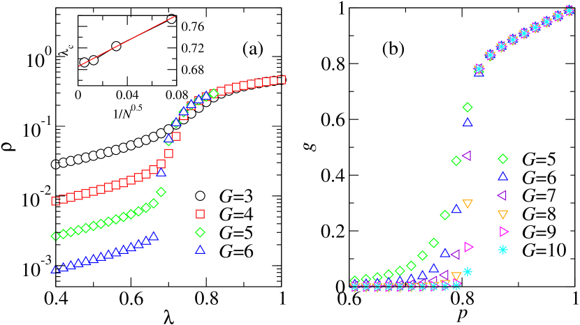
A numerical evidence, however, shows Eq. (3) is not valid. We have performed Monte Carlo simulations for the SIS model on SF networks generated by the $(u,v)$-flower model Rozenfeld07 . It is a deterministic hierarchical model: One starts from two nodes connected with an edge (zeroth generation). Then, every link in a $G$-th generation is replaced with the two $u$- and $v$-link-long paths in the next $(G+1)$-th generation. It results in a SF network with $\gamma=1+\ln(u+v)/\ln 2$ in the $G\rightarrow\infty$ limit Rozenfeld07 . The $(u,v)$-flower model is particularly useful because one can generate an unclustered network easily. If $u>1$ and $v>1$, the degree of all nodes is doubled and the distance between them becomes farther after each iteration. We used the $(3,3)$-flower model in simulations which certainly belongs to the unclustered network. The numerical data shown in Fig. 1 (a) strongly suggest a transition at nonzero $\lambda_{\rm c}$. The threshold can be estimated from the peak positions of the susceptibility $\chi\equiv N(\langle\rho^{2}\rangle-\langle\rho\rangle^{2})/\langle\rho\rangle$ where $N$ is the total number of nodes Ferreira12 . The inset in Fig. 1 shows the peak position is extrapolated to $\lambda_{\rm c}\simeq 0.65(5)$ in the infinite system size limit.

Figure 1: (Color online) Density of infected nodes in the $(3,3)$-flowers in (a). The largest cluster density in the DOP (see text) on the same flowers as in (b).

The origin of the inconsistency is an irreversible fluctuation within local active domains due to the stochasticity in microscopic dynamics. Consider a local domain consisting of $V$ nodes where each node is in the infected state with a probability $r$ and the susceptible state with a probability $(1-r$). Then, no matter how rare, there exists a moment when all nodes recover simultaneously by chance. It takes place after a characteristic time $\tau_{V}\sim(1-r)^{-V}\sim e^{rV}$. Once being recovered, the local domain never returns to an active phase unless externally activated. Considering this effect of the irreversible fluctuation, Eq. (3) should be replaced by

$$\rho(t)\simeq\int_{1/\lambda^{2}}^{\infty}dk\ (\lambda k)P(k)e^{-t/\tau_{\lambda k}}\ .$$ (4)

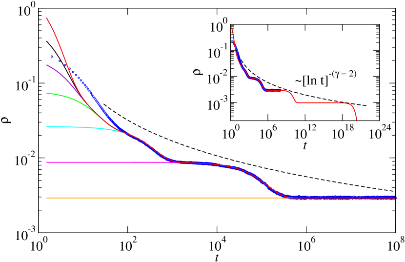
Since it decays to zero eventually, the apparent active phase implied in Eq. (3) is in fact an inactive one. We remark that the inactive phase is different from the usual one in which the density decays exponentially in time. The density in Eq (4) does not decay exponentially fast but extremely slow due to the broad distribution of relaxation times. For example, in SF networks with $P(k)\sim k^{-\gamma}$, one finds

$$\rho(t)\sim[\ln t]^{-(\gamma-2)}~{}.$$ (5)

Equation (4) is numerically tested in the $(3,3)$-flowers at $\lambda=0.56<\lambda_{c}$, which is shown in Fig. 2.

Figure 2: (Color online) $\rho(t)$ in the $(3,3)$-flower of $G=8$. The data points are the SIS model simulation result. The solid curves are obtained from the direct integration of Eq. (4) with two fitting parameters $a_{1}=0.8$ and $a_{2}=0.325$ for $\tau_{\lambda k}=a_{1}e^{a_{2}\lambda k}$ and with the truncated degree distribution function; from bottom to top, $P(k)$ is truncated by $k\geq k_{\rm max}/2^{n}$ with $n=1,2,..,7$. Inset compares the long-time behavior predicted in our theory (red solid curve) with the currently available numerical data (blue dots).

It does not decay exponentially in time. Instead, the density is trapped in a plateau for a while and then decays to another plateau successively. Those plateaus are the evidence for the existence of the metastable local active domains. In the $(u,v)$-flower, degrees of nodes are discretized as $k=2^{n}$ with $n=1,2,..$. So the size $V_{k}\sim\lambda k$ of the local active domains and their life time $\tau_{\lambda k}\sim e^{a\lambda k}$ are also discrete. This discreteness results in the plateaus. As shown, the data in Fig. 2 are fitted to Eq. (4) very well for large $t\gtrsim 10^{2}$. The dashed curve therein represents the overall decay given by Eq. (5).

The slow dynamics given in Eqs. (4) and (5) is reminiscent of a relaxation dynamics in the Griffiths phase Vojta06a ; Hooyberghs03 ; Vojta06 ; Munoz10 . In a disordered system, disorder fluctuations may generate local domains which behave differently from the bulk. Denoting the probability that such a domain of size $\xi$ is realized as $P(\xi)$ and the relaxation time therein as $\tau(\xi)$, a physical quantity $f$ relaxes to its stationary value $f_{s}$ as $\delta f(t)=f(t)-f_{s}\sim\int d\xi P(\xi)e^{-t/\tau(\xi)}$. In the Griffiths phase, the relaxation dynamics is dominated by rare events encoded in the tail of $P(\xi)$ with long characteristic time scales $\tau(\xi)$ Vojta06a . In our case, the slow dynamics is originated from the irreversible fluctuation near hubs.

The previous argument shows that the SIS model on the unclustered network can be in the inactive Griffiths phase for $\lambda_{\rm c}^{\rm QMF}<\lambda<\lambda_{\rm c}$ with a certain nonzero $\lambda_{\rm c}$. It also provides a hint on the mechanism for the phase transition into an active phase. Inside the Griffiths phase, local active domains of size $\sim\lambda k$ are separated [unclustered network] and metastable. As $\lambda$ increases, the size of local domains grow and they begin to overlap each other. The active domains become globally stable when they will form a percolating giant cluster at a certain threshold value of $\lambda$. That is to say, the epidemic transition is triggered by a percolation transition of the local active domains.

Note that the local active domains nucleate around high degree nodes in the degree-descending order. So the uncovered mechanism leads to the conjecture that the unclustered network with $\lambda_{c}\neq 0$ should have a nonzero percolation threshold in the DOP model. Recall that the DOP is suggested as a percolation model where nodes are occupied in the degree-descending order comment . A nonzero percolation threshold $p_{c}$ for the node occupation probability implies that high degree nodes are well separated from each other. Hence, in the context of the SIS model, one requires a nonzero value of $\lambda$ for the local active domains (of size $\sim\lambda k$) to form a percolating cluster.

We provide a numerical evidence of our claim. Figure 1 (b) shows the the percolation order parameter $g$, the density of nodes in the largest cluster, for the DOP in the same $(3,3)$-flowers used in (a). The percolation threshold $p_{\rm c}$ is clearly nonzero, which is consistent with the fact that $\lambda_{c}\neq 0$ as shown in Fig. 1 (a). As another example for the validity of the claim, one may revisit the aforementioned $k_{\rm max}$-star graph case with large $L$. In this example, one can easily find that $p_{\rm c}\neq 0$ supporting our claim.

We also consider the opposite case with $p_{\rm c}=0$. It is achieved only when any finite fraction of occupied nodes in the DOP process are connected to each other to form a percolation cluster. Those networks with $p_{c}=0$ will be called the clustered network. In the context of the SIS model, the local active domains in the clustered network form a percolating cluster even in the limit $\lambda\to 0$. Therefore, we expect that the epidemic threshold is zero in the clustered network. The steady state density of the infected nodes can be expected to scale as

$$\rho\sim\int_{1/\lambda^{2}}^{\infty}dkP(k)\ .$$ (6)

In comparison with Eq. (3), the factor $(\lambda k)$ is missing because a stable active domain consists mainly of high-degree nodes with $k>1/\lambda^{2}$. In scale-free networks with $P(k)\sim k^{-\gamma}$, one obtains $\rho\sim\lambda^{2\gamma-2}$. Note that the order parameter exponent $\beta=2\gamma-2$ is different from $\beta_{\rm QMF}=1$ obtained from the simple QMF theory where only the largest eigenmode was taken into account Mieghem12 .

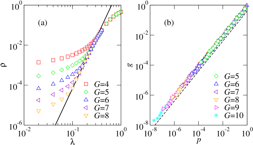
A trivial example of the clustered network is the $k_{\rm max}$-star graph with $L=1$. The density of the largest cluster is given by $g=p$ implying that $p_{c}=0$. Independently, $\lambda_{\rm c}=0$ obviously as discussed in Ref. Castellano10 . A nontrivial example is the $(u,v)$-flowers with $u=1$ (or $v=1$). Recall that if two nodes are connected with an edge in a certain generation, then they remain being connected afterward when $u=1$ (or $v=1$). So one can expect that high degree nodes are clustered. In Fig. 3(a), we present the SIS model simulation results on the $(1,5)$-flowers at several generations $G$. As $G$ increases, the data approach the theoretical prediction $\rho\sim(\lambda-\lambda_{c})^{\beta}$ with $\lambda_{c}=0$ and $\beta=2\gamma-2=2\ln 6/\ln 2$. The DOP property is presented in Fig. 3(b). The scaling of $g\sim p$ therein indicates $p_{c}=0$.

Figure 3: (Color online) Density of infected nodes in the $(1,5)$-flower in (a). The largest cluster density in the DOP on the same flower in (b). The solid lines in (a) has a slope $2\ln 6/\ln 2\simeq 5.19$ while the dashed line in (b) has a slope 1.

What is the epidemic threshold in more interesting cases such as generic random SF networks? Recently, extensive Monte Carlo simulations were performed in random SF networks generated from the configuration model Ferreira12 . However, due to a strong finite-size effect, it still remains inconclusive whether $\lambda_{\rm c}=0$ or not even with simulations of system sizes up to $N=3\times 10^{7}$.

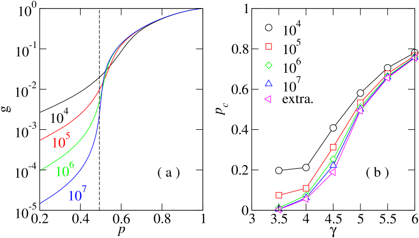
Alternatively we investigate the DOP property of the configuration model networks. In Fig. 4(a) we present the percolation order parameter for the network with $\gamma=5$.

Figure 4: (Color online) (a) The density of the largest DOP cluster in random SF networks of the configuration model with $\gamma=5$. The dashed line denotes the percolation transition point. (b) Maximum cluster heterogeneity points and their extrapolated values. The system sizes are $N=10^{4},..,10^{7}$.

As in the $(3,3)$-flower, the system undergoes the percolation transition at a finite threshold. In order to estimate the percolation threshold precisely, we make use of a so-called cluster heterogeneity (CH) which denotes the number of distinct cluster sizes Lee11 . It was shown Noh11 that $p_{\rm c}(N)$ at which the CH is maximum in networks of size $N$ converges to the percolation threshold $p_{\rm c}$ in the infinite $N$ limit. In Fig. 4(b), we present the numerical data for $p_{\rm c}(N)$ at several values of $\gamma$ and their extrapolated values. The percolation threshold is nonzero unless a small $\gamma$ is considered. Thus, the random SF networks therein belong to the unclustered network class. It provides an indirect evidence that the epidemic threshold could be nonzero on those SF networks.

In summary, we present a theoretical argument that the epidemic threshold of the SIS model on complex networks is nonzero in the unclustered network while it is zero in the clustered network. This conclusion is drawn by taking account of the effect of the irreversible fluctuation which was ignored in the QMF theory. The fluctuation makes a local active domain unstable and leads to the Griffiths phase. Numerical simulations performed in the deterministic $(u,v)$-flowers support our argument. We suggest that the clustering property of a network can be determined by the DOP. By studying the DOP transition, the random SF networks are shown to belong to the unclustered network unless a small degree exponent is considered. It suggests the epidemic threshold in such SF networks is nonzero as opposed to the QMF prediction. Our work raises various interesting questions on the critical phenomenon associated with the epidemic transition and the DOP transition, which are left for future works.

This work was supported by the National Research Foundation of Korea (NRF) grant funded by the Korea government (MEST) (No. 2012-0005003). We thank Prof. Hyunggyu Park for helpful discussions.

References

- (1) A. Barrat, M. Barthélemy, and A. Vespignani, Dynamical Processes on Complex Networks (Cambridge University Press, Cambridge, 2008).
- (2) S.N. Dorogovtsev, A.V. Godtsev, and J.F.F. Mendes, Rev. Mod. Phys. 80, 1275 (2008).
- (3) R. Cohen, S. Havlin, and D. ben-Avraham, Phys. Rev. Lett. 91, 247901 (2003).
- (4) M. Kitsak, L. K. Gallos, S. Havlin, F. Liljeros, L. Muchnik, H. E. Stanley, and H. A. Makse, Nat. Phys. 6, 888 (2010).
- (5) R. Albert and A.-L. Barabási, Rev. Mod. Phys. 74, 47 (2002).
- (6) R. Pastor-Satorras and A. Vespignani, Phys. Rev. Lett. 86, 3200 (2001).
- (7) R. Pastor-Satorras and A. Vespignani, Phys. Rev. E 63, 066117 (2001).
- (8) C. Castellano and R. Pastor-Satorras, Phys. Rev. Lett. 100, 148701 (2008).
- (9) J. D. Noh and H. Park, Phys. Rev. E 79, 056115 (2009).
- (10) S. H. Lee, M. Ha, H. Jeong, J. D. Noh, and H. Park, Phys. Rev. E 80, 051127 (2009).
- (11) C. Castellano and R. Pastor-Satorras, Phys. Rev. Lett. 105, 218701 (2010).
- (12) P. Van Mieghem, Europhys. Lett. 97, 48004 (2012).
- (13) C. Castellano and R. Pastor-Satorras, Sci. Rep. 2, (2012).
- (14) A. V. Goltsev, S. N. Dorogovtsev, J. G. Oliveira, and J. F. F. Mendes, Phys. Rev. Lett. 109, 128702 (2012)
- (15) S. C. Ferreira, C. Castellano, and R. Pastor-Satorras, Phys. Rev. E 86, 041125 (2012).
- (16) J. Hooyberghs, F. Iglói, and C. Vanderzande, Phys. Rev. Lett. 90, 100601 (2003); Phys. Rev. E 69, 066140 (2004).
- (17) T. Vojta, J. Phys. A 39, R143 (2006).
- (18) M. A. Muñoz, R. Juhász, C. Castellano, and G. Ódor, Phys. Rev. Lett. 105, 128701 (2010).
- (19) H. D. Rozenfeld, S. Havlin, and D. ben-Avraham, New J. Phys. 9, 175 (2007).
- (20) Y. Wang et al., 22nd International Symposium on Reliable Distributed Systems (SRDS’03) (IEEE, 2003), p.25.
- (21) D. Stevanović, Linear Algebra Appl. 360, 35 (2003).
- (22) F. Chung, L. Lu, and V. Vu, Proc. Natl. Acad. Sci. U.S.A. 100, 6313 (2003) ;
- (23) R. R. Nadakuditi and M. E. J. Newman, arXiv:1208.1275 (2012).
- (24) T. Vojta, J. Phys. A 36, R143 (2006).
- (25) The DOP is an extreme case of a percolation model with a degree-dependent occupation probability considered in Ref. Gallos05 .
- (26) L. K. Gallos, R. Cohen, P. Argyrakis, A. Bunde, and S. Havlin, Phys. Rev. Lett. 94, 188701 (2005).
- (27) H. K. Lee, B. J. Kim, and H. Park, Phys. Rev. E 84, 020101 (2011).
- (28) J. D. Noh, H. K. Lee, and H. Park, Phys. Rev. E 84, 010101 (2011).