Detection-Directed Sparse Estimation using Bayesian Hypothesis Test and Belief Propagation

Abstract

In this paper, we propose a sparse recovery algorithm called detection-directed (DD) sparse estimation using Bayesian hypothesis test (BHT) and belief propagation (BP). In this framework, we consider the use of sparse-binary sensing matrices which has the tree-like property and the sampled-message approach for the implementation of BP.

The key idea behind the proposed algorithm is that the recovery takes DD-estimation structure consisting of two parts: support detection and signal value estimation. BP and BHT perform the support detection, and an MMSE estimator finds the signal values using the detected support set. The proposed algorithm provides noise-robustness against measurement noise beyond the conventional MAP approach, as well as a solution to remove quantization effect by the sampled-message based BP independently of memory size for the message sampling.

We explain how the proposed algorithm can have the aforementioned characteristics via exemplary discussion. In addition, our experiments validate such superiority of the proposed algorithm, compared to recent algorithms under noisy setup. Interestingly the experimental results show that performance of the proposed algorithm approaches that of the oracle estimator as SNR becomes higher.

I Introduction

Sparse signal recovery in the presence of noise has been intensively investigated in many recent literature because any real-world devices are subject to at least a small amount of noise. We refer to such problems as noisy sparse signal recovery (NSR) problems. Let $\mathbf{x}_{0}\in\mathbb{R}^{N}$ denote a sparse signal vector whose elements are sparsely non-zeros. Then, the NSR decoder observes a measurement vector $\mathbf{z}=\mathbf{\Phi}\mathbf{x}_{0}+\mathbf{n}\in\mathbb{R}^{M}$, where $\mathbf{\Phi}\in\mathbb{R}^{M\times N}$ is a fat sensing matrix $(M\leq N)$; and we limit our discussion to zero-mean independently identically distributed (i.i.d.) Gaussian noise denoted by $\mathbf{n}\in\mathbb{R}^{M}$.

The NSR problem can then be defined as an $l_{0}$-norm minimization problem as similarly done in [1],[3],[7],[8]:

$$\widehat{\bf{x}}_{0,l_{0}}=\arg\mathop{\min}\limits\left\|{\bf{x}}\right\|_{0}\,\,\,\,\,\,s.t.\,\,\left\|{{\bf{\Phi}}\mathbf{x}-{\bf{z}}}\right\|_{2}^{2}\leq\epsilon,$$ (1)

where $\epsilon$ is an error tolerance parameter. In general, the minimization task in (1) is NP hard; therefore, $l_{1}$-norm approaches have been developed and discussed as alternatives [1]-[6]. Among the $l_{1}$-solvers, the Dantzig selector (L1-DS), proposed by Candes and Tao [5], and the $l_{1}$-penalized least-square algorithm usually called LASSO [6] has been devised for the Gaussian noise setup.

Bayesian approaches to NSR have also received attention, where the minimization task in (1) is described as the maximum a posteriori (MAP) problem, and the sparse solution then is sought by imposing sparsifying prior density on $\mathbf{x}$ as follows [8]-[12]:

$$\begin{array}[]{l}\mathbf{\widehat{x}}_{0,\text{MAP}}=\arg\mathop{\max}\limits_{\mathbf{x}}\,\,f_{\mathbf{X}}(\mathbf{x}|\mathbf{Z}=\mathbf{z})\\ \,\,\,\,\,\,\,\,\,\,\,\,\,\,\,\,\,\,\,=\arg\mathop{\max}\limits_{\mathbf{x}}\,\,f_{\mathbf{Z}}(\mathbf{z}|\mathbf{X}=\mathbf{x})f_{\mathbf{X}}(\mathbf{x})\end{array}$$ (4)

where $f(\cdot)$ is a probability density function (PDF).

The task in (4) is likewise computationally demanding; hence, many relaxed-Bayesian solvers have been devised according to various prior types and applied techniques, such as sparse Bayesian-learning (SBL) [9]-[13],[20], Approximate minimum-mean-squared-error (AMMSE) estimation [14]-[17], and belief propagation (BP) with sparse sensing matrices (BP-SM) [18]-[21]. A summary of the relaxed-Bayesian solvers is in Table I.

TABLE I: Relaxd-Bayesian solvers for sparse estimation

Algorithm type	Sensing matrix type	Prior type	Utilized techniques
BP-SM	Sparse-ternary [18],[19]	Gaussian-mixture [18],[19]	Belief-Propagation (BP) [18],[19]
	Sparse-binary [20],[21]	Hierarchical-Gaussian [20],[21]	Expectation-maximization (EM), BP [20],[21]
	Gaussian-random [14]	Spike-and-slab [14]	Fast-Bayesian-Matching-Pursuit [14]
AMMSE	Training-based [15]	Gaussian-mixture [15],[16]	Random-OMP [15]
	Random-unitary [16]		Closed-form-MMSE [16]
	Gaussian-kernel [9]	Hierarchical-Gaussian [9]-[11]	Relevance-vector-machine, EM [9]-[12]
SBL	Gaussian-random [10]-[13]	Spike-and-slab [13]	Markov-chain-Monte-Carlo [13]
	Uniform-random [12]	Hierarchical-Laplace [12]

We are mainly interested in the BP-SM framework, in this paper, which has been investigated as a low-computational approach to solve linear estimation problems such as $\mathbf{z}=\mathbf{\Phi}\mathbf{x}_{0}+\mathbf{n}$. In this framework, the matrix $\mathbf{\Phi}$ is assumed to be a sparse matrix which has the tree-like property, and the statistical connection of $\mathbf{x}_{0}$ and $\mathbf{z}$ is described with the bipartite graph model of $\mathbf{\Phi}$. The tree-like property ensures that the corresponding graph is asymptotically cycle-free [23],[24],[33]. In addition, it is known that the vector finding problem can be decomposed to a sequence of scalar finding problems in the BP-SM framework, where marginal posterior for each scalar estimation is obtained by an iterative message-passing process. This decomposition have been explained by decoupling principle [22],[24].

For implementation of BP, two approaches have been mainly discussed according to the message representation: 1) the sampled-message based BP [27],[28] where the message is directly sampled from the corresponding PDF with a certain step size such that the message is treated as a vector, and 2) the parametric-message based BP (also called relaxed BP) [23],[29],[30] where the message is described as a function with a certain set of parameters such as mean and variance. If the sampled-message approach is chosen, quantization error will be induced according to the step size. If the parametric-message approach is used, some model approximation must be applied for stable iteration at the expense of approximation error.

As applications of the BP-SM approach, the low-density parity-check coding [31]-[33] and the CDMA multiuser detection problems [22],[25],[26] are well known in addition to the NSR works [18]-[21].

Based on the rigorous theoretical support for the BP-SM framework by Guo et al. [22]-[25] and Tanaka et al. [26], and motivated by recent NSR works by Baron et al. [18],[19], Tan et al. [20], and Akcakaya et al. [21], in this paper, we aim to develop a BP-SM type algorithm as an alternative for solving (4). We refer to the proposed algorithm as Detection-directed sparse estimation via Bayesian hypothesis test and belief propagation (BHT-BP). Differently from the works [18]-[21] solving the MAP problem in (4), the proposed algorithm takes a structure of detection-directed (DD) estimation which consists of a signal support detector and a signal value estimator. The support detector is designed using a combination of the sampled-message based BP and a novel Bayesian hypothesis test (BHT), and the signal value estimator behaves in minimum mean-square error (MMSE) sense. The DD-structure considers the common procedure of first using the measurements at hand to detect the signal support set. This detected support is then used in the model of the sparse signal, and an MMSE estimator finds the signal values as if the detected support set is in fact the correct set.

This DD-methodology was originally investigated by Middleton et al. for estimation of noisy signals [36], and includes wide application areas, such as communication systems [37],[38] and speech processing [39]. For NSR, a line of previous works in the AMMSE group has independently studied similar structures by Schnitter et al., Elad et al., and Lee in [14]-[17],[40].

Then, the proposed algorithm achieves the following properties:

1. Providing robust signal support detection against the measurement noise,

2. Removing quantization effect caused by the use of the sampled-message based BP.

Here, the “oracle estimator” implies the estimator which has the perfect support knowledge.

The combination of BHT and BP enables robust detection of the signal support against measurement noise, which was partially introduced in our previous work [43]. In the support detection, the sampled-message based BP provides marginal posterior for each scalar problem according to the decoupling principle, and the BHT-process then detects the supportive state of each scalar element by measuring the inner products between the marginal posterior and reference functions composed of the prior density. This BHT-detector utilizes the signal posterior information more efficiently than the conventional MAP-approaches [18]-[21]. When the measurements are noisy, density spread occurs in marginal posteriors, leading difficulty in making correct decisions via the MAP-approach. In contrast, the BHT-based support detector compensates such a weakpoint by scanning the entire range of the posterior. Such hypothesis-based support detectors have been discussed in wavelet domain denoising problems [41],[42]; however, they were using thresholding techniques to sort out significant wavelet coefficients, different from our work which uses the inner product.

In addition, we emphasize that the proposed algorithm effectively removes quantization effect coming from the use of the sampled-message based BP. The quantization effect limits performance of the MAP-approach in both the signal value estimation and the support detection. In the proposed algorithm, the use of the DD-structure makes the performance independent of the message sampling in the BP. In addition, we eliminate the quantization error in the support detection by applying the minimum value of the signal on its support, denoted by $x_{min}$, to the reference functions. The importance of $x_{min}$ in the NSR problems was theoretically highlighted by Wainwright et al. in [34],[35] where they showed that the perfect support recovery is very difficult even with arbitrarily large SNR if $x_{min}$ is very small. Hence, we regulate $x_{min}$ in our signal model, reflecting the knowledge of $x_{min}$ in the BHT-detection. To the best of our knowledge, we have not seen the reflection of $x_{min}$ in practical algorithms in the sparse recovery literature, and surprisingly, this reflection enables performance of the proposed algorithm to approach that of the oracle estimator as SNR increases.

The computational complexity of the proposed algorithm is $O(N\log N+KM)$ (if the cardinality of the support is fixed to $K$), which includes an additional cost $O(KM)$ owing to the BHT-process to the cost of BP $O(N\log N)$. Nevertheless, the cost of the proposed algorithm is lower in practice since the proposed algorithm can catch the signal support with smaller memory size than NSR algorithms only using the sampled-message based BP.

The remainder of the paper is organized as follows. We first briefly review a line of the BP-SM algorithms, and then make a remark for the relation between the BP-SM solvers and approximate message passing (AMP)-type algorithms in Section II. In Section III, we define our problem formulation. Section IV provides precise description for the proposed algorithm and Section V provides exemplary discussion to explain and support strengths of the proposed algorithm. In Section VI, we provide experimental validation to show the advantage of the proposed algorithm and compare to the recent algorithms. Finally, we conclude the paper in Section VII.

II Related Works

In this section, we provide a brief introduction to the previous works in the BP-SM algorithms [18]-[21]. The common feature in these algorithms is the use of BP in conjunction with sparse sensing matrices, to approximate the signal posterior, where a sparsifying prior is imposed according to the signal model. In addition, we make a remark to distinguish the BP-SM works from AMP-type algorithms.

II-A BP-SM Algorithms

Baron et al. for the first time proposed the use of BP to the sparse recovery problem with sparse sensing matrices [18],[19]. The algorithm is called CS-BP. Signal model of CS-BP is a compressible signal which has a small number of large elements and a large number of near-zero elements. The author associated this signal model with two-state mixture Gaussian prior, given as

$${f_{\mathbf{X}}}(\mathbf{x})=\prod\limits_{i=1}^{N}{q\mathcal{N}(x_{i};0,\sigma_{{X_{1}}}^{2})+(1-q)\mathcal{N}(x_{i};0,\sigma_{{X_{0}}}^{2})},$$ (5)

where $q\in[0,1)$ denotes the probability that an element has the large value, and $\sigma_{X_{1}}\gg\sigma_{X_{0}}$. Therefore, the prior is fully parameterized with $\sigma_{X_{0}},\sigma_{X_{1}}$, and $q$. CS-BP performs MAP or MMSE estimation using the signal posterior obtained from BP, where the authors applied both the sampled-message and the parametric-message approaches for the BP-implementation. The recovery performance is not very good when measurement noise is severe since the CS-BP was basically designed under noiseless setup.

Tan et al. proposed an algorithm under the BP-SM setup called BP-SBL [20]. This work is based on the SBL-framework [9]-[12] which uses two-layer hierarchical-Gaussian prior models given as

$${f_{\mathbf{X}}}({\bf{x}}|a,b)=\prod\limits_{i=1}^{N}{\int_{0}^{\infty}{\mathcal{N}({x}_{i};0,\tau_{i}^{-1})}f_{\Gamma}({\tau_{i}}|a_{i},b_{i})d{\tau_{i}}},$$ (6)

where $f_{\Gamma}({\tau}|a,b)$ is the hyper-prior following Gamma distribution with its parameters $a_{i},b_{i}$. At each iteration, the parameters $a_{i},b_{i}$ of the prior are estimated using expectation maximization (EM). Therefore, the posterior for the signal estimation is iteratively approximated from the prior. The authors applied the BP-SM setup to reduce the computational cost of EM. BP-SBL is an algorithm using parametric-message based BP where every message is approximated to be a Gaussian PDF which can be fully described by its mean and variance. In addition, BP-SBL is input parameter-free, which means this algorithm is adaptive to any signal models and noise level since EM estimates the parameters associated with any given models during the iteration. However, such parameter estimation will not be accurate when noise is severe; therefore, denoising ability of BP-SBL is limited when measurements are highly corrupted.

Most recently, Akcakaya et al. proposed SuPrEM under a framework similar to BP-SBL which uses a combination of EM and the parametric-message based BP [21]. The main difference from BP-SBL is the use of a specific type of hyper-prior called Jeffreys’ prior $f_{\mathcal{J}}(\tau_{i})=1/\tau_{i}\,\,\forall\tau\in[T_{i},\infty]$. The use of Jeffreys’ prior reduces the number of input parameters while sparsifying the signal. Therefore, the prior is given as

$${f_{\mathbf{X}}}({\bf{x}})=\prod\limits_{i=1}^{N}{\int_{0}^{\infty}{\mathcal{N}({x}_{i};0,\tau_{i})}f_{\mathcal{J}}({\tau_{i}})d{\tau_{i}}}.$$ (7)

The sensing matrix used in SuPrEM is restricted to a sparse-binary matrix which has fixed column and row weights, called low-density frames. They are reminiscent of the regular LDPC codes [31]. In addition, the signal model is confined to $K$-sparse signals consisting of $K$ nonzeros and $N-K$ zeros since SuPrEM includes a spasifying step which choose the $K$ largest elements at each end of iteration. The noise statistic is an optional input to the algorithm. Naturally, if the noise information is available, SuPrEM will provide an improved recovery performance.

Figure 1: Experimental success rate of sparse recovery via the standard AMP under the use of sparse-Gaussian matrices. The success rate is plotted as a function of the matrix sparsity defined as percentage of nonzero entries in the sensing matrix. We record a success if the MSE, defined in (23), is below $10^{-3}$. Reconstruction signal length is $N=1024$ and 500 iterations were used.

II-B Relation to AMPs

It is interesting to associate the algorithms in the BP-SM group to the class of AMP algorithms, which was originally invented by Donoho et al. in [44],[45], analyzed and refined by Bayati et al. [46] and Rangan [47], because both types of the algorithms utilize BP. Performance of the AMPs coincides with that of the $l_{1}$-solvers under the large limit assumption ($N\rightarrow\infty$) in the noiseless case [44],[46]. Furthermore, in a recent result by Donoho et al. showed that performance of the AMPs is also equivalent to LASSO [6] under the noisy setting with appropriate parameter calibration [48].

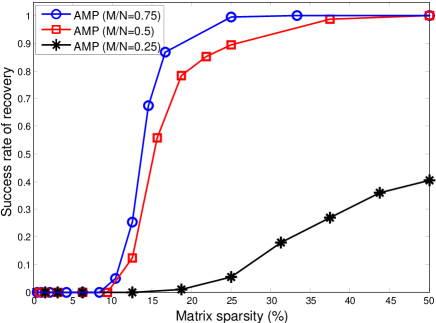
The AMPs work well when sufficient density of the sensing matrix is maintained as $N\rightarrow\infty$ since the AMPs were developed on the basis of an approximation of BP-messages by the central limit theorem [45]. Therefore, if a sparse matrix is applied to the AMPs, the message approximation does not work, then the decoder will fail in the recovery. We validate this claim by our own experimental result shown in Fig.1, where we simulated the recovery success rate of the standard AMP [44] without additive noise as a function of the matrix sparsity defined as percentage of nonzero entries in the sensing matrix. The recovery of the AMP are not successful when the sensing matrix is sparse ( typically less than 10$\%$ matrix sparsity) regardless of the number of measurements $M$, as shown in an example of Fig.1. Namely, the AMPs recover sparse signals well with dense matrices at the expense of low computation $O(MN\log N)$, but it does not enjoy the benefits from the use of sparse matrices.

III Problem Formulation

The goal of the proposed algorithm is to recover the object signal $\widehat{\mathbf{x}}_{0}$ given the knowledge of $\mathbf{\Phi}$ and noisy measurements $\mathbf{z}$ as following

$$\mathbf{z}=\mathbf{\Phi}\mathbf{x}_{0}+\mathbf{n},$$ (8)

where we consider the use of a fat sparse-binary sensing matrix $\mathbf{\Phi}\in\{0,1\}^{M\times N}$ $(M<N)$ which has very low matrix sparsity (typically less than 10$\%$ matrix sparsity) and the tree-like property. We regulate the matrix sparsity using the fixed column weight $L$ since this regulation enables the matrix $\mathbf{\Phi}$ to span the measurement space with basis having equal energy. For the noise distribution, we assume i.i.d. zero-mean Gaussian density such that the noise vector $\mathbf{n}\in\mathbb{R}^{M}$ is drawn from ${\mathcal{N}(0,\sigma_{N}^{2}\mathbf{I})}$.

In the remainder of this section, we introduce some necessary concepts, such as signal model and graph representation of $\mathbf{\Phi}$, for our framework, and then discuss our approach to solve this NSR problem.

III-A Graph Representation of $\mathbf{\Phi}$

Bipartite graphs effectively represent linear systems with sparse matrices such as the matrix $\mathbf{\Phi}$. Let $\mathcal{V}:=\{1,...,N\}$ denote the set of indices corresponding to the elements of the signal vector, $\mathbf{x}_{0}=[x_{0,1},...,x_{0,N}]$, and $\mathcal{C}:=\{1,...,M\}$ denote the set of indices corresponding to the elements of the measurement vector, $\mathbf{z}=[z_{1},...,z_{M}]$. In addition, we define the set of edges connecting $\mathcal{V}$ and $\mathcal{C}$ as $\mathcal{E}:=\{(j,i)\in\mathcal{V}\times\mathcal{C}\,|\,\,\phi_{ji}=1\}$ where $\phi_{ji}$ is the $(j,i)$-th element of $\mathbf{\Phi}$. Then, a bipartite graph $\mathcal{G}=(\mathcal{V,C,E})$ fully describes the neighboring relation in the linear system. For convenience, we define the neighbor set of $\mathcal{V}$ and $\mathcal{C}$ as $N_{\mathcal{V}}(i):=\{j\in\mathcal{C}\,|(j,i)\in{\mathcal{E}}\}$ and $N_{\mathcal{C}}(j):=\{i\in\mathcal{V}\,|(j,i)\in{\mathcal{E}}\}$, respectively. Note that $\left|N_{\mathcal{V}}(i)\right|=L$ under our setup on $\mathbf{\Phi}$.

Figure 2: DD-estimation in the proposed algorithm

III-B Signal Model

Let $\mathbf{x}_{0}\in\mathbb{R}^{N}$ denote a sparse vector which is a deterministic realization of a random vector $\mathbf{X}$. Here, we assume that the elements of $\mathbf{X}$ are i.i.d., and each $X_{i}$ belongs to the support set, denoted by $supp(\mathbf{X})$, with a rate $q\in[0,1]$. To indicate the supportive state of $X_{i}$, we define a state vector $\mathbf{S}(\mathbf{X})$ where each $S_{i}\in\mathbf{S}(\mathbf{X})$ is defined as

$${S_{i}}=S(X_{i})=\left\{\begin{array}[]{l}1,\,\,\,\,\,{\rm{if}}\,\,i\in supp(\mathbf{X})\\ 0,\,\,\,\,\,{\rm{else}}\end{array}\right.\text{ for all }\,\,i\in\mathcal{V}.$$ (11)

Therfore, the signal sparsity is given as $K=||\mathbf{S}||_{0}$. For the signal values on the support, we will deal with two cases, which are

1. Gaussian signals:$\,X_{i\in supp(\mathbf{X})}\sim\mathcal{N}(0,\sigma_{X_{1}}^{2})$,

2. Signed signals :$\,\,\,\,\,X_{i\in supp(\mathbf{X})}\sim\frac{1}{2}\delta_{-\sigma_{X_{1}}}+\frac{1}{2}\delta_{+\sigma_{X_{1}}}$,

where $\delta_{\tau}$ denote the delta function peaked at $\tau$. Namely, in the first case, the values on the support are distributed according to an i.i.d. zero-mean Gaussian density with variance $\sigma_{X_{1}}^{2}$, and in the second case the magnitude of the values is fixed to $\sigma_{X_{1}}$ and the sign follows Bernoulli distribution with probability $1/2$. In addition, for the Gaussian signal, we regulate the minimum value $x_{min}$ on the support as a key parameter of the signal model, such that

$$x_{min}\leq|x_{0,i}|\,\,\,\text{ for all }i\in supp(\mathbf{x}_{0}),$$ (12)

Indeed, Wainwright et al. emphasized the importance of $x_{min}$ in the NSR problems [34],[35]. They stated that if $x_{min}$ is very small, success of the noisy sparse recovery is very difficult even with arbitrarily large SNR. Namely, if the signal contains at least such a very small element belonging to the support, the recovery can be failed regardless of SNR level since the small element can be buried even by negligible noise.

In the Bayesian framework, the prior density takes a role of pursuing the sparsest solution from infinitely many solutions of the underdetermined system. Therefore, the proper choice of the sparsifying prior according to the signal model is highly important. According to our signal model, we consider spike-and-slab densities as our prior. The prior for an element $X_{i}$ is given as

$$\begin{array}[]{l}f_{X}(x)=qf_{X}(x|S=1)+(1-q)f_{X}(x|S=0)\\ \,\,\,\,\,\,\,\,\,\,\,\,\,\,\,\,\,\,\,=q\mathcal{N}(x;0,\sigma_{X_{1}}^{2})+(1-q)\delta_{0}.\end{array}$$ (15)

This type of the priors has been widely used in modeling of strictly sparse signals [13],[14],[53] since the prior can simply characterize the signals with $\sigma_{X_{1}}$ and $q$, as well as easily associate the signal model with the other models such as hidden Markov chain and wavelet model. In addition, we note that the spike-and-slab prior is a particular case of two-state Gaussian mixture in (5) as $\sigma_{X_{0}}\rightarrow 0$.

III-C Solution Approach

The approach of the DD-estimation is motivated by the naive MMSE sparse estimation which was also reported in [14]-[16], as follows:

$${\widehat{\bf{x}}_{0,\text{MMSE}}}=\sum\limits_{{\bf{s}}\in{{\{0,1\}}^{N}}}{{\bf{E}}[{{\bf{X}}}|{\bf{S}},{\bf{Z}}={\bf{z}}]\cdot\Pr\{{\bf{S}}|{\bf{Z}}={\bf{z}}\}\,},$$ (16)

We note that (16) is a weighted sum of the signal value estimation ${\bf{E}}[{{\bf{X}}}|{\bf{S}},{\bf{Z}}={\bf{z}}]$ over $2^{N}$ possible supports given noisy measurements $\mathbf{z}$. Therefore, we separate the signal value estimation and the $2^{N}$ support searching in (16) as the first step for its relaxation. Then, the signal value estimation can be represented as

$${\widehat{\bf{x}}_{0,\text{BHT-BP}}}={\bf{E}}\left[{{{\bf{X}}}|{\bf{S}}={\widehat{\bf{s}}},{\bf{Z}}={\bf{z}}}\right],$$ (17)

by assuming an ideal support detector for $\widehat{\bf{s}}$. The calculation of (17) is simple because it is well known as the convectional linear MMSE estimation, expressed as

$${\widehat{\bf{x}}_{0,\widehat{\bf{s}}}}={\left({\frac{1}{{\sigma_{X_{1}}^{2}}}{\bf{I}}+\frac{1}{{\sigma_{N}^{2}}}{\bf{\Phi}}_{\widehat{\bf{s}}}^{T}{\bf{\Phi}}_{\widehat{\bf{s}}}}\right)^{-1}}\frac{1}{{\sigma_{N}^{2}}}{\bf{\Phi}}_{\widehat{\bf{s}}}^{T}{\bf{z}},$$ (18)

where $\mathbf{\Phi}_{\widehat{\mathbf{s}}}\in\{0,1\}^{M\times K}$ as a submatrix of $\mathbf{\Phi}$ that contains only the columns corresponding to the detected support $\widehat{\mathbf{s}}$, and $\mathbf{x}_{0,\widehat{\mathbf{s}}}\in\mathbb{R}^{K}$ as a vector that includes only the nonzero elements from $\widehat{\bf{x}}_{0}$. In addition, we know that this MMSE estimation is optimal when the signal values on the detected support $\widehat{\bf{s}}$ are Gaussian distributed [49].

For the part of the $2^{N}$ support search, we start from an exhaustive detection, described as

$$\widehat{\bf{s}}=\arg\mathop{\max}\limits_{\mathbf{s}\in\{0,1\}^{N}}\Pr\{{\bf{S}}={\bf{s}}|{\bf{Z}}={\bf{z}}\}.$$ (19)

To solve (19) efficiently, we decompose the state vector detection to $N$ scalar state detections based on the decoupling principle [22],[24], and apply binary scalar MAP-detection for each scalar state. Then, the binary scalar detection can be optimally achieved by a hypothesis test [50], given as

$${\frac{{\Pr\{S_{i}=1|{\bf{Z}}={\bf{z}}\}}}{{\Pr\{S_{i}=0|{\bf{Z}}={\bf{z}}\}}}}\mathop{\mathop{\gtrless}\limits_{{H_{0}}}}\limits^{{H_{1}}}1\text{ for all }i\in\mathcal{V},$$ (20)

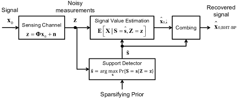
where $H_{0}:S(X_{i})=0$ and $H_{1}:S(X_{i})=1$ are two possible hypotheses. This support detection approach simplifies the $2^{N}$ exhaustive search in (19) to $N$ hypothesis tests. Here, we note that the support detection in (20) performs with an independent decision rule from the value estimation in (18). Therefore, this DD-approach to (16) is reasonable since the Bayesian risks of the support detection and the signal values estimation can be independently minimized [36]. The overall flow of the DD-estimation is depicted in Fig.2.

In order to justify our solution approach, we will provide experimental validation compared to the recent NSR algorithms, as a function of SNR defined as

$$\text{SNR }:=10\log_{10}\frac{{E{\left\|{{\bf{\Phi}}\mathbf{x}_{0}}\right\|_{2}^{2}}}}{{M\sigma_{N}^{2}}}\text{ dB }.$$ (21)

Performance of the support detection is evaluated pairwise state error rate (SER), defined as

$${\text{SER}}:=\Pr\{s(x_{0,i})\neq\widehat{s}_{i}|i\in\mathcal{V}\},$$ (22)

and the overall performance of the signal recovery is measured in terms of normalized mean square error (MSE), defined as

$${\text{MSE}}:=\frac{{\left\|{\widehat{\bf{x}}_{0}-{\bf{x}}_{0}}\right\|_{2}^{2}}}{{\left\|{\bf{x}}_{0,\mathbf{s}}\right\|_{2}^{2}}}.$$ (23)

IV Proposed Algorithm

The proposed algorithm straightforwardly provides the estimate $\widehat{\mathbf{x}}_{0}$ via the MMSE estimation in (18) once given the detected support set $\widehat{\mathbf{s}}$ from (19). In addition, we state that the detected support set can be elementwisely obtained from (20), on the basis of the decoupling principle. Therefore, efficient design of the scalar state detector in (20) is very important in this work. In this section, we explain the implementation of the scalar state detector based on the hypotesis test given in (20), using the combination of the sampled-message based BP and BHT.

Figure 3: Graph representation of the sampled-message based BP ($N=6,M=4,L=2$), where $\otimes$ is the operator for the linear convolution of PDFs and $\delta_{z_{j}}$ indicates the delta function peaked at $z_{j}$.

IV-A Sampled-message based Belief Propagation

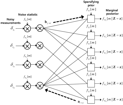
BP provides the marginal posterior for the hypothesis test in (20) for each element. Since the signal is real-valued, each BP-message takes the form of a PDF, and the BP-iteration consists of density-message passing. We provide a brief summary of density-message passing in Appendix I. To implement the BP passing density-messages, we consider the sampled-message approach which has been discussed by Sudderth et al. [27], and Noorshams et al. [28]. For the sparse recovery, Baron et al. applied the approach in [18],[19]. The main strength of the sampled-message approach is adaptivity to various signal models. In addition, it shows faster convergence than the parametric-message approach [23],[29],[30] if the sampling step size is sufficiently fine. The reason is that the sampled-message approach does not use any model approximation or reduction for the message representation during the iteration. Based on (50) and (Appendix I Fundamentals of Density-message Passing) from Appendix I, we will provide a practical message update rule of the sampled-message based BP for the proposed algorithm.

In our implementation, we set the sampling step $T_{s}$ on the basis of the three sigma-rule [52], given as

$$T_{s}=\frac{2\cdot 3\sigma_{X_{1}}}{N_{d}}$$ (24)

where $N_{d}$ is the number of samples for a density-message. Hence, we define the sampling process of the PDFs as

$$\begin{array}[]{l}{\rm{Samp}}\left[{f(x)}\right]:=f(m{T_{s}}-3{\sigma_{X_{1}}})\\ \,\,\,\,\,\,\,\,\,\,\,\,\,\,\,\,\,\,\,\,\,\,\,\,\,\,\,\,\,\,\,\,\,\,=f[m]\,\,\,{\rm{for}}\,\,\,m=0\sim{N_{d}}-1,\end{array}$$ (27)

where $\rm{Samp}[\cdot]$ denotes the sampling process. Hence, the density-messages are treated as vectors with size $N_{d}$ in this approach.

Let $\mathbf{a}_{i\rightarrow j}[m]\in[0,1]^{N_{d}}$ denote a sampled density-message from $X_{i}$ to $Z_{j}$, called the signal message;, and $\mathbf{b}_{j\rightarrow i}[m]\in[0,1]^{N_{d}}$ is the message from $Z_{j}$ to $X_{i}$, called the measurement message. The signal message $\mathbf{a}_{i\rightarrow j}[m]$ includes information on the marginal posterior $f_{X_{i}}(x|\mathbf{Z}=\mathbf{z})$, being obtained from (50) by simply replacing the measurement densities, $f_{Z_{k}}(z|X_{i}=x_{i})$, with the measurement messages of the previous iteration except the intrinsic information. That is,

$$\mathbf{a}_{i\rightarrow j}^{l}[m]=\eta\left[{{f_{X}}[m]\times\prod\limits_{k\in N_{\mathcal{V}}(i)\backslash\{j\}}{{\bf{b}}_{k\rightarrow i}^{l-1}}[m]}\right],$$ (28)

$\text{ for all }(i,j)\in\mathcal{E}$, where $\eta[\cdot]$ is the normalization function to make $\sum{\mathbf{a}_{i\rightarrow j}[m]}=1$. Similarly, the measurement message $\mathbf{b}_{j\rightarrow i}[m]$ includes information on the measurement density $f_{Z_{j}}(z|X_{i}=x_{i})$, being obtained from the expression of (Appendix I Fundamentals of Density-message Passing) by replacing the associated marginal posteriors, $f_{X_{k}}(x|\mathbf{Z}=\mathbf{z})$, with the signal messages, that is,

$$\begin{array}[]{l}\mathbf{b}_{j\rightarrow i}^{l}[m]\\ =\underbrace{{f_{\mathcal{N}}}[m;{z_{j}},\sigma_{N}^{2}]}_{={\rm{Samp}}[\mathcal{N}(n;z_{j},\sigma_{N}^{2})]}\otimes\left(\bigotimes\limits_{k\in N_{\mathcal{C}}(j)\backslash\{i\}}{\mathbf{a}_{k\rightarrow j}^{l}[-m]}\right),\end{array}$$ (31)

where $\otimes$ is the operator for the linear convolution of PDFs. In addition, under the Gaussian noise assumption, we know $\delta_{z_{j}}\otimes f_{N_{j}}(n)=\mathcal{N}(n;z_{j},\sigma_{N}^{2})$ in (31) based on (Appendix I Fundamentals of Density-message Passing). Here, we note that the measurement message calculation utilizes the noise statistics distinctively from that of the standard CS-BP [see (7) in [19]]. This improvement remarkably enhances the recovery performance in the low SNR regime even though the noise statistic loses its effect with sufficiently high SNR.

The convolution operations in (31) can be efficiently computed by using the Fast fourier transform (FFT). Accordingly, we express for the measurement message calculation as

$$\begin{array}[]{l}{\bf{b}}_{j\to i}^{l}[m]\\ =\mathcal{F}^{-1}\left[\mathcal{F}\left[{f_{\mathcal{N}}}[m;{z_{j}},\sigma_{N}^{2}]\right]\left(\prod\limits_{k}{\mathcal{F}[\mathbf{a}_{k\rightarrow j}^{l}[-m]]}\right)\right]\end{array}$$ (34)

where $\mathcal{F}[\cdot]$ denotes the FFT operation. Therefore, for efficient use of FFT, the sampling step $T_{s}$ should be appropriately chosen such that $N_{d}$ is two’s power. In fact, the use of the FFT brings a small calculation gap since the FFT-based calculation performs a circular convolution that produces output having a heavy tail. The heaviness increases as the column weights of $\mathbf{\Phi}$ increases. However, the difference is can be ignored, especially when the messages are bell-shaped densities.

Figure 4: Bayesian hypothesis test for support detection where $r_{0}(x):=\frac{{f_{X}(x|S=0)}}{{f_{X}(x)}},r_{1}(x):=\frac{{f_{X}(x|S=1)}}{{f_{X}(x)}}$ are reference functions consisting of the prior knowledge.

Finally, an sampled approximation of the marginal posterior ${f_{{X_{i}}}}[m|\mathbf{Z}={\bf{z}}]\text{ for }\,\,m=0\sim N_{d}-1$ is obtained after a certain number of iteration $l^{*}$ via the update rule in (28),(31), as follows:

$$\begin{array}[]{l}\text{Samp}[f_{X_{i}}(x|\mathbf{Z}=\mathbf{z})]\approx f_{X_{i}}[m|\mathbf{Z}=\mathbf{z}]\\ \,\,\,\,\,\,\,\,\,\,\,\,\,\,\,\,\,\,\,\,\,\,\,\,\,\,\,\,\,\,\,\,\,\,\,\,\,\,\,\,\,\,\,\,\,\,\,\,\,\,\,\,=\eta\left[{f_{X}[m]\times\prod\limits_{j\in N_{\mathcal{V}}(i)}{{\mathbf{b}_{j\rightarrow i}^{l^{*}}[m]}}}\right].\end{array}$$ (37)

IV-B Bayesian Hypothesis Test for Support Detection

In order to perform the hypothesis test in (20), the decoder needs to calculate the probability ratio $\frac{{\Pr\{S_{i}=0|{\bf{Z}}\}}}{{\Pr\{S_{i}=1|{\bf{Z}}\}}}$. By factorizing over $X_{i}$, the hypothesis test becomes

$${\frac{{\Pr\{S_{i}=1|{\mathbf{Z}=\bf{z}}\}}}{{\Pr\{S_{i}=0|\mathbf{Z}={\bf{z}}\}}}}$$

$$={\frac{{\int{\Pr\{S_{i}=1|{\bf{Z}}=\mathbf{z},X_{i}\}f_{X_{i}}(x|\mathbf{Z}=\mathbf{z})}dx}}{{\int{\Pr\{S_{i}=0|{\bf{Z}}=\mathbf{z},X_{i}\}f_{X_{i}}(x|\mathbf{Z}=\mathbf{z})}dx}}}\mathop{\mathop{\gtrless}\limits_{{H_{0}}}}\limits^{{H_{1}}}1.$$ (38)

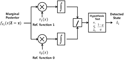
In practice, we replace the marginal posterior $f_{X_{i}}(x|\mathbf{Z}=\mathbf{z})$ with the sampled marginal posterior $f_{X_{i}}[m|\mathbf{Z}=\mathbf{z}]$ from (37) for discrete signal processing, which is provided in Algorithm 1. However, we use notations of the continuous domain in the description of this hypothesis process. Given $X_{i}=x_{i}$ from BP, the given measurements $\mathbf{z}$ do not provide any additional information on $S_{i}$; hence, $\Pr\{S_{i}|\mathbf{Z}={\bf{z}},X_{i}\}=\Pr\{S_{i}|X_{i}\}$ holds true. Using such a fact and the Bayesian rule, the test in (IV-B) is rewritten as

$${\frac{{\int{r_{1}(x)f_{X_{i}}(x|\mathbf{Z}=\mathbf{z})}dx}}{{\int{r_{0}(x)f_{X_{i}}(x|\mathbf{Z}=\mathbf{z})}dx}}}\mathop{\mathop{\gtrless}\limits_{{H_{0}}}}\limits^{{H_{1}}}{\frac{{\Pr\{S=0\}}}{{\Pr\{S=1\}}}},$$ (39)

where $\frac{\Pr\{S=0\}}{\Pr\{S=1\}}={\frac{(q-1)}{q}}$, and $r_{0}(x),r_{1}(x)$ are reference functions consisting of the prior knowledge defined as

$$r_{0}(x):=\frac{{f_{X}(x|S=0)}}{{f_{X}(x)}},\,\,\,r_{1}(x):=\frac{{f_{X}(x|S=1)}}{{f_{X}(x)}}.$$ (40)

The process to calculate the probability ratio in (39) is described as a block diagram in Fig.4. This process has a similar structure to matched filtering in communication systems, where the detector determines supportive state of $X_{i}$ by measuring inner products between the marginal posterior and reference functions. In addition, we emphasize that this BHT-based detector is only compatible with the sampled-message based BP because the BHT-process requires full information on the signal posterior which cannot be provided through the parametric-message based BP.

Algorithm 1 BHT-BP

Noisy measurements $\mathbf{z}$, Sensing matrix $\mathbf{\Phi}$, Sparsfying prior $f_{X}(x)$, Noise statistic $f_{N}(n)$, Sampling step $T_{s}$, Number of the BP-iterations $l^{*}$.

Reconstructed signal $\widehat{\mathbf{x}}_{0,\text{BHT-BP}}$, Detected state vector $\widehat{\mathbf{s}}$.

1) Sampled-message based BP:

set $\mathbf{b}_{j\rightarrow i}^{l=0}=\mathbf{1}\text{ for all }(i,j)\in\mathcal{E}$

for $l=1$ to $l^{*}$ do

     for $i=1$ to $N$ do

         set $\mathbf{a}_{i\rightarrow j}^{l}[m]=\eta\left[{{f_{X}}[m]\times\prod\limits_{k\in N_{\mathcal{V}}(i)\backslash\{j\}}{{\bf{b}}_{k\rightarrow i}^{l-1}}[m]}\right]$

     end for

     for $j=1$ to $M$ do

         $\begin{array}[]{l}\text{set }\mathbf{b}_{j\rightarrow i}^{l}[m]\\ =f_{\mathcal{N}}[m;{z_{j}},\sigma_{N}^{2}]\otimes\left(\bigotimes\limits_{k\in N_{\mathcal{C}}(j)\backslash\{i\}}{\mathbf{a}_{k\rightarrow j}^{l}[-m]}\right)\end{array}$

     end for

end for

for $i=1$ to $N$ do

     set $f_{X_{i}}[m|\mathbf{Z}=\mathbf{z}]=\eta\left[{f_{X}[m]\times\prod\limits_{j\in N_{\mathcal{V}}(i)}{{\mathbf{b}_{j\rightarrow i}^{l^{*}}[m]}}}\right]$

end for

2) BHT for Support Detection:

set $\gamma=q/(1-q)$

for $i=1$ to $N$ do

     if ${\frac{{\sum_{m}{r_{1}[m]f_{X_{i}}[m|\mathbf{Z}=\mathbf{z}]}}}{{\sum_{m}{r_{0}[m]f_{X_{i}}[m|\mathbf{Z}=\mathbf{z}]}}}}>\frac{(1-q)}{q}$ then set $\widehat{s}_{i}=1$

     else set $\widehat{s}_{i}=0$

     end if

end for

3) Signal Value Estimation:

set ${\widehat{\bf{x}}_{0,\text{BHT-BP}}}={\bf{E}}\left[{{{\bf{X}}}|{\bf{S}}=\widehat{{\bf{s}}},\mathbf{Z}={\bf{z}}}\right]$

IV-C Computational Complexity

In the sampled-message approach, the density-messages in BP are vectors with size $N_{d}$. Therefore, the decoder requires $O(LN_{d})$ flops to calculate a signal message $\mathbf{a}_{i\rightarrow j}$ and $O({\frac{{NLN_{d}}}{M}\log N_{d}})$ flops for a measurement message $\mathbf{b}_{j\rightarrow i}$ per iteration, where $L$ denotes the column weight of the sparse sensing matrix $\mathbf{\Phi}$. In addition, the cost of the FFT-based convolution is $O(N_{d}\log N_{d})$ if we assume the row weight is $NL/M$ using average sense. Hence, the per-iteration cost of the BP-process is $O(NLN_{d}+M{\frac{{NLN_{d}}}{M}\log N_{d}})\approx O(NLN_{d}\log N_{d})$ flops. For the hypothesis test, the decoder requires $O(N_{d})$ flops to generate the probability ratio. The cost for the hypothesis test is much smaller than that of BP; therefore, it is ignored. For the MMSE estimator to find signal values, the cost can be reduced upto $O(KM)$ flops by applying QR decomposition [51]. Thus, the total complexity of the proposed algorithm is $O\left(l^{*}\times NLN_{d}\log N_{d}+KM\right)$ flops and it is further simplified to $O(l^{*}\times N+KM)$ since $L$ and $N_{d}$ are fixed. In addition, it is known that the recovery convergence via BP is achieved with $O(\log N)$ iterations [19],[32]. Therefore, we finally obtain $O(N\log N+KM)$ for the complexity of BHT-BP. We note here that the complexity of BHT-BP is much relaxed from that of the naive MMSE sparse estimator $O(2^{N})$, given in (16).

V Exemplary Discussion for Proposed Algorithm

One can argue the DD-structure of the proposed algorithm is an abuse since the marginal posteriors from the BP already provides full information on the signal. Namely, this means that $f_{X_{i}}[m|\mathbf{Z}=\mathbf{z}]$ in (37) contains the perfect knowledge for detection and estimation of $x_{0,i}$. Yes it is true, but our claim is that the MAP-based algorithms [18],[19] which solve the problem in (4) are not utilizing the full knowledge of the marginal posterior.

In this section, we show two weakpoints of the MAP-approach which finds each scalar estimate $\widehat{x}_{0,i}$ only using the peak location of the marginal posterior, through examples. We then discuss how the proposed algorithm can remedy such problematic behavior of the MAP, and utilize the posterior knowledge more efficiently. We claim that the proposed algorithm has strength in two aspects as given below:

1. Robust support detection against additive noise: The BHT-detector in the proposed algorithm correctly catches the supportive state given $i\in supp(\mathbf{x}_{0})$ even under severe additive noise.

2. Removing quantization effect caused by the sampled-message based BP: The quantization effect degrades performance of the MAP-based algorithms in both the signal value estimation and the support detection. In the proposed algorithm, the DD-structure removes the quantization effect from the signal value estimation, and the BHT-detector reduces the chance of misdetection of the supportive state given $i\notin supp(\mathbf{x}_{0})$ by applying the knowledge of $x_{min}$ to the reference functions.

Figure 5: Example of a marginal posterior $f_{X_{i}}(x|\mathbf{Z}=\mathbf{z})$ in BP-iteration under severe noise (SNR=10 dB), where $x_{0,i}$ originally has nonzero ($x_{0,i}=6.7)$, the minimum value is $x_{min}=1.25$.

Figure 6: Example of a marginal posterior $f_{X_{i}}(x|\mathbf{Z}=\mathbf{z})$ over SNR where $x_{0,i}$ originally has nonzero ($x_{0,i}=6.7)$, the minimum value is $x_{min}=1.25$, and we use 5 BP-iterations to approximate $f_{X_{i}}(x|\mathbf{Z}=\mathbf{z})$.

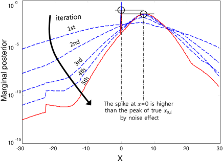
V-A Robust Support Detection against Additive Noise

The additive noise spreads probability mass in the marginal posterior $f_{X_{i}}(x|\mathbf{Z}=\mathbf{z})$, leading to difficulty in the supportive state detection via the MAP-approach given $i\in supp(\mathbf{x}_{0})$. For example, Fig.6 shows marginal posterior obtained from severe noisy measurements (SNR=10 dB) via BP-iteration, where the signal value is originally $x_{i,0}=6.7$, hence $i\in supp(\mathbf{x}_{0})$. We note that the posterior is approximately composed of a zero-spike and a slab-density with certain probability weights. In Fig.6, it is shown that the center of the slab-density is moving to the true value $x=6.7$ over the iterations, but after 5 iterations the mass at $x=6.7$, i.e., $f_{X_{i}}(x=6.7|\mathbf{Z}=\mathbf{z})$, is still smaller than that of the zero-spike. The reason is that the noise effect spreads the slab-density over near values, making the peak at $x=6.7$ to be blunt. We call this spreading effect as density spread.

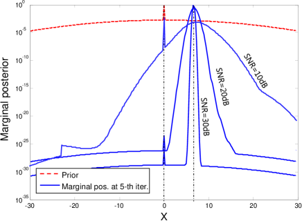
Fig.6 more clearly describes the density spread in the marginal posterior according different SNR levels. When SNR level is sufficiently high (see cases more than SNR=20 dB in Fig.6), the MAP-approach can successfully detect the supportive state since probability mass is concentrated on the center of the slab-density such that $f_{X_{i}}(x=6.7|\mathbf{Z}=\mathbf{z})\geq f_{X_{i}}(x=0|\mathbf{Z}=\mathbf{z})$. However, when SNR is low (see the line of SNR=10 dB in Fig.6), the MAP-approach will fail in the detection because the zero-spike $f_{X_{i}}(x=0|\mathbf{Z}=\mathbf{z})$ becomes the highest peak in the marginal posterior such that $f_{X_{i}}(x=6.7|\mathbf{Z}=\mathbf{z})<f_{X_{i}}(x=0|\mathbf{Z}=\mathbf{z})$ due to the density spread. The density spread does not cause errors given $i\notin supp(\mathbf{x}_{0})$ since in this case the center of the slab-density stays at $x=0$ during the BP-iteration, regardless of the noise level.

In contrast, the BHT-detector in the proposed algorithm, decides the supportive state by considering the density spread effect. In (39), the inner products between $r_{1}(x),r_{0}(x)$ and $f_{X_{i}}(x|\mathbf{Z}=\mathbf{z})$ measure portions of the marginal posterior corresponding to $i\in supp(\mathbf{x}_{0})$ and $i\notin supp(\mathbf{x}_{0})$ respectively. Since the inner products are associated with the entire range of the $x$-axis rather than specific point-mass, the BHT-detector can decide the supportive state by incorporating all spread mass due to noise. Therefore, the BHT-detector can success in the detection even in the SNR=10 dB case of Fig.6. This example supports that BHT-detector has ability to detect the signal support more robustly against noise than the MAP-approach.

Figure 7: Example of measurement message passing under quantization caused by the sampled-message based BP where $T_{s}=0.25$

V-B Removing Quantization Effect caused by the Sampled-message Based BP

V-B1 In signal value estimation

Under the use of the sampled-message based BP, quantization error is inevitable in the signal value estimation. When we apply rounding for the quantization, the MSE error is uniformly distributed with zero-mean and variance according to the sampling step size $T_{s}$, given as

$${\bf{E}}\left\|{{Q_{{T_{S}}}}[{X_{i\in{\rm{supp}}({\bf{X}})}}]-{X_{i\in{\rm{supp}}({\bf{X}})}}}\right\|_{2}^{2}=\frac{T_{s}^{2}}{12}$$

$$=\left(\frac{2\cdot 3\sigma_{X_{1}}}{N_{d}}\right)^{2}/12,$$ (41)

where ${Q_{{T_{s}}}}\left[\cdot\right]$ denotes the quantization function with $T_{s}$. Therefore, MSE performance of the MAP-based algorithms with the sampling cannot exceed the limit given by (V-B1) even if the level of additive noise is extremely low. To relax this limit, we can increase memory size $N_{d}$ or confine the range of signal value by decreasing $\sigma_{X_{1}}$. However, such methods are impractical and restrict flexibility of signal models in the recovery. The DD-structure, described in (19) and (17), removes this weakpoint since the signal values are evaluated using an MMSE estimator in (18) independently of $N_{d}$ once the detected support is given. Furthermore, the probability ratio for the BHT-detection can be generated from sampled marginal densities $f_{X_{i}}[m|\mathbf{Z}=\mathbf{z}]$ with small $N_{d}$.

Figure 8: Calibrated reference functions for Bayesian hypothesis test according to $x_{min}$ where $c=1/6$.

V-B2 In support detection

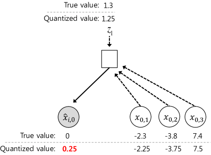
The quantization effect also can cause detection error of the supportive state given $i\notin supp(\mathbf{x}_{0})$, limiting performance of the MAP-approach in the high SNR regime. In order to explain such cases, we provide an example of the measurement message-passing with respect to $x_{0,i}=z_{1}-(x_{0,1}+x_{0,2}+x_{0,3})$ as shown in Fig.7. In this example, we try to find the value of $\widehat{x}_{0,i}$ given $x_{0,1}=-2.3$, $x_{0,2}=-3.8$, $x_{0,3}=7.4$, $z_{1}=1.3$, and $i\notin supp(\mathbf{x}_{0})$, under noiseless setup. Note that in practical operation of the algorithm, the value of each element corresponds to the peak location in the $x$-axis of each density-message. In the sampled-message based BP, the message sampling causes quantization of the values such that we have $Q_{T_{s}}[x_{0,1}]=-2.25$, $Q_{T_{s}}[x_{0,2}]=-3.75$, $Q_{T_{s}}[x_{0,3}]=7.5$, $Q_{T_{s}}[z_{1}]=1.25$ with the step size $T_{s}=0.25$ where $Q_{T_{s}}[\cdot]$ denotes the quantization function. In this case, we can simply infer that this measurement message passes a corrupted value $\widehat{x}_{0,i}=0.25$ which is not matched with $i\notin supp(\mathbf{x}_{0})$. If most of the measurement messages to ${x}_{0,i}$ has such corruption, the marginal posterior of ${x}_{0,i}$ will have the peak at an erroneous location, leading to detection error based on the MAP-approach. The same event can occur given $i\in supp(\mathbf{x}_{0})$. However, the effect is not significant because the case of $i\in supp(\mathbf{x}_{0})$ does not bring about the support detection error. In addition, this type of errors is remarkable particularly in the high SNR regime since such corruption is covered by additive noise when SNR is low. Accordingly, the support detection performance of the MAP-approach shows an error-floor in the high SNR regime.

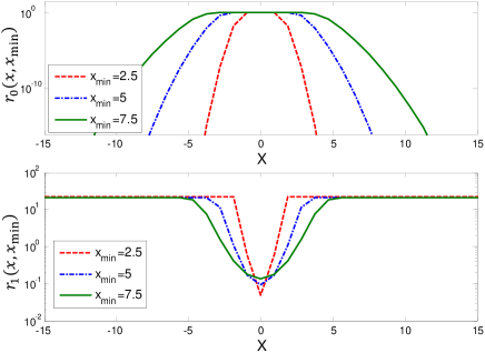
Here, we aim to show how the proposed BHT-detector utilizes the prior knowledge of $x_{min}$ to remove the error-floor of the MAP approach. As we mentioned in Section III-A, we consider the signal model which has $x_{min}$ as a key parameter, according to the result of Wainright et al. [34],[35]. The Wainright’ result revealed that the regulation of $x_{min}$ is imperative for perfect support recovery under noisy setup. This means that we can have additional prior knowledge to the sparse recovery. From (12), the knowledge of $x_{min}$ tells us that there exist no nonzero elements which have value within $|x_{0,i}|<x_{min}$. The BHT-detector reflects $x_{min}$ to calibrate the reference functions. Rather than the functions given in (40), we use its calibrated version given as

$$r_{0}(x,x_{min}) := \frac{{f_{X}(x|S=0;x_{min})}}{{f_{X}(x;x_{min})}},$$

$$r_{1}(x,x_{min}) := \frac{{f_{X}(x|S=1)}}{{f_{X}(x;x_{min})}},$$ (42)

to improve the performance for the Gaussian signal model, where

$$\begin{array}[]{l}f_{X}(x|S=0;x_{min})=\mathcal{N}(x;0,c\,x_{min}),\\ f_{X}(x;x_{min})=qf_{X}(x|S=1)+(1-q)f_{X}(x|S=0;x_{min}),\end{array}$$ (45)

with a constant $c\in\mathbb{R}$. For signed signals, we simply use $x_{min}=c\cdot\sigma_{X_{1}}/2$.

This calibration depresses the weight of $r_{1}(x,x_{min})$ and puts more weight to $r_{0}(x,x_{min})$ over $|x_{0,i}|<x_{min}$, as shown in Fig.8. This implies that the detector excludes elements within $|x_{0,i}|<x_{min}$ from the signal support set. Therefore, we can eliminate the misdetection cases given $i\notin supp(\mathbf{x}_{0})$ such as the example in Fig.7, removing the error-floor in the high SNR regime effectively.

TABLE II: List of sparse recovery algorithms in the experiment

Algorithm	Complexity	Type of $\Phi$	Use of no-
	for recovery		ise statistic
BHT-BP	$O(N\log N+KM)$	sparse-binary	Yes
Standard	$O(N\log N)$	sparse-binary	No
CS-BP
CS-BP-NS	$O(N\log N)$	sparse-binary	Yes
SuPrEM	$O(N\log N)$	sparse-binary	Yes
BCS	$O(NK^{2})$	dense-Gaussian	No
L1-DS	$\Omega(N^{3})$	dense-Gaussian	No

VI Experimental Validation

We support our investigation for the proposed algorithm via experimental validation. We performed two types of the experiments for this validation as given below:

1. SER performance over SNR: To support our claims for support detection based on BHT, we simulate the SER performance, described in (22), as a function of SNR, compared to that of the MAP-approach used in CS-BPs,

2. MSE comparison over SNR: To compare the recovery performance of the recent NSR algorithms listed in Table.II and the oracle estimator, in the presence of noise, we examine MSE performance, described in (23), as a function of SNR.

Here, for SuPrEM, BCS, and L1-DS, we obtained the source codes from each author’s webpage. For CS-BP, we implemented it using the sampled-message based approach and the spike-and-slab prior, making the algorithm into two different versions: 1) the standard CS-BP which is the original by the corresponding papers [18],[19], and 2) CS-BP-NS which utilizes the noise statistic in the BP-iteration. In implementation of the sampled-message based BP for CS-BPs and BHT-BP, we used $N_{d}=256$ such that the sampling step for the density-messages is $T_{s}\approx 0.1172$ with (24). For the choice of the sensing matrix, BHT-BP and CS-BPs were sparse-binary matrices with $L=4$ such that the matrix sparsity is $7.8\%$, as discussed in Section III-A, . L1-DS and BCS are performed with the standard Gaussian matrix having the equal column energy as the sparse-binary matrix, for fairness, i.e., $\left\|{\mathbf{\phi}_{j,Gaussian}}\right\|_{2}^{2}=\left\|{\mathbf{\phi}_{j,Sparse}}\right\|_{2}^{2}=L$. In addition, SuPrEM worked with a sensing matrix generated from a low-density frame [21].

In these experiments, we examined the two types of signal models defined in Section III-B, Gaussian signals and signed signals, with $N=1024$, $q=0.05$, and $\sigma_{X_{1}}=5$. For the case of Gaussian signals, we restricted the magnitude level of the signal elements to $x_{min}\leq|x_{0,i}|\leq 3\sigma_{X_{1}}$ where $x_{min}=\sigma_{X_{1}}/4$. In addition, we fixed the undersampling ratio to $M/N=0.5$ because the focus of this paper is to investigate the behavior of NSR over SNR. Also, we used Monte Carlo method with 200 trials to evaluate the performance in average sense.

Figure 9: SER performance for support detection over SNR for $N=1024$, $q=0.05$, $M/N=0.5$, $\sigma_{X_{1}}=5$, $x_{min}=1.25$, and $N_{d}=256\,(T_{s}\approx 0.1172)$.

VI-A SER Performance over SNR

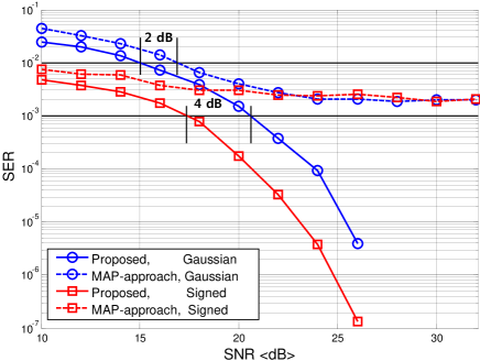
Fig.9 compares a SER performance between the proposed algorithm and the MAP-approach used in CS-BPs, where the BP-process embedded in the both algorithms utilizes the noise statistic. We simulated the SER performance as a function of SNR for the both signal model.

VI-A1 Result at low SNR

In the low SNR regime, the noise-robust property of the proposed BHT-detector provides 2 dB gain at SER = $10^{-2}$ from the the MAP-approach for the Gaussian model, as we discussed in Section V-A. In addition, we note that the case of signed signals shows better performance than the case of Gaussian signals with 4 dB gap at SER = $10^{-3}$. The reason is that in the signed case the nonzero values is fixed to $X_{i\in supp(\mathbf{X})}=\sigma_{X_{1}}$; therefore, the sparse patten of the signal are rarely corrupted by noise and can be detected with less difficulty than the Gaussian case which can have nonzero elements $x_{0,i}<\sigma_{X_{1}}$.

VI-A2 Result at high SNR

As SNR increases, the SER performance of the proposed algorithm shows a waterfall behavior whereas that of the MAP-approach shows an error-floor limited to SER of $2\times 10^{-3}$, for both signal models. In the MAP cases, more SNR cannot help when the curve manifests such an irreducible SER since the level is saturated by quantization effect caused by the sampled-message based BP, as discussed in Section V-B. In contrast, the SER curve of the proposed algorithm declines with more SNR by overcoming quantization effect, removing the error-floor of the MAP-approach for both signal models. Therefore, this result indicates that the proposed BHT-detector can provide the perfect support knowledge to the signal value estimator if sufficient SNR level is present.

Figure 10: MSE comparison over SNR for $N=1024$, $q=0.05$, $M/N=0.5$, $\sigma_{X_{1}}=5$, and $N_{d}=256\,(T_{s}\approx 0.1172)$: Signed signals case.

Figure 11: MSE comparison over SNR for $N=1024$, $q=0.05$, $M/N=0.5$, $\sigma_{X_{1}}=5$, $x_{min}=1.25$, and $N_{d}=256\,(T_{s}\approx 0.1172)$: Gaussian signals case.

VI-B MSE Comparison over SNR

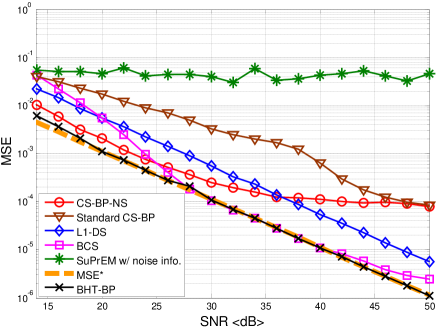
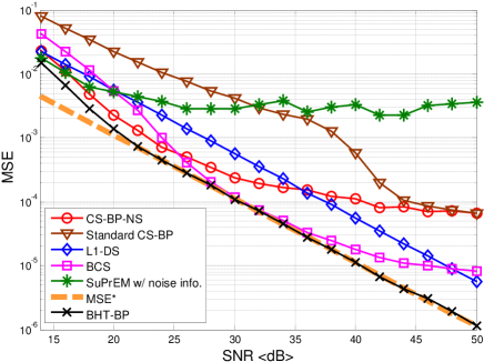
This section provides a MSE comparison among the algorithms in Table.II and the oracle estimator, over SNR, where MSE^∗ denotes the performance of the oracle estimator, given as

$${\text{MSE}}^{*}:=\frac{{{\rm{Tr}}\left[{\left(\frac{1}{{\sigma_{X_{1}}^{2}}}{\bf{I}}+\frac{1}{{\sigma_{N}^{2}}}{{\bf{\Phi}}_{\mathbf{s}}^{T}{\bf{\Phi}}_{\mathbf{s}}}\right)^{-1}}\right]}}{{\left\|{{\bf{x}}_{{{0,\mathbf{s}}}}}\right\|_{2}^{2}}}.$$ (46)

Fig.11 and Fig.11 display the results for the signed signal and the Gaussian signal case respectively.

VI-B1 Result at low SNR

When the measurements are heavily contaminated by noise (below SNR =20 dB), performance of all recovery algorithms is basically degraded. Under such degradation, BHT-BP and CS-BP-NS outperform the others because they are fully employing noise statistic during the recovery process, where difference of BHT-BP and CS-BP-NS (2 dB SNR gap at MSE = $10^{-3}$) is from types of the support detectors as we validated in Section V-A.

The use of noise statistic remarkably affects the performance of BP-based algorithms as discussed in Section IV-A. As a support, the standard CS-BP shows $8\sim 10$ dB SNR loss from CS-BP-NS for the both signal models. For SuPrEM, even if it also includes noise variance as a input parameter, the performance is underperformed since SuPrEM was devised mainly for the $K$-sparse signals which have the support set with fixed cardinality.

As SNR increases, BHT-BP approaches the oracle performance MSE^∗ where the case of signed signal in Fig.11 shows faster approaching than the case of Gaussian signals in Fig.11 with approximately 4 dB gap. we note that this gap according to the signal models is originated from the gap in the SER performance.

VI-B2 Result at high SNR

In the high SNR regime, performance of the algorithms are generally improved except SuPrEM, for the both signal models. Among the algorithms, BHT-BP shows the most closely approaching performance to MSE^∗. This is because the BHT-detector provides the perfect support knowledge beyond a certain SNR level. Although BCS shows a competitive performance within a certain range of SNR (SNR = 28 $\sim$ 40 dB for the signed case, SNR = 30 $\sim$ 34 dB for the Gaussian case), its performance is saturated to a certain level as SNR becomes higher.

For CS-BPs, the use of the noise statistic in the BP-process is no longer be effective beyond a certain SNR level. Indeed, the MSE in Fig.11 and Fig.11 commonly shows that the performance of the standard CS-BP converges to that of CS-BP-NS beyond approximately SNR = 45 dB. In addition, after the convergence the performances are saturated to a certain level even with higher SNR. The cause of this saturation is the quantization effect, as discussed in Section V-B. Using (V-B1), we can calculate the normalized MSE degradation by the quantization under this experimental setup, given as

$$\frac{{T_{s}^{2}/12}}{{{\bf{E}}\left\|{{X_{i\in{\rm{supp}}({\bf{X}})}}}\right\|_{2}^{2}}}=4.5786\times{10^{-5}},$$ (47)

The result in (47) closely lower bounds the MSE of CS-BPs at SNR = 50 dB where the signed and Gaussian cases show MSE = $7.973\times 10^{-5}$ and MSE = $6.554\times 10^{-5}$ respectively. These results exactly explain the performance loss of CS-BPs by quantization effect, standing out BHT-BP to remove the quantization effect using the DD-structure.

VII Conclusion

The theoretical and empirical research in this paper demonstrated that BHT-BP is a powerful algorithm for NSR from a denoising standpoint. In BHT-BP, we employed the DD-structure, which consists of support detection and signal value estimation. The support detector is designed by a combination of the sampled-message based BP and Bayesian hypothesis test (BHT), and the signal value estimation performs in MMSE sense.

We have shown that BHT-BP utilizes the posterior knowledge more efficiently than the MAP-based algorithms, over the entire range of SNR. In the low SNR regime, the BHT-based support detector provides noisy-robust detection against measurement noise. In the high SNR regime, the DD-structure eliminates quantization error due to the sampled-message BP from the signal value estimation. In addition, we applied the knowledge of $x_{min}$ to the proposed algorithm based on the result of Wainright et al. [34],[35]. Then, we showed that the use of $x_{min}$ enables BHT-BP to remove the error-floor of the MAP-based algorithms, inducing the performance to approach that of the oracle estimator as SNR increases.

We supported such advantages of BHT-BP via experimental validation. Our experiments showed that BHT-BP outperforms the other recent NSR algorithms over entire range of SNR, approaching the recovery performance of the oracle estimator as SNR increases.

Appendix I
Fundamentals of Density-message Passing

The goal of BP is to iteratively approximate the marginal posterior densities via a message update rule. The message update rule can have various forms according to applications and frameworks. In the NSR problems, the BP-messages are represented as PDFs since the signal is a real-valued. We refer to such messages passing as density-messages passing. In this appendix, we provide the fundamentals of the density-message passing under the BP-SM framework.

In the discussion here, we consider a random linear model corresponding to (8), given as

$$\mathbf{Z}=\mathbf{\Phi}\mathbf{X}+\mathbf{N},$$ (48)

where $\mathbf{X}$ and $\mathbf{Z}$ are random vectors for $\mathbf{x}_{0}$ and $\mathbf{z}$ respectively, and $\mathbf{N}\sim\mathcal{N}(0,\sigma_{N}^{2}\mathbf{I})$ is a random vector for the Gaussian noise vector $\mathbf{n}$. In addition, we assume that the sensing matrix $\mathbf{\Phi}\in\{0,1\}^{M\times N}$ sufficiently sparse such that the corresponding bipartite graph is tree-like.

Given $\mathbf{Z}=\mathbf{z}$, we can represent the marginal posterior density of $X_{i}$ in the form of ${\rm{Posterior=Prior}}\times\frac{{{\rm{Likelihood}}}}{{{\rm{Evidence}}}}$ using the Bayesian rule, given as

$$f_{X_{i}}(x|\mathbf{Z}=\mathbf{z}) =f_{X}(x)\times\frac{{f_{\mathbf{Z}}({{\bf{z}}|X_{i}=x_{i})}}}{f_{\mathbf{Z}}(\mathbf{z})}$$ (49)

$$\propto f_{X}(x)\times\prod\limits_{j\in N_{\mathcal{V}}(i)}f_{Z_{j}}({z}|X_{i}={x_{i}}),$$ (50)

where we postulate that the measurements associated with $X_{i}$, i.e., $\{{Z_{k}}:k\in{N_{\mathcal{V}}}(i)\}$, are statistically independent given $X_{i}=x_{i}$ [22]-[24] using the tree-like property of $\mathbf{\Phi}$, to move to (50) from (49).

We note each decomposition of the likelihood density, i.e., $f_{Z_{j}}(z|X_{i}={x_{i}})\,\,\forall j\in N_{\mathcal{V}}(i)$ called measurement density, which is associated with the marginal posteriors of elements in $\{{X_{k}}:k\in{N_{\mathcal{C}}}(j),k\neq i\}$. From (48), a measurement $Z_{j}$ is represented by

$$\begin{array}[]{l}{Z_{j}}={X_{i}}+\sum\limits_{k\in{N_{\mathcal{C}}}(j)\backslash\{i\}}{{X_{k}}}+{N_{j}}={X_{i}}+{Y_{j}},\end{array}$$ (52)

where we define $Y_{j}:=\sum\limits_{k\in{N_{\mathcal{C}}}(j)\backslash\{i\}}{{X_{k}}}+{N_{j}}$. Then, by factorizing over $Y_{j}$, the expression of $f_{Z_{j}}(z|X_{i}=x_{i})$ becomes

$${f_{{Z_{j}}}}(z|X_{i}={x_{i}}) ={f_{{Z_{j}}}}(x+y|X_{i}={x_{i}})$$

$$=\int\limits_{{Y_{j}}}{{f_{{Z_{j}}}}(x+y|{X_{i}}=x_{i},{Y_{j}})\underbrace{{f_{{Y_{j}}}}(y|{X_{i}}={x_{i}})}_{={f_{{Y_{j}}}}(y)}dy}$$

$$={f_{{Z_{j}}}}(z|{X_{i}}=x_{i},{Y_{j}})\otimes{f_{{Y_{j}}}}(-y),$$ (53)

where ${f_{{Y_{j}}}}(y|X_{i}=x_{i})={f_{{Y_{j}}}}(y)$ since $Y_{j}$ is independent of $X_{i}$. Since elements in $\{{X_{k}}:k\in N_{\mathcal{C}}(j),k\neq i\}$ and $N_{j}$ are statistically independent given $\mathbf{Z}=\mathbf{z}$ under the tree-like assumption [22]-[24], we may approximately evaluate the PDF of $Y_{j}$ by linear convolution as

$${f_{{Y_{j}}}}(y)=\left(\bigotimes\limits_{k\in N_{\mathcal{C}}(j)\backslash\{i\}}{f_{X_{k}}}(x|\mathbf{Z}=\mathbf{z})\right)\otimes f_{N_{j}}(n).$$ (54)

Finally, by substituting (54) into (Appendix I Fundamentals of Density-message Passing) we obtain the expression of the measurement density given as

$$f_{Z_{j}}(z|X_{i}={x_{i}})=$$

$$\underbrace{f_{Z_{j}}(z|X_{i},Y_{j})}_{=\delta_{z_{j}}}\otimes f_{N_{j}}(n)\otimes\left(\bigotimes\limits_{k\in N_{\mathcal{C}}(j)\backslash\{i\}}{f_{X_{k}}}(-x|\mathbf{Z}=\mathbf{z})\right),$$ (55)

where $f_{N_{j}}(n)=f_{N_{j}}(-n)$ owing to the symmetry shape of Gaussian densities, and $f_{Z_{j}}(z|X_{i},Y_{j})=\delta_{z_{j}}$ is true since no uncertainty on $Z_{j}$ exists given $X_{i},Y_{j}$ which contain information on the neighbored signal elements.

Using the derivation in (50) and (Appendix I Fundamentals of Density-message Passing), we can compose the update rule for the density-message passing. The practical details are provided in Section IV-A, on the basis of the sampled-message approach.

References

- [1] D. L. Donoho, M. Elad, and V. Temlyakov, “Stable recovery of sparse overcomplete representations in the presence of noise,” IEEE Trans. Inf. Theory, vol. 52, no. 1, pp. 6-18, Jan. 2006.
- [2] E. Candes, J. Romberg, and T. Tao, “Stable signal recovery from incomplete and inaccurate measurements,” Comm. Pure Appl. Math., vol. 59, no. 8, pp. 1207-1223, Aug. 2006.
- [3] J. A. Tropp, “Just relax: convex programming methods for identifying sparse signals in noise,” IEEE Trans. Inform. Theory, vol. 52, no. 3, pp. 1030-1051, 2006.
- [4] J. Haupt and R. Nowak, “Signal reconstruction from noisy random projections,” IEEE Trans. Inform. Theory, vol 52, no. 9, 4036-4048, Sep. 2006.
- [5] E. Candes and T. Tao, “The Dantzig selector: statistical estimation when p is much larger than n,” Ann. Statist., vol. 35, no. 6, pp. 2313-2351, 2007.
- [6] R. Tibshirani, “Regression shrinkage and selection via the lasso,” J. Roy. Statisti. Soc., Ser. B, vol. 58, no. 1, pp. 267.288, 1996.
- [7] D. L. Donoho and M. Elad, “Optimally sparse representation in general dictionaries via l1 minimization,” Proc. Nat. Sci. (PNAS), vol. 100, no. 5, pp. 2197-2002, Mar. 2003.
- [8] A. M. Bruckstein, D. L. Donoho, and M. Elad, “From sparse solutions of systems of equations to sparse modeling of signals and images,” SIAM Rev., vol. 51, no. 1, pp. 34.81, Feb. 2009.
- [9] M. E. Tipping, “Sparse Bayesian learning and the relevance vector machine,” J. Mach. Learn. Res., vol. 1, pp. 211-244, 2001.
- [10] D. P. Wipf and B. D. Rao, “Sparse Bayesian learning for basis selection,” IEEE Trans. Signal Process., vol. 52, no. 8, pp. 2153-2164, Aug. 2004.
- [11] Shihao Ji, Ya Xue, and Lawrence Carin, “Bayesian compressive sensing,” IEEE Trans. Signal Process., vol. 56, no. 6, pp. 2346-2356, June. 2008.
- [12] S. Babacan, R. Molina, and A. Katsaggelos, “Bayesian compressive sensing using Laplace priors,” IEEE Trans. Signal Process., vol. 19, no. 1, pp. 53-63, Jan. 2010.
- [13] L. He, L. Carin, “Exploiting structure in wavelet-based Bayesian compressive sensing,” IEEE Trans. Signal Process., vol. 57, no. 9, pp. 3488-3497, Sep. 2009.
- [14] P. Schnitter, L. C. Potter, and J. Ziniel, “Fast Bayesian matching pursuit,” Proc. in Workshop on Inform. Theory and App. (ITA), La Jolla, CA, pp. 326-333, Jan. 2008.
- [15] M. Elad and I. Yavneh, “A plurality of sparse representations is better than the sparsest one alone,” IEEE Trans. Inform. Theory, vol. 55, no. 10, pp. 4701-4714, Oct. 2009.
- [16] M. Protter, I. Yavneh, and M. Elad, “Closed-form MMSE estimation for signal denoising under sparse representation modeling over a unitary dictionary,” IEEE Trans. Signal Process., vol. 58, no. 7, pp. 3471-3484, Jul. 2010.
- [17] J. Kang, H.-N. Lee, and K. Kim, “Message passing aided least square recovery for compressive sensing,” in Proc. in Signal Processing with Adaptive Sparse Structured Representation (SPARS), pp. 124, Jun. 2011.
- [18] S. Sarvotham, D. Baron, and R. Baraniuk, “Compressed sensing reconstruction via belief propagation,” Rice Univ., Houston, TX, Tech. Rep. TREE0601, Jul. 2006.
- [19] D. Baron, S. Sarvotham, and R. Baraniuk, “Bayesian compressive sensing via belief propagation,” IEEE Trans. Signal Process., vol. 58, no. 1, pp. 269-280, Jan. 2010.
- [20] X. Tan and J. Li, “Computationally efficient sparse Bayesian learning via belief propagation,” IEEE Trans. Signal Process., vol. 58, no. 4, pp. 2010-2021, Apr. 2010.
- [21] M. Akcakaya, J. Park, and V. Tarokh, “A coding theory approach to noisy compressive sensing using low density frame,” IEEE Trans. Signal Process., vol. 59, no. 12, pp. 5369-5379, Nov. 2011.
- [22] D. Guo and S. Verd u, “Randomly spread CDMA: Asymptotics via statistical physics,” IEEE Trans. Inform. Theory, vol. 51, no. 6, pp. 1983-2010, Jun. 2005.
- [23] D. Guo and C.-C. Wang, “Asymptotic mean-square optimality of belief propagation for sparse linear systems,” Proc. in IEEE Inform. Theory Workshop, pp. 194-198, Chengdu, China, Oct. 2006.
- [24] D. Guo and C.-C. Wang, “Random sparse linear systems observed via arbitrary channels: a decoupling principle,”Proc. in IEEE Int. Symp. Inform. Theory (ISIT), pp. 946-950, Nice, France, June. 2007.
- [25] G. Guo and C. C. Wang, “Multiuser detection of sparsely spread CDMA,” IEEE J. Sel. Areas Comm., vol. 26, no. 3, pp. 421-431, Mar. 2008.
- [26] T. Tanaka and M. Okada, “Approximate belief propagation, density evolution, and neurodynamics for CDMA multiuser detection,” IEEE Trans. Inform. Theory, vol. 51, no. 2, pp. 700-706, Feb. 2005.
- [27] E. Sudderth, A. Ihler, W. Freeman, and A. S. Willsky, “Nonparametric belief propagation,” MIT, Cambridge, MA, MIT LIDS Tech. Rep. 2551, Oct. 2002.
- [28] N. Noorshams, and M. J. Wainwright, “Quantized stochastic belief propagation: efficient message-passing for continuous state spaces,” Proc. in IEEE Int. Symp. Inform. Theory (ISIT), pp. 1246-1250, July, 2012.
- [29] M. J. Wainwright, T. Jaakkola, and A. Willsky, “Tree-based reparameterization analysis of sum-product and its generalizations,” IEEE Trans. Inform. Theory, vol. 49, no. 5, pp. 1120-1145, May. 2003.
- [30] S. Rangan, “Estimation with random linear mixing, belief propagation and compressed sensing,” Proc. in 44th Annu. Conf. Inform. Sci. and Syst. (CISS), pp. 1-6, Mar. 2010.
- [31] R. G. Gallager, Low-Density Parity Check Codes, MIT Press: Cambridge, MA, 1963.
- [32] D. MacKay, “Good error-correcting codes based on very sparse matrices,”IEEE Trans. Inform. Theory, vol. 45, no. 2, pp. 399-431, Mar. 1999.
- [33] T. Richardson, and R. Urbanke, “The capacity of low-density parity check codes under message-passing decoding,” IEEE Trans. Inform. Theory, vol. 47, no. 2, pp. 599-618, Feb. 2001.
- [34] W. Wang, M. J. Wainwright, and K. Ramchandran, “Information-theoretic limits on sparse signal recovery: Dense versus sparse measurement matrices,” IEEE Trans. Inform. Theory, vol. 56, no. 6, pp. 2967-2979, Jun. 2010.
- [35] M. J. Wainwright, “Information-theoretic limits on sparsity recovery in the high-dimensional and noisy setting,” IEEE Trans. Inform. Theory, vol. 55, no. 12, pp. 5728-5741, Dec. 2009.
- [36] D. Middleton and R. Esposito, “Simultaneous optimum detection and estimation of signal in noise,” IEEE Trans. Inform. Theory, vol. 14, no. 3, pp. 434-444, May. 1968.
- [37] G. Picchi and G. Prati, “Blind equalization and carrier recovery using ”Stop-and-Go” decision-directed algorithm,” IEEE Trans. Commun., vol. 35, no. 9, pp. 877-887, Sep. 1987.
- [38] D. Godard, “Self-recovering equalization and carrier tracking in two-dimensional data communication systems,”IEEE Trans. Commun., vol. 28, no. 11, pp. 1867-1875, Nov. 1980.
- [39] Y. Ephraim and D. Malah, “Speech enhancement using a minimum measure squar error short-time spectral amplitude estimator,” IEEE Trans. Acoust. Speech, and Signal Process. vol. ASSP-32, no. 6, pp. 1109-1121, Dec. 1984.
- [40] H.-N. Lee, Introduction to Compressed Sensing (Lecture notes), Spring Semester, 2011.
- [41] A. Pizurica and W. Philips, “Estimating the probability of the presence of a signal of interest in multiresolution single- and multiband image denoising,” IEEE Trans. Image Process. vol. 15, no. 3, pp. 654-665, Mar. 2006.
- [42] B. Vidakovic, “Nonlinear wavelet shrinkage with Bayes rules and Bayes factors,” J. Amer. Stat. Assoc., vol. 93, pp. 173-179, 1998.
- [43] J. Kang, H.-N. Lee, and K. Kim, “Bayesian hypothesis test for sparse support recovery using belief propagation,” Proc. in IEEE Statistical Signal Processing Workshop (SSP), pp. 45-48, Aug. 2012.
- [44] D. L. Donoho, A. Maleki, and A. Montanari, “Message passing algorithms for compressed sensing,”, Proc. Nat. Acad. Sci., vol. 106, pp. 18914-18919, Nov. 2009.
- [45] D. L. Donoho, A. Maleki, and A. Montanari, “Message passing algorithms for compressed sensing: I. Motivation and construction,” Proc. in IEEE Inform. Theory Workshop (ITW), Cairo, Egypt, Jan. 2010.
- [46] M. Bayati and A. Montanari, “The dynamics of message passing on dense graphs, with applications to compressed sensing,” IEEE Trans. Inform. Theory, vol. 57, no. 2, pp. 764-785, Feb. 2011.
- [47] S. Rangan, “Generalized approximate message passing for estimation with random linear mixing,” Proc. in IEEE Int. Symp. Inform. Theory (ISIT), pp. 2168-2172, Aug. 2011.
- [48] D. L. Donoho, A. Maleki, and A. Montanari, “The noise-sensitivity phase transition in compressed sensing,” IEEE Trans. Inform. Theory, vol. 57, no. 10, pp. 6920-6941, Oct. 2011.
- [49] S. Kay, Fundamentals of Statistical Signal Processing Volume I: Estimation theory, Prentice Hall PTR, 1993.
- [50] S. Kay, Fundamentals of Statistical Signal Processing Volume II: Detection theory, Prentice Hall PTR, 1993.
- [51] Ake Bjorck, Numerical Methods for Least Squares Problems,,SIAM: PA, 1996.
- [52] F. Pukelsheim, “The three sigma rule,” The American Statistician, vol. 48, no. 2, May. 1994.
- [53] H. Ishwaran and J. S. Rao, “Spike and slab variable selection : Frequentist and Bayesian strategies,” Ann. Statist., vol.33, pp. 730-773, 2005.