Entanglement and area laws in weakly correlated gaussian states
Abstract
We examine the evaluation of entanglement measures in weakly correlated gaussian states. It is shown that they can be expressed in terms of the singular values of a particular block of the generalized contraction matrix. This result enables to obtain in a simple way asymptotic expressions and related area laws for the entanglement entropy of bipartitions in pure states, as well as for the logarithmic negativity associated with bipartitions and also pairs of arbitrary subsystems. As illustration, we consider different types of contiguous and noncontiguous blocks in two dimensional lattices. Exact asymptotic expressions are provided for both first neighbor and full range couplings, which lead in the first case to area laws depending on the orientation and separation of the blocks.
pacs:
03.67.Mn, 03.65.Ud, 05.30.JpI Introduction
Entanglement is a valuable resource that plays a key role in quantum information processing and transmission based on qubits NC.00 ; BB.93 ; JL.03 ; RB.01 or on continuous variable systems WP.12 . It has also provided new insights into the role of quantum correlations in the critical behavior of many-body quantum systems OA.02 ; ON.02 ; VLRK.03 ; AFOV.08 ; ECP.10 . Nonetheless, the evaluation of genuine quantum correlations for a given state of a many-body system is in general a difficult task. On the one hand, rigorous computable entanglement measures exist just for pure states, where the entanglement entropy, i.e. the entropy of the reduced state of a subsystem, provides the basic measure of bipartite entanglement BBPS.96 . In the case of mixed states, rigorous measures like the entanglement of formation BVSW.96 , which is the convex-roof extension of the previous measure RC.03 , involve a minimization over a very high dimensional space of parameters and are therefore not directly computable. This has turned the attention to the negativity VW.02 , or equivalently, the logarithmic negativity VW.02 ; Pl.05 , which quantifies the violation of the positive partial transpose separability criterion by entangled states and is a bipartite entanglement monotone VW.02 , computable in principle for any bipartition in any pure or mixed state. Nevertheless, the accurate evaluation of these quantities demands a deep knowledge of the many body state, which requires in general an amount of information which increases exponentially with the system size. This fact limits the possibility of closed evaluations to states characterized by a manageable number of parameters AFOV.08 .
A prime example of such states are the gaussian states, i.e., ground or thermal states of stable gapped Hamiltonians quadratic in boson operators, or equivalently generalized coordinates and momenta WP.12 ; HSH.1999 ; RS.00 . For such states, of crucial importance for continuous variable quantum information WP.12 , the entanglement entropy of bipartitions of pure states and the negativity between arbitrary subsystems in pure or mixed states can be evaluated in terms of the elements of the covariance matrix AEPW.02 ; CEPD.06 ; CEP.07 ; ASI.04 ; AI.08 , i.e., of the generalized contraction matrix of pairs of boson operators RS.80 ; MRC.10 . However, even in this scenario, the extraction of analytic expressions for these quantities for arbitrary subsystems is in general not straightforward AEPW.02 ; CEPD.06 ; MRPR.09 .
The aim of this work is to discuss the evaluation of the previous measures in weakly correlated gaussian states, such as typical ground states of gapped hamiltonians, which can be characterized by excitations over a product state. Gaussian states are usually described in terms of the phase space formalism WP.12 , which allows to connect their entanglement properties with correlations in phase space. Here we will consider a different approach, based on the Fock representation, which provides an equivalent yet in many cases more clear way to evaluate and represent entanglement measures MRC.10 . We will show that the entanglement entropy and negativity can be expressed in terms of the singular values of sub-blocks of basic contraction matrices, which can be evaluated analytically in the perturbative limit for some typical couplings. The formalism also allows the straightforward derivation of area laws ECP.10 ; CEPD.06 ; CC.04 ; JK.04 ; LORV.05 for these quantities. The emergent area laws for the entanglement entropy and negativity are different, i.e., they depend on distinct measures of the boundary size, and are affected by the orientation and separation of the subsystems. Let us also remark that the ground state of weakly interacting spin systems can also be described by gaussian states through different approximate bosonization techniques RS.80 ; MRC.10 ; RCM.11 , entailing that the scope of the present scheme is quite general.
The formalism is described in section II, while section III considers its application to specific systems, essentially ground states of two dimensional lattices with short range couplings, although the full range case is also considered. The present scheme allows to easily obtain exact analytic asymptotic expressions for the entanglement entropy and logarithmic negativity of different types of bipartitions and block pairs, both contiguous and separated, which will be compared with exact numerical results. They clearly show the emergence of precise area laws. Conclusions are finally drawn in IV. We also include appendices containing the details of the perturbative expansion for the symplectic eigenvalue problem and the evaluation of singular values.
II Formalism
II.1 Entanglement entropy and negativity in Gaussian states
The class of Gaussian states in a bosonic system can be defined as those states of the form
| (1) |
where is a positive definite quadratic form on boson operators , (, ),
| (4) | |||||
with , and is a displacement operator (). In (4), is the diagonal matrix of local bare energies and are the coupling strengths between pairs of different bosons (, ). In the pure state limit , , with the ground state of . The displacements can be taken into account by local shifts , so that in what follows we will set , such that .
The key property of these states is that by means of Wick’s theorem RS.80 , the expectation value of any bosonic operator (and hence ) is fully determined by the displacements and the generalized contraction matrixMRC.10 ; RS.80
| (7) | |||||
| (8) |
where is the symplectic metric and , .
We may diagonalize or by means of a symplectic transformation satisfying , corresponding to a Bogoliubov transformation to boson operators , such that , with diagonal (, ). This leads to the standard diagonalization of the matrix (as ). The matrix can be written in block form as
| (9) |
where and should satisfy
| (10a) | |||||
| (10b) | |||||
The blocks of the contraction matrix acquire then a simple form in terms of , and the diagonal block :
| (11a) | |||||
| (11b) | |||||
For a pure state, and Eqs. (11) lead to , , implying
| (12) |
For such states, the entanglement between any subsystem and its complement can be measured through the von Newmann entropy of any of the reduced states:
| (13) |
where . In a Gaussian state, the validity of Wick’s theoremRS.80 implies that the state of any subsystem is also Gaussian and hence fully characterized by the corresponding contraction matrix , which is just the sub-block of with indexes belonging to :
| (16) |
The von Newmann entropy (13) can then be expressed in terms of the symplectic eigenvalues of as
| (17) |
In the case of a mixed state or for pairs of non-complementary subsystems , the subsystem entropy is no longer a measure of quantum correlations. Instead, a well known computable entanglement monotone for such systems is the negativity VW.02 , which is just the sum of the negative eigenvalues of the partial transpose . An associated quantity is the logarithmic negativity
| (18) |
where denotes the trace norm. For a gaussian state, can be expressed in terms of the negative symplectic eigenvalues of the contraction matrix determined by , with blocks
| (19) |
where denotes the matrix of elements with and , and . Eq. (18) then becomes
| (20) |
We notice that MRC.10 . In the case where and , Eq. (20) can be expressed in terms of the symplectic eigenvalues of as MRC.10
| (21) |
which, like Eq. (13), is again a concave function of the .
II.2 Weakly correlated pure Gaussian states
We consider now the case of weakly correlated pure Gaussian states, i.e., states in which the local symplectic eigenvalues (those corresponding to a single mode )
| (22) |
satisfy , such that each mode is weakly entangled with the rest of the system. In the local basis where (this implies replacing , with and the phase of ), and weak coupling implies, together with the positivity of and , that , . In this limit, Eqs. (11)–(12) then lead, neglecting terms , to
| (23) |
which for a subsystem implies
| (24) |
Using Eq. (24) and the results of Appendix A, the symplectic eigenvalues of will then agree at this order with the standard eigenvalues of the matrix
| (25) |
which are just the square of the singular values of (see Appendix B). We then obtain, at this order,
| (26) |
Entanglement depends at this level just on the contractions between and . For instance, in the case of a single site , Eq. (26) implies .
In this regime we may just set in Eq. (17), such that the entanglement entropy becomes
| (27) |
Considering now the negativity, in the present regime the symplectic eigenvalues of will be given at leading order by the eigenvalues of (see Appendix A)
| (30) |
where, for or ,
| (31) |
For pure global states, Eq. (25) leads to , indicating that takes into account the correlations with the environment of . Up to first order in , we may neglect its second order effect in and in (30), such that
| (32) |
depend just on the correlation with the environment of . If the sites of and correlated with each other have correlations of the same order (or less) with , (i.e. and of the same order as , at least for the subsets of and mutually correlated) we can directly neglect and in Eq. (30) at order . The negative symplectic eigenvalues of will then be given by minus the singular values of (see Appendix B):
| (33) |
which depend again just on the contractions between and . For instance, this is the case of contiguous blocks in a scenario of short range couplings, and also that where is the complement of ().
In the general case, however, the whole matrix (30) should be diagonalized. First order corrections lead to
| (34) |
where , are the diagonal elements in the local basis of and where (see App. B). As and are positive matrices in the approximations (31)–(32), negative eigenvalues can only arise if and are not much larger than . A sufficient condition ensuring a negative eigenvalue of (30) is
| (35) |
II.3 Ground state correlation matrix in the weakly interacting case
A particular case of the previous results arises when we deal with the ground state of a Hamiltonian of the form (4). For weak couplings , the diagonalizing symplectic transformation such that , with , can be evaluated perturbatively. At leading order (see Appendix A) the block in (9) is a unitary matrix that diagonalizes , while
| (37) |
Note that, in contrast with the conventional perturbation theory, a possible degeneracy in the local energies will not spoil this result if the system is stable ( ). Notice, however, that can depart considerably from the identity if the are degenerate.
If all local bare energies are nearly equal (), and if energy corrections arising from are neglected (), Eq. (37) reduces to . In such a case, Eq. (11) leads to
| (38) |
with given by Eq. (23). In this regime, correlations are hence proportional to the pairing couplings , decreasing as for increasing local energies. Noteworthy, the strength of the hopping interaction does not affect the ground state correlations at this order. When non degenerate, it just affects dressing the bare pairing interactions.
In the same way, for a common local bare energy , inclusion of second order terms in the couplings leads to
| (39) |
This expression is useful in the present scheme when the first order term vanishes (modes unconnected by ). As the counter terms and in (34) will be of second order in (Eq. (32)), subsystems unconnected by but connected at second order through Eq. (39) may exhibit an non-zero negativity if Eq. (35) holds.
II.4 Area laws
The formulation of the area law for systems with local interactions starts with the definition of a suitable measure for the size of the boundary of the subsystem CEPD.06 ; MRPR.09 ; ECP.10 . An example of such measure is given by the number of pairs of first neighbor modes, with one mode belonging to and the other to . If we define the matrix with entries if modes and are first neighbors and 0 otherwise, that measure can be written as
| (40) |
where is the number of first neighbors of mode in . For the ground state of a gapped bosonic system with constant and isotropic first neighbor interactions , Eq. (38) implies and Eqs. (26)–(27) lead then to
| (41) |
at leading order in , which coincides exactly with the result in CEPD.06 for non critical harmonic systems.
The logarithmic negativity presents, however, a slightly different behavior: for contiguous subsystems, the same procedure and Eqs. (33)–(36) lead to
| (42) |
where the boundary measure is now
| (43) |
with the singular values of the matrix (in comparison, ). If each site in has at most one neighbor in (the opposite may not hold), the rows of will be orthogonal and the singular values will be , leading to
| (44) |
which will differ from (40) if . In general, Eq. (44) may provide a rough approximation to the area (43). Interestingly, in an isotropic hypercubic lattice in dimensions, the approximation (44) is just proportional to the euclidean area for large planar surfaces, both parallel and tilted (with an angle of with respect to the principal axes of the lattice), which is not true in the tilted case neither for nor (see next section).
In general, for two contiguous subsystems , , previous expressions generalize to
| (45) |
at leading order in , where
| (46) |
is a measure of the contacting area between and . Again, if each mode in is linked with at most one mode in , , where is the number of first neighbors of in .
Previous geometric-like expressions can of course be also applied to a general constant coupling , where if pairs are linked by the coupling and otherwise, leading to effective areas and . On the other hand, they cannot be directly applied to higher order effects, like those depending on Eq. (39), as discussed in the next section.
III Examples and asymptotic expressions
We will now use the present formalism to obtain analytic asymptotic expressions for and for typical subsystems , and of a two-dimensional lattice, which will be compared with the exact numerical results and the estimations (41)–(45). We first consider the ground state of a bosonic square lattice with attractive first neighbor couplings
where denotes the unit vector along the axis. We have considered in Figs. (1–6) the isotropic case , with , and a uniform single mode energy . Away from the critical point (where, for fixed , the lowest energy vanishes), the system is gapped and a finite correlation length is expected. Approximately, (exact result for the cyclic case MRC.10 ).
III.1 Entanglement between complementary subsystems
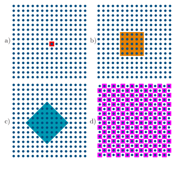
We first consider the four global bipartitions depicted in Fig. 1. Eqs. (26), (33) and (38) lead to analytic asymptotic expressions for the corresponding singular values . At lowest order, their number is just the number of sites at the border. Defining the basic single link singular values
in the case of a single site (Fig. 1a) we obtain
| (47) |
In the rectangular block 1b (parallel to the principal axes), there are three different singular values, corresponding to the horizontal and vertical sides and the four corners, given below with their multiplicity:
| (48) |
In the square block 1c tilted with respect to the principal axes, we obtain, by means of a discrete Fourier transform and neglecting corner effects (see Eq. (85)),
| (49) |
where and is the number of sites at the border. Corner effects will affect essentially just 4 of these eigenvalues with corrections.
Finally, in the checkerboard partition 1d, an exact analytic expression for the singular values is available in the cyclic case again by means of a discrete Fourier transform (see Eq. (41) in RCM.11 ):
| (50) |
where with , .
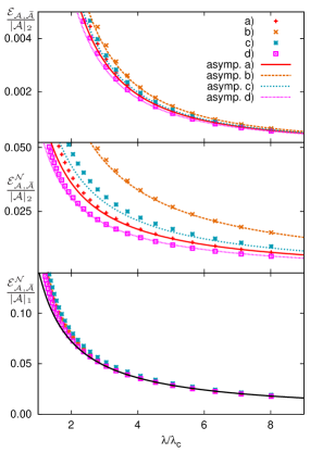
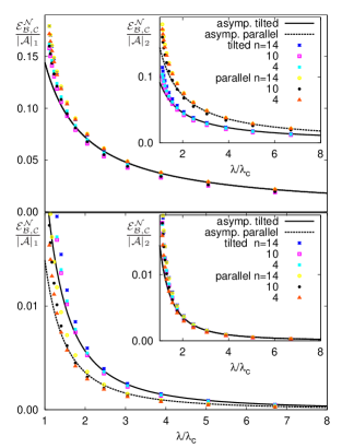
These expressions, together with Eqs. (26), (27), (33) and (36), allow to easily obtain the asymptotic values of the entanglement entropy and negativity of the present bipartitions for large and . For instance, in the isotropic case considered in the figures, setting and neglecting corner and border effects (which just add terms of relative order ), we obtain
| (51a) | |||||
| (51b) | |||||
| (51c) | |||||
| (51d) | |||||
for the entanglement entropy of the single mode, the parallel and tilted square blocks and the checkerboard of Fig. 1. We have replaced sums over in – by integrals (). Note that in the chekerboard case the entanglement entropy scales with the “volume” of rather than the “area” , since all links are broken by the partition (maximally entangled bipartition RCM.11 ).
The corresponding values of the scaled logarithmic negativity are
| (52a) | |||||
| (52b) | |||||
| (52c) | |||||
| (52d) | |||||
The last expressions in (51)–(52) indicate the way to read them. They are of the form
| (53) | |||||
| (54) |
where is the number of modes at the border of (), is the number of connections with the environment per mode at the border (), i.e., the number of links per mode broken by the partition, and , , with , , are geometric correction factors for the tilted () and checkerboard cases ( for the single mode and parallel square). We can easily identify from (53)–(54) the boundary measures of Eqs. (41)–(42):
| (55) |
Comparison with the exact numerical results (Fig. 2) indicate that all these asymptotic expressions are actually quite accurate already for . The scaling of with the area rather than is clearly verified. Moreover, this scaling is more accurate than that of the entanglement entropy with , since the latter contains in an additional geometric correction (Eq. (53)), not comprised in (41). Note also that in the case of the tilted block, and are, respectively, larger and smaller () than the geometric perimeter .
We may also rapidly determine with Eqs. (48) and (53)–(54) the corner effects in case 1b. The actual asymptotic expressions for the finite parallel block are
| (56) | |||||
| (57) |
where the first term is proportional to the number of sites at the border, , and the second represents the positive correction arising from the four corners, reflecting their increased coupling with the environment .
III.2 Non-complementary subsystems
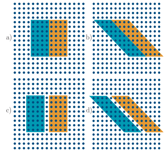
Let us now consider the non-complementary subsystems of Fig. 3. For contiguous parallel blocks contacting at sites, has identical singular values
| (58) |
In the case of contiguous blocks with contacting surfaces tilted with respect to the principal axes, we obtain, neglecting edge effects, the same expression (49) for the , with replaced by the number of contacting sites and . In the isotropic case we then obtain, using Eqs. (33)–(36),
| (59) | |||||
| (60) |
for the logarithmic negativity of parallel and tilted contiguous blocks, which are clearly of the form (54) or (42): and respectively. Tilted boundary surfaces exhibit a larger entanglement per contacting site due to the increased connectivity.
In the case of blocks separated by one site, we should use instead the full Eq. (34) with the second order expression (39). For parallel blocks with sites at separation , the negative eigenvalues of the matrix (30) become, neglecting edge effects and setting ,
| (61) |
For blocks separated by one site through a tilted surface of modes, a discrete Fourier transform leads, neglecting edge effects, to (see Eq. (85))
| (62) | |||||
where , and denotes the expression (49) for . In the isotropic case, Eq. (62) becomes just . For the parallel and tilted subsystems – of Fig. 3 we then obtain, replacing sums by integrals and assuming ,
| (63a) | |||||
| (63b) | |||||
Hence, the logarithmic negativity of the tilted case is, remarkably, twice that of parallel blocks when separated by one site, instead of as in the contiguous case (Fig. 4). Since they are a second order effect, Eqs. (63) are not of the form (54) but rather
| (64) |
if is again the number of connections with the environment per mode. They scale, therefore, with the measure (Fig. 5). For larger separations the negativity vanishes at second order in , as will be of higher order while the counter terms and remain of second order for sites at the surface. Consequently, the negativity becomes vanishingly small for .
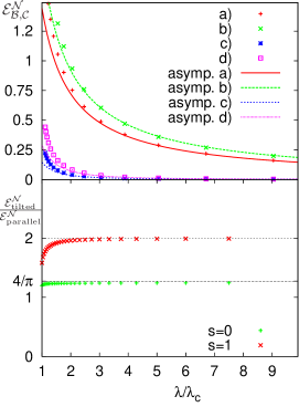
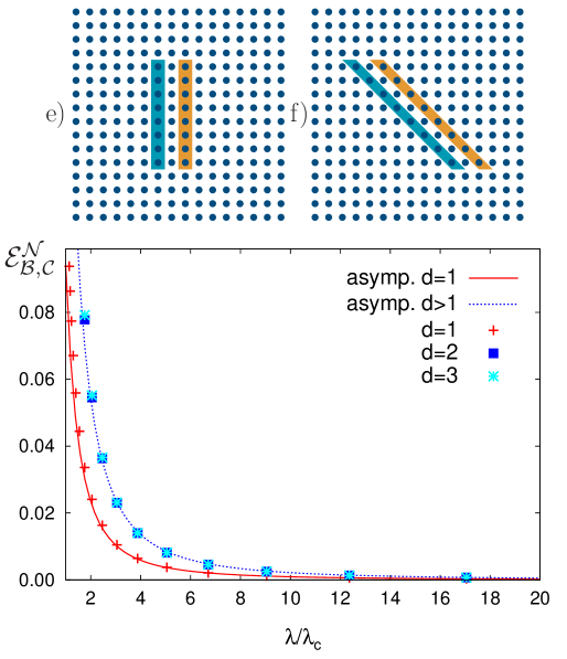
We finally remark that previous expressions are independent (at leading order) of the width of the blocks (assumed finite), provided . In the case of two lines (, Fig. 6), the extra interaction with the environment at the other side of the line leads to an additional negative second order contribution in Eq. (35). Hence, while it can be neglected in the case of contiguous lines, it will double the negative term in Eqs. (63) in the case of lines separated by one site, leading to the lower values
| (65a) | |||||
| (65b) | |||||
which are now valid for . In this case negativity will vanish at second order if . Edge effects in Eqs. (63)–(65) are also of second order and lead, using Eq. (34), to a negative correction .
All present expressions can be directly extended to three dimensions if present subsystems are extended parallel-wise along the axis, replacing by .
III.3 The fully connected case
The evaluation of singular values is also straightforward in the opposite case of a fully and uniformly connected system of modes BDV.06 ; WVB.10 ; MRC.082 ; MRC.10 (LMG type model RS.80 ), where
| (66) |
Here we can also compare with full exact results, since it is exactly and analytically solvable WVB.10 ; MRC.10 . The present system can be used to describe entanglement between systems whose separation is small in comparison with the correlation length.
In the present case, the matrices are obviously constant for , i.e.,
| (67) |
and the entanglement between disjoint subsystems and will just depend on the number of sites in and in , being independent of their separation or shape.
The matrix will then have just a single non-zero singular value disjoint , namely (see Appendix)
| (68) |
In the approximation (26) we then obtain a single non-zero symplectic eigenvalue for any global bipartition ,
| (69) |
where , leading to
which corresponds to an area in (41) (here for ).
Similarly, we obtain a single negative symplectic eigenvalue for any pair of subsystems , given by (68) or, in the complete approximation (30)–(34), by
| (70) |
with . The second term in (70) becomes important for small subsystems in a large environment (). Otherwise it can be neglected, in which case (70) corresponds to in (42)–(45). For the scaling (66), is proportional to , so that Eqs. (68)–(70) remain finite for large . The scaling is then again as in Eqs. (53)–(54) with , and for global partitions or for a pair of subsystems.
The previous picture is, remarkably, also that of the exact treatment, where there is a single non-zero symplectic eigenvalue for any subsystem , given by
| (71) |
(see ref. MRC.10 and Appendix C). Here we have used the local basis where in Eq. (66), in which case Eq. (12) leads to
A first order expansion of (71) in leads then to , which coincides with Eq. (69) since for weak coupling .
In the same way, the exact partial transpose of has a single negative symplectic eigenvalue MRC.10
| (72) |
where , (see appendix C). Expansion of (72) up to first order in leads then exactly to Eq. (70) setting . The present approximate scheme allows then to immediately determine the weak coupling expressions (69)–(70) and to rapidly identify their behavior with sizes , , . The exact value of (to be inserted in (71)–(72)) is given in the appendix (Eq. (86)). Up to first order in we obtain .
IV Conclusions
We have shown how entanglement properties of weakly correlated gaussian states can be recast in terms of the singular values of a sub-block of the generalized contraction matrix associated with the state. This allows to obtain in a quite simple way analytic expressions for both the entanglement entropy between complementary subsystems and the logarithmic negativity for non complementary subsystems, which imply distinct area laws for these two quantities in the case of short range or constant couplings. Several illustrative examples were considered, which show the dependence of these laws on the geometry, connectivity and separation between the subsystems. A final comment is that through application of the bosonic RPA formalism MRC.10 ; RCM.11 ; MRC.08 or other bosonization treatments, WVB.10 ; RS.80 , the present scheme can be applied to weakly interacting spin systems. Moreover, it can in principle be also implemented in phases exhibiting symmetry-breaking at the mean field level (i.e., fields below the critical field in attractive or chains) away from the critical field, provided the proper multiplicity corrections accounting for the different degenerate mean fields MRC.10 is taken into account. Such application is currently being investigated.
The authors acknowledge support of CONICET (NC,JMM) and CIC (RR) of Argentina.
Appendix A Perturbative expansions for the symplectic eigenvalue problem
In this work we have used perturbative results which are not necessarily trivial and which can be obtained following techniques similar to those employed in the perturbative diagonalization of the Dirac equation. We start with the symplectic diagonalization of the contraction matrix of a subsystem , which leads to the system
| (73) | |||||
| (74) |
where is the symplectic eigenvector associated with the eigenvalue . Eq. (74) allows to write as
| (75) |
Replacing (75) in (73) leads to the equivalent non-linear reduced diagonalization problem
For small , in agreement with the hypothesis that the state is weakly correlated, the symplectic eigenvalues are small. Hence, at leading order and we obtain the reduced standard eigenvalue equation
| (76) |
which leads to Eq. (25) and implies Eq. (30). If is the whole system and the latter is assumed to be in the ground state of , all vanish and the relation (Eq. (23)) is obtained.
Let us now consider the Hamiltonian (4). The symplectic diagonalization of entails the standard diagonalization of and leads to the system
| (77) | |||||
| (78) |
In this case, is considered small. For a positive eigenvalue, the zero order approximation is obtained by neglecting all terms proportional to and , which are assumed small in comparison with , and . It leads to , which is a standard hermitian eigenvalue equation for . We then obtain
| (79) | |||||
| (80) |
(Eq. (37)), where we have written , with the diagonal matrix of eigenvalues. It should be noticed that if is degenerate, will affect considerably even if small. Ground state entanglement will remain however small since it depends on . It can be also easily seen that expansion of Eq. (79) up to second order in leads to Eq. (39).
Appendix B Singular values
The singular values of an arbitrary matrix are the square root of the non-zero eigenvalues of or equivalently , which are both positive matrices with the same non-zero eigenvalues. The singular value decomposition implies the existence of unitary matrices , such that , with a diagonal matrix with diagonal elements or , and , unitary eigenvector matrices of and : , , i.e., , for the non-zero eigenvalues , with . For an hermitian , , with the (non-zero) eigenvalues of .
The singular values determine the matrix norm of used in this work, defined as
| (81) |
is the trace norm, the standard Hilbert-Schmidt norm and the spectral norm, which is just the largest singular value.
The singular values of also determine the non-zero eigenvalues of the hermitian matrix
| (82) |
which are , since has eigenvalues . Eigenvalues correspond to normalized eigenvectors , with , and , .
Appendix C Evaluation of singular values
In the first order approximation (38), the matrix for first neighbor couplings and disjoint contiguous blocks , with contacting sites, has elements of the form
| (83) |
if the sites are adequately ordered, where for parallel and for tilted blocks.
For blocks separated by one site, we should use the second order approximation (39), which leads again to a matrix of the form (83), with for parallel blocks and for tilted blocks. In all previous cases, is an hermitian matrix with elements of the form
| (84) |
if edge effects are neglected, where . Such matrix can then be exactly diagonalized (neglecting edge effects) by a discrete Fourier transform MRC.082 , leading to eigenvalues , where and is its dimension (this result is exact if ). For real , as in the previous cases, we then obtain
| (85) |
which leads to Eqs. (49)–(62) (in the case of with the tilted block, the final matrix is again of the form (84)).
In the fully connected case, the exact singular values (68) arise immediately as the matrix is just a rank 1 constant matrix, i.e., , which therefore has a unique non-zero singular value : is a rank 1 matrix with constant elements , whose unique non-zero eigenvalue is due to trace conservation.
The full exact symplectic diagonalization can also be performed (see appendix in MRC.10 for details). We quote here that the exact symplectic eigenvalues of the reduced state of sites for the couplings (66) are and ( fold degenerate). For a pure global state, . In the local basis where , this implies , which leads to Eq. (71). In the same way, we obtain Eq. (72). The exact value of the present was also evaluated in MRC.10 in terms of a parameter ():
| (86) |
where , and , with .
References
- (1) M. A. Nielsen, I. L. Chuang, Quantum Computation and Quantum Information (Cambridge Univ. Press, Cambridge UK, 2000).
- (2) C.H. Bennett et al, Phys. Rev. Lett. 70, 1895 (1993).
- (3) R. Josza and N. Linden, Proc. R. Soc. A 459, 2011 (2003); G. Vidal, Phys. Rev. Lett. 91, 147902 (2003).
- (4) R. Raussendorf and H.J. Briegel, Phys. Rev. Lett. 86, 5188 (2001); R. Raussendorf, D.E. Browne and H.J. Briegel, Phys. Rev. A 68, 022312 (2003).
- (5) C. Weedbrook et al, Rev. Mod. Phys. 84, 621 (2012).
- (6) A. Osterloh, L. Amico, G. Falci, and R. Fazio, Nature (London) 416, 608 (2002).
- (7) T.J. Osborne, M.A. Nielsen, Phys. Rev. A 66, 032110 (2002).
- (8) G. Vidal, J.I. Latorre, E. Rico, and A. Kitaev, Phys. Rev. Lett. 90, 227902 (2003).
- (9) L. Amico, R. Fazio, A. Osterloh, and V. Vedral, Rev. Mod. Phys. 80, 517 (2008).
- (10) J. Eisert, M. Cramer, and M. B. Plenio, Rev. Mod. Phys. 82, 277 (2010).
- (11) C.H. Bennett, H.J. Bernstein, S. Popescu, and B. Schumacher, Phys. Rev. A 53, 2046 (1996).
- (12) C.H. Bennett, D.P. DiVincenzo, J.A. Smolin, W.K. Wootters, Phys. Rev. A 54, 3824 (1996).
- (13) P.Rungta, C.M. Caves, Phys. Rev. A 67 012307 (2003); P. Rungta et al, Phys. Rev. A 64 042315 (2001).
- (14) G. Vidal, R. F. Werner, Phys. Rev. A 65, 032314 (2002).
- (15) M.B. Plenio, Phys. Rev. Lett. 95, 090503 (2005).
- (16) A. S. Holevo, M. Sohma, and O. Hirota, Phys. Rev. A 59, 1820 (1999).
- (17) R. Simon, Phys. Rev. Lett. 84, 2726 (2000).
- (18) K. Audenaert, J. Eisert, M. B. Plenio, and R. F. Werner, Phys. Rev. A 66, 042327 (2002).
- (19) M. B. Plenio, J. Eisert, J. Dreißig, and M. Cramer, Phys. Rev. Lett. 94, 060503 (2005); M. Cramer, J. Eisert, M. B. Plenio, and J. Dreißig, Phys. Rev. A 73, 012309 (2006).
- (20) M. Cramer, J. Eisert, and M. B. Plenio, Phys. Rev. Lett. 98, 220603 (2007).
- (21) G. Adesso, A. Serafini, and F. Illuminati, Phys. Rev. Lett. 93, 220504 (2004); Phys. Rev. A 70, 022318 (2004); A. Serafini, G. Adesso, and F. Illuminati, Phys. Rev. A 71, 032349 (2005).
- (22) G. Adesso, F. Illuminati, Phys. Rev. A 78, 042310 (2008).
- (23) P. Ring and P. Schuck, The Nuclear Many-Body Problem (Springer, NY, 1980).
- (24) J. M. Matera, R. Rossignoli, and N. Canosa, Phys. Rev. A 82 052332 (2010).
- (25) S. Marcovitch, A. Retzker, M. B. Plenio, and B. Reznik, Phys. Rev. A 80, 012325 (2009).
- (26) P. Calabrese and J. Cardy, J. Stat. Mech.: Theory Exp. (2004), P06002.
- (27) V.E. Korepin, Phys. Rev. Lett. 92 096402 (2004); B. -Q. Jin and V.E. Korepin, J. Stat. Phys. 116, 79 (2004).
- (28) J.I. Latorre, R. Orús, E. Rico, and J. Vidal, Phys. Rev. A 71, 064101 (2005).
- (29) R. Rossignoli, N. Canosa, and J. M. Matera, Phys. Rev. A 83, 042328 (2011).
- (30) T. Barthel, S. Dusuel, and J. Vidal, Phys. Rev. Lett. 97, 220402 (2006); J. Vidal, S. Dusuel, T. Barthel, J. Stat. Mech.: Theory Exp. (2007) P01015.
- (31) H. Wichterich, J. Vidal, and S. Bose, Phys. Rev. A 81, 032311 (2010).
- (32) J. M. Matera, R. Rossignoli, and N. Canosa, Phys. Rev. A 78, 012316 (2008).
- (33) J. M. Matera, R. Rossignoli, and N. Canosa, Phys. Rev. A 78, 042319 (2008).