The SEGUE K giant survey II: A Catalog of Distance Determinations for the SEGUE K giants in the Galactic Halo
Abstract
We present an online catalog of distance determinations for K giants, most of which are members of the Milky Way’s stellar halo. Their medium-resolution spectra from SDSS/SEGUE are used to derive metallicities and rough gravity estimates, along with radial velocities. Distance moduli are derived from a comparison of each star’s apparent magnitude with the absolute magnitude of empirically calibrated color-luminosity fiducials, at the observed color and spectroscopic . We employ a probabilistic approach that makes it straightforward to properly propagate the errors in metallicities, magnitudes, and colors into distance uncertainties. We also fold in prior information about the giant-branch luminosity function and the different metallicity distributions of the SEGUE K-giant targeting sub-categories. We show that the metallicity prior plays a small role in the distance estimates, but that neglecting the luminosity prior could lead to a systematic distance modulus bias of up to 0.25 mag, compared to the case of using the luminosity prior. We find a median distance precision of 16%, with distance estimates most precise for the least metal-poor stars near the tip of the red-giant branch. The precision and accuracy of our distance estimates are validated with observations of globular and open clusters. The stars in our catalog are up to 125 kpc distant from the Galactic center, with 283 stars beyond 50 kpc, forming the largest available spectroscopic sample of distant tracers in the Galactic halo.
1 Introduction
Giants of spectral type K have long been used to map the Milky Way’s stellar halo (Bond 1980; Ratnatunga & Bahcall 1985; Morrison et al. 1990, 2000; Starkenburg et al. 2009). In contrast to blue horizontal-branch (BHB) and RR Lyrae stars, giant stars are found in predictable numbers in old populations of all metallicities; and at the low metallicities expected for the Milky Way’s halo they are predominantly K giants. At the same time, their high luminosities ( to ) make it feasible to study them with current wide-field spectroscopic surveys to distances of kpc (Battaglia 2007). The Sloan Extension for Galactic Understanding and Exploration (SEGUE: Yanny et al. 2009), which now has been extended to include SEGUE-2 (Rockosi et al. in prep.) specifically targeted K giants for spectroscopy as part of the effort to explore the outer halo of the Galaxy. For simplicity, henceforth we refer to SEGUE and SEGUE-2 collectively as simply SEGUE. The SEGUE data products include sky positions, radial velocities, apparent magnitudes, and atmospheric parameters (metallicities, effective temperatures, and surface gravities), but no preferred distances.
Distance estimates to kinematic tracers, such as the K giants, are indispensable for studies of Milky Way halo dynamics, such as estimates of the halo mass (Battaglia et al. 2005; Xue et al. 2008), for exploring the formation of our Milky Way (e.g., probing velocity-position correlations, Starkenburg et al. 2009; Xue et al. 2011), and for deriving the metallicity profile of the Milky Way’s stellar halo. All of these studies require not only unbiased distance estimates, but also a good understanding of the distance errors. However, unlike ‘standard candles’ (i.e., BHB and RR Lyrae stars), the intrinsic luminosities of K giants vary by two orders of magnitude, with color and luminosity depending on stellar age and metallicity.
The most immediate approach to estimating a distance to a K giant with color c and metallicity (e.g., from SDSS/SEGUE) is to simply look up its expected absolute magnitude in a set of observed cluster fiducials, . This approach was used, for example, by Ratnatunga & Bahcall (1985), Norris et al. (1985) and Beers et al. (2000). Comparison with the apparent magnitude then yields the distance modulus (denoted by ) and distance. In practice, this simple approach has two potential problems. First, care is required to propagate the errors in metallicities, magnitudes, and colors properly into distance uncertainties. Secondly, such an approach does not immediately incorporate external prior information, such as the luminosity function along the red giant-branch (RGB) and the overall metallicity distribution of the stellar population under consideration. Because the luminosity function along the RGB is steep, and there are a larger number of faint stars rather than bright stars (; Sandquist et al. 1996, 1999), an estimate of the absolute magnitude, , is more likely to produce an overestimate of the luminosity, and therefore an overestimate of the distance. Analogously, there are few extremely metal-poor (say, ) or comparatively metal-rich (say, ) stars observed in the halo, which implies that a very low estimate of is more likely to arise from an underestimate of the metallicity of an (intrinsically) less metal-poor star111We use the term ’less metal-poor’ for the most metal-rich stars within our sample, because even those stars have metallicities of only , far below the average of all giants in our Galaxy.. As a result, the estimated absolute magnitude will lead to an overestimate the luminosity, and thus an overestimate of the distance. Therefore, in order to exploit K giants such as those from SDSS/SEGUE for various dynamical analyses, an optimal way to determine an unbiased distance probability distribution for each sample star is crucial.
A general probabilistic framework to make inferences about parameters of interest (e.g., distance moduli) in light of direct observational data and broader prior information is well-established. It has been applied in a wide variety of circumstances, and recently also applied to the distance determinations for stars, including giant stars in the RAVE survey (Burnett & Binney 2010; Burnett et al. 2011). Burnett & Binney (2010) described how probability distributions for all the ‘intrinsic’ parameters (e.g., true initial metallicity, age, initial mass, distance, and sky position) can be inferred using Bayes’ theorem, drawing on the star’s observables and associated errors thereon. Here we focus on a somewhat more restricted problem: the distances to stars on the red giant branch (RGB), which we can presume to be ‘old’ ( Gyr). Like any Bayesian approach, our approach is optimal in the sense that it aims to account for all pertinent information, can straightforwardly propagate the errors of the observables to distance uncertainties, and should avoid systematic biases in distance estimates. This approach also provides a natural framework to account for the fact that distance estimates will be less precise for stars that fall onto a ‘steep’ part of the color-magnitude fiducial, such as metal-poor stars on the lower portion of the RGB.
The goal of this paper is to outline and implement such a Bayesian approach for estimating the best unbiased probability distribution of the distance moduli , for each star in a sample of K giants from SDSS/SEGUE. This distribution can then be characterized by the most probable distance modulus, , and the central 68% interval, . At the same time, this approach also yields estimates for the absolute magnitude , heliocentric distance , Galactocentric distance , and their corresponding errors.
In the next section, we introduce the selection of the SEGUE K giants and their observables. In §3, we describe a straightforward (Bayesian) method to determine the distances. The results and tests are presented in §4. Finally, §5 presents our conclusions and a summary of the results.
2 Data
SDSS and its extensions use a dedicated 2.5m telescope (Gunn et al. 2006) to obtain imaging (Fukugita et al. 1996; Gunn et al. 1998; York et al. 2000; Stoughton et al. 2002; Pier et al. 2003; Eisenstein et al. 2011) and resolution (defined as ) 2000 spectra for 640 (SDSS spectrograph) or 1000 (BOSS spectrograph; Smee et al. 2013) objects over a 7 square degree field. SEGUE, one of the key projects executed during SDSS-II and SDSS-III, obtained some 360,000 spectra of stars in the Galaxy, selected to explore the nature of stellar populations from 0.5 kpc to 100 kpc (Yanny et al. 2009, and Rockosi et al. in prep.). Data from SEGUE is a significant part of the ninth SDSS public data release, DR9 (Ahn et al. 2012).
SDSS DR9 delivers estimates of Teff, log g, and [/Fe] from an updated and improved version of the SEGUE Stellar Parameter Pipeline (SSPP, Lee et al. 2008a, b; Allende Prieto et al. 2008; Smolinski et al. 2011; Lee et al. 2011). The SSPP processes the wavelength- and flux-calibrated spectra generated by the standard SDSS spectroscopic reduction pipeline (Stoughton et al. 2002), obtains equivalent widths and/or line indices for more than 80 atomic or molecular absorption lines, and estimates Teff, log g, and through the application of a number of complementary approaches (see Lee et al. 2008a, for detailed description of these techniques and Rockosi et al. in prep. for recent changes and improvements of the SSPP).
The SEGUE project obtained spectra for a large number of different stellar
types: 18 for SEGUE-1 (see Yanny et al. 2009, for details) and 11
for SEGUE-2 (Rockosi et al. in prep.). Three of these
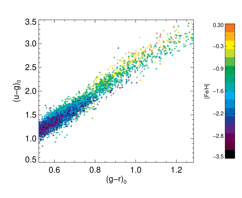
target types were specifically designed to detect K giants: these are designated “l-color K giants”, “red K giants”, and “proper-motion K giants”. The K-giant targets from these three categories all have , (shown as Firgue 1), and proper motions smaller than 11 mas/year. Figure 10 of Yanny et al. (2009) shows the
regions of the plane occupied by the three target types:
each category focuses on a particular region222Exact criteria
for each target type can be found at
https://www.sdss3.org/dr9/algorithms/segue_target_selection.php/#SEGUEts1. In
brief, the l-color K-giant category uses the metallicity sensitivity
of the color in the bluer part of the color range to preferentially select
metal-poor K giants. The two other categories focus on the redder
stars with : the red K-giant category selects those
stars whose luminosities place them above the locus of
foreground stars, while the proper-motion K-giant region is where
the K giants are found in the locus of foreground stars. In this location, only a
proper-motion selection can be used to cull the nearby dwarf
stars, because they have appreciable proper motions compared to the
distant giants.
We derived the sample of giants presented in this paper as follows. Using SDSS DR9 values in all cases, we start by requiring that the star has valid spectroscopic measurements of and log g from the SSPP. To eliminate main-sequence stars, we make a conservative cut on the SSPP estimate of log g by requiring . We restrict the star’s temperature by requiring that . Stars bluer than this color cutoff do not exhibit the luminosity-sensitive Mg/MgH feature with sufficient strength to use in the luminosity calibration; the red cutoff delineates the start of the M-star region. We further limit our sample by requiring that the reddening estimate from Schlegel et al. (1998) for each star, E(B-V), is less than 0.25 mag. We also apply additional data-quality criteria for both spectroscopy and photometry, as described in detail in Morrison et al. (in prep.). Most importantly, in addition to the SSPP log g measurement, we calculate a Mg index from the flux-corrected, but not continuum-corrected, SEGUE spectra. This index is a “pseudo equivalent width”, and identical to the Mg index described in Morrison et al. (2003), except for an adjustment to one of the continuum bands. We compare the value of this index at a given color with the index values for known globular and open cluster giants of different metallicity to decide whether a star is a giant or a dwarf, taking into account the SSPP value for the star. The index and its calibration using known globular cluster giants is described extensively in Morrison et al. (in prep.). It utilizes the strong luminosity sensitivity of the Mg Ib triplet and MgH features near 5200 333There is a similar index in the SSPP output, but this is based on continuum-corrected data. The continuum correction actually removes some of the signal from the strong MgH bands in K dwarfs, so this is not as sensitive as our index..
We need to keep track of the different targeting categories for our sample stars, as their metallicity distributions differ significantly. A complication is introduced by the fact that the SDSS photometry has been continually improved between the start of the SEGUE project in 2005 and Data Release in 2011. Because of the slight changes in and colors during this time, stars targeted using earlier photometry may not satisfy the criteria for target selection if one uses the most recent photometry. Note that we do not use kinematic selection criteria in our target selection, except for the proper-motion cut described above, which only affects giants with high velocity at very close distances (see Morrison et al. in prep., for more discussion.). This group includes stars targeted originally as K giants whose new photometry moved them out of the target boxes, and also stars targeted originally in other categories.
Using colors, reddening, log g values, and spectra from DR9, we find 15,750 field-star candidates that satisfy our K-giant criteria, have good photometry (i.e., color errors from SDSS pipeline are less than 0.04 mag), and have passed the Mg Ib triplet and MgH features criterion. We describe a further culling of the sample in §3.4, aimed at eliminating stars that could either be on the RGB or in the red clump. The error of for each K giant used in this paper is calibrated using cluster data plus repeat observations, which depends on the signal-to-noise ratio of the spectrum444The relation between the error of () and the signal-to-noise () ratio is expressed as for ; the out-of-range SN values are truncated to the nearest value of ., as described in detail in Morrison et al. (in prep.).
We show below that it is important to well-quantify the errors in color measurement. The two contributing factors here are the measurement errors on the color and on the reddening E(B-V). While the SDSS PHOTO pipeline gives estimates of measurement error on each color, these estimates do not include effects such as changes in sky transparency, mis-matches between the model used for the point spread function and the actual stellar image, and so on.
We estimate this additional factor as magnitudes in (Padmanabhan et al. 2008). To quantify the reddening errors, one of the authors (HLM) has selected 102 globular clusters from the compilation of Harris (1996, 2010 edition) with good color magnitude diagrams in the literature, and compared the estimates of E(B-V) from Schlegel et al. (1998, SFD hereafter) with those of Harris. Here we assume that the globular cluster reddenings represent “ground truth” for Galactic structure studies. We find that for objects with E(B-V) from SFD less than 0.25 mag (our limit for the K-giant investigation) there is a small offset (SFD reddenings are on average 0.01 mag higher than those of Harris). Assuming that both error estimates contribute equally to the differences between them, we find an error for the SFD reddenings of 0.013 mag.
Thus, to account for both of these effects, we add 0.017 magnitudes in quadrature to the estimate of error, and 0.037 magnitudes in quadrature to the estimate of the error from the SDSS pipeline.
3 Probabilistic Framework for Distance Estimates
Our goal is to obtain the posterior probability distribution function (pdf) for the distance modulus of any particular K-giant star, after accounting for (i.e., marginalizing over) the observational uncertainties in apparent magnitudes, colors, and metallicities (), and after including available prior information about the K-giant luminosity function, metallicity distribution, and, possibly, the halo radial density profile.
3.1 Distance Modulus Likelihoods
We start by recalling Bayes theorem, cast in terms of the situation at hand:
| (1) |
Here, is the pdf of the distance moduli, (), and describes the relative probability of different , in light of the data, {} (we use { } to denote the observational constraints, i.e., the estimates and the uncertainties for the observable quantities). is the likelihood of (e.g., ), and tells us how probable the data {} are if were true. The term is the prior probability for the , which reflects independent information about this quantity, e.g., that the stellar number density in the Galactic halo follows a power law of . The term is a non-zero constant.
So, the probability of the for a given star is proportional to the product of the likelihood of and the prior probability of (e.g., Eq 2).
| (2) |
The prior probability for the in Eq. 2 can be incorporated independently, and the main task is to derive . In deriving , we must in turn incorporate any prior information about other parameters that play a role, such as the giant-branch luminosity function, , or the metallicity distribution of halo giants, . This is done via:
| (3) |
Here we use FeH to denote the metallicity of the model, while we use for the observed metallicity of the star.
3.2 Observables and Priors
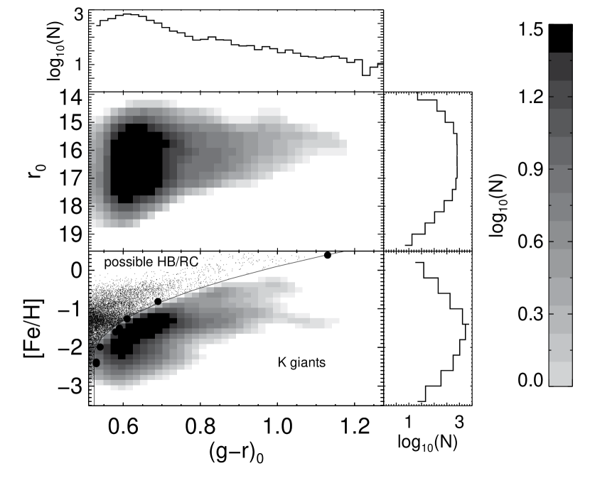
The direct observables we obtain from SEGUE and the SSPP are the extinction corrected apparent magnitudes, colors, metallicities, and their corresponding errors . Figure 1 shows the color-color diagram for our confirmed K giants, following application of the procedures described below. Figure 2 shows that the most common stars are the intrinsically fainter blue giants, as we would expect from the giant-branch luminosity function. Hereafter, we use and instead of and for convenience and generality in the expression of the formulas.
In our analysis, we can and should account for three pieces of prior (external) information or knowledge about the RGB population that go beyond the immediate measurement of the one object at hand: , and (shown as Eq. 1 and Eq. 3).
The prior probability of reflects any information on the radial density profile of the Milky Way’s stellar halo. Vivas & Zinn (2006) and Bell et al. (2008) indicated that the radial halo stellar density follows a power law , with the best value of , and reasonable values in the range ; this implies , . Quite fortuitously, the prior probability for turns out to be flat for the radial stellar density of a power law of . Given that the approximatively follows a Gaussian distribution with the mean of and standard deviation of (here is the error of ), the will shift the estimate of by , but with basically no change in . Therefore, the shifts in the mean caused by can be neglected for values of (i.e. ). In §3.6, we explicitly verify that different halo density profiles do not affect the distance estimation significantly using artificial data.
The prior probability of the absolute magnitude M can be inferred from the nearly universal luminosity function of the giant branch of old stellar populations. Specifically, we derive it from the globular clusters () and () (Sandquist et al. 1996, 1999), and from the Basti theoretical luminosity function with and (Pietrinferni et al. 2004). Figure 3 (top panel) shows that the luminosity functions for the RGBs derived from the globular clusters in the different bands are consistent with one another, and also with the Basti theoretic luminosity functions for the metal-rich and metal-poor cases. All the luminosity functions follow linear functions with similar slope, , as a result of the fact that the luminosity functions are insensitive to changes in the metallicity and color. According to and , the luminosity function means . We conclude that the luminosity function for the giant branch follows , shown as the dashed line in Figure 3.
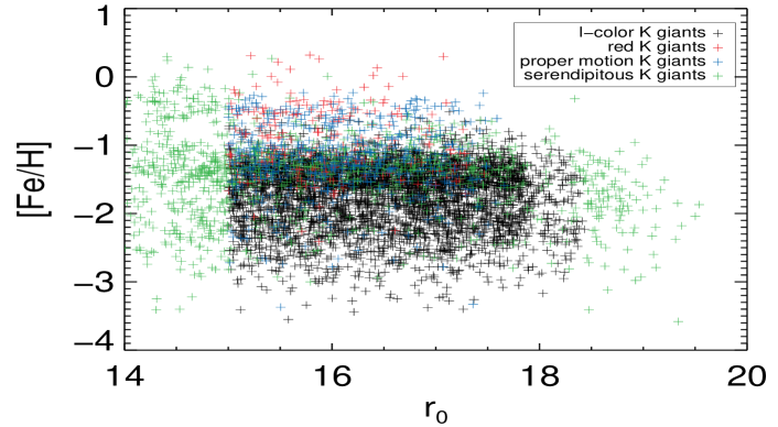
Our prior probability for results from an empirical approach. In the SEGUE target selection, the K giants were split into four sub-categories: the l-color K giants, the red K giants, the proper-motion K giants, and the serendipitous K giants. This suggests that one should adopt the overall metallicity distribution of each sub-category as the prior for any one star in this sub-category (Figure 4). Figure 4 shows the metallicity distribution variation with apparent magnitude in the upper panel, and the four priors in the lower panel. It can be seen that the four sub-categories have different metallicity distributions. For a star that has approximately the mean metallicity, this prior should leave unchanged, because the individual metallicity error is smaller than the spread of the . However, for a star of seemingly very low metallicity, the prior implies that this has been more likely an underestimated metallicity of a (intrinsically) less metal-poor star, which would lead to an overestimated distance modulus.
3.3 Color-Magnitude Fiducials
To obtain distance estimates, we determine an estimate of the absolute magnitude of each star, using its color and a set of giant-branch fiducials for clusters with metallicities ranging from to , and then use the star’s apparent magnitude (corrected for extinction using the estimates of Schlegel et al. 1998) to obtain its distance. We prefer to use fiducials, rather than model-isochrone giant branches wherever possible, because isochrone giant branches cannot reproduce cluster fiducials with sufficient accuracy.
As the SDSS imager saturates for stars brighter than , almost none of the clusters observed by SDSS and used by An et al. (2008) have unsaturated giant branches. Therefore, we derived such fiducials, using the globular clusters M92, M13, and M71, and the open cluster NGC6791, which have accurate photometry from the DAOphot reductions of An et al. (2008) for most of the stars; the giant branches can also be supplemented using the photometry of Clem et al. (2008). We transformed to using the transformations given in Tucker et al. (2006). Note that M71 is a disk globular cluster, and one of the few clusters in the North at this important intermediate metallicity. However, it has reddening that varies somewhat over the face of the cluster, making it a difficult cluster to work with. We use instead of to obtain more accurate estimates of the variable reddening map of M71, and use them to produce a better fiducial for this cluster (see Morrison et al. in prep. for details). We list our adopted values of , reddening, and distance modulus for each cluster in Table 1. In addition, we supplemented the fiducials with a Solar-metallicity giant branch from the Basti -enhanced isochrones (Pietrinferni et al. 2004). Figure 5 shows the four fiducials and the one theoretical isochrone. The color at a given and , , can then be interpolated from these color-magnitude fiducials.
It is important to note that most of the halo K giants are -enhanced, except for a few giants close to Solar metallicity (Morrison et al. in prep.). For less metal-poor K giants, the effect of on luminosity is stronger (for instance, the difference of r-band absolute magnitude can be as large as 0.5 mag at the tip of the giant branch for an -enhanced giant compared to one with Solar-scaled -element abundance but the same value). The cluster fiducials and one isochrone we use for distance estimates when are -enhanced, while above that metallicity, we assume gradual weakening of the -abundance, naturally introduced by the NGC6791 (Solar-scaled alpha abundances) fiducial line in the interpolation. In other word, when a giant’s is between Solar and the NGC6791 value, its -abundance is also assumed to be in between.
Given the sparse sampling of the M – space by the four isochrones, we need to construct interpolated fiducials. We do this by quadratic interpolation of , based on the three nearest fiducial points in color, and construct a dense color table for given and , which will be used for Eq. 4. Extrapolation beyond the metal-poor and metal-rich boundaries and the tip of the RGB would be poorly constrained. Therefore, we use these limiting fiducials instead for the rare cases of stars with or . Table 3 shows an interpolated fiducial with ; the entire catalog of 20 interpolated fiducials with metallicity ranging from to is provided in the electronic edition of the journal. While there is more than one way to interpolate the colors, such as quadratic or piecewise linear, we have checked and found that different interpolation schemes lead to an uncertainty less than mag in color, due to the sparsity of the fiducials, which could be an additional source of error in estimates.
3.4 Red Giant-Branch Stars vs. Red-Clump Giants
In addition, we have chosen not to assign distances to stars that lie on the giant branch below the level of the horizontal branch (HB). This is because the red horizontal-branch or red-clump (RC) giants in a cluster have the same color as these stars, but quite different absolute magnitudes, and the SSPP log g estimate is not sufficiently accurate to discriminate between the two options. We derive a relation between and the color of the giant branch at the level of the horizontal branch, using eight clusters with photometry from An et al. (2008), with cluster data given in Table 2. The and for the HB/RC of the clusters follow a quadratic polynomial, , as shown in Figure 2. We then use this polynomial and its estimate to work out, for each star, whether it is on the giant branch above the level of the HB. It turns out that more than half of the ucandidate K giants fall into the region of RGB - HB ambiguity.
To incorporate the errors of metallicities and colors, we envisage each star as a 2D (error-) Gaussian in the color-metallicity plane, centered on its most likely value and the 2D Gaussian having widths of color errors and metallicity errors, respectively. Then, we can calculate the “chance of being clearly RGB” as the fraction of the 2D integral over the 2D error-Gaussian that is to the right of the line.
Ultimately, we are left with 6036 stars with more than 45% chance of being clearly on the RGB, above the level of the HB. Of these, 5962 stars have more than 50% chance to be RGB, 5030 stars have more than 68% chance to be RGB, and 3638 stars have more than 90% chance to be RGB. In addition, 216 satisfy the target criteria for red K giants, 506 the criteria for proper-motion K giants, and 4246 the l-color K-giant criteria. Another 1068 were serendipitous identifications – stars targeted in other categories which nevertheless were giants. Figure 2 shows the distribution of the apparent magnitudes, , and metallicities, , along with the color, .
Besides the contamination from HB/RC stars, we need to consider possible contamination of our sample by asymptotic giant-branch (AGB) stars, because it is not possible for us to distinguish RGB from AGB stars with our spectra. While the difference in absolute magnitude can be large (reaching 0.8 mag, implying a 40% distance underestimate at the blue end of our giant color range), the proportion of our giants that are on the AGB is relatively small. We used both the luminosity function of Sandquist & Bolte (2004) for the globular cluster M5 and evolutionary tracks from Basti isochrones for old populations of metallicity and , to estimate the percentage of stars which are on the AGB. We find that for the most metal-poor stars, around 10% will be AGB stars, while for stars with close to the fraction is near 20%. For less metal-poor stars with , the expected fraction of AGB stars becomes larger than 20%, but in the SEGUE K-giant sample, less than 10% of stars have .
3.5 Implementation
For any given star, the observables are its apparent magnitude and associated error, , its color and error , and its metallicity and error . The and the data are linked through the absolute magnitude M via: and the fiducial , which we presume to be a relation of negligible scatter. Now we can incorporate the errors of the data and the specific priors on the stellar luminosity and metallicity distribution when calculating (see Eq. 3).
In practice, the errors on color, apparent magnitude, and metallicity can be approximated as Gaussian functions, in which case (see Eq. 3) is modeled as a product of Gaussian distributions with mean and Delta , , and :
| (4) |
For Eq. 3, we use the priors , based on the luminosity function of the giant branch, (Figure 3), and , based on the metallicity distributions of the K-giant sub-categories (Figure 4).
For any K giant with , we can then calculate by computing the integral of a bivariate function (Eq. 3) over dM and dFeH, using iterated Gaussian quadrature. As described in §3.2, the is taken as a constant for a halo density profile of , so . Then, the best estimate of is at the peak of , and its error is the central interval of (i.e. ).
To speed up the determination of the integral in Eq. 3, we look up in a pre-calculated and finely-sampled color table, instead of an actual interpolation. This approach can provide a consistent for given and , if the pre-prepared color table is suitable. We use a color table, , of size , with and .
3.6 Tests with Simulated Data Sets
To test whether our approach leads to largely unbiased estimates, a simulated data set was generated in order to mimic the SEGUE K-giant sample. As mentioned in §2, there are 4 sub-categories of K giants, and they have different distributions of , so the simulated stars were generated independently to mimic each sub-category. First, we produced a set of randomly-generated values of distance, luminosity, and , following a halo stellar density profile of , the luminosity function , and the metallicity distribution of each category of K giants, to cover similar ranges of as our sample of K giants. Then the apparent magnitudes and colors were calculated from and fiducials. Gaussian errors were added to directly observable quantities , with variances taken from observed SEGUE K giants with similar . Finally, a simulated star was accepted only if its magnitude and color fall within the selection criteria of the pertinent K-giant sub-category.
A total of 6036 simulated stars were generated according to the above procedure. The distributions in magnitude and in color are displayed in Figure 6, along with those of SEGUE K giants, showing that the simulated sample is a reasonable match, except for some apparent incompleteness at the faint end in the ’real’ data555We quote ‘real’ data to contrast with simulated data.. This sample was then analyzed using the same approach to estimate the that was applied to actually observed SEGUE K giants, using the known-to-be-correct priors. When considering the difference between the calculated distance modulus of each star and its true value, divided by the distance modulus uncertainty, , we should then expect a Gaussian of mean zero and a variance of unity. Indeed, we find a mean of and a variance of for the case of using luminosity and metallicity priors, but a mean of and a variance of for the case of neglecting the metallicity prior, and a mean of and a variance of for the case of neglecting the luminosity prior. Note that these are in units of , which is typically mag; therefore, any systematic biases in distance will be of order 1%. Using both priors should lead to unbiased distance estimates.
For the actual SEGUE data the priors are not known perfectly, as we do not know the overall density profile of the halo, particularly at large distances (Deason et al. 2011; Sesar et al. 2011). Previous work indicated that the halo radial stellar density follows a power law , with reasonable values of (Vivas & Zinn 2006; Bell et al. 2008). To test the influence of assuming a different , we made two sets of simulated data following or , according to the above procedure, and then applied the Bayesian approach to estimate by using a halo stellar density profile of , the luminosity function of , and the metallicity distribution of each category as priors. Considering the distribution of , we found a mean of and a dispersion of for the case and a mean of and a dispersion of for the case, very similar to the case, implying that the exact form of the prior for the halo density profile does not affect our results significantly. This is consistent with Burnett & Binney (2010), who also concluded that approximate priors in the analysis of a real sample will yield reliable results.
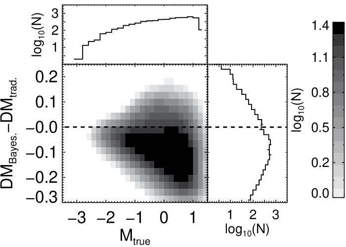
However, neglecting the luminosity and metallicity priors, as has often been done in previous work (Ratnatunga & Bahcall 1985; Norris et al. 1985; Beers et al. 2000), would lead to a mean systematic distance modulus bias of up 0.1 mag compared to neglecting both priors shown as Figure 7, which is also illustrated by the K-giant sample in Figure 11 and discussed in §4.2. Therefore, only an approach with explicit priors will lead to unbiased distance estimates.
4 Results
4.1 Distances for the SDSS/SEGUE K giants
The most immediate results of the analysis in §3.4 are estimates of the distance moduli and their uncertainties from (Figure 8). At the same time, we obtain estimates for the intrinsic luminosities by , distances from the Sun, and Galactocentric distances by assuming kpc. This results in the main entries in our public catalog for 6036 K giants: the best estimates of the distance moduli and their uncertainties (, ), heliocentric distances, and their errors (, ), Galactocentric distances and their errors (, ), the absolute magnitudes along with the errors (, ), and other parameters. In addition, we describe the by a set of percentages, which are also included in the on-line table. Table 4 shows an example of the online table of K giants. The complete version of this table is provided in the electronic edition of the journal.
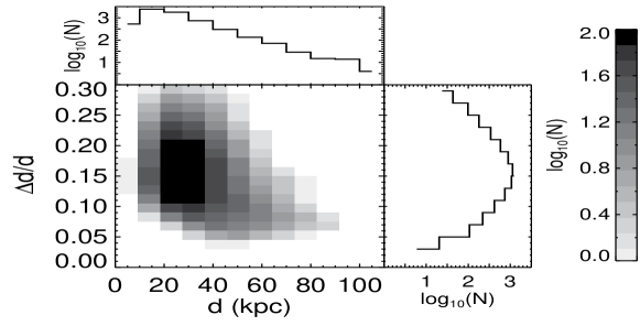
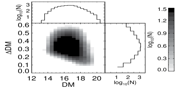
Figure 9 illustrates the overall properties of the ensemble of distance estimates. The top two panels show the mean precisions of in and mag in ; these panels also show that the fractional distances are less precise for more nearby stars, because they tend to be stars on the lower part of the giant branch, which is steep in the color-magnitude diagram, particularly at low metallicities.
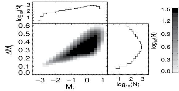
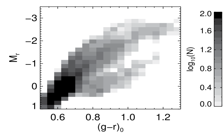
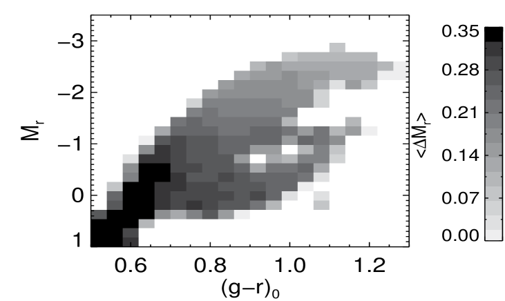
The bottom panel of Figure 9 shows that the mean error in is mag, and that faint giants have less precise intrinsic luminosity estimates. Figure 10 (upper panel) shows the distribution of K giants on the CMD. There are more stars in the lower part of the giant branch, which is consistent with the prediction of the luminosity function. The lower panel of Figure 10 shows that stars in the upper part of the RGB have more precise distances than those in the lower part of the CMD, because the fiducials are much steeper near the sub-giant branch. This is equivalent to the fact that the fractional distance precision is higher for the largest distances (see Figure 9).
The giants in our sample lie in the region of kpc from the Galactic center. There are 1647 stars beyond 30 kpc, 283 stars beyond 50 kpc, and 43 stars beyond 80 kpc (c.f., the red giants beyond kpc in Battaglia et al. 2005, halo stars beyond kpc in Deason et al. 2012 and no BHB stars beyond kpc in Xue et al. 2008, 2011). Our sample comprises the largest sample of distant stellar halo stars with measured radial velocities and distances to date.
4.2 The Impact of Priors
In this section we briefly analyze how important the priors actually were in deriving the distance estimates. For each star, the evaluation of Eq. 3 using Eq. 4 and the interpolated fiducials results in (Figure 8), i.e., the likelihood of the distance modulus, before folding in an explicit prior on , but after accounting for the priors on M and (Eq. 3). In this section we present some example , but first explore the systematic impact on of neglecting the and priors.
When estimating the distance to a given star, without the benefit of external prior information, one would evaluate Eq. 3 presuming that and are constant.
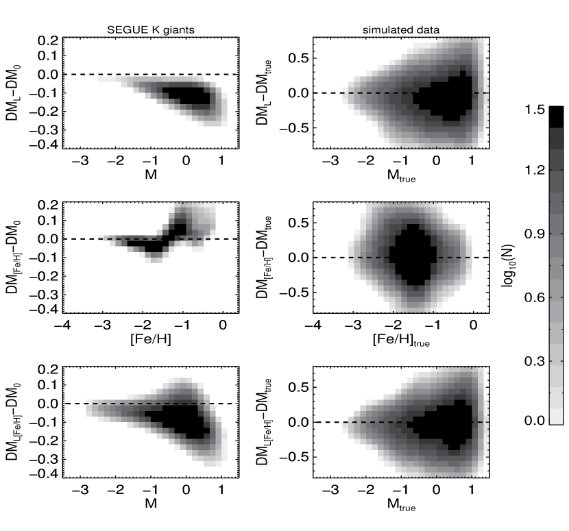
To test the impact of , we estimate the distances for two cases. No priors applied ( and ); and only the prior on the luminosity function applied ( and ). The distance modulus estimate that neglects the explicit priors is denoted as , while the distance modulus with only applied is marked as . The top of the left panel of Figure 11 illustrates the importance of including the ‘luminosity prior’, by showing the systematic difference in that results from neglecting it. For stars near the tip of the giant branch the bias is very small, but for stars near the bottom of the giant branch, the mean systematic bias of neglecting the luminosity prior information is mag, with systematic bias as high as mag in some cases.
To test the impact of , we estimate the distances where only the metallicity prior was applied, and mark the relevant as . Compared with the distance modulus with no priors applied, , we find can correct a mean overestimate of mag on the for the metal-poor stars and a mean underestimate of mag on the for the metal-rich ones, but the neglect of the metallicity prior causes a smaller bias in than neglecting the luminosity prior ( mag at mean), as shown in Figure 11 (middle of left panel). The distance modulus bias caused by neglecting both priors is presented in the bottom panel of Figure 11. Neglecting both priors causes a mean bias of mag and a maximum bias of mag in distance modulus.
4.3 Distance Precision Test using Clusters
We use five clusters (M13, M71, M92, NGC6791, and Berkeley29) to test the precision of the distance estimates, because they have spectroscopic members observed in SEGUE. Berkeley29 (Be29) is a comparatively young open cluster with age of 34 Gyr (Sestito et al. 2008), younger than our adopted fiducials (1012 Gyr). It illustrates how distances could be in error as a result of an incorrect age prior. M71 is a disk globular cluster. Because of its low Galactic latitude (less than 5 degrees from the disk plane) and relatively circular orbit, separation of genuine M71 members from field stars is much more difficult than for halo clusters (M13 and M92). The analysis concerning the membership of stars in the stellar clusters will be reported in detail in the Appendix of the Morrison et al. (in prep.).
In general, we identify cluster membership using proper motion and radial velocity. The proper motions provide a membership probability for each star(Cudworth 1976; Cudworth & Monet 1979; Cudworth 1985; Rees 1992), and then the radial velocities are used for further membership checks, as described in detail in Morrison et al. (in preparation).
Based on the color-magnitude diagram (CMD) of the clusters, we select giant members with and above the sub-giant branch of the clusters to test the distance precision. The range of signal-to-noise ratio for the spectra of the cluster giant stars is , and the SN rang for K-giant spectra is . Here we do not apply the very stringent criterion to eliminate HB/RC stars described in §3.4, because this criterion also culls many lower RGB stars that are useful for the test. Figure 12 shows there are some HB/RC stars or AGB stars, which can help verify how distances would be in error for the non-RGB stars. Furthermore, we do not use the members with dex, because of the strong sensitivity of the distances to metallicity errors.
We estimate the for each selected member RGB star, adopting the luminosity prior of , and a Dirac delta function centered at the literature cluster metallicity, , as the metallicity prior. Figure 13 shows the difference between our individual estimate for each selected member RGB star and the literature (shown in Table 1) for M13, M71, M92 and NGC6791 respectively. Since M71 has significant differential reddening and fewer members, it is not a suitable cluster to verify the distance errors to little-reddened, usually more metal-poor halo giants. However, all 4 M71 members exhibit less than mag scatter from , as shown in Figure 13. The RGB members show consistent distances with the literature value derived by main-sequence fitting within 1, but the distance moduli are underestimated by a maximum mag for the non-RGB stars. Fortunately, the criterion to eliminate HB/RC stars adopted in §3.4 is sufficiently stringent to cull all HB/RC stars and many lower-RGB stars. As mentioned previously, there is a relative paucity of AGB stars in the SEGUE K-giant sample.
The mean values of for the RGB members at different color ranges are within mag. Compared to the typical error of mag in , our estimates of are reasonably precise.
Figure 14 shows the distributions of Be29 members around their fiducials. Be29 members are far from the interpolated fiducial based on our old fiducials. The old fiducials lead to totally wrong distance estimates for relatively young giants in Be29, as shown in Figure 15. If the age prior is wrong, the distance estimates are unreliable. The derived errors on the distance moduli of the K giants are only valid if the ages of the K giants are older than 10 Gyr.
In addition, we calculate the distances with flat priors (which means no priors), and find that neglecting the priors would lead to biases in distance of from the literature values for NGC6791, M71, M13 and M92. However, we only find biases in distance of the literature values for NGC6791, M71, M13 and M92 when using both priors. Therefore, neglecting the priors would lead to biased distance estimates.
5 Summary and Conclusions
We have implemented a probabilistic approach to estimate the distances for SEGUE K giants in the Galactic halo. This approach folds all available observational information into the calculation, and incorporates external information through priors, resulting in a likelihood for each star that provides both a distance estimate and its uncertainty.
The priors adopted in this work are the giant-branch luminosity function derived from globular clusters, and the ensemble metallicity distributions for different SEGUE K-giant target categories. We show that these priors are needed to prevent systematic overestimate of the distance moduli by up to mag. The role of the priors are important, and make the results more reliable.
We employed empirical color-magnitude fiducials from old stellar clusters to obtain the predicted colors , which are needed to calculate . Ultimately, the best estimates of the distance moduli and their errors can be estimated using the peak and central interval of .
We used a simulated data set to verify that our distance estimates are close to optimal and are nearly unbiased: any systematic biases in distance will be of order 1%. We verified that the exact form of the prior for the halo density profile does not affect our results significantly, which is consistent with the conclusion of Burnett & Binney (2010). Neglecting the luminosity and metallicity priors, as has often been done in previous distance analyses, will lead to a mean systematic bias in distance modulus of mag, which shows the advantage of our Bayesian method.
With this approach we obtain the distance moduli, and thus, absolute magnitudes and distances, for K giants that have a mean distance precision of , or mag in and . The sample contains stars beyond kpc, which makes it by far the largest sample of distant stellar halo stars with measured radial velocities and distances to date.
We tested the accuracy of our distance estimates using RGB member stars in the clusters M13, M92, M71, NGC6791 and Be29, which have SEGUE spectroscopic observations. We found that the distance estimates for the individual cluster member RGB star derived with Bayesian approach are consistent with the literature distance moduli of the clusters within 1. In addition, we found our fiducials would lead to substantially incorrect distance estimates for young giants ( Gyrs), based on our test for Be29.
We present an online catalog containing the distance moduli, observed information and SSPP atmospheric parameters for the 6036 SEGUE K giants. For each object in the catalog we also list some of the basic observables such as (RA, Dec), extinction-corrected apparent magnitudes and de-reddened colors, as well as the information obtained from the spectra– heliocentric radial velocities plus SSPP atmospheric parameters. In addition, we provide the Bayesian estimates of the distance moduli, distances to the Sun, Galactocentric distances, the absolute magnitudes and their uncertainties, along with the distance moduli at confidence of .
We caution the reader that the [Fe/H] cannot be used to obtain the halo profile and the metallicity distribution directly, because the complex SEGUE selection function needs to be taken into account.
References
- Ahn et al. (2012) Ahn, C. P., Alexandroff, R., Allende Prieto, C., et al. 2012, ApJS, 203, 21
- Allende Prieto et al. (2008) Allende Prieto, C., Sivarani, T., Beers, T. C., et al. 2008, AJ, 136, 2070
- An et al. (2008) An, D., Johnson, J. A., Clem, J. L., et al. 2008, ApJS, 179, 326
- Battaglia (2007) Battaglia, G. 2007, PhD thesis, Kapteyn Astronomical Institute, University of Groningen
- Battaglia et al. (2005) Battaglia, G., Helmi, A., Morrison, H., et al. 2005, MNRAS, 364, 433
- Beers et al. (2000) Beers, T. C., Chiba, M., Yoshii, Y., et al. 2000, AJ, 119, 2866
- Bell et al. (2008) Bell, E. F., Zucker, D. B., Belokurov, V., et al. 2008, ApJ, 680, 295
- Bond (1980) Bond, H. E. 1980, ApJS, 44, 517
- Brogaard et al. (2011) Brogaard, K., Bruntt, H., Grundahl, F., et al. 2011, A&A, 525, A2
- Burnett & Binney (2010) Burnett, B. & Binney, J. 2010, MNRAS, 407, 339
- Burnett et al. (2011) Burnett, B., Binney, J., Sharma, S., et al. 2011, A&A, 532, A113
- Carraro et al. (2004) Carraro, G., Bresolin, F., Villanova, S., et al. 2004, AJ, 128, 1676
- Carraro et al. (2006) Carraro, G., Villanova, S., Demarque, P., et al. 2006, ApJ, 643, 1151
- Carretta et al. (2000) Carretta, E., Gratton, R. G., Clementini, G., & Fusi Pecci, F. 2000, ApJ, 533, 215
- Clem et al. (2008) Clem, J. L., Vanden Berg, D. A., & Stetson, P. B. 2008, AJ, 135, 682
- Cudworth (1976) Cudworth, K. M. 1976, AJ, 81, 975
- Cudworth (1985) Cudworth, K. M. 1985, AJ, 90, 65
- Cudworth & Monet (1979) Cudworth, K. M. & Monet, D. G. 1979, AJ, 84, 774
- Deason et al. (2011) Deason, A. J., Belokurov, V., & Evans, N. W. 2011, MNRAS, 416, 2903
- Deason et al. (2012) Deason, A. J., Belokurov, V., Evans, N. W., et al. 2012, MNRAS, 425, 2840
- Eisenstein et al. (2011) Eisenstein, D. J., Weinberg, D. H., Agol, E., et al. 2011, AJ, 142, 72
- Fukugita et al. (1996) Fukugita, M., Ichikawa, T., Gunn, J. E., et al. 1996, AJ, 111, 1748
- Gratton et al. (2006) Gratton, R., Bragaglia, A., Carretta, E., & Tosi, M. 2006, ApJ, 642, 462
- Grundahl et al. (2002) Grundahl, F., Stetson, P. B., & Andersen, M. I. 2002, A&A, 395, 481
- Gunn et al. (1998) Gunn, J. E., Carr, M., Rockosi, C., et al. 1998, AJ, 116, 3040
- Gunn et al. (2006) Gunn, J. E., Siegmund, W. A., Mannery, E. J., et al. 2006, AJ, 131, 2332
- Harris (1996) Harris, W. E. 1996, AJ, 112, 1487
- Kraft & Ivans (2003) Kraft, R. P. & Ivans, I. I. 2003, PASP, 115, 143
- Lee et al. (2011) Lee, Y. S., Beers, T. C., Allende Prieto, C., et al. 2011, AJ, 141, 90
- Lee et al. (2008a) Lee, Y. S., Beers, T. C., Sivarani, T., et al. 2008a, AJ, 136, 2022
- Lee et al. (2008b) Lee, Y. S., Beers, T. C., Sivarani, T., et al. 2008b, AJ, 136, 2050
- Morrison et al. (1990) Morrison, H. L., Flynn, C., & Freeman, K. C. 1990, AJ, 100, 1191
- Morrison et al. (2000) Morrison, H. L., Mateo, M., Olszewski, E. W., et al. 2000, AJ, 119, 2254
- Morrison et al. (2003) Morrison, H. L., Norris, J., Mateo, M., et al. 2003, AJ, 125, 2502
- Norris et al. (1985) Norris, J., Bessell, M. S., & Pickles, A. J. 1985, ApJS, 58, 463
- Padmanabhan et al. (2008) Padmanabhan, N., Schlegel, D. J., Finkbeiner, D. P., et al. 2008, ApJ, 674, 1217
- Perryman et al. (1997) Perryman, M. A. C., Lindegren, L., Kovalevsky, J., et al. 1997, A&A, 323, L49
- Peterson & Green (1998) Peterson, R. C. & Green, E. M. 1998, ApJ, 502, L39
- Pier et al. (2003) Pier, J. R., Munn, J. A., Hindsley, R. B., et al. 2003, AJ, 125, 1559
- Pietrinferni et al. (2004) Pietrinferni, A., Cassisi, S., Salaris, M., & Castelli, F. 2004, ApJ, 612, 168
- Ratnatunga & Bahcall (1985) Ratnatunga, K. U. & Bahcall, J. N. 1985, ApJS, 59, 63
- Rees (1992) Rees, Jr., R. F. 1992, AJ, 103, 1573
- Sandquist & Bolte (2004) Sandquist, E. L. & Bolte, M. 2004, ApJ, 611, 323
- Sandquist et al. (1999) Sandquist, E. L., Bolte, M., Langer, G. E., Hesser, J. E., & Mendes de Oliveira, C. 1999, ApJ, 518, 262
- Sandquist et al. (1996) Sandquist, E. L., Bolte, M., Stetson, P. B., & Hesser, J. E. 1996, ApJ, 470, 910
- Schlegel et al. (1998) Schlegel, D. J., Finkbeiner, D. P., & Davis, M. 1998, ApJ, 500, 525
- Sesar et al. (2011) Sesar, B., Jurić, M., & Ivezić, Ž. 2011, ApJ, 731, 4
- Sestito et al. (2008) Sestito, P., Bragaglia, A., Randich, S., et al. 2008, A&A, 488, 943
- Smee et al. (2013) Smee, S. A., Gunn, J. E., Uomoto, A., et al. 2013, AJ, 146, 32
- Smolinski et al. (2011) Smolinski, J. P., Lee, Y. S., Beers, T. C., et al. 2011, AJ, 141, 89
- Starkenburg et al. (2009) Starkenburg, E., Helmi, A., Morrison, H. L., et al. 2009, ApJ, 698, 567
- Stoughton et al. (2002) Stoughton, C., Lupton, R. H., Bernardi, M., et al. 2002, AJ, 123, 485
- Tucker et al. (2006) Tucker, D. L., Kent, S., Richmond, M. W., et al. 2006, Astronomische Nachrichten, 327, 821
- Vivas & Zinn (2006) Vivas, A. K. & Zinn, R. 2006, AJ, 132, 714
- Xue et al. (2011) Xue, X.-X., Rix, H.-W., Yanny, B., et al. 2011, ApJ, 738, 79
- Xue et al. (2008) Xue, X. X., Rix, H. W., Zhao, G., et al. 2008, ApJ, 684, 1143 [X08]
- Yanny et al. (2009) Yanny, B., Rockosi, C., Newberg, H. J., et al. 2009, AJ, 137, 4377
- York et al. (2000) York, D. G., Adelman, J., Anderson, Jr., J. E., et al. 2000, AJ, 120, 1579






| NGC | Messier | E(B-V) | ||
|---|---|---|---|---|
| 6341 | M92 | 0.02aaKraft & Ivans (2003); their globular cluster metallicity scale is based on the Fe lines from high-resolution spectra of giants. | 14.64bbCarretta et al. (2000); derived from the Hipparcos sub-dwarf fitting. | –2.38aaKraft & Ivans (2003); their globular cluster metallicity scale is based on the Fe lines from high-resolution spectra of giants. |
| 6205 | M13 | 0.02aaKraft & Ivans (2003); their globular cluster metallicity scale is based on the Fe lines from high-resolution spectra of giants. | 14.38bbCarretta et al. (2000); derived from the Hipparcos sub-dwarf fitting. | –1.60aaKraft & Ivans (2003); their globular cluster metallicity scale is based on the Fe lines from high-resolution spectra of giants. |
| 6838 | M71 | 0.28ccGrundahl et al. (2002); derived from the Hipparcos (Perryman et al. 1997) sub-dwarf fitting. | 12.86ccGrundahl et al. (2002); derived from the Hipparcos (Perryman et al. 1997) sub-dwarf fitting. | –0.81aaKraft & Ivans (2003); their globular cluster metallicity scale is based on the Fe lines from high-resolution spectra of giants. |
| 6791 | 0.16ddBrogaard et al. (2011); is based on assuming . | 13.01ddBrogaard et al. (2011); is based on assuming . | +0.39eesimple average of the +0.29, +0.47, +0.4 and +0.39 by Brogaard et al. (2011), Gratton et al. (2006), Peterson & Green (1998), and Carraro et al. (2006) respectively. | |
| Be29ffreddening is from Carraro et al. (2004), is from Sestito et al. (2008) and is the average of the values from Carraro et al. (2004) and Sestito et al. (2008). | 0.08 | 15.6 | –0.38 |
- •
| NGC6791 | +0.39 | 1.13 |
|---|---|---|
| M71 | –0.81 | 0.69 |
| M5 | –1.26 | 0.61 |
| M3 | –1.50 | 0.59 |
| M13 | –1.60 | 0.58 |
| M53 | –1.99 | 0.54 |
| M92 | –2.38 | 0.53 |
| M15 | –2.42 | 0.53 |
-
•
The first column lists the names of the clusters; the next two columns provide the of the clusters and the extinction corrected color .
| 0.473 | 3.000 |
|---|---|
| 0.491 | 2.546 |
| 0.527 | 1.747 |
| 0.545 | 1.470 |
| 0.581 | 0.985 |
| 0.599 | 0.790 |
| 0.635 | 0.429 |
| 0.671 | 0.087 |
| 0.706 | -0.237 |
| 0.742 | -0.523 |
| 0.778 | -0.782 |
| 0.814 | -1.013 |
| 0.850 | -1.225 |
| 0.886 | -1.422 |
| 0.921 | -1.596 |
| 0.957 | -1.746 |
| 0.993 | -1.888 |
| 1.029 | -2.010 |
| 1.065 | -2.116 |
| 1.101 | -2.227 |
| 1.136 | -2.321 |
| 1.172 | -2.403 |
| 1.208 | -2.477 |
| 1.244 | -2.545 |
| 1.280 | -2.609 |
| 1.316 | -2.668 |
| 1.351 | -2.725 |
-
•
An example of one interpolated fiducial with =–1.18. The entire catalog of 50 interpolated fiducials with metallicity ranging from to is provided in the electronic edition of the journal.
| (km) | (km) | (K) | ||||||||||
| 154.7659 | -0.8354 | 17.257 | 0.040 | 0.965 | 0.028 | 43.7 | 2.5 | 4626 | -0.71 | 0.16 | 3.28 | 18.13 |
| 174.6570 | -0.9330 | 17.036 | 0.041 | 0.590 | 0.035 | 147.0 | 3.6 | 5259 | -1.50 | 0.15 | 2.59 | 16.37 |
| 189.9634 | 1.0202 | 17.078 | 0.040 | 0.558 | 0.028 | 122.7 | 6.1 | 5296 | -1.89 | 0.19 | 2.99 | 16.41 |
| 196.0723 | -0.5404 | 16.891 | 0.041 | 0.526 | 0.030 | -169.5 | 4.2 | 5158 | -2.12 | 0.15 | 1.75 | 16.03 |
| 205.9106 | -0.3442 | 18.067 | 0.041 | 0.631 | 0.031 | 86.5 | 4.5 | 4901 | -1.23 | 0.21 | 1.98 | 17.68 |
| (mag) | (mag) | (kpc) | (kpc) | |||||||||
| 17.62 | 17.85 | 18.21 | 18.62 | 18.83 | 0.38 | -0.88 | 0.39 | 42.35 | 7.89 | 45.51 | 7.78 | 1.00 |
| 15.43 | 15.81 | 16.33 | 16.79 | 17.07 | 0.49 | 0.67 | 0.49 | 18.78 | 4.11 | 20.55 | 3.79 | 0.67 |
| 15.56 | 15.90 | 16.39 | 16.86 | 17.14 | 0.48 | 0.66 | 0.48 | 19.17 | 4.18 | 19.27 | 3.82 | 0.75 |
| 15.00 | 15.40 | 15.96 | 16.46 | 16.76 | 0.53 | 0.86 | 0.53 | 16.05 | 3.79 | 15.64 | 3.31 | 0.51 |
| 17.00 | 17.29 | 17.68 | 18.07 | 18.32 | 0.39 | 0.39 | 0.39 | 34.38 | 6.24 | 31.74 | 6.07 | 0.66 |
-
•
The first two columns list the position (RA, Dec) for each object. The magnitudes,colors, and their errors are provided in the next four columns: corrected for extinction. The heliocentric radial velocities and their errors are listed in the next two columns. The next four columns contain the stellar atmospheric parameters and the errors in the metallicities as a relation of signal-to-noise ratio. Effective temperatures and surface gravities are not used in our work, and they are all published in SDSS DR9, so we recommend interested readers download their errors from CasJob. The at the peak and confidence of are listed in the next six columns. is the best estimate of the distance modulus for the K giant. The is the uncertainty of the distance modulus, which is calculated from . The last seven columns are absolute magnitude and distances calculated from , assuming kpc (i.e., , ), and the chance of being clearly RGB. The complete version of this table is provided in the electronic edition of the journal. The printed edition contains only a sample.