Degeneracy between mass and spin in black-hole-binary waveforms
Abstract
We explore the degeneracy between mass and spin in gravitational waveforms emitted by black-hole binary coalescences. We focus on spin-aligned waveforms and obtain our results using phenomenological models that were tuned to numerical-relativity simulations. A degeneracy is known for low-mass binaries (particularly neutron-star binaries), where gravitational-wave detectors are sensitive to only the inspiral phase, and the waveform can be modelled by post-Newtonian theory. Here, we consider black-hole binaries, where detectors will also be sensitive to the merger and ringdown, and demonstrate that the degeneracy persists across a broad mass range. At low masses, the degeneracy is between mass ratio and total spin, with chirp mass accurately determined. At higher masses, the degeneracy persists but is not so clearly characterised by constant chirp mass as the merger and ringdown become more significant. We consider the importance of this degeneracy both for performing searches (including searches where only non-spinning templates are used) and in parameter extraction from observed systems. We compare observational capabilities between the early (2015) and final (2018 onwards) versions of the Advanced LIGO detector.
I Introduction
The advanced LIGO and Virgo detectors are likely to allow us to observe numerous black-hole-binary coalescences in the coming years Abadie et al. (2010); Dominik et al. (2012). While the detectors are being installed, the challenge is to devise search and source extraction methods that will identify all black-hole-binary signals in the data whilst also allowing for the most accurate estimation of the source parameters possible.
Our understanding of gravitational waveforms emitted by black-hole mergers has improved dramatcially over the past five years, with the aid of a large number of numerical simulations, from which several models of the waveforms have been constructed (see e.g., Ref Ohme (2012) for an overview). A large fraction of the simulations have focussed on non-precessing systems (where the black holes are either non-spinning or have spins aligned with the orbital angular momentum); see, for example, Refs. Hannam (2009) and Ajith et al. (2012). Other than for high black-hole spins (greater than ), this space has been rather well covered for comparable-mass binaries, and several waveform models are available Ajith et al. (2011); Santamaria et al. (2010); Pan et al. (2010). The models characterize waveforms based on the masses of the two components and, in the case of the models we will consider in this paper, the total spin of the system. We will make use of these waveform models to investigate degeneracies in the waveforms. Since we are only considering a three-dimensional subspace of the full eight-dimensional space of binary masses and spins, many effects, most notably precession, cannot be probed. However, it is interesting to consider this smaller space because it is very likely that any degeneracies will persist in the full parameter space. Furthermore, recent results have shown that the waveform for a precessing binary can be factorized into precessional effects and a non-precessional part that is well modelled by the three parameters we consider here Schmidt et al. (2012).
In post-Newtonian (PN) theory, there is a well known degeneracy between the black holes’ mass ratio and the total spin, which arises at 1.5PN order, while a combination of the total mass and mass ratio (the “chirp mass”) remains relatively well constrained Cutler and Flanagan (1994a); Poisson and Will (1995). Here, our focus is on higher-mass waveforms that include a merger and ringdown. We demonstrate that the degeneracy persists in the full waveforms and also up to higher masses where only the later part of the inspiral and the merger/ringdown are in the detector’s sensitivity band. However, for the high-mass binaries, the degeneracy in mass and spin is not so clearly characterized by the chirp mass.
A degeneracy in the emitted gravitational waveform across the parameter space has numerous consequences for gravitational wave (GW) searches, both good and bad. The positive effect is that a degeneracy in the parameter space will reduce the volume that needs to be searched, thereby reducing the computational cost and trials factor associated with the search. The majority of searches of LIGO and Virgo data have made use of non-spinning components in the template waveforms (see e.g., Refs. Abadie et al. (2012, 2011)). A degeneracy between mass and spin means that the template waveforms have covered a larger fraction of the parameter space than might be naively expected. Furthermore, it has recently been argued that a two-dimensional bank of templates is sufficient to cover the space of spinning neutron-star binaries Brown et al. (2012). In this paper, we investigate the effect of using non-spinning waveforms in a search for black-hole binaries with spins and show that the mass-spin degeneracy renders the search more sensitive to spinning systems than might be expected. Nevertheless, a search using waveforms incorporating spin effects would be a significant improvement and the degeneracy should make it computationally feasible.
On the other hand, a degeneracy has a negative effect on parameter estimation. To make the most of gravitational-wave observations, accurate extraction of the physical parameters is of paramount importance. There are detailed multi-dimensional methods under development to accurately recover the parameters van der Sluys et al. (2008a, b); Veitch and Vecchio (2010); Feroz et al. (2009). However, there’s nothing that can be done about a real degeneracy in the emitted waveforms — there is no way of telling them apart. We evaluate the effects of mass-spin waveform degeneracy on our ability to accurately recover masses and spins and discuss the astrophysical implications. In the process we introduce a simple method to estimate the parameter-estimation confidence intervals.
Throughout the paper, we will provide sample results using a number of waveforms at different masses and mass ratios. We also make use of a number of noise curves for the advanced detectors, to illustrate how this effect is likely to change as the detectors approach their final, design sensitivity. No attempt has been made to perform an exhaustive study across the full parameter space, and this is left as a future project.
The layout of the paper is as follows: in Sec. II we outline the waveform models that we use, and discuss some of the assumptions that went into producing them and their range of applicability. We also discuss the interpretation of results in terms of mismatches between waveforms and introduce the detector noise curves used in our studies. In Sec. III we focus on the degeneracy between mass ratio and spin for low-mass binaries, giving the post-Newtonian argument for this degeneracy and illustrating the degeneracy for a number of cases and different detector sensitivities, and discuss implications for searches. Then, in Sec. IV we extend the results to higher mass binaries and show that the degeneracy persists, although in a different form. In Sec. V we discuss implications for the accurate estimation of parameters and astrophysical inference.
II Model and methods
II.1 The phenomenological waveform models
We describe the GW signal from black-hole binaries with non-precessing spins (i.e., the spins are aligned or anti-aligned with the binary’s orbital angular momentum) using the phenomenological models presented in Refs. Ajith et al. (2011) and Santamaria et al. (2010). For consistency with the labelling used within the LIGO-Virgo Collaboration LAL we refer to these models respectively as “PhenomB” and “PhenomC”. (“PhenomA” refers to an earlier model of non-spinning binaries Ajith et al. (2007a, 2008); Ajith (2008).) In both models the waveforms are parametrized by their total mass , mass ratio , and an effective total spin parameter,
| (1) | |||||
where for each black hole with angular momentum , , and the symmetric and anti-symmetric combinations of the spins are and . The phenomenological models incorporate a PN description of the inspiral, while the merger and ringdown regimes are tuned using the results of numerical simulations.
Both models have the same basic structure. The waveform is represented in the Fourier domain as . The amplitude and phase are modelled separately, using input from PN theory (inspiral), the observed properties of NR waveforms (plunge-merger), or results from perturbation theory (ringdown). The models are all power series in the frequency , and the coefficients in the model are written as polynomials in the two physical parameters and (the total mass is an overall scale factor), and it is the coefficients of these polynomials that are then calibrated to hybrids of PN and NR waveforms. For both models, the amplitude is constructed in a similar manner, with expressions for each of the inspiral, plunge-merger, and ringdown portions of the waveform modelled independently. In PhenomB Ajith et al. (2011) the three parts are connected as piecewise functions, and in PhenomC Santamaria et al. (2010) smooth -function interpolation is used. To obtain an expression for the phasing, PhenomB uses a single series expansion, matching the coefficients beyond leading order to hybrid waveforms, as well as results from the test mass () limit. PhenomC, on the other hand, uses the complete TaylorF2 PN inspiral phasing, and only the late inspiral/merger phase is fitted in a narrow frequency range to numerical simulations, while the ringdown waveform is obtained from analytically derived quasi-normal mode expressions for the frequency and attached continuously to the merger phase. There are 54 free parameters in PhenomB, and 45 in PhenomC, although the final models are both functions of only . There are three notable differences between the two models: (1) the PhenomB PN-NR hybrids are produced in the time domain, using TaylorT1 for the PN part, and the PhenomC hybrids are produced in the frequency domain, using TaylorF2 for the PN part Ajith et al. (2007b); (2) PhenomB incorporates information about the test-mass limit; (3) in PhenomC the phase evolution during inspiral incorporates PN calculations up to 3.5PN order (although the spin terms are complete only up to 2.5PN), while in PhenomB only the leading-order PN inspiral term is fixed, and the remaining terms up to 3.5PN order are tuned to the hybrid waveforms.
There is good qualitative agreement between the two models Santamaria et al. (2010), although no detailed quantitative comparison has yet been performed. We choose to work with PhenomB for generating the results presented in this paper. We have also cross-checked some of the calculations against PhenomC, and we comment further on this in Sec. IV.
II.2 Detectors and noise curves
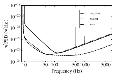
In this paper we compare spinning- and non-spinning-binary signals with reference to the expected sensitivity of the Advanced LIGO detector (aLIGO) Abbott et al. (2009); Shoemaker (2009); Harry and the LIGO Scientific Collaboration (2010). The sensitivity curves we use are shown in Fig. 1. During the early science runs, expected around 2015, the advanced LIGO detector is unlikely to be at its full design sensitivity. Consequently, we use the “early aLIGO” noise curve Shoemaker, David and Losurdo, Giovanni (2010) to give results indicative of what may be achieved in the early runs. At its optimum sensitivity several years later, the anticipated sensitivity is given by the “zero-detuned high-power” noise curve The LIGO Scientific Collaboration (2009). In this paper we will take that as the “final” design sensitivity of the detector. Over the parameter space of binaries that we study in this paper, the early aLIGO curve represents a sensitivity of roughly five times greater in the signal-to-noise ratio (SNR) than in the initial LIGO detectors during their final S6 science run, which corresponds to an increase in potential sources of two orders of magnitude. The final curve represents a further factor of three improvement in SNR, or about 30 times as many potential sources over early aLIGO. Finally, we also consider the “no signal recycling” (no-SRM) configuration of the detector, that could be achieved by the aLIGO detector operating without a signal recycling cavity. This has comparable low-frequency sensitivity to the final configuration, but significantly worse sensitivity at high frequencies. Although it is unlikely to be an observational mode, the non-signal-recycled curve offers a means to compare the effects of low and high frequency sensitivity upon our results.
II.3 Waveform Mismatches
We use the standard inner product between two waveforms, and with respect to the power spectral density of a detector Cutler and Flanagan (1994b),
| (2) |
The match between two waveforms is defined as their normalized inner product, maximized over time and phase shifts of the waveform,
| (3) |
Alternatively, we can consider the situation of a true waveform produced by a physical source, , and a model waveform that we will use to search for the real signal in detector data. If we normalize both waveforms, then we can split the model waveform into a component parallel to the true waveform, plus a component that is orthogonal to the true waveform, in the sense of our inner product. In other words, we have
| (4) |
where is the normalized “error” waveform that satisfies . In this form, the match is . Thus, the match is directly related to the (relative) amplitude of the “error” waveform.
In a GW search, a template bank of model waveforms is constructed Babak et al. (2006) such that the match between every point in the waveform parameter space and the nearest template in the bank is at least 0.97. Assuming that the model waveforms are physically correct, such a template bank ensures that we will lose no more than 10% of signals in our search. (A match of 0.97 means that the sensitivity range of the detector is only 97% of its optimum, and the detector is therefore sensitive to only of its optimum volume, and so we lose about 10% of signals.)
If the physical waveforms do not agree exactly with the model waveforms, this will lead to an additional loss in match between a signal and the best matched template, and consequently a reduction in the number of signals observed above threshold. In addition, to counter non-stationary detector noise, a number of signal consistency tests are included into analyses to distinguish signals from non-stationarities or “glitches” in the data Babak et al. (2012). These tests are used to either remove completely any transients that do not match the templates or else to down-weight their significance. Since searches performed to date have made use of non-spinning waveform families these thresholds have been set relatively loosely (and tested with spinning signals) to ensure they are not removing signals. For the high matches between signal and template we consider in this paper, the effect of signal consistency tests will be minimal, and we will not consider it further.
In the next sections we will identify the regions of the non-spinning waveform parameter space that provide a match of greater than 0.97 with the chosen waveform (which will usually incorporate spin). In doing so, we densely sample the non-spinning waveforms to identify all points with a match above 0.97. When performing a search, there will then be two contributions to the mismatch between the signal and the best matched template: one due to the difference between the waveform and search space and a second arising from the discrete sampling of the template space. The match between the signal and the closest template is guaranteed to be above 0.94 as the mismatches add linearly in this case (see e.g. Lindblom et al. (2008) for details). We are therefore requiring that the potential loss of SNR due to a mismatch between the model waveform and true waveform is no greater than the maximum possible loss due to the discreteness of the template bank.
We will also investigate how the parameters of the best-match non-spinning waveform vary when the signal corresponds to a non-precessing binary. In Sec. V we will see how the match can be used to give an estimate of the parameter estimation accuracy.
III Degeneracy between and at low masses
We first consider the degeneracy between the symmetric mass ratio and the effective total spin of the binary. This effect is already well known in PN theory Cutler and Flanagan (1994a); Poisson and Will (1995), which we will discuss first, and then we will look at inspiral-merger-ringdown (IMR) signals at three different values of the total mass, .
III.1 Degeneracy in PN theory
The phase evolution of a compact binary in PN theory has been calculated up to 3.5PN order in the non-spinning terms, and up to 2.5PN in the spin effects; see Ref. Ajith et al. (2007b) for a recent summary of PN treatments of the phase. Up to the leading order that includes spin, the phase for non-precessing binaries is given in the frequency domain by
where . If we define the chirp mass of the binary as , then we see that the leading factor is proportional to , and the phase evolution is dominated by the chirp mass. This motivates the observation that in GW searches we expect to measure the chirp mass with high accuracy, and we will see examples of this in Sec. III.2. At the next-to-leading order, the phase evolution depends on the mass ratio , and dependence on the spins enters at the following order. We can absorb all of the spin effects at this order into an effective spin term, , and this is what is proposed in the inspiral template family discussed in Ref. Ajith (2011) (and this is proportional to the leading-order spin-orbit parameter used in Refs. Cutler and Flanagan (1994a); Poisson and Will (1995)). The phenomenological models Ajith et al. (2011); Santamaria et al. (2010) use the simpler effective spin to describe full inspiral, merger and ringdown waveforms.
If we adopt for the moment the PN effective spin term, we can write the deviation from the leading-order term as
| (5) |
Thus, it is possible to mimic the effect of spin by modifying the mass ratio (while keeping the chirp mass constant). It is clear, however, that the required modification to will vary as changes over the course of the chirp, as expected as this is only an approximate degeneracy. The majority of the power from a binary merger is accumulated between around 30 to 300 Hz, and over this range changes by only a factor of two. This explains why the approximation is reasonable across the whole signal, and this leads to the common claim that non-spinning templates can be used to detect GW signals from spinning binaries, but there will be an offset in the measurement of the mass ratio and the total mass. It may also be possible to exploit this degeneracy to search for spinning binaries using a non-spinning model, but with extended to unphysical values, , in order to cover more of the spinning-binary parameter space; a similar idea has already been suggested to extend inspiral-only searches beyond their expected region of validity Boyle et al. (2009). It is the degeneracy between mass ratio and spin that we will investigate here.
III.2 Degeneracy in full IMR models
We would now like to investigate whether the degeneracy from post-Newtonian theory is present in full IMR waveform models.
We consider a set of spinning signals and those non-spinning waveforms (i.e. the phenomenological model with ) that provide a good match to the signal. The efficacy of a waveform model in a GW search can be estimated by calculating the best match (fitting factor) between any member of the waveform model, and the target signal. Therefore, this will give an immediate indication of the merits (or otherwise) of using a non-spinning waveform model to search for mergers of spinning black holes. We consider fitting factors above 0.97 to be adequate as discussed previously.
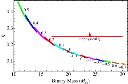
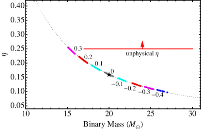
Fig. 2 shows the results for a binary with a total mass of 20 and mass ratio 1:4 (), i.e. a – binary, and matches calculated using the early aLIGO spectrum. We consider sources with a total spin in the range [-1,1] in steps of 0.1. For each configuration, we identify non-spinning waveforms which give a match of greater than 0.97 with the spinning source. When the binary spin is zero, the non-spinning model matches the target signal at the correct parameters (indicated by a star), and along a strip in the parameter space with a width of 5% in mass, and 10% in . When the binary contains spinning black holes, the non-spinning model matches the signal, but with a bias in the mass and mass ratio. The binary spins are indicated with different colours, labeled by the total spin of the binary. For large-spin signals there are no non-spinning waveforms that have a match above 0.97. When using the early aLIGO noise curve, the range of spins for which non-spinning waveforms have a match above 0.97 is . However, for spins above about , the best-match waveform has an unphysical value of the mass ratio . The curve of constant chirp mass is indicated by a dotted line.
The first thing to note is that, in all cases, the chirp mass of the best matched non-spinning waveform is very similar to the true chirp mass of the system. We can see from Fig. 2 that the high-match regions follow a line of constant chirp mass. In Fig. 3 we re-parameterize the results of Fig. 2 in terms of and . We see that, even though there is a strong degeneracy between and , the correct chirp mass falls within the high-match region for most values of spin. The deviation from the correct chirp mass is no more than % for large anti-aligned spins.
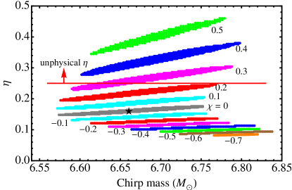
The second important point relates to the mass-spin degeneracy. For aligned-spin binaries (), the best match is obtained with a lower-mass, higher-mass-ratio model, while for anti-aligned spins, the best matched non-spinning waveform has a higher mass and lower mass-ratio. This is to be expected as aligned spins are expected to cause the system to “hang up” and chirp more slowly, mimicking a lower-mass signal.
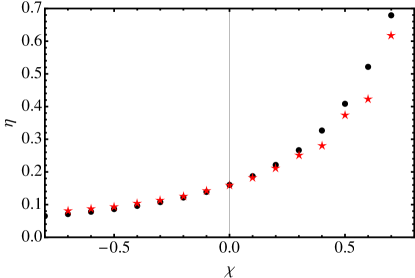
It is informative to return to the post-Newtonian phasing given in Eq. (5) to see whether the observed degeneracy matches what is theoretically expected. In low-mass binaries, the signal is dominated by the inspiral, which can be represented in a PN expansion, as described in Sec. III.1. The chirp mass is determined to high accuracy by the leading-order term in the PN expansion of the phase in the Fourier domain, and we can then solve Eq. (III.1) (with fixed chirp mass) to find the symmetric mass ratio that mimics the effect of the spin. We do this by solving (5) as a function of frequency (in the detector’s sensitive band) and then averaging over the values of that we obtain. Fig. 4 shows the symmetric mass ratio that corresponds to each value of the spin, as predicted from Eq. (III.1), and as found in the mismatch analysis of the phenomenological models that is shown in Fig. 2. We see that the PN estimate is remarkably close to that found for the full IMR models, at least for the binaries used in this example.
III.3 Evolution of noise curves
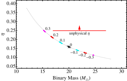
We present results for two design aLIGO configurations in Fig. 5: the no-signal-recycling (no-SRM) configuration and the final high-power zero-detuned sensitivity curve (final). Qualitatively, the results are quite similar for the no-SRM and final noise curves. Again spinning signals are recovered with a match above 0.97 using non-spinning templates, with a decrease in recovered mass for positive spin systems. The chirp mass is still well recovered. However, the detector’s extra sensitivity makes it easier to distinguish the spinning signals with a non-spinning model. The range of spins for which we can find a non-spinning signal with matches greater than 0.97 is now only for no-SRM and for the final configuration. We also see that each match region shrinks, although its location is unchanged. In moving from the early noise curve to no-SRM, the most significant sensitivity improvement is at low frequency, while the final configuration offers much greater high frequency sensitivity. The results for these two curves are quite comparable (and significantly better than the early curve) indicating that it is low frequency sensitivity that provides the biggest improvement in breaking the degeneracy. With the later noise curves, the variation of chirp mass between the spinning signal and non-spinning template is less than 1%. 111The figures may seem to indicate that a binary with total spin of 0.5 that would be detected by a non-spinning search in the early aLIGO configuration, but not later ones. This is of course not true: the final detector is roughly three times more sensitive at these masses, and so a signal with SNR 10 in early aLIGO would have an SNR of 30 in the final configuration. Even with a match of 0.9, this would still give an SNR of 27, and the match would be sufficient that it would pass any signal consistency tests.
IV Mass-spin degeneracy at higher masses
For black-hole binaries with masses greater than the merger and ringdown parts of the signal become increasingly important and contribute an ever increasing fraction of the signal-to-noise ratio. At higher masses, we do not expect the chirp mass to determine the waveform to such an extent as for the system and there is no a priori reason to expect that a degeneracy between mass and spin will persist.
We begin by considering a binary with mass ratio 1:4. At this mass, the merger and ringdown will provide a significant fraction of the signal to noise ratio. As a crude estimate of the effect, imagine that the inspiral part of the waveform is valid up to the innermost stable circular orbit (ISCO) of a point particle orbiting a Schwarzschild black hole, which is at 90 Hz for a binary. For the early aLIGO noise curve, the inclusion of the merger and ringdown will increase the SNR by a factor of 4. At the final aLIGO sensitivity, the improved low frequency response increases the contribution of the inspiral but the merger and ringdown still contribute a comparable SNR to the inspiral (so that the overall SNR is % higher, because they add in quadrature). Thus, there is no reason to expect that the chirp mass is still well recovered or that the degeneracy discussed previously still holds.
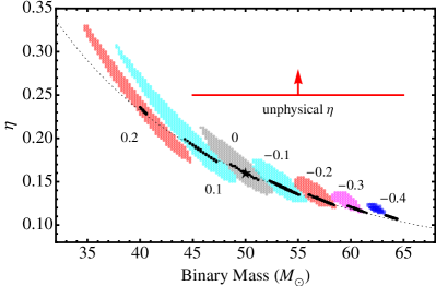
In Fig. 6 we again show the regions of the non-spinning parameter space which give a match greater than 0.97 with a spinning binary (with values of from -1 to 1 in steps of 0.1). Here, we show the results for both the early and final aLIGO spectra. The results are qualitatively similar to the binary with spinning signals well recovered by the non-spinning waveforms, and the chirp mass accurately recovered. The sizes of the regions are roughly consistent with the lower mass system, with a mass accuracy of % and range in of 0.05-0.1 for the early noise curve. For both early and design curves, signals with spins between 0.2 and -0.4 have matches above 0.97 with non-spinning waveforms. Interestingly the degeneracy still roughly follows the line of constant chirp mass, even though the merger and ringdown contributed significantly to the SNR of the signal.
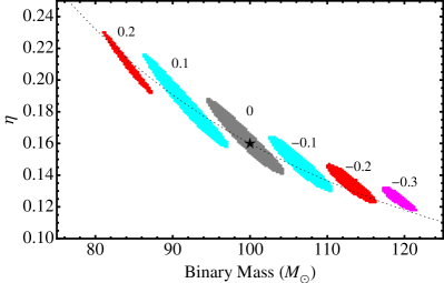
Next, we increase the mass to and repeat the analysis. At this mass, the point-particle ISCO is at 40 Hz, so there is essentially no power from the inspiral in the initial detectors, and only a small amount in the early aLIGO. Even at the final sensitivity, the merger and ringdown provide the vast majority of the SNR (a factor of 4 more than the inspiral). Thus one expects that it is really the merger that dictates the waveform as seen by the detector. Figure 7 shows results for 100, again with . For aLIGO at final design sensitivity, the curves are again lying pretty much along the line of constant chirp mass.
We do not show results for the early aLIGO sensitivity curve in Fig. 7, because the results depend strongly on the choice of model, either PhenomB or PhenomC. The variation of the two models with respect to the physical parameters is sufficiently large through merger and ringdown that they lead to qualitatively different results in our mismatch studies, when we use the early aLIGO noise curve, where the merger and ringdown contribute essentially all of the SNR. The two models were developed as pioneering models of aligned-spin IMR waveforms for use in searches, and for this we expect that they are sufficient; but their fidelity with respect to parameter estimation at high masses has not yet been tested, and should be a focus of future work to refine them.
V Parameter recovery
Once a black hole merger has been detected, we wish to extract the signal parameters as accurately as possible. Parameter estimation proceeds by identifying regions of parameter space which give a signal that is most consistent with the data. It stands to reason that these regions will contain waveforms that have a good match with the observed signal. Thus we might expect that confidence regions in parameter estimation are associated with regions of high match between signal and template. In this section, we show this expectation to hold in detail in the high-SNR limit and derive an expression for the value of the match that corresponds to a given confidence at a given SNR.
We begin by presenting the argument, using the Fisher matrix formulation, and then we use this connection to re-interpret our earlier results in terms of parameter recovery. We follow the formalism used Ref. Vallisneri (2008), but provide only a brief discussion of the Fisher matrix formalism, and refer the reader to the Ref. Vallisneri (2008) (and references therein) for more details.
V.1 Connection between mismatch and confidence regions
Let us assume that a signal is present in the data. The detector data is given as
| (6) |
To investigate signal recovery and parameter extraction at leading order, we Taylor expand the signal in a region of the true parameters () as
| (7) |
Here is used to denote the derivative of the waveform with respect to the paramters , which will include , , as well as the amplitude, phase and coalescence time that are maximized over in the match calculations.
The likelihood, for a given set of , is
| (8) |
Substituting the expressions for (6) and (7) into the above and keeping leading order terms gives
| (9) |
In the context of Bayesian parameter estimation, this can be recast in terms of a posterior probability distribution for the parameters using Bayes theorem:
| (10) |
where is the prior probability distribution for the parameters. In what follows, we use a uniform prior on the parameters. In general, such a prior will not be physically motivated but, for a detectable signal, the likelihood will be peaked in a small enough region of parameter space to make this approximation reasonable.
Given the above, we are interested in calculating the expected offset between the true parameters and the mean value from the posterior distribution. We also want to evaluate the size of a confidence region containing a given fraction of the posterior probability. These quantities give us two different measures of the expected accuracy of parameter recovery.
We begin by calculating the mean of the parameter as
| (11) |
Thus, the mean of the posterior distribution will be offset from the true parameter values due to the presence of noise. One way to characterize this is the expected size of the error waveform, as
| (12) |
where is the dimension of the parameter space and indicates the expectation value over many noise realizations. Thus, on average the difference between the true signal and “best fit” waveform will have an amplitude of .
Next, we turn our attention to confidence regions in parameter space — a region of parameter space that contains a given probability of the posterior distribution,
| (13) |
There are many ways to construct such a region, and one typically also requires the smallest possible region. To calculate confidence regions in the Fisher approximation, we begin by observing that the covariance between parameters is given as
| (14) |
Using this expression and Eq. (11), we can re-express the posterior distribution as
| (15) | |||||
Then, the minimum volume region which contains a fraction of the posterior probability is the one for which
| (16) |
where is the chi-square value for which there is probability of obtaining that value or larger, and denotes the degrees of freedom, determined by the number parameters included in . At leading order, the confidence interval contains all points for which the amplitude of the difference between the model and best fit waveforms lies below the given threshold.
There are six parameters in the aligned-spin waveform model: , , , , and . When calculating matches, we have maximized over the latter three parameters (amplitude, phase and time) and reported match over the three dimensional space of mass, mass ratio and spin. Thus, we have calculated the three dimensional matches , maximized over A, and . It is straightforward to re-cast our earlier results in terms of mismatches. To do this, we note that
| (17) |
When we restrict to the subspace of masses and spins, we can write the final term as the match between the waveforms.
By substituting Eq. (17) into Eq. (16), we see that the confidence region is defined by all points in the parameter space for which the match satisfies
| (18) |
where the value of is given by the dimension of the remaining parameter space. This expression gives us a straightforward way to re-interpret the match calculations presented earlier. For example, with a three dimensional parameter space, the 90% confidence region at a given SNR is given by:
| (19) |
which has the nice property that a match of 0.97 corresponds to a 90% confidence region at an SNR of 10. For a two dimensional parameter space, the right hand side is , meaning that a match of 0.97 corresponds to 90% confidence region at an SNR of 9.
We should note that there are numerous assumptions used in the derivation of these results. Most significantly, all of the Fisher matrix results consider only leading order effects and become less reliable at lower SNR, see e.g., Ref Vallisneri (2008) for a detailed discussion of the issues. When actually calculating confidence regions for a signal, detailed parameter estimation analyses calculate the posterior distribution (15) and integrate to find the region containing 90% of the probability. Here, we are using a hybrid approach: we use the result of the Fisher matrix calculation to decide the threshold on match required to define the given confidence region, but then calculate the match between waveforms exactly, without recourse to any approximations. Furthermore, we are maximizing the match over three dimensions, analytically for and and using a Fourier transform to search over time. Thus, we are only applying the Fisher result to the three dimensional subspace of mass, mass ratio and spin. Even there, we are merely using the calculation to determine the appropriate match threshold: the matches are calculated exactly. Consequently, the match regions should be in good agreement with the 90% confidence regions. We verified that for an SNR of 20, the region identified by our match criteria did contain 90% of the probability to within .
V.2 Implications for detectability and parameter estimation
Let us now return to the results of Sec. III and IV and use the relationship derived above to re-interpret the results in terms of confidence intervals. We can interpret Fig. 2 in two ways: in the context of either a non-spinning or spin-aligned templated search. If we were to perform a search with non-spinning templates and observe a , binary with non-spinning components with SNR 9, then the 90% confidence region would lie along a strip in the parameter space with a width of 5% in mass, and 10% in . For a binary containing the same mass black holes with spins of -0.5, the 90% confidence region would be of approximately the same size (5% in mass, and 10% in ) but centred at , .222Strictly speaking, if the best match between the signal and a model waveform is less than unity, the relation between match and confidence region in equation (18) must be modified to reflect this. The 90% confidence region will contain all points with a match of 0.97 or greater with the best fit model waveform. The same holds for other values of the spins: the reported statistical uncertainty in parameters is relatively small, while the systematic errors can be significant.
Alternatively, we can consider the three dimensional space of --. In that case, a match above 0.97 corresponds to a 90% confidence region at SNR of 10. Thus, for example, Fig. 2 shows that the 90% confidence region for a signal with and would contain waveforms with non-spinning components. Figures 3 to 7 can be interpreted in a similar manner. For higher SNRs, the confidence intervals shrink. At SNR 10 they correspond to matches of 0.97, SNR 20 to 0.992 and SNR 30 to 0.9965.
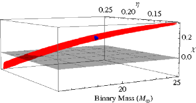
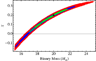
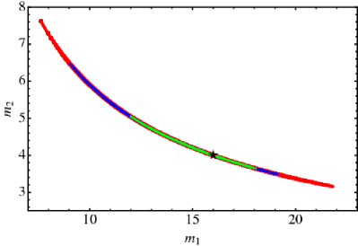
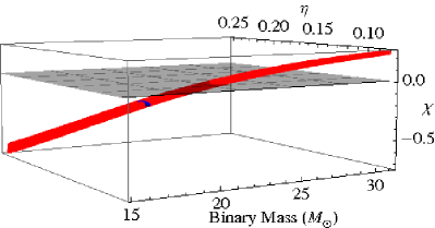
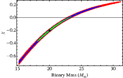
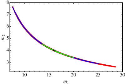
We can use the analysis of the previous section to estimate the 90% confidence intervals if we employ an aligned-spin model for parameter estimation. For signals with an SNR of 10, the three-dimensional confidence region in will correspond to matches greater than 0.97. In these cases we calculate the matches between a given aligned-spin signal, and all other aligned-spin model waveforms with varying mass, mass-ratio and total spin. In Fig. 8 we show the 0.97 match volume for a 20 1:4 binary with , using the final aLIGO noise curve. The top panel shows the full three-dimensional confidence region, and in the lower panels the results are projections onto the - and - planes, to aid the interpretation. Figure 9 shows similar results, but for a binary with .
Since our waveform model now includes spin, the best match is unity at the correct parameters. But from the figures we see that the 90% confidence region extends well beyond the correct parameters, and is far from the naive image conjured by the term “error ellipse”. We note in particular that this volume includes a region of the non-spinning binary parameter space; the intersection with the plane is consistent with the lower panel of Fig 5. If we were to estimate the parameters of this signal with an aligned-spin waveform model, we would find that the best-fit parameters indicated that the black holes were spinning, but could not rule out that they might in fact be non-spinning — or indeed have spins with the opposite orientation.
The reason for this large uncertainty in the parameters is that the SNR is low; it is only 10. For an SNR of 20, the 90% confidence interval corresponds to a match of above 0.992, and for an SNR of 30, the match must be above 0.9965. We see that for these higher SNRs, the confidence region shrinks. However, only at SNR 30 is a non-spinning signal excluded from the 90% confidence region for the case, and even at this SNR (which may be quite rare in aLIGO observations), the smaller mass is determined to within only 25%. When (Fig. 9, the 90% confidence region includes spins as high as , even when the SNR is 20. Note also that in these figures we have included only those portions of the confidence regions with , i.e., physically acceptable values; the confidence region would extend further in the upper two panels if the model were not constrained.
VI Conclusions
We have investigated the degeneracy between mass-ratio and spin in gravitational waveforms, going beyond inspiral models to include merger and ringdown signals from black-hole-binary mergers. We have used phenomenological inspiral-merger-ringdown (IMR) models to study the subset of the full binary parameter space that includes non-spinning black holes, and black holes with spins parallel or anti-parallel to the orbital angular momentum of the binary.
A degeneracy between mass-ratio and spin is already known for inspiral signals, which are relevant to ground-based gravitational-wave detectors for masses Buonanno et al. (2009); Brown et al. (2012). We find that this degeneracy persists at higher masses, where the detectors are also sensitive to the merger and ringdown. This means that in a GW search that uses only non-spinning binary templates (and this is computationally cheaper than including spin), the signal may still be detected, but the best-match template will have strongly biassed parameters. The mass-ratio–spin degeneracy follows lines of constant chirp mass, so the chirp mass will be recovered with reasonable accuracy, even up to high masses and for spinning signals. However, the total mass and mass-ratio of the best-matched template will be biased. As shown in Fig. 2, binaries with higher aligned spins will be recovered with a higher mass ratio, while those with anti-aligned spins will be recovered with a lower mass ratio. If we restrict the search to physical values of the symmetric mass ratio , then comparable-mass binaries whose spins are aligned with the orbital angular momentum will tend to be missed in the search. We show how these results will change as the detector evolves towards its final sensitivity in Fig. 5, and for higher masses in Figs. 6 and 7.
We also demonstrated that it is possible to use match calculations to estimate the confidence intervals in parameter estimation. For example, the 90% confidence region for the three-dimensional parameter space of (, , ) for signals with SNR 10 is given by the region with matches above . This allows us to estimate how the mass-rato–spin degeneracy will be reflected in parameter estimation. We show that for modest SNRs () it may be difficult to determine whether a binary includes spin, and even for high SNRs (), the mass-ratio–spin degeneracy impairs the accurate recovery in the individual black-hole masses; see Figs. 8 and 9. These results will affect the astrophysical conclusions that can be drawn from GW observations, and this will be explored in more detail in future work. It would also be interesting to exploit our knowledge of the mass-ratio–spin degeneracy in a jump proposal for Bayesian parameter-estimation codes van der Sluys et al. (2008a, b); Veitch and Vecchio (2010).
Our results are restricted to aligned-spin binaries, and will be affected by the inclusion of precession effects. At present, no complete inspiral-merger-ringdown model for precessing systems exists. It seems unlikely, however, that the inclusion of precession effects will reduce the size of the confidence regions. In general it is far more likely that increasing the dimensionality of the model parameter space will increase the parameter uncertainty, because the confidence regions will now correspond to lower matches. The recent results in Ref. Schmidt et al. (2012) show that precession effects have only a weak impact on the phasing, which suggests that while the inclusion of precession is unlikely to break the degeneracy discussed here, it is also unlikely to introduce an additional degeneracy in these three parameters. On the other hand, the inclusion of higher harmonics, which were ignored in this study, may improve the accuracy of the parameters. The net impact of these two effects remains to be studied in more detail in future work.
Acknowledgments
S.F. and M. H. were supported by Science and Technology Facilities Council grants ST/H008438/1 and ST/I001085/1. S.F. also acknowledges the support of the Royal Society. We are particularly grateful to P. Ajith, Sascha Husa and Frank Ohme for sharing with us their implementations of the PhenomB and PhenomC waveform families and match-calculation code. We also thank Chris Messenger and John Veitch for useful discussions.
References
- Abadie et al. (2010) J. Abadie et al. (LIGO Scientific), Class. Quant. Grav. 27, 173001 (2010), arXiv:1003.2480 [Unknown] .
- Dominik et al. (2012) M. Dominik, K. Belczynski, C. Fryer, D. Holz, E. Berti, T. Bulik, I. Mandel, and R. O’Shaughnessy, arXiv.org astro-ph.HE (2012).
- Ohme (2012) F. Ohme, Class.Quant.Grav. 29, 124002 (2012), arXiv:1111.3737 [gr-qc] .
- Hannam (2009) M. Hannam, Class. Quant. Grav. 26, 114001 (2009), arXiv:0901.2931 [gr-qc] .
- Ajith et al. (2012) P. Ajith, M. Boyle, D. A. Brown, B. Brugmann, L. T. Buchman, et al., Class.Quant.Grav. 29, 124001 (2012), arXiv:1201.5319 [gr-qc] .
- Ajith et al. (2011) P. Ajith, M. Hannam, S. Husa, Y. Chen, B. Bruegmann, et al., Phys.Rev.Lett. 106, 241101 (2011), arXiv:0909.2867 [gr-qc] .
- Santamaria et al. (2010) L. Santamaria, F. Ohme, P. Ajith, B. Bruegmann, N. Dorband, et al., Phys.Rev. D82, 064016 (2010), arXiv:1005.3306 [gr-qc] .
- Pan et al. (2010) Y. Pan, A. Buonanno, L. T. Buchman, T. Chu, L. E. Kidder, et al., Phys.Rev. D81, 084041 (2010), arXiv:0912.3466 [gr-qc] .
- Schmidt et al. (2012) P. Schmidt, M. Hannam, and S. Husa, (2012), arXiv:1207.3088 [gr-qc] .
- Cutler and Flanagan (1994a) C. Cutler and E. E. Flanagan, Phys.Rev. D49, 2658 (1994a), arXiv:gr-qc/9402014 [gr-qc] .
- Poisson and Will (1995) E. Poisson and C. M. Will, Phys.Rev. D52, 848 (1995), arXiv:gr-qc/9502040 [gr-qc] .
- Abadie et al. (2012) J. Abadie et al. (LIGO Scientific Collaboration and Virgo Collaboration), Phys. Rev. D 85, 082002 (2012), arXiv:1111.7314 .
- Abadie et al. (2011) J. Abadie et al. (LIGO Scientific Collaboration and Virgo Collaboration), Phys. Rev. D 83, 122005 (2011), arXiv:1102.3781 .
- Brown et al. (2012) D. A. Brown, I. Harry, A. Lundgren, and A. H. Nitz, (2012), arXiv:1207.6406 [gr-qc] .
- van der Sluys et al. (2008a) M. van der Sluys et al., Classical and Quantum Gravity 25, 184011 (2008a), arXiv:0805.1689 [gr-qc] .
- van der Sluys et al. (2008b) M. V. van der Sluys et al., The Astrophysical Journal Letters 688, L61 (2008b), arXiv:0710.1897 .
- Veitch and Vecchio (2010) J. Veitch and A. Vecchio, Phys. Rev. D 81, 062003 (2010), arXiv:0911.3820 [astro-ph.CO] .
- Feroz et al. (2009) F. Feroz, M. P. Hobson, and M. Bridges, Monthly Notices of the Royal Astronomical Society 398, 1601 (2009), arXiv:0809.3437 .
- (19) “LSC Algorithm Library software packages lal, lalwrapper, and lalapps,” .
- Ajith et al. (2007a) P. Ajith, S. Babak, Y. Chen, M. Hewitson, B. Krishnan, et al., Class.Quant.Grav. 24, S689 (2007a), arXiv:0704.3764 [gr-qc] .
- Ajith et al. (2008) P. Ajith, S. Babak, Y. Chen, M. Hewitson, B. Krishnan, et al., Phys.Rev. D77, 104017 (2008), 22 Pages, 14 Figures, arXiv:0710.2335 [gr-qc] .
- Ajith (2008) P. Ajith, Class.Quant.Grav. 25, 114033 (2008), arXiv:0712.0343 [gr-qc] .
- Ajith et al. (2007b) P. Ajith et al., (2007b), arXiv:0709.0093 [gr-qc] .
- Abbott et al. (2009) B. Abbott et al. (LIGO Scientific), Rept. Prog. Phys. 72, 076901 (2009), arXiv:0711.3041 [gr-qc] .
- Shoemaker (2009) D. Shoemaker (the Advanced LIGO Team), “Advanced LIGO Reference Design,” (2009), [LIGO-M060056].
- Harry and the LIGO Scientific Collaboration (2010) G. M. Harry and the LIGO Scientific Collaboration, Class. Quant. Grav. 27, 084006 (2010).
- Shoemaker, David and Losurdo, Giovanni (2010) Shoemaker, David and Losurdo, Giovanni, Possible Scenarios for Commissioning and Early Observing with the Second Generation Detectors, Tech. Rep. LIGO-G10001760-v7 (LIGO Project, 2010).
- The LIGO Scientific Collaboration (2009) The LIGO Scientific Collaboration, Advanced LIGO Anticipated Sensitivity Curves, Tech. Rep. LIGO-T0900288-v3 (LIGO Project, 2009).
- Cutler and Flanagan (1994b) C. Cutler and E. E. Flanagan, Phys. Rev. D 49, 2658 (1994b).
- Babak et al. (2006) S. Babak, R. Balasubramanian, D. Churches, T. Cokelaer, and B. S. Sathyaprakash, Classical and Quantum Gravity 23, 5477 (2006).
- Babak et al. (2012) S. Babak, R. Biswas, P. Brady, D. Brown, K. Cannon, et al., (2012), arXiv:1208.3491 [gr-qc] .
- Lindblom et al. (2008) L. Lindblom, B. Owen, and D. Brown, Physical Review D 78, 124020 (2008).
- Ajith (2011) P. Ajith, Phys.Rev. D84, 084037 (2011), arXiv:1107.1267 [gr-qc] .
- Boyle et al. (2009) M. Boyle, D. A. Brown, and L. Pekowsky, Class.Quant.Grav. 26, 114006 (2009), arXiv:0901.1628 [gr-qc] .
- Vallisneri (2008) M. Vallisneri, Physical Review D 77, 42001 (2008).
- Buonanno et al. (2009) A. Buonanno, B. Iyer, E. Ochsner, Y. Pan, and B. Sathyaprakash, Phys.Rev. D80, 084043 (2009), arXiv:0907.0700 [gr-qc] .