Study of Hund’s rule coupling in models of magnetic impurities and quantum dots
Abstract
Studies of the effects of the Hund’s rule coupling in multiple orbit impurities or quantum dots using different models have led to quite different predictions for the Kondo temperature as a function of . We show that the differences depend on whether or not the models conserve orbital angular momentum about the impurity site. Using numerical renormalization group (NRG) calculations, we deduce the renormalized parameters for the Fermi liquid regime, and show that, despite the differences between the models, the low energy fixed point in the strong correlation regime is universal with a single energy scale , and just two renormalized interaction parameters, a renormalized single orbital term, , and renormalized Hund’s rule term, .
pacs:
72.10.F,72.10.A,73.61,11.10.GI Introduction
The role of the Hund’s rule coupling has been investigated for magnetic impurities and quantum dots by a number of authors starting from rather different models Sch67 ; NC09 ; NCH10s ; PB05 ; SNOHT12 . This has led to different predictions for the behavior of the Kondo temperature in these systems as a function of . As a result it is not clear whether or not the models may also differ in their predictions for their low energy behavior. We investigate this question by applying a combination of the numerical renormalization group (NRG) and renormalized perturbation theory (RPT) to some of these different models. From an analysis of single particle excitations about the NRG low energy fixed point we can obtain an accurate estimate of the Kondo temperature in all cases. We can also calculate the renormalized interaction parameters at this fixed point and compare them for the different models. This information can be used to deduce the low temperature specific heat coefficient, spin and charge susceptibilities and low energy dynamical behavior for the models in all parameter regimes.
A model of a magnetic impurity with -fold degenerate orbitals interaction with a bath of conduction electrons will in general require quite a large number of parameters to describe the interactions between the electrons in these orbitals for various filling factors, and their interaction with the conduction electrons of the host metal. To understand the basic physics of these models a number of different models, using a restricted set of parameters, have been used. One of these models was introduced by Yoshimori (model 1) where the interactions between electrons in the impurity orbitals were specified by just two parameters Yos76 , a local Coulomb interaction and an inter-orbital exchange interaction . The Hamiltonian of the model takes the form,
| (1) |
| (2) | |||||
where , , are creation and annihilation operators for an electron in an impurity state with total angular momentum quantum number , and -component , and spin component . The impurity level in a magnetic field we take as , where () and () and is the chemical potential, and the Bohr magneton. The creation and annihilation operators , are for partial wave conduction electrons with energy . The hybridization matrix element for impurity levels with the conduction electron states is . We denote the hybridization width factor by , which we can take to be a constant in the wide flat band limit. The remaining part of the Hamiltonian, describes the interaction between the electrons in the impurity state,
| (3) | |||||
This model can be used to describe transition metal impurities, such as Fe or Mn, in a metallic host in the absence of spin orbit or crystal field splittings. The model can be interpreted more generally with as a channel index taking values where is the number of channels. The Hund’s rule term tends to align the electrons on the impurity site such that for large and large the impurity state will correspond to a spin .
A different -fold model has been studied recently by Nevidomskyy and Coleman NC09 (model 2) which also includes a Hund’s rule interaction. This model is characterized by just two interaction terms, an inter-orbital Hund’s rule exchange interaction and an Kondo form of exchange interaction between the impurity electrons and the conduction electrons, so that the Hamiltonian takes the form,
| (4) | |||||
There are significant differences between models 1 and 2, which can be seen more clearly if we restrict the discussion to the case , when model 1 can be written in a more usual form with the exchange interaction written in terms of spin operators,
| (5) |
with . We generalize the model by taking as an independent parameter, and refer to the model in this generalized form as model 3. It has been used in this form to describe the interactions in certain double quantum dotsSNOHT12 .
We consider, first of all, model 3 in the limit with . In this case there is no interaction or hybridization between the two channels and the model is equivalent to two independent Anderson models. In the strong coupling regime with particle-hole symmetry it can be converted into model 2 () via a Schrieffer-Wolff transformation with . If the first order correction term in is included in this limit, then model 3 can be seen to be essentially equivalent to model 2 in Eq. (4) for .
However, for , and in Eq. (5), corresponding to the Yoshimori model (model 1), there is an interaction between the two channels. In this case the orbital index can be combined with the spin index into a single index running over 4 values and the model can be shown to have SU(4) symmetry, corresponding to conservation of both spin and orbital angular momentum. In the particle-hole localized limit with , it can be transformed via a Schrieffer-Wolff transformation (which takes into account virtual excitations from the 2-electron, six-fold degenerate, ground state of the impurity to 1-electron and 3-electron excited states) into an SU(4) Kondo model with with a six dimensional representation for the local SU(4) operatorsNCH10s . Hence models 1 and 2 are quite different in the Kondo regime for . For general , in the Kondo regime when , model 1 reduces to an SU(2n) Kondo model and model 2 to independent SU(2) Kondo models. This reflects the important difference that model 1 is invariant under orbital as well as spin rotation, whereas model 2, and model 3 when , are invariant under spin rotation only. This can be verified explicitly by considering the commutator of the generator, , with the Hamiltonian of model 3. This difference could have consequences for the low energy behavior of these models which we consider in the next section.
II Low energy Fermi liquid regime
The conservation of both angular momentum and spin in model 1 permitted Yoshimori Yos76 to derive two Ward identities for interaction vertex part at zero frequency. This interaction vertex can be interpretated in terms of a renormalized interaction between the quasiparticles of a Fermi liquidNCH10s described by the Hamiltonian, , where
| (6) |
and
| (7) | |||||
This effective model is of the same form as the original model defined in Eqs. (2) and (3) with the difference that the interaction terms have to be normal ordered. The brackets indicate the normal ordering of the operator with respect to the ground state of the interacting system, which plays the role of the vacuum. This term only comes into play when more than one quasiparticle is created from the vacuum.
From the Ward identitiesYos76 ; YZ82 ; NCH10s exact expressions can be derived for the impurity charge, spin and orbital susceptibilities, , , and , at ,
| (8) |
| (9) |
| (10) |
where is the free quasiparticle density of states per single spin and channel,
| (11) |
The impurity contribution to the specific heat coefficient is also given exactly by and the Wilson ratio is given by
| (12) |
In the localized limit with particle-hole symmetry (), the charge susceptibility is suppressed so we can equate to zero. Similarly when is large the orbital susceptibility will be suppressed so that can also be equated to zero. Then from Eqs. (8) and (10) we obtain for the spin susceptibility,
| (13) |
where and , and the relation between the renormalized parameters,
| (14) |
As angular momentum is not conserved for model 2, and model 3 if , the question arises as to whether the low energy fixed point of this model can be described by a quasiparticle Hamiltonian with renormalized parameters, similar to that given in Eqs. (6) and (7), and if so, does the relation given in Eq. (14) hold when is large?
To examine this question we extend our earlier NRG calculationsNCH10s of the renormalized parameters for model 1 to models 2 and 3 for the case . We can test the hypothesis that the low temperature behaviour of all three models can be described by a quasiparticle Hamiltonian in terms a set of renormalized parameters, , , and . We restrict our calculations to the particle-hole symmetric case and take in the one-electron part of the Hamiltonian given in Eq. (2). In the NRG calculations we used for the discretization parameter and half-bandwidth , and approximately 4000 states were retained at each iteration. The value was used for models 1 and 3.
III Calculation of renormalized parameters and Susceptibilities
The renormalized parameters that describe the quasiparticles and their interactions can be deduced from an analysis of the low energy NRG fixed point. The parameters and can be deduced by fitting the lowest single particle and hole excitations from the NRG ground state to those of a non-interacting Anderson model. The interaction parameters, , and , can be deduced from the lowest two-particle excitations, in the same channel for , and different channels for and . We have analysed the fixed point in the same way for all the models, including model 2. Details of these calculations were given in earlier workHOM04 ; NCH10s ; NCH10a ; NCH12b so we shall just quote the results of such an analysis here.
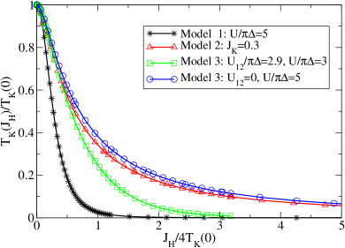
We use the relation, to deduce the Kondo temperature in the particle-hole symmetric case for all the models. The results for as a function of are shown in Fig. 1 for particular parameter sets for the three models. For model 1 with , the value of falls of rapidly with increase of . Results for this case were presented in earlier workNCH10s , and shown to decrease exponentially with a fit with . This exponential dependence is to be expected from a Schrieffer-Wolff transformation in the regime when and is large, when the ground state of the isolated impurity is a two electron spin triplet state. When virtual excitations to local states with one more or one less electron are taken into this leads to a spin 1 Kondo model with an effective antiferromagnetic coupling , giving exponential factor in in the resulting Kondo temperature , where is the density of states of the conduction electrons at the Fermi level.
The results for model 2 are for the case with , and are seen to decrease much more slowly with increase of and appear to level off for larger values of . However, the initial values of are rather different for the two models. As model 2 in this limit reduces to -independent SU(2) Kondo models the Kondo temperature is given by . In this limit, on the other hand, model 1 corresponds to an SU(2n) Kondo model, which has a Kondo temperature , so for the same coupling is likely to be significantly larger than that for the SU(2) model.
The results for model 3 with , , also shown in Fig. 1, are very similar to those of model 2. This is not surprising because because, as noted earlier, when and it can be transformed into model 2 (with ) via a Schrieffer-Wolff transformation when is large, and adding the first order correction term in gives essentially model 2.
Another parameter set for model 3 with , , is shown in Fig. 1. In this case there is still a marked fall off of with but intermediate between the other cases shown.
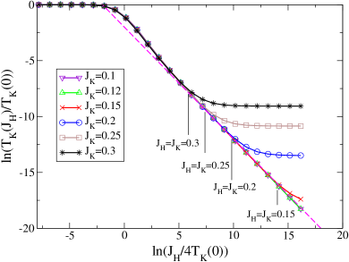
In Fig. 2 we examine the dependence of on for model 2 in more detail by plotting versus for a range of values for the Kondo coupling, . All the results fall on a universal curve provided . At the curves begin to deviate and develop a plateau for for the larger values of , . Plateaus also develop for the smaller values of for beyond the range shown in Fig. 2. We can compare these results with the scaling relation derived to one loop order for this model by Nevidomskyy and Coleman NC09 (Eq. (11) in their paper with ) for intermediate values of the Hund’s rule coupling , which predicts . This would correspond to a linear behavior in the log-log plot in Fig. 2 with a slope . The dashed line Fig. 2 corresponding to does fit the curves over a substantial range, particularly for the smaller values of . However, a linear fit to the range for larger values of would give a larger slope with , with varying depending on the fitting range chosen. The linear fit with begins at values of .
When and the two impurity spins are locked together, model 2 should also be equivalent to an effective Kondo model with the electrons in the two channels coupled to a spin . For the general -channel model this Hamiltonian would take the form,
| (15) |
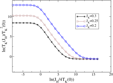
with an effective coupling of a spin to the conduction electrons. In the limit the result, , derived by Schrieffer Sch67 for model 2 should be valid. The Kondo temperature of the model with would then be given by , neglecting any dependence of the prefactors on . The corresponding result for the model with , , again neglecting any dependence of the prefactors on , would then imply . We can test this result for by modifying the plot given in Fig. 2 and plot instead versus . The results are shown in Fig. 3 for , It can be seen for the cases shown that, in the regime , the ratios of become independent of the value of which implies that, for , . This gives a clear criterion for the Schrieffer relationSch67 , , to hold.
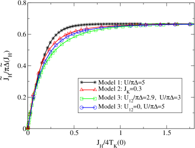
In Fig. 4 we plot the ratio of the renormalized parameters, versus for the different models for the parameter sets given in Fig. 1. We can see that all the curves asyptotically approach the value predicted in Eq. (14), on increasing . Though they approach this value at different rates they are all very close to the limiting value for . This clearly shows that the crossover to susceptibility corresponding to a spin 1 Kondo model, as given in Eq. (13), on increasing occurs on a scale . The regime for model 2 corresponds to the scaling regime of Nevidomskyy and Coleman NC09 where the low temperature behaviour can be described by a spin 1 Kondo model before the crossover to the regime where becomes independent of , and the Schrieffer resultSch67 , , holds.
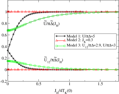
The remaining renormalized parameter ratios, and , that characterize the low energy fixed point, are shown in Fig. 5 for the different models as a function of . For model 1 with the charge fluctuations are suppressed , so from Eq. (8) when () for we get . As for this model when , we also predict the result . These are confirmed in the results given in Fig. 5. When is increased and the orbital fluctuations are also suppressed we get the results for this model given in Eq. (14), which imply that in this limit , and the NRG calculations confirm these results.
The NRG results for model 2 give and for all values of . We also obtain the same results for model 3 (not shown) for the case , . This is not surprising because, as noted earlier, when and , model 3 and model 2 are very similar.
Finally in Fig. 5 results are shown for model 3 for the case and . To test the predictions in this case, the expression for given in Eq. (8) must be generalized as it assumes the relation. . As both charge and spin are conserved in model 3, from the corresponding Ward indentities, exact results for the charge and spin susceptibilities can be derived. For the generalized expression for the charge susceptibility takes the form,
| (16) |
As the charge fluctations are suppressed for model 3 with and , Eq. (16) predicts the result , which is satisfied in the results shown in Fig. 5 for all values of . Though both and are non-zero for , as is increased , in line with the result in Eq. (14).
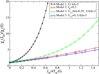
The expressions for spin susceptibility and Wilson ratio for model 3 with remain unchanged from those given in Eqs. (9) and (12). To calculate the impurity spin susceptibility for the models and parameters sets used in the other plots we substitute the renormalized parameters into Eq. (9) and give the results in Fig. 6. The exponential decrease of the Kondo temperature with increase of gives a dramatic rise in for model 1 compared with the corresponding results for models 2 and 3. However, the change in the corresponding Wilson ratios on increasing from zero is much less dramatic. For model 1 with , increases from for to for large , and for model 2 from to over the same range.
Yoshimori Yos76 derived an exact result for the low temperature impurity contribution to the resistivity for model 1 in the particle-hole symmetric case and . In terms of the renormalized parameters, the result is
| (17) |
where is given by
| (18) |
and . For models 2 and 3 for the case this result can be generalized using renormalized perturbation to second order in the renormalized interaction vertices for the impurity self-energyNCH10s ; NCH12a ; NCH12b to give
| (19) |
which takes the value in the regime where Eq. (14) holds.
IV Conclusions
We have shown that we can get very different results for the Kondo temperature as a function of the Hund’s rule coupling depending on how this term is included in a model of a magnetic impurity. The physically most relevant model for a magnetic impurity with -fold degenerate states in the absence of crystal field or spin-orbit splitting should be the one introduced by Yoshimori Yos76 which conserves orbital angular momentum about the impurity site, or the generalizations of this model considered by Mihály and ZawadowskyMZ78 , and Yoshimori and Zawadowski YZ82 , where off-diagonal matrix elements of the scattering between orbital channels are included, subject to the condition of overall conservation of angular momentum. These matrix elements omitted from the Yoshimori model have been shown by Noziéres and Blandin NB80 not to affect the results in low temperature Fermi liquid regime, nor the derivation of the impurity spin and orbital susceptibilities based on the Ward identities deduced from conservation of spin and orbital angular momentumYZ82 . The restriction to models where angular momentum is conserved about the impurity site might not be appropriate to all situations, such as use of the model 3 (given in Eq. (4)) to describe the interaction between two quantum dotsSNOHT12 . We have studied in particular the model used by Nevidomskyy and Coleman NC09 for the case and, for the smaller values of , verified their scaling equation when the Hund’s rule coupling becomes strong enough to lock the individual spins to form an effective spin 1 coupled to the conduction electrons with an effective Kondo coupling . We also found the point where this scaling crosses over to the regime considered by SchriefferSch67 , where and the becomes independent of .
We find that the low temperature behaviour of all the models considered can be described in terms of a quasiparticle Hamiltonian with renormalized parameters, which, for the case , can be deduced from an analysis of the low energy fixed point of the NRG calculation. We have shown that, despite the differences between the models, in the strong Hund’s rule regime, just two interaction parameters are required, a renormalized interaction , within each impurity orbital, and a renormalized Hund’s rule interaction between electrons in different orbitals , which can both be expressed in terms of the Kondo temperature, and .
Acknowledgment
We thank Daniel Crow and Johannes Bauer for helpful discussions. This work has been supported in part by the EPSRC Mathematics Platform grant EP/1019111/1.
References
- (1) J. R. Schrieffer, Journal of Applied Physics 38, 1143 (1967).
- (2) A. H. Nevidomskyy and P. Coleman, Phys. Rev. Lett. 103, 147205 (2009).
- (3) Y. Nishikawa, D. J. G. Crow, and A. C. Hewson, Phys. Rev. B 82, 115123 (2010).
- (4) T. Pruschke and R. Bulla, Eur. Phys. J. B 44, 217 (2005).
- (5) R. Sakano, Y. Nishikawa, A. Oguri, A. C. Hewson, and S. Taruchi, Phys. Rev. Lett. 108, 266401 (2012).
- (6) A. Yoshimori, Prog. Theor. Phys. 55, 66 (1976).
- (7) A. Yoshimori and A. Zawadowski, J. Phys. C 15, 5421 (1982).
- (8) A. C. Hewson, A. Oguri, and D. Meyer, Eur. Phys. J. B 40, 177 (2004).
- (9) Y. Nishikawa, D. J. G. Crow, and A. C. Hewson, Phys. Rev. B 82, 245109 (2010).
- (10) Y. Nishikawa, D. J. G. Crow, and A. C. Hewson, Phys. Rev. B 86, 123134 (2012).
- (11) Y. Nishikawa, D. J. G. Crow, and A. C. Hewson, Phys. Rev. Lett. 108, 056402 (2012).
- (12) L. Mihály and A. Zawadowsky, J. Physique Lett. 39, L483 (1978).
- (13) P. Nozières and A. Blandin, J. Physique 41, 193 (1980).