Deep Gaussian Processes
Andreas C. Damianou Neil D. Lawrence Dept. of Computer Science & Sheffield Institute for Translational Neuroscience, University of Sheffield, UK
Abstract
In this paper we introduce deep Gaussian process (GP) models. Deep GPs are a deep belief network based on Gaussian process mappings. The data is modeled as the output of a multivariate GP. The inputs to that Gaussian process are then governed by another GP. A single layer model is equivalent to a standard GP or the GP latent variable model (GP-LVM). We perform inference in the model by approximate variational marginalization. This results in a strict lower bound on the marginal likelihood of the model which we use for model selection (number of layers and nodes per layer). Deep belief networks are typically applied to relatively large data sets using stochastic gradient descent for optimization. Our fully Bayesian treatment allows for the application of deep models even when data is scarce. Model selection by our variational bound shows that a five layer hierarchy is justified even when modelling a digit data set containing only 150 examples.
1 Introduction
Probabilistic modelling with neural network architectures constitute a well studied area of machine learning. The recent advances in the domain of deep learning (Hinton and Osindero, 2006; Bengio et al., 2012) have brought this kind of models again in popularity. Empirically, deep models seem to have structural advantages that can improve the quality of learning in complicated data sets associated with abstract information (Bengio, 2009). Most deep algorithms require a large amount of data to perform learning, however, we know that humans are able to perform inductive reasoning (equivalent to concept generalization) with only a few examples (Tenenbaum et al., 2006). This provokes the question as to whether deep structures and the learning of abstract structure can be undertaken in smaller data sets. For smaller data sets, questions of generalization arise: to demonstrate such structures are justified it is useful to have an objective measure of the model’s applicability.
The traditional approach to deep learning is based around binary latent variables and the restricted Boltzmann machine (RBM) (Hinton, 2010). Deep hierarchies are constructed by stacking these models and various approximate inference techniques (such as contrastive divergence) are used for estimating model parameters. A significant amount of work has then to be done with annealed importance sampling if even the likelihood111We use emphasis to clarify we are referring to the model likelihood, not the marginal likelihood required in Bayesian model selection. of a data set under the RBM model is to be estimated (Salakhutdinov and Murray, 2008). When deeper hierarchies are considered, the estimate is only of a lower bound on the data likelihood. Fitting such models to smaller data sets and using Bayesian approaches to deal with the complexity seems completely futile when faced with these intractabilities.
The emergence of the Boltzmann machine (BM) at the core of one of the most interesting approaches to modern machine learning is very much a case of a the field going back to the future: BMs rose to prominence in the early 1980s, but the practical implications associated with their training led to their neglect until families of algorithms were developed for the RBM model with its reintroduction as a product of experts in the late nineties (Hinton, 1999).
The computational intractabilities of Boltzmann machines led to other families of methods, in particular kernel methods such as the support vector machine (SVM), to be considered for the domain of data classification. Almost contemporaneously to the SVM, Gaussian process (GP) models (Rasmussen and Williams, 2006) were introduced as a fully probabilistic substitute for the multilayer perceptron (MLP), inspired by the observation (Neal, 1996) that, under certain conditions, a GP is an MLP with infinite units in the hidden layer. MLPs also relate to deep learning models: deep learning algorithms have been used to pretrain autoencoders for dimensionality reduction (Hinton and Salakhutdinov, 2006). Traditional GP models have been extended to more expressive variants, for example by considering sophisticated covariance functions (Durrande et al., 2011; Gönen and Alpaydin, 2011) or by embedding GPs in more complex probabilistic structures (Snelson et al., 2004; Wilson et al., 2012) able to learn more powerful representations of the data. However, all GP-based approaches considered so far do not lead to a principled way of obtaining truly deep architectures and, to date, the field of deep learning remains mainly associated with RBM-based models.
The conditional probability of a single hidden unit in an RBM model, given its parents, is written as
where here is the output variable of the RBM, is the set of inputs being conditioned on and . The conditional density of the output depends only on a linear weighted sum of the inputs. The representational power of a Gaussian process in the same role is significantly greater than that of an RBM. For the GP the corresponding likelihood is over a continuous variable, but it is a nonlinear function of the inputs,
where is a Gaussian density with mean and variance . In this case the likelihood is dependent on a mapping function, , rather than a set of intermediate parameters, . The approach in Gaussian process modelling is to place a prior directly over the classes of functions (which often specifies smooth, stationary nonlinear functions) and integrate them out. This can be done analytically. In the RBM the model likelihood is estimated and maximized with respect to the parameters, . For the RBM marginalizing is not analytically tractable. We note in passing that the two approaches can be mixed if which recovers a GP classification model. Analytic integration is no longer possible though, and a common approach to approximate inference is the expectation propagation algorithm (see e.g. Rasmussen and Williams, 2006). However, we don’t consider this idea further in this paper.
Inference in deep models requires marginalization of as they are typically treated as latent variables222They can also be treated as observed, e.g. in the upper most layer of the hierarchy where we might include the data label., which in the case of the RBM are binary variables. The number of the terms in the sum scales exponentially with the input dimension rendering it intractable for anything but the smallest models. In practice, sampling and, in particular, the contrastive divergence algorithm, are used for training. Similarly, marginalizing in the GP is analytically intractable, even for simple prior densities like the Gaussian. In the GP-LVM (Lawrence, 2005) this problem is solved through maximizing with respect to the variables (instead of the parameters, which are marginalized) and these models have been combined in stacks to form the hierarchical GP-LVM (Lawrence and Moore, 2007) which is a maximum a posteriori (MAP) approach for learning deep GP models. For this MAP approach to work, however, a strong prior is required on the top level of the hierarchy to ensure the algorithm works and MAP learning prohibits model selection because no estimate of the marginal likelihood is available.
There are two main contributions in this paper. Firstly, we exploit recent advances in variational inference (Titsias and Lawrence, 2010) to marginalize the latent variables in the hierarchy variationally. Damianou et al. (2011) has already shown how using these approaches two Gaussian process models can be stacked. This paper goes further to show that through variational approximations any number of GP models can be stacked to give truly deep hierarchies. The variational approach gives us a rigorous lower bound on the marginal likelihood of the model, allowing it to be used for model selection. Our second contribution is to use this lower bound to demonstrate the applicability of deep models even when data is scarce. The variational lower bound gives us an objective measure from which we can select different structures for our deep hierarchy (number of layers, number of nodes per layer). In a simple digits example we find that the best lower bound is given by the model with the deepest hierarchy we applied (5 layers).
The deep GP consists of a cascade of hidden layers of latent variables where each node acts as output for the layer above and as input for the layer below—with the observed outputs being placed in the leaves of the hierarchy. Gaussian processes govern the mappings between the layers.
A single layer of the deep GP is effectively a Gaussian process latent variable model (GP-LVM), just as a single layer of a regular deep model is typically an RBM. (Titsias and Lawrence, 2010) have shown that latent variables can be approximately marginalized in the GP-LVM allowing a variational lower bound on the likelihood to be computed. The appropriate size of the latent space can be computed using automatic relevance determination (ARD) priors (Neal, 1996). Damianou et al. (2011) extended this approach by placing a GP prior over the latent space, resulting in a Bayesian dynamical GP-LVM. Here we extend that approach to allow us to approximately marginalize any number of hidden layers. We demonstrate how a deep hierarchy of Gaussian processes can be obtained by marginalising out the latent variables in the structure, obtaining an approximation to the fully Bayesian training procedure and a variational approximation to the true posterior of the latent variables given the outputs. The resulting model is very flexible and should open up a range of applications for deep structures 333A preliminary version of this paper has been presented in (Damianou and Lawrence, 2012)..
2 The Model
We first consider standard approaches to modeling with GPs. We then extend these ideas to deep GPs by considering Gaussian process priors over the inputs to the GP model. We can apply this idea recursively to obtain a deep GP model.
2.1 Standard GP Modelling
In the traditional probabilistic inference framework, we are given a set of training input-output pairs, stored in matrices and respectively, and seek to estimate the unobserved, latent function , responsible for generating given . In this setting, Gaussian processes (GPs) (Rasmussen and Williams, 2006) can be employed as nonparametric prior distributions over the latent function . More formally, we assume that each datapoint is generated from the corresponding by adding independent Gaussian noise, i.e.
| (1) |
and is drawn from a Gaussian process, i.e. . This (zero-mean) Gaussian process prior only depends on the covariance function operating on the inputs . As we wish to obtain a flexible model, we only make very general assumptions about the form of the generative mapping and this is reflected in the choice of the covariance function which defines the properties of this mapping. For example, an exponentiated quadratic covariance function, , forces the latent functions to be infinitely smooth. We denote any covariance function hyperparameters (such as of the aforementioned covariance function) by . The collection of latent function instantiations, denoted by , is normally distributed, allowing us to compute analytically the marginal likelihood 444All probabilities involving should also have in the conditioning set, but here we omit it for clarity.
| (2) |
Gaussian processes have also been used with success in unsupervised learning scenarios, where the input data are not directly observed. The Gaussian process latent variable model (GP-LVM) (Lawrence, 2005, 2004) provides an elegant solution to this problem by treating the unobserved inputs as latent variables, while employing a product of independent GPs as prior for the latent mapping. The assumed generative procedure takes the form: where is again Gaussian with variance and with . Given a finite data set, the Gaussian process priors take the form
| (3) |
which is a Gaussian and, thus, allows for general non-linear mappings to be marginalised out analytically to obtain the likelihood , analogously to equation (2.1).
2.2 Deep Gaussian Processes
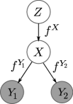
Our deep Gaussian process architecture corresponds to a graphical model with three kinds of nodes, illustrated in figure 11: the leaf nodes which are observed, the intermediate latent spaces , where is the number of hidden layers, and the parent latent node . The parent node can be unobserved and potentially constrained with a prior of our choice (e.g. a dynamical prior), or could constitute the given inputs for a supervised learning task. For simplicity, here we focus on the unsupervised learning scenario. In this deep architecture, all intermediate nodes act as inputs for the layer below (including the leaves) and as outputs for the layer above. For simplicity, consider a structure with only two hidden units, as the one depicted in figure 11. The generative process takes the form:
| (4) |
and the intermediate node is involved in two Gaussian processes, and , playing the role of an input and an output respectively: . This structure can be naturally extended vertically (i.e. deeper hierarchies) or horizontally (i.e. segmentation of each layer into different partitions of the output space), as we will see later in the paper. However, it is already obvious how each layer adds a significant number of model parameters () as well as a regularization challenge, since the size of each latent layer is crucial but has to be a priori defined. For this reason, unlike Lawrence and Moore (2007), we seek to variationally marginalise out the whole latent space. Not only this will allow us to obtain an automatic Occam’s razor due to the Bayesian training, but also we will end up with a significantly lower number of model parameters, since the variational procedure only adds variational parameters. The first step to this approach is to define automatic relevance determination (ARD) covariance functions for the GPs:
| (5) |
This covariance function assumes a different weight for each latent dimension and this can be exploited in a Bayesian training framework in order to “switch off” irrelevant dimensions by driving their corresponding weight to zero, thus helping towards automatically finding the structure of complex models. However, the nonlinearities introduced by this covariance function make the Bayesian treatment of this model challenging. Nevertheless, following recent non-standard variational inference methods we can define analytically an approximate Bayesian training procedure, as will be explained in the next section.
2.3 Bayesian Training
A Bayesian training procedure requires optimisation of the model evidence:
| (6) |
When prior information is available regarding the observed data (e.g. their dynamical nature is known a priori), the prior distribution on the parent latent node can be selected so as to constrain the whole latent space through propagation of the prior density through the cascade. Here we take the general case where . However, the integral of equation (6) is intractable due to the nonlinear way in which and are treated through the GP priors and . As a first step, we apply Jensen’s inequality to find a variational lower bound , with
| (7) |
where we introduced a variational distribution , the form of which will be defined later on. By noticing that the joint distribution appearing above can be expanded in the form
| (8) |
we see that the integral of equation (7) is still intractable because and still appear nonlinearly in the and terms respectively. A key result of (Titsias and Lawrence, 2010) is that expanding the probability space of the GP prior with extra variables allows for priors on the latent space to be propagated through the nonlinear mapping . More precisely, we augment the probability space of equation (3) with auxiliary pseudo-inputs and that correspond to a collection of function values and respectively 555The number of inducing points, , does not need to be the same for every GP of the overall deep structure.. Following this approach, we obtain the augmented probability space:
| (9) |
The pseudo-inputs and are known as inducing points, and will be dropped from our expressions from now on, for clarity. Note that and are draws from the same GP so that and are also Gaussian distributions (and similarly for ).
We are now able to define a variational distribution which, when combined with the new expressions for the augmented GP priors, results in a tractable variational bound. Specifically, we have:
| (10) |
We select and to be free-form variational distributions, while and are chosen to be Gaussian, factorised with respect to dimensions:
| (11) |
By substituting equation (10) back to (7) while also replacing the original joint distribution with its augmented version in equation (9), we see that the “difficult” terms and cancel out in the fraction, leaving a quantity that can be computed analytically:
| (12) |
where and the above integration is with respect to . More specifically, we can break the logarithm in equation (12) by grouping the variables of the fraction in such a way that the bound can be written as:
| (13) |
where represents the entropy with respect to a distribution, KL denotes the Kullback – Leibler divergence and, using to denote expectations,
| (14) |
Both terms and involve known Gaussian densities and are, thus, tractable. The term is only associated with the leaves and, thus, is the same as the bound found for the Bayesian GP-LVM (Titsias and Lawrence, 2010). Since it only involves expectations with respect to Gaussian distributions, the GP output variables are only involved in a quantity of the form . Further, as can be seen from the above equations, the function is similar to but it requires expectations with respect to densities of all of the variables involved (i.e. with respect to all function inputs). Therefore, will involve (the outputs of the top layer) in a term
3 Extending the hierarchy
Although the main calculations were demonstrated in a simple hierarchy, it is easy to extend the model vertically, i.e. by adding more hidden layers, or horizontally, i.e. by considering conditional independencies of the latent variables belonging to the same layer. The first case only requires adding more functions to the variational bound, i.e. instead of a single term we will now have the sum: , where .
Now consider the horizontal expansion scenario and assume that we wish to break the single latent space , of layer , to conditionally independent subsets. As long as the variational distribution of equation (11) is chosen to be factorised in a consistent way, this is feasible by just breaking the original term of equation (14) into the sum . This follows just from the fact that, due to the independence assumption, it holds that . Notice that the same principle can also be applied to the leaves by breaking the term of the bound. This scenario arises when, for example we are presented with multiple different output spaces which, however, we believe they have some commonality. For example, when the observed data are coming from a video and an audio recording of the same event. Given the above, the variational bound for the most general version of the model takes the form:
| (15) |
Figure 11 shows the association of this objective function’s terms with each layer of the hierarchy. Recall that each and term is associated with a different GP and, thus, is coming with its own set of automatic relevance determination (ARD) weights (described in equation (5)).
3.1 Deep multiple-output Gaussian processes
The particular way of extending the hierarchies horizontally, as presented above, can be seen as a means of performing unsupervised multiple-output GP learning. This only requires assigning a different term (and, thus, associated ARD weights) to each vector , where indexes the output dimensions. After training our model, we hope that the columns of that encode similar information will be assigned relevance weight vectors that are also similar. This idea can be extended to all levels of the hierarchy, thus obtaining a fully factorised deep GP model.
This special case of our model makes the connection between our model’s structure and neural network architectures more obvious: the ARD parameters play a role similar to the weights of neural networks, while the latent variables play the role of neurons which learn hierarchies of features.


3.2 Parameters and complexity
In all graphical variants shown in figure 1, every arrow represents a generative procedure with a GP prior, corresponding to a set of parameters . Each layer of latent variables corresponds to a variational distribution which is associated with a set of variational means and covariances, as shown in equation (11). The parent node can have the same form as equation (11) or can be constrained with a more informative prior which would couple the points of . For example, a dynamical prior would introduce parameters which can, nevertheless, be reparametrized using less variables (Damianou et al., 2011). However, as is evident from equations (10) and (12), the inducing points and the parameters of and are variational rather than model parameters, something which significantly helps in regularizing the problem. Therefore, adding more layers to the hierarchy does not introduce many more model parameters. Moreover, as in common sparse methods for Gaussian processes (Titsias, 2009), the complexity of each generative GP mapping is reduced from the typical to .
4 Demonstration
In this section we demonstrate the deep GP model in toy and real-world data sets. For all experiments, the model is initialised by performing dimensionality reduction in the observations to obtain the first hidden layer and then repeating this process greedily for the next layers. To obtain the stacked initial spaces we experimented with PCA and the Bayesian GP-LVM, but the end result did not vary significantly. Note that the usual process in deep learning is to seek a dimensional expansion, particularly in the lower layers. In deep GP models, such an expansion does occur between the latent layers because there is an infinite basis layer associated with the GP between each latent layer.
4.1 Toy Data
We first test our model on toy data, created by sampling from a three-level stack of GPs. Figure 2 (a) depicts the true hierarchy: from the top latent layer two intermediate latent signals are generated. These, in turn, together generate -dimensional observations (not depicted) through sampling of another GP. These observations are then used to train the following models: a deep GP, a simple stacked Isomap (Tenenbaum et al., 2000) and a stacked PCA method, the results of which are shown in figures 2 (b, c, d) respectively. From these models, only the deep GP marginalises the latent spaces and, in contrast to the other two, it is not given any information about the dimensionality of each true signal in the hierarchy; instead, this is learnt automatically through ARD. As can be seen in figure 2, the deep GP finds the correct dimensionality for each hidden layer, but it also discovers latent signals which are closer to the real ones. This result is encouraging, as it indicates that the model can recover the ground truth when samples from it are taken, and gives confidence in the variational learning procedure.


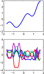
We next tested our model on a toy regression problem. A deep regression problem is similar to the unsupervised learning problem we have described, but in the uppermost layer we make observations of some set of inputs. For this simple example we created a toy data set by stacking two Gaussian processes as follows: the first Gaussian process employed a covariance function which was the sum of a linear and an quadratic exponential kernel and received as input an equally spaced vector of points. We generated -dimensional samples from the first GP and used them as input for the second GP, which employed a quadratic exponential kernel. Finally, we generated -dimensional samples with the second GP, thus overall simulating a warped process. The final data set was created by simply ignoring the intermediate layer (the samples from the first GP) and presenting to the tested methods only the continuous equally spaced input given to the first GP and the output of the second GP. To make the data set more challenging, we randomly selected only datapoints for the training set and left the rest for the test set.
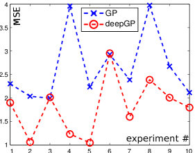
Figure 3 nicely illustrates the effects of sampling through two GP models, nonstationarity and long range correlations across the input space become prevalent. A data set of this form would be challenging for traditional approaches because of these long range correlations. Another way of thinking of data like this is as a nonlinear warping of the input space to the GP. Because this type of deep GP only contains one hidden layer, it is identical to the model developed by (Damianou et al., 2011) (where the input given at the top layer of their model was a time vector, but their code is trivially generalized). The additional contribution in this paper will be to provide a more complex deep hierarchy, but still learn the underlying representation correctly. To this end we applied a standard GP (1 layer less than the actual process that generated the data) and a deep GP with two hidden layers (1 layer more than the actual generating process). We repeated our experiment 10 times, each time obtaining different samples from the simulated warped process and different random training splits. Our results show that the deep GP predicted better the unseen data, as can be seen in figure 33. The results, therefore, suggest that our deep model can at the same time be flexible enough to model difficult data as well as robust, when modelling data that is less complex than that representable by the hierarchy. We assign these characteristics to the Bayesian learning approach that deals with capacity control automatically.
4.2 Modeling human motion
For our first demonstration on real data we recreate a motion capture data experiment from Lawrence and Moore (2007). They used data from the CMU MOCAP database representing two subjects walking towards each other and performing a ‘high-five’. The data contains 78 frames of motion and each character has 62 dimensions, leading to 124 dimensions in total (i.e. more dimensions than data). To account for the correlated motions of the subjects we applied our method with a two-level hierarchy where the two observation sets were taken to be conditionally independent given their parent latent layer. In the layer closest to the data we associated each GP-LVM with a different set of ARD parameters, allowing the layer above to be used in different ways for each character. In this approach we are inspired by the shared GP-LVM structure of Damianou et al. (2012) which is designed to model loosely correlated data sets within the same model. The end result was that we obtained three optimised sets of ARD parameters: one for each modality of the bottom layer (fig. 44), and one for the top node (fig. 44). Our model discovered a common subspace in the intermediate layer, since for dimensions and both ARD sets have a non-zero value. This is expected, as the two subjects perform very similar motions with opposite directions. The ARD weights are also a means of automatically selecting the dimensionality of each layer and subspace. This kind of modelling is impossible for a MAP method like (Lawrence and Moore, 2007) which requires the exact latent structure to be given a priori. The full latent space learned by the aforementioned MAP method is plotted in figure 5 (d,e,f), where fig. (d) corresponds to the top latent space and each of the other two encodes information for each of the two interacting subjects. Our method is not constrained to two dimensional spaces, so for comparison we plot two-dimensional projections of the dominant dimensions of each subspace in figure 5 (a,b,c). The similarity of the latent spaces is obvious. In contrast to Lawrence and Moore (2007), we did not have to constrain the latent space with dynamics in order to obtain results of good quality.
Further, we can sample from these spaces to see what kind of information they encode. Indeed, we observed that the top layer generates outputs which correspond to different variations of the whole sequence, while when sampling from the first layer we obtain outputs which only differ in a small subset of the output dimensions, e.g. those corresponding to the subject’s hand.


4.3 Deep learning of digit images
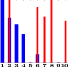
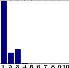
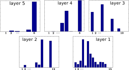
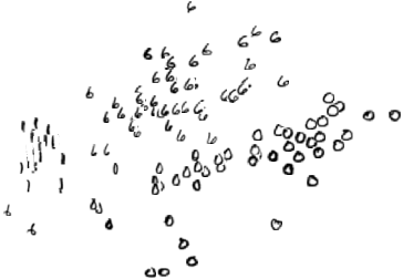
Our final experiment demonstrates the ability of our model to learn latent features of increasing abstraction and we demonstrate the usefulness of an analytic bound on the model evidence as a means of evaluating the quality of the model fit for different choices of the overall depth of the hierarchy. Many deep learning approaches are applied to large digit data sets such as MNIST. Our specific intention is to explore the utility of deep hierarchies when the digit data set is small. We subsampled a data set consisting of examples for each of the digits taken from the USPS handwritten digit database. Each digit is represented as an image in pixels. We experimented with deep GP models of depth ranging from (equivalent to Bayesian GP-LVM) to hidden layers and evaluated each model by measuring the nearest neighbour error in the latent features discovered in each hierarchy. We found that the lower bound on the model evidence increased with the number of layers as did the quality of the model in terms of nearest neighbour errors 666As parameters increase linearly in the deep GP with latent units, we also considered the Bayesian Information Criterion, but we found that it had no effect on the ranking of model quality.. Indeed, the single-layer model made mistakes even though it automatically decided to use latent dimensions and the quality of the trained models was increasing with the number of hidden layers. Finally, only one point had a nearest neighbour of a different class in the dimensional top level’s feature space of a model with depth . A projection of this space is plotted in fig.7. The ARD weights for this model are depicted in fig. 6.
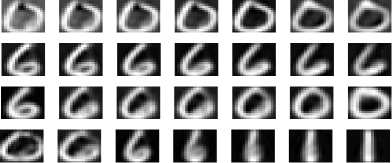
Our final goal is to demonstrate that, as we rise in the hierarchy, features of increasing abstraction are accounted for. To this end, we generated outputs by sampling from each hidden layer. The samples are shown in figure 8. There, it can be seen that the lower levels encode local features whereas the higher ones encode more abstract information.
5 Discussion and future work
We have introduced a framework for efficient Bayesian training of hierarchical Gaussian process mappings. Our approach approximately marginalises out the latent space, thus allowing for automatic structure discovery in the hierarchy. The method was able to successfully learn a hierarchy of features which describe natural human motion and the pixels of handwritten digits. Our variational lower bound selected a deep hierarchical representation for handwritten digits even though the data in our experiment was relatively scarce (150 data points). We gave persuasive evidence that deep GP models are powerful enough to encode abstract information even for smaller data sets. Further exploration could include testing the model on other inference tasks, such as class conditional density estimation to further validate the ideas. Our method can also be used to improve existing deep algorithms, something which we plan to further investigate by incorporating ideas from past approaches. Indeed, previous efforts to combine GPs with deep structures were successful at unsupervised pre-training (Erhan et al., 2010) or guiding (Snoek et al., 2012) of traditional deep models.
Although the experiments presented here considered only up to 5 layers in the hierarchy, the methodology is directly applicable to deeper architectures, with which we intend to experiment in the future. The marginalisation of the latent space allows for such an expansion with simultaneous regularisation. The variational lower bound allows us to make a principled choice between models trained using different initializations and with different numbers of layers.
The deep hierarchy we have proposed can also be used with inputs governing the top layer of the hierarchy, leading to a powerful model for regression based on Gaussian processes, but which is not itself a Gaussian process. In the future, we wish to test this model for applications in multitask learning (where intermediate layers could learn representations shared across the tasks) and in modelling nonstationary data or data involving jumps. These are both areas where a single layer GP struggles.
A remaining challenge is to extend our methodologies to very large data sets. A very promising approach would be to apply stochastic variational inference (Hoffman et al., 2012). In a recent workshop publication Hensman and Lawrence (2012) have shown that the standard variational GP and Bayesian GP-LVM can be made to fit within this formalism. The next step for deep GPs will be to incorporate these large scale variational learning algorithms.
Acknowledgements
Research was supported by the University of Sheffield Moody endowment fund and the Greek State Scholarships Foundation (IKY).
References
- Bengio [2009] Y. Bengio. Learning Deep Architectures for AI. Found. Trends Mach. Learn., 2(1):1–127, Jan. 2009. ISSN 1935-8237. doi: 10.1561/2200000006.
- Bengio et al. [2012] Y. Bengio, A. C. Courville, and P. Vincent. Unsupervised feature learning and deep learning: A review and new perspectives. CoRR, abs/1206.5538, 2012.
- Damianou and Lawrence [2012] A. C. Damianou and N. D. Lawrence. Deep Gaussian processes. NIPS workshop on Deep Learning and Unsupervised Feature Learning (arXiv:1211.0358v1), 2012.
- Damianou et al. [2011] A. C. Damianou, M. Titsias, and N. D. Lawrence. Variational Gaussian process dynamical systems. In J. Shawe-Taylor, R. Zemel, P. Bartlett, F. Pereira, and K. Weinberger, editors, Advances in Neural Information Processing Systems 24, pages 2510–2518. 2011.
- Damianou et al. [2012] A. C. Damianou, C. H. Ek, M. K. Titsias, and N. D. Lawrence. Manifold relevance determination. In J. Langford and J. Pineau, editors, Proceedings of the International Conference in Machine Learning, volume 29, San Francisco, CA, 2012. Morgan Kauffman.
- Durrande et al. [2011] N. Durrande, D. Ginsbourger, and O. Roustant. Additive kernels for Gaussian process modeling. ArXiv e-prints 1103.4023, 2011.
- Erhan et al. [2010] D. Erhan, Y. Bengio, A. Courville, P.-A. Manzagol, P. Vincent, and S. Bengio. Why does unsupervised pre-training help deep learning? J. Mach. Learn. Res., 11:625–660, Mar. 2010. ISSN 1532-4435.
- Gönen and Alpaydin [2011] M. Gönen and E. Alpaydin. Multiple kernel learning algorithms. J. Mach. Learn. Res., 12:2211–2268, Jul 2011. ISSN 1532-4435.
- Hensman and Lawrence [2012] J. Hensman and N. Lawrence. Gaussian processes for big data through stochastic variational inference. NIPS workshop on Big Learning, 2012.
- Hinton [2010] G. Hinton. A Practical Guide to Training Restricted Boltzmann Machines. Technical report, 2010.
- Hinton [1999] G. E. Hinton. Training products of experts by maximizing contrastive likelihood. Technical report, Tech. Rep., Gatsby Computational Neuroscience Unit, 1999.
- Hinton and Osindero [2006] G. E. Hinton and S. Osindero. A fast learning algorithm for deep belief nets. Neural Computation, 18:2006, 2006.
- Hinton and Salakhutdinov [2006] G. E. Hinton and R. R. Salakhutdinov. Reducing the dimensionality of data with neural networks. Science, 303(5786):504–507, 2006.
- Hoffman et al. [2012] M. Hoffman, D. Blei, C. Wang, and J. Paisley. Stochastic variational inference. ArXiv e-prints 1206.7051, 2012.
- Lawrence [2004] N. D. Lawrence. Gaussian process latent variable models for visualisation of high dimensional data. In In NIPS, page 2004, 2004.
- Lawrence [2005] N. D. Lawrence. Probabilistic non-linear principal component analysis with Gaussian process latent variable models. Journal of Machine Learning Research, 6:1783–1816, 11 2005.
- Lawrence and Moore [2007] N. D. Lawrence and A. J. Moore. Hierarchical Gaussian process latent variable models. In Z. Ghahramani, editor, Proceedings of the International Conference in Machine Learning, volume 24, pages 481–488. Omnipress, 2007. ISBN 1-59593-793-3.
- Neal [1996] R. M. Neal. Bayesian Learning for Neural Networks. Springer, 1996. Lecture Notes in Statistics 118.
- Rasmussen and Williams [2006] C. E. Rasmussen and C. K. I. Williams. Gaussian Processes for Machine Learning. Cambridge, MA, 2006. ISBN 0-262-18253-X.
- Salakhutdinov and Murray [2008] R. Salakhutdinov and I. Murray. On the quantitative analysis of deep belief networks. In Proceedings of the International Conference on Machine Learning, volume 25, 2008.
- Snelson et al. [2004] E. Snelson, C. E. Rasmussen, and Z. Ghahramani. Warped Gaussian processes. In S. Thrun, L. Saul, and B. Schölkopf, editors, Advances in Neural Information Processing Systems 16. MIT Press, Cambridge, MA, 2004.
- Snoek et al. [2012] J. Snoek, R. P. Adams, and H. Larochelle. On nonparametric guidance for learning autoencoder representations. In Fifteenth International Conference on Artificial Intelligence and Statistics (AISTATS), 2012.
- Tenenbaum et al. [2000] J. B. Tenenbaum, V. de Silva, and J. C. Langford. A global geometric framework for nonlinear dimensionality reduction. Science, 290(5500):2319–2323, 2000. doi: 10.1126/science.290.5500.2319.
- Tenenbaum et al. [2006] J. B. Tenenbaum, C. Kemp, and P. Shafto. Theory-based bayesian models of inductive learning and reasoning. In Trends in Cognitive Sciences, pages 309–318, 2006.
- Titsias [2009] M. Titsias. Variational learning of inducing variables in sparse Gaussian processes. JMLR W&CP, 5:567–574, 2009.
- Titsias and Lawrence [2010] M. K. Titsias and N. D. Lawrence. Bayesian Gaussian process latent variable model. In Y. W. Teh and D. M. Titterington, editors, Proceedings of the Thirteenth International Workshop on Artificial Intelligence and Statistics, volume 9, pages 844–851, Chia Laguna Resort, Sardinia, Italy, 13-16 May 2010. JMLR W&CP 9.
- Wilson et al. [2012] A. G. Wilson, D. A. Knowles, and Z. Ghahramani. Gaussian process regression networks. In J. Langford and J. Pineau, editors, Proceedings of the 29th International Conference on Machine Learning (ICML), Edinburgh, June 2012. Omnipress.