The SDSS-III Baryon Oscillation Spectroscopic Survey:
The Quasar Luminosity Function from Data Release Nine

Abstract

We present a new measurement of the optical Quasar Luminosity Function (QLF), using data from the Sloan Digital Sky Survey-III: Baryon Oscillation Spectroscopic Survey (SDSS-III: BOSS). From the SDSS-III Data Release Nine (DR9), we select a uniform sample of 22,301 $i\lesssim 21.8$ quasars over an area of 2236 deg² with confirmed spectroscopic redshifts between $2.2<z<3.5$, filling in a key part of the luminosity-redshift plane for optical quasar studies. We derive the completeness of the survey through simulated quasar photometry, and check this completeness estimate using a sample of quasars selected by their photometric variability within the BOSS footprint. We investigate the level of systematics associated with our quasar sample using the simulations, in the process generating color-redshift relations and a new quasar $k$-correction. We probe the faint end of the QLF to $M_{i}(z=2.2)\approx-24.5$ and see a clear break in the QLF at all redshifts up to $z=3.5$. We find that a log-linear relation (in $\log\Phi^{*}-M^{*}$) for a luminosity and density evolution (LEDE) model adequately describes our data within the range $2.2<z<3.5$; across this interval the break luminosity increases by a factor of $\sim$2.3 while $\Phi^{*}$ declines by a factor of $\sim$6. At $z\lesssim 2.2$ our data is reasonably well fit by a pure luminosity evolution (PLE) model. We see only a weak signature of “AGN downsizing”, in line with recent studies of the hard X-ray luminosity function. We compare our measured QLF to a number of theoretical models and find that models making a variety of assumptions about quasar triggering and halo occupation can fit our data over a wide range of redshifts and luminosities.

1. Introduction

Quasars, i.e. luminous active galactic nuclei (AGN), represent a fascinating and unique population of objects at the intersection of cosmology and astrophysics. The cosmological evolution of the quasar luminosity function (QLF) has been of interest since quasars were first identified a half-century ago (Sandage, 1961; Hazard et al., 1963; Schmidt, 1963; Oke, 1963; Greenstein & Matthews, 1963; Burbidge, 1967).

Measuring the QLF, and its evolution with redshift, is important for several reasons. It is generally believed that present-day supermassive black holes (SMBHs) gained most of their mass via gas accretion during an active nuclear phase, potentially at quasar luminosities ($L_{\rm Bol}\gtrsim 10^{45}$ erg s^-1; Salpeter, 1964; Zel’dovich & Novikov, 1965; Lynden-Bell, 1969; Soltan, 1982), so an accurate description of the QLF allows us to place constraints on the formation history of supermassive black holes (e.g., Rees, 1984; Madau & Rees, 2001; Volonteri et al., 2003; Volonteri & Rees, 2006; Netzer & Trakhtenbrot, 2007; Haiman, 2012) and to map the black hole accretion history of the Universe via the black hole mass function (Shankar et al., 2009, 2010; Shen, 2009; Shen & Kelly, 2012), as well as constrain the effect of black hole spin on the central engine (Volonteri et al., 2005; Fanidakis et al., 2011).

Measurements of the QLF also place constraints on the intensities and nature of various cosmic backgrounds, including the buildup of the cosmic X-ray (Shanks et al., 1991; Comastri et al., 1995; Ueda et al., 2003; Brandt & Hasinger, 2005; Hickox & Markevitch, 2006), ultraviolet (Henry, 1991) and infrared (IR) (Hauser & Dwek, 2001; Dole et al., 2006) backgrounds. Knowledge of the UV background is relevant for calculations that involve the contribution of quasar UV photons to the epoch of H reionization (e.g., Fan et al., 2006) at $z\gtrsim 6$. At lower ($z\lesssim 6$) redshift, quasars contribute towards a fraction of the ionizing photons that keep most of the H ionized, allowing studies of the Ly-$\alpha$ forest (Ly$\alpha$F; e.g. Lynds, 1971; Meiksin, 2009). Helium reionization (He II$\rightarrow$He III) can be measured by its effect on the Ly$\alpha$F (Jakobsen et al., 1994; Reimers et al., 1997; Smette et al., 2002; Reimers et al., 2005; Syphers et al., 2011; Worseck et al., 2011). This second epoch of reionization occurs at $z\sim 3$, and may be driven by UV photons from quasars, so an accurate determination of the QLF at this epoch is a key consistency check on the He reionization measurements.

Furthermore, the co-evolution of galaxies and AGN is a crucial ingredient in, and test of, modern theories of galaxy formation. The energy feedback from AGN is thought to impact their host galaxies, and thus influencing their present-day properties (e.g., Cattaneo et al., 2009; Fabian, 2012). Observations of the evolution of quasar properties over cosmic time can inform such models and therefore our understanding of the galaxy-black hole connection.

Recent large quasar surveys have allowed us to study the properties of the quasar population with unprecedented statistical precision. The number of known quasars has increased nearly 100-fold since the late 1990s, (for photometrically identified quasars, see Richards et al., 2009) and since that time, there has been a large effort to measure the QLF in the UV/optical (Boyle et al., 2000; Fan et al., 2001; Wolf et al., 2003; Hunt et al., 2004; Fan et al., 2004; Croom et al., 2004; Hao et al., 2005; Richards et al., 2005, 2006b; Fan et al., 2006; Jiang et al., 2006; Fontanot et al., 2007; Bongiorno et al., 2007; Reyes et al., 2008; Jiang et al., 2008, 2009; Croom et al., 2009a; Glikman et al., 2010; Willott et al., 2010; Glikman et al., 2011; Ikeda et al., 2011, 2012; Masters et al., 2012), mid-infrared (Brown et al., 2006; Siana et al., 2008; Assef et al., 2011) and the soft and hard X-ray (Cowie et al., 2003; Ueda et al., 2003; Hasinger et al., 2005; Barger et al., 2005; Silverman et al., 2005, 2008; Aird et al., 2008; Treister et al., 2009; Aird et al., 2010; Fiore et al., 2012). An overview of recent determinations of the optical QLF is given in Table LABEL:tab:previous_surveys.

Table 1Selected optical quasar luminosity function measurements.
^aCosmic Evolution Survey (Scoville et al., 2007b).
^bNo Type-1 quasars were identified, though a low-luminosity $z\sim 5.07$ Type-2 quasar was discovered.
^cNOAO Deep Wide-Field Survey (Jannuzi & Dey, 1999) and the Deep Lens Survey (Wittman et al., 2002).
^dSDSS Faint Quasar Survey.
^eThe “boss21” area on the SDSS Stripe 82 field.
^f2dF-SDSS LRG And QSO Survey (Croom et al., 2009b).
^gPhotometric sample from SDSS; spectroscopic confirmation from SDSS and other telescopes.
^hCanada-France High-$z$ Quasar Survey (Willott et al., 2009)
ⁱ2dF Quasar Redshift Survey (Croom et al., 2004).
^jFrom our “uniform” sample defined in Section 2.3
^kFrom a catalog of $>$1,000,000 photometrically classified quasar candidates.

Survey	Area (deg2)	NQ	Magnitude Range	$z$-range	Reference
GOODS(+SDSS)	0.1+(4200)	13(+656)	$22.25<z_{850}<25.25$	$3.5<z<5.2$	Fontanot et al. (2007)
VVDS	0.62	130	$17.5<I_{\rm AB}<24.0$	$0<z<5$	Bongiorno et al. (2007)
COMBO-17	0.8	192	$R<24$	$1.2<z<4.8$	Wolf et al. (2003)
COSMOSa	1.64	8	$22<i^{\prime}<24$	$3.7\lesssim z\lesssim 4.7$	Ikeda et al. (2011)
COSMOS	1.64	b0	$22<i^{\prime}<24$	$4.5\lesssim z\lesssim 5.5$	Ikeda et al. (2012)
COSMOS	1.64	155	$16\leq I_{\rm AB}\leq 25$	$3<z<5$	Masters et al. (2012)
NDWFS+DFSc	4	24	$R\leq 24$	$3.7<z<5.1$	Glikman et al. (2011)
SFQSd	4	414	$g<22.5$	$z<5$	Jiang et al. (2006)
BOSSe+MMT	14.5+3.92	1 877	$g\lesssim 23$	$0.7<z<4.0$	Palanque-Delabrouille et al. (2012)
2SLAQf	105	5 645	$18.00<g<21.85$	$z\leq 2.1$	Richards et al. (2005)
SDSSg	182	39	$i\leq 20$	$3.6<z<5.0$	Fan et al. (2001)
SDSS+2SLAQ	192	10 637	$18.00<g<21.85$	$0.4<z<2.6$	Croom et al. (2009a)
SDSS Main+Deep	195	6	$z_{\rm AB}<21.80$	$z\sim 6$	Jiang et al. (2009)
BOSS Stripe 82	220	5 476	$i>$18.0 and $g<$22.3	2.2$<z<$3.5	Palanque-Delabrouille et al. (2011)
CFHQSh	500	19	$z^{\prime}<22.63$	$5.74<z<6.42.$	Willott et al. (2010)
2QZi	700	23 338	$18.25<b_{\rm J}<20.85$	$0.4<z<2.1$	Boyle et al. (2000); Croom et al. (2004)
SDSS DR3	1622	15 343	$i\leq 19.1$ and $i\leq 20.2$	$0.3<z<5.0$	Richards et al. (2006b)
BOSS DR9	2236	j23 201	$g<$22.00 or $r<$21.85	2.2$<z<$3.5	this paper
SDSS DR7	6248	57 959	$i\leq 19.1$ and $i\leq 20.2$	$0.3<z<5.0$	Shen & Kelly (2012)
SDSS Type 2	6293	887	$L_{\rm OIII}\geq 10^{8.3}L_{\odot}$	$z<0.83$	Reyes et al. (2008)
SDSS DR6k	8417	$\gtrsim\hbox{850,000}$	$i<21.3$	$z\sim 2$ and $z\sim 4.25$	Richards et al. (2009)

Quasar number density evolves strongly with redshift (Schmidt, 1970; Osmer, 1982; Schmidt et al., 1995; Fan et al., 2001; Richards et al., 2006b; Croom et al., 2009b), and one of the key goals of quasar studies is to understand what drives this strong evolution. A caveat here is that the evolution of the optical QLF is a composite of intrinsic quasar evolution and the evolution of the obscuring medium in quasar hosts. In this study, we concentrate on the unobscured quasar population, defined as objects that were selected via their UV/optical rest-frame continuum and the presence of broad, $\gtrsim$1000 ${\rm~{}km~{}s}^{-1}$, emission lines. We leave investigations of the obscured AGN population to other studies, e.g., in the mid-infrared (e.g., Lacy et al., 2004; Richards et al., 2006a; Stern et al., 2012; Yan et al., 2012), and X-ray (Tueller et al., 2010; Luo et al., 2011; Corral et al., 2011; Brightman & Ueda, 2012; Lehmer et al., 2012). As the QLF is observed to have a broken power-law form, it is necessary to probe below the luminosity at which the power-law breaks in order to distinguish luminosity evolution (where the luminosity of AGN changes with time, but their number density remains constant) from density evolution (where the number density of AGN changes, but the luminosities of individual objects remains constant), or a combination of the two.

The QLF is defined as the number density of quasars per unit luminosity. It is often described by a double power-law (Boyle et al., 2000; Croom et al., 2004; Richards et al., 2006b, hereafter, R06) of the form

$$\Phi(L,z)=\frac{\phi_{*}^{(L)}}{(L/L^{*})^{\alpha}+(L/L^{*})^{\beta}}\ \,$$ (1)

with a characteristic, or break, luminosity $L_{*}$. An alternative definition of this form of the QLF gives the number density of quasars per unit magnitude,

$$\Phi(M,z)=\frac{\phi_{*}^{(M)}}{10^{0.4{(\alpha+1)[M-M^{*}(z)]}}+10^{0.4{(\beta+1)[M-M^{*}(z)]}}}$$ (2)

The dimensions of $\Phi$ differ in the two conventions. We have followed R06 such that $\alpha$ describes the faint end QLF slope, and $\beta$ the bright end slope. The $\alpha$/$\beta$ convention in some other works (e.g., Croom et al., 2009a) is in the opposite sense from our definition. Evolution of the QLF can be encoded in the redshift dependence of the break luminosity, $\phi_{*}$, and also potentially in the evolution of the power-law slopes.

Boyle et al. (2000) and Croom et al. (2004) found that the QLF measured in the 2dF Quasar Redshift Survey (2QZ, Croom et al., 2004) was well fit by a pure luminosity evolution model where $\Phi_{*}^{(M)}$ was constant but $M_{*}$ evolved with redshift. In this model, $M_{*}$ changed from $\approx-26.0$ to $\approx-22.0$ between $z\sim 2.5$ and $z\sim 0$. However, this paradigm is challenged using recent, deeper data. Croom et al. (2009a) measured the optical quasar luminosity function at $z\leq 2.6$ from the combination of the 2dF-SDSS LRG And QSO survey (2SLAQ; Croom et al., 2009b), which probes down to a magnitude limit of $g=21.85$, and the SDSS-I/II Quasar survey (Richards et al., 2002; Schneider et al., 2010) to $i=19.1$ ($z\lesssim 3$) and $i=20.2$ ($z\gtrsim 3$). Here, the double power-law form with pure luminosity evolution provides a reasonable fit to the observed QLF from low $z$ up to $z\simeq 2$, but it appears to break down at higher redshift. However, the 2SLAQ sample has few objects above $z\sim 2$, and SDSS does not probe down to $L_{*}$ at higher redshifts, making it difficult to constrain the faint end of the QLF at high $z$.

At $z\gtrsim 2$, the constraints on the QLF are less clear-cut, as the selection of luminous quasars becomes less efficient. This situation arises because the broad-band colors of $z\approx 2.7$ and $z\approx 3.5$ quasars are very similar to those of A and F stars (Fan, 1999; Fan et al., 2001; Richards et al., 2002; Ross et al., 2012) in the Sloan Digital Sky Survey color system (Fukugita et al., 1996). Although we have good constraining power at the bright end at $z>2$, (e.g. Richards et al., 2006b; Jiang et al., 2009), there is uncertainty in the form, and evolution of the QLF at $z>2$, especially at the faint end. The redshift range $z\sim 2-3$ is of particular importance since the luminous quasar number density peaks here; this is often referred to as the “quasar epoch” (Osmer, 1982; Warren et al., 1994; Schmidt et al., 1995; Fan et al., 2001; Richards et al., 2006b; Croom et al., 2009a).

For our study, we use data from the SDSS-III: Baryon Oscillation Spectroscopic Survey (BOSS; Dawson et al., 2012) that is specifically designed to target faint, $g\lesssim 22$, quasars in the redshift range $z=2.2-3.5$ (Ross et al., 2012). The first two phases of the SDSS (“SDSS-I/II”, hereafter simply SDSS; York et al., 2000) have been completed (Abazajian et al., 2009), with a sample of $\approx$100,000 spectroscopically confirmed quasars at $0<z\lesssim 5$ (Schneider et al., 2010). The third incarnation of the Sloan Digital Sky Survey (SDSS-III; Eisenstein et al., 2011) is taking spectra of 150,000 $z>2.2$ quasars as part of the BOSS. The main scientific motivation for the SDSS-III BOSS Quasar survey is to measure the baryon acoustic oscillation feature (BAO) in the Lyman-$\alpha$ forest (Ly$\alpha$F; Slosar et al., 2011). This sample is designed to select quasars with $2.2<z<3.5$, and will have an order of magnitude more objects at $z>2$ than SDSS, sampling the quasar luminosity function $\sim 2$ magnitudes deeper at each redshift. Combining the BOSS and SDSS observations gives a dynamic range of $\sim$5 magnitudes at a given redshift, and a primary motivation for our study is to extend the work presented in Richards et al. (2006b), both in dynamic range in luminosity, and concentrating on the redshift range $z=2.2-3.5$, where the original SDSS selection was sparse-sampled in an attempt to minimize the contamination by stars (Richards et al., 2002).

In this paper we present the optical quasar luminosity function (QLF) from the first two years of BOSS spectroscopy, data included in SDSS Data Release Nine (DR9; Ahn et al., 2012). We use data from the 3671 deg² observed over the DR9 footprint, and supplement this with deeper data over a smaller area (14.6 deg²), in order to probe the redshift range $0.7<z<2.2$, also observed as part of the BOSS (Table LABEL:tab:previous_surveys; Palanque-Delabrouille et al., 2012). Table LABEL:tab:previous_surveys places the BOSS DR9 survey in context as a wide-field, medium-depth survey, and we will return to the surveys that match BOSS in redshift.

The outline of this paper is as follows. In Section 2 we describe our data sets, which includes both color and variability selected AGN samples. In Section 3, we qualitatively compare our different quasar samples, and quantify our selection function using both empirical data, and new, updated template quasar spectra. In Section 4 we present the SDSS+BOSS quasar number counts and a new quasar $k$-correction based on our simulations. In Section 5, we present the combined SDSS+BOSS QLF, sampling the range $-24.5<M_{i}<-30$ in absolute magnitude across redshifts $0.7<z<3.5$ and compare to previous measurements. In Section 6, various models of the double-power law form are fit to our data, we compare our results to recent theoretical predictions in the literature, and place our new results in a broader context. We present our conclusions in Section 7. In Appendix A we investigate further the selection function models introduced in Section 3 and in Appendix B provide tables of our measured QLFs. For direct comparison with, and extension of, R06, we assume a flat cosmology with $\Omega_{\Lambda}$=0.70 and $H_{0}=70~{}\;h^{-1}~{}{\rm Mpc}$. Our magnitudes are based on the AB zero-point system (Oke & Gunn, 1983) and are PSF magnitudes (Stoughton et al., 2002), corrected for Galactic extinction following Schlegel et al. (1998). Absolute magnitudes ($M$) are determined using luminosity distances for this cosmology (Peebles, 1980, 1993; Hogg et al., 2002; Wright, 2006).

Figure 1.— The sky coverage of the SDSS-III: BOSS DR9 quasar dataset (colored regions) overlaid on the final expected footprint of BOSS (gray). These areas are 3671 and 10 269 deg², respectively. The upper panel shows the coverage in the NGC, and the lower one is the SGC. Each sector (covered by a unique combination of spectroscopic tiles) is colored according to the fraction of quasar targets, selected with the uniform XDQSO algorithm, which have successful redshifts. The sectors which contribute data to the QLF analysis have $>85\%$ spectroscopic completeness (yellow-orange-red regions). This area is 2236 deg². The Stripe 82 field runs from $-43^{\circ}<$ R.A. $<45^{\circ}$ at Decl.$=\pm 1.25^{\circ}$ and generally has $f_{\rm sc}<0.85$ (where $f_{\rm sc}$ is defined in Sec. 3.1.4). However, since Stripe 82 had quasar targets that were variability selected (see Sec. 2.4), the true number of quasars in this field is actually very high.

2. Data

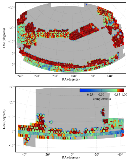
We use imaging data that are part of Data Release Eight (DR8; Aihara et al., 2011) in order to select spectroscopic targets that form the Data Release Nine (Ahn et al., 2012) dataset. Ross et al. (2012) describes the BOSS quasar target selection algorithms used to identify objects for spectroscopy. In summary, we use the subset of the DR9 data that employs the “Extreme Deconvolution” (XDQSO) algorithm of Bovy et al. (2011) to select quasars based on their optical fluxes and colors to define a uniform sample. The XDQSO procedure is supplemented by a selection using optical variability, where we have repeat imaging data within the DR8 footprint. The DR9 data are the first two years of BOSS spectroscopic data, and the full DR9 Quasar Catalog (DR9Q) is detailed in Pâris et al. (2012). Fig 1 shows the sky coverage of the DR9 quasar dataset. However, the XDQSO selection was not implemented in the first year, leading to effects on completeness that we will address below in order to perform a QLF measurement.

2.1. Imaging and Target Selection

The SDSS-III:BOSS uses the imaging data gathered by a dedicated 2.5m wide-field telescope (Gunn et al., 2006), which collected light for a camera with 30 2k$\times$2k CCDs (Gunn et al., 1998) over five broad bands - ugriz (Fukugita et al., 1996) - in order to image 14,555 unique deg² of the sky. This area includes 7,500 deg² in the North Galactic Cap (NGC) and 3,100 deg² in the South Galactic Cap (SGC). The imaging data are taken on dark photometric nights of good seeing (Hogg et al., 2001) and are calibrated photometrically (Smith et al., 2002; Ivezić et al., 2004; Tucker et al., 2006; Padmanabhan et al., 2008), and astrometrically (Pier et al., 2003) before object parameters are measured (Lupton et al., 2001; Stoughton et al., 2002).

Using the imaging data, BOSS quasar target candidates are selected for spectroscopic observation based on their fluxes and colors in SDSS bands. However, selection of quasars for BOSS spectroscopy is complicated by two facts: (i) The optical colors of $z\sim 2.7$ quasars resemble faint A and F stars (Fan, 1999; Richards et al., 2001b; Ross et al., 2012) and (ii) to maximize the number density of quasars for Ly$\alpha$F cosmology, we are required to work close to the magnitude limit of the (single-epoch) imaging data, leading to larger photometric errors, expansion of the stellar locus and higher stellar contamination. All objects classified as point-like and having magnitudes of $g\leq 22$ or $r<21.85$ are passed to the quasar target selection code.

As was the case for the original SDSS Quasar survey, radio data was used to select quasars. Specifically, optical stellar objects with $g\leq 22$ or $r\leq 21.85$ which have matches within 1^′′ to radio sources apparent in the Faint Radio Sources at Twenty cm (FIRST) survey (Becker et al., 1995) are considered as potential quasar targets, irrespective of their radio morphology. Approximately 2% of targets, and $\approx$1.3% of our uniform quasar sample (defined in § 2.3 below), satisfy the radio selection criteria.

As the main science goal of the BOSS quasar sample is to probe the foreground hydrogen in the IGM, priority was placed on maximizing the surface density of $z>2$ quasars (McDonald & Eisenstein, 2007; McQuinn & White, 2011), rather than creating a homogeneous dataset. The target selection is consequently a complicated heterogenous combination of several methods (Ross et al., 2012). However, a uniform subsample (called “CORE” in Ross et al., 2012) was defined to allow statistical studies of quasar demographics to be performed. The spectroscopic observations, and creation of this uniform subset of objects, are described in the next two sections.

2.2. Spectroscopy

The BOSS spectrographs and their SDSS predecessors are described in detail by Smee et al. (2012). In brief, there are two double-armed spectrographs that are significantly upgraded from those used by SDSS-I/II. They cover the wavelength range $3600\,$Å to $10,400\,$Å with a resolving power of 1500 to 2600 (Smee et al., 2012). In addition, the throughputs have been increased with new CCDs, gratings, and improved optical elements, and the 640-fibre cartridges with $3"$ apertures have been replaced with 1000-fibre cartridges with $2"$ apertures. Each observation is performed in a series of 900-second exposures, integrating until a minimum signal-to-noise ratio is achieved at a fiducial magnitude for the given spectroscopic plate (Dawson et al., 2012).

Once target selection is completed, the spectroscopic targets are assigned to tiles of diameter $3^{\circ}$ using an algorithm that is adaptive to the density of targets on the sky (Blanton et al., 2003). Of the 1000 available fibers on each tile, a maximum of 900 fibers are allocated for science targets, of which $\sim$160-200 are allocated to quasar targets, while 560-630 fibers are assigned to galaxy targets, and 20-90 to ancillary science targets (Dawson et al., 2012). Because of the 62^′′ diameter of the cladding around each optical fiber, two targets with a separation smaller than that angle cannot both be observed on a given spectroscopic plate, and different classes of targets are assigned priorities when such a collision arises. CORE quasars are assigned higher tiling priority than the galaxy targets (Appendix B of Ross et al., 2012). To cover the survey footprint without leaving gaps, adjacent tiles overlap, alleviating the fiber collisions problem somewhat. This leads to the definition of a “sector” - a region covered by a unique set of tiles (see Blanton et al., 2003; Tegmark et al., 2004; Swanson et al., 2008; White et al., 2011). As in previous SDSS analyses, we work on a sector-by-sector basis to define our various completenessess.

Figure 2.— Quasar $N(z)$ redshift distributions. The dotted red histogram shows the redshift distribution for the full SDSS-III: BOSS DR9 quasar dataset, while the solid red line shows those objects uniformly selected by the “XDQSO” method across $2.2<z<3.5$. The black histogram is the final distribution from the DR7Q catalog of Schneider et al. (2010).

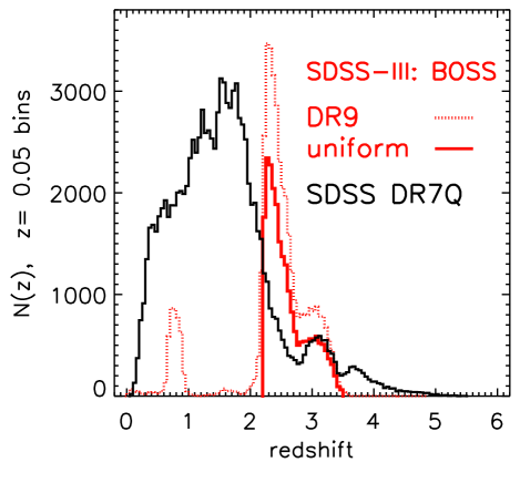
The DR9 footprint is 3 671 deg², and is given in Fig. 1. In total, we obtained 182 973 spectra of objects that were selected as BOSS quasar targets, and Bolton et al. (2012) describes the automated spectral classification, redshift determination, and parameter measurement pipeline used for the BOSS. A total of 167 331 of these had the specPrimary flag set to 1, indicating that this was the best spectroscopic observation of an object; this cut, by definition, removes objects with duplicate spectra. As described in Adelman-McCarthy et al. (2008) and Bolton et al. (2012), each redshift is accompanied by a flag, zWarning, which is set when the automatically derived (a.k.a. pipeline) redshift and classification are not reliable; 132 290 of these objects do not have this flag set. Of these, 54 019 have pipeline redshifts between 2.2 and 3.5. A summary of these numbers is given in Table 2.

Each of the quasar target spectra has also been visually inspected, and the redshift corrected where necessary. In total there are 87 822 spectroscopically confirmed quasars in the DR9Q, while approximately half the quasar candidates were stars (Pâris et al., 2012). If there was confidence in a secure redshift from the visual inspection of the spectrum, the flag z_conf_person was set to be $\geq 3$. Most of the zWarning $\neq 0$ objects have secure redshifts after visual inspection; over 97% of the specPrimary BOSS quasar target spectra have secure redshifts (Table 2). Among these objects, 54 593 are confirmed, by visual inspection, to be at $2.2<z<3.5$. For comparison the DR7Q (Schneider et al., 2010) has 14 063 objects in this redshift range.

Description	No. of Objects
	Pipelinea	Visually
		Inspected
All DR9 boss_target1 quasar targetsb	182 973	—
specPrimary = 1	167 331	—
” and reliable redshiftc	132 290	163 128
” and $2.2<z<3.5$	54 019	54 593
XDQSO DR9 quasar targets	74 607	—
” with spectrad	63 061	—
” and reliable redshiftc	54 416	62 048
” and $2.2<z<3.5$	34 803	35 099
” and $f_{\rm sc}\geq 0.85$		23 301

Table 2Properties of the SDSS-III BOSS DR9 QLF dataset.
^aThe automated redshift determination algorithms described in Bolton et al. (2012). ^bThe DR9 quasar boss_target1 target flag is defined in Ross et al. (2012). ^cTotals include stars. ^dAll XDQSO DR9 quasar target spectra have specprimary=1 by design. The uniform sample defined in Section 2 is based upon the XDQSO selection.

2.3. DR9 Uniform Sample

We now define a uniform subsample from the parent DR9 quasar dataset. XDQSO models the distribution in SDSS flux space of stars and quasars as a function of redshift, as a sum of Gaussians convolved with photometric measurement errors, allowing the Bayesian probability that any given object is a quasar to be calculated. XDQSO is specifically trained and designed to select quasars in the redshift range $2.2<z<3.5$ down to the BOSS limiting magnitude.

XDQSO was only chosen as the algorithm to define the uniform sample after the first year of BOSS spectroscopic observations. Each object is assigned a probability, P(QSOMIDZ), that it is a quasar with $2.2<z<3.5$. Objects with P(QSOMIDZ) $>0.424$ (Bovy et al., 2011) are targeted as part of the uniform (CORE) sample. Knowing this threshold, we are able to say which targets XDQSO would have targeted in the first year of observations, many of which BOSS did obtain spectra for. There are 74 607 quasar targets selected by XDQSO over the DR9 footprint, 63 061 of which have spectroscopic observations, and of these, over half (35 099) are confirmed $2.20<z<3.50$ quasars by visual inspection (Pâris et al., 2012).

This sample of 35 099 quasars is over an order of magnitude more objects in this redshift range than in the study of Richards et al. (2006b) from DR3 (Abazajian et al., 2005). Fig. 2 shows the redshift distribution of this sample. Although we plot the full redshift range of the quasars, we do not use data from quasars which have a redshift below 2.2 or above 3.5, where the mid-$z$ XDQSO selection, by design, is quite incomplete. The BOSS DR9 uniform quasar sample has a mean (median) redshift of $\langle z\rangle=2.59$ (2.49).

This uniform dataset is our primary basis for the QLF measurement. We supplement these data with a complementary dataset, selected by photometric variability criteria.

2.4. Variability selection: Stripe 82

The $\sim$300 deg² area centered on the Celestial Equator in the Southern Galactic Cap, commonly referred to as “Stripe 82”, was imaged repeatedly by the SDSS over 10 years, generating up to 80 epochs (Abazajian et al., 2009), due in large part to the SDSS Supernova Survey (Frieman et al., 2008). These data are beneficial for quasar target selection for two reasons: (i) the improved photometry of the deeper data better defines the stellar locus (Ivezić et al., 2007) and (ii) quasars can be selected based on their variability (Sesar et al., 2007; Bramich et al., 2008; Schmidt et al., 2010; MacLeod et al., 2011; Palanque-Delabrouille et al., 2011, 2012).

Palanque-Delabrouille et al. (2011) describe the spectroscopic quasar target selection for BOSS on 220 deg² of Stripe 82 based on variability. This variability selection was designed to select quasars with $i>18.0$ and $g<22.3$ mag and redshift $z>2.15$ (Palanque-Delabrouille et al., 2011, Sec. 3.2). This dataset — which we shall refer to as the Stripe 82 (S82) data in what follows — includes $\sim$6000 $z>2$ quasars, roughly half of which would have been selected by XDQSO (as seen in Fig. 1). Since the completeness of the variability selection is only very weakly dependent on redshift (e.g., Fig. 11 of Palanque-Delabrouille et al., 2011) these data are subject to different, and arguably much weaker, selection biases than a color-based selection, as we show in Section 3.2.

R.A.	Decl.	u-band	g-band	r-band	i-band	z-band	i-band	$z_{\rm pipe}$	$z_{\rm vis}$	$f_{\rm sc}$
(J2000)	(J2000)						extinction
0.031620	0.495352	20.845$\pm$0.060	20.319$\pm$0.027	20.377$\pm$0.028	20.206$\pm$0.035	19.922$\pm$0.092	0.0527	2.260	2.254	0.4615
0.058656	1.497665	22.591$\pm$0.295	20.455$\pm$0.029	20.013$\pm$0.026	19.686$\pm$0.030	19.650$\pm$0.081	0.0509	3.228	3.228	0.8947
0.063211	0.809249	22.357$\pm$0.190	19.852$\pm$0.024	19.240$\pm$0.017	19.129$\pm$0.018	18.898$\pm$0.035	0.0585	3.028	3.028	0.8333
0.074886	0.407500	21.434$\pm$0.139	20.876$\pm$0.030	20.805$\pm$0.038	20.648$\pm$0.042	20.214$\pm$0.132	0.0540	2.282	2.281	0.4615
0.075538	1.610326	21.568$\pm$0.144	20.848$\pm$0.036	20.903$\pm$0.044	20.811$\pm$0.059	20.417$\pm$0.151	0.0485	2.400	2.400	0.8947
0.077683	3.548377	21.097$\pm$0.108	20.439$\pm$0.027	20.349$\pm$0.032	20.216$\pm$0.038	19.772$\pm$0.090	0.0563	2.237	2.238	0.7143
0.085803	3.399193	24.714$\pm$0.886	21.823$\pm$0.056	21.257$\pm$0.046	21.499$\pm$0.080	20.850$\pm$0.179	0.0569	2.904	2.903	0.7143
0.112584	3.120975	19.307$\pm$0.028	18.788$\pm$0.020	18.736$\pm$0.018	18.747$\pm$0.022	18.571$\pm$0.034	0.0451	2.353	2.343	1.0000
0.113820	1.523919	21.532$\pm$0.141	21.006$\pm$0.040	20.889$\pm$0.044	20.910$\pm$0.065	20.428$\pm$0.156	0.0500	2.589	2.589	0.8947
0.132704	1.685750	22.735$\pm$0.319	21.830$\pm$0.057	21.918$\pm$0.082	21.769$\pm$0.096	21.639$\pm$0.275	0.0476	2.526	2.526	0.8947

Table 3 The BOSS DR9 statistical quasar dataset. The first ten lines are shown here for guidance regarding its format and content. The full table is published in the electronic edition of The Astrophysical Journal. More details of the pipeline and visual inspection redshifts are documented in Bolton et al. (2012) and Pâris et al. (2012).

Figure 3.— Splitting the sample of variability selected $2.2<z<3.5$ Stripe 82 quasars into the 2 333 that are selected by the XDQSO algorithm (red) and those (3 143) that are not (blue). (Left): The distributions in the $(u-g)$ vs. $(g-r)$ color-color plane, (the stellar locus is given by the black contours); (Center): the $(g-i)$ vs. $i$-band and (Right): the resulting $N(z)$ histogram, (with all z_conf_person$\geq$3 objects indicating a secure, visually inspected, redshift) plotted by the black line.

3. Survey Completeness

To measure the QLF we must quantify the probability, $P(z,M,{\rm SED})$, of spectroscopically confirming a quasar of a given redshift $z$, absolute magnitude $M$ and Spectral Energy Distribution (SED) shape. In this section, we describe the sources of incompleteness in the sample, and our checks of our completeness corrections. Our focus in this section will be on the DR9 data; discussion of the completeness for the S82 sample can be found in Palanque-Delabrouille et al. (2011) and Ross et al. (2012).

3.1. Incompleteness Descriptions

We follow the approaches of Croom et al. (2004) and Croom et al. (2009b) to quantify four avenues of potential sample incompleteness: Morphological, Targeting, Coverage and Spectroscopic, and give descriptions of each type.

3.1.1 Morphological completeness

The input catalog to the BOSS quasar targeting algorithm is restricted to objects with stellar morphologies in the single-epoch SDSS imaging. Host galaxies of $z>2$ quasars are highly unlikely to be detected in this imaging, thus viable quasar targets should be unresolved. However, any true quasars not targeted because they are erroneously classified as resolved in the photometry will contribute to the survey incompleteness; this is referred to as morphological completeness ($f_{\rm m}$).

We checked the assumption that $z>2$ host galaxies are undetected in SDSS imaging, and tested the reliability of the star/galaxy classifier from the SDSS photometric pipeline photo (Lupton et al., 2001; Scranton et al., 2002), to the BOSS target selection magnitude limit. To do this, we compare to the Hubble Space Telescope (HST) observations of the COSMOS field (Scoville et al., 2007a), which has been observed by the SDSS imaging camera. Objects classified as extended by SDSS that are actually unresolved in the COSMOS imaging, could be true high-$z$ quasars that we fail to target in BOSS. We found that at $r\leq 21.0$, $\lesssim$3% of objects classified morphologically as galaxies by SDSS are unresolved in COSMOS; this fraction rises to $\approx$8% at $r=22.0$. We also found that all BOSS quasars at $z>2$ lying within the COSMOS field are unresolved by HST. Thus we conclude that host galaxy contribution to morphological incompleteness is minimal, and we do not account for the misclassification rate of stellar objects by photo in our QLF calculations.

3.1.2 Targeting completeness

Targeting completeness, $f_{t}$, accounts for any true quasars which are not targeted by our selection algorithm. We use the XDQSO method to select our high-$z$ quasar targets, but, as we demonstrate below, the completeness of XDQSO is a strong function of color, redshift and magnitude. Also, as we have noted, the XDQSO method was not used to select a uniform sample until the end of Year One.

The area targeted with Year One target selection was 1661 deg², although the 220 deg² of Stripe 82 was re-targeted and re-observed in Year Two. Ross et al. (2012) found that apart from over the Stripe 82 area, the fraction of objects selected by the XDQSO CORE algorithm which actually were targeted, was 87% for the DR9 footprint. This result is consistent with the numbers of XDQSO targets (74,607) that have spectra (63,074), as given in Table 2.

In Stripe 82, this fraction declines to 65.4%. This drop in targeting completeness is due to the deeper Stripe 82 photometry which eliminates many noisy stellar contaminants in the single-epoch XDQSO target list, while selecting nearly all of the true quasars selected by CORE. The high targeting completeness fraction of XDQSO in the remainder of Year One is because many of the CORE quasar targets (and consequently true quasars) were selected by other target selection methods. There are in some sense the “easiest” quasars to discover. Indeed, Bovy et al. (2011) demonstrate that XDQSO and the Likelihood method (Kirkpatrick et al., 2011), used as CORE for Year One, select similar samples.

Figure 4.— The redshift distribution for radio-selected objects (“FIRST”, blue histogram) and those that passed both the radio and XDQSO selection (“FIRST”+XD, green histogram).

3.1.3 Coverage completeness

Coverage completeness, $f_{\rm c}(\theta)$, is defined as the fraction of BOSS quasar targets that have spectroscopic observations, is quantified on a sector-by-sector basis, and is thus a function of angular position, $\theta$. The main source of coverage incompleteness is fiber collisions, i.e. fibers cannot be placed closer than 62^′′ to each other on a single plate. In Year One, the coverage completeness was $\gtrsim 90\%$, and in Year Two CORE quasars were given highest tiling priority, and $f_{\rm c}(\theta)$ is $>98$%.

3.1.4 Spectroscopic completeness

Spectroscopic completeness, $f_{s}({\rm mag},z,\theta)$, is the fraction of BOSS quasar targets with spectra, from CORE, that have reliable redshifts. With the visual inspections of all the quasar target spectra, this fraction is $>90\%$. We define a “spectro-coverage completeness” as $f_{\rm sc}=f_{\rm c}\times f_{s}$, which is the fraction of XDQSO targets that were allocated fibers, and returned a reliable spectrum. Tests showed that the computation of the QLF is only very weakly sensitive to the value of $f_{\rm sc}$, and we choose a threshold of $f_{\rm sc}=0.85$ as a good compromise between high completeness and large sample size. Sectors with $f_{\rm sc}\geq 85$% are shown in red shades in Fig. 1; we limit our LF analysis to this area. This approach tends to exclude regions that have Year One spectroscopy, leaving an area of 2236 deg². There are 23 301 quasars in this area (all with visually confirmed redshifts) and this sample is given in Table 3.

Description	No. of Objects
	Pipeline	V.I.
All Stripe 82 quasar targetsa	15 576	—
with specPrimary = 1	12 576	—
AND reliable redshifts	10 506	11 990
AND $2.20<z<3.50$	5 433	5 476
AND w/ XDQSO seln.	2 318	2 333

Table 4Properties of the Stripe 82 BOSS QLF dataset, described in Palanque-Delabrouille et al. (2011) and with data from two of the Ancillary Programs that targeted quasars due to their near-infrared colors or radio properties.

3.2. Empirical checks using Variability selected Quasars

The 220 deg² of spectroscopy across the Stripe 82 field has targets selected via their optical variability (Palanque-Delabrouille et al., 2011, and § 2.4). We concentrate on the 5 476 $2.20<z<3.50$ quasars in Stripe 82 (Table 4), including 122 quasars selected solely due to their near-infrared colors or radio properties (Dawson et al., 2012). In this area, we find a higher surface density of high-$z$ quasars, 24.9 deg^-2, than across the full DR9 dataset (14.7 deg^-2) and the XDQSO uniform sample (9.6 deg^-2). Thus, this enhanced Stripe 82 dataset is more complete and less affected by color-induced selection biases, and we will use it to measure the targeting completeness of our XDQSO uniform sample empirically.

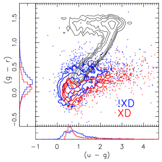
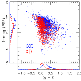
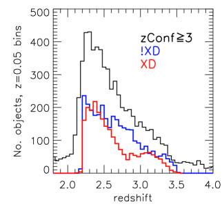
We split the sample of 5 476 visually confirmed $2.2<z<3.5$ quasars into the 2 333 that would have been selected by the XDQSO algorithm (XD) and those (3 143) that would not have been (!XD). Over 96% of the !XD sample was selected by a variability algorithm. The $(u-g)$ vs. $(g-r)$ color-color plane, their distribution in $(g-i)$ vs. $i$-band and the resulting $N(z)$ redshift histograms of these two samples are given in Fig. 3.

The difference between the two selections is apparent and consistent with that in Palanque-Delabrouille et al. (2011, their Fig. 18). The !XD sample more heavily overlaps with the stellar locus in $(u-g)$ vs. $(g-r)$, and is generally redder than the XD population in $(g-r)$. Thus, the variability selection is able to recover quasars from the stellar locus. The distribution of XD and !XD objects in the $(g-r)$ vs. $(r-i)$ color-color plane (not shown) is similar, in that the !XD population overlaps with the stellar locus, but both populations have similar distributions in the $(r-i)$ color (again in agreement with Fig.18 of Palanque-Delabrouille et al., 2011). However, the !XD population is redder in $(g-i)$ (Fig. 3, center).

The $N(z)$ histograms for the two samples are also very much in line with previous studies (e.g., Richards et al., 2006b; Palanque-Delabrouille et al., 2011). The decrement at $z\sim 2.7-2.9$ for the XD selection is due to the overlap of such objects with the stellar locus in color-space, a key issue in the original studies in SDSS.

The two samples are similar in their distributions across $z=3.0-3.3$, though at $z\approx 3.4-3.5$, there are more !XD objects, probably due to the efficient cut-off of the $z=2.2-3.5$ “mid-$z$” XDQSO selection, and the fact that at $z\sim 3.5$ quasar colors again approach the stellar locus.

Figure 5.— Color-redshift relation for BOSS quasars selected by XDQSO (solid, blue) and for simulated quasars (dashed, red). The thick lines show the median values, and the thin lines show the 25%-75% range, at each redshift. The agreement between the data and models is generally very impressive. At $z<2.2$ the colors are less well matched, but are very noisy due to the very low completeness of XDQSO at those redshifts.

3.3. Radio Selection versus Color Selection

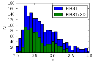
Figure 4 displays the redshift distribution for radio-selected objects (“FIRST”, blue histogram) and those that passed both the radio and XDQSO selection (“FIRST”+XD, green histogram). This graph can be compared directly to Figure 10 in R06, which compares the redshift distribution of radio-selected quasars to those that were both radio- and color-selected using the full DR3Q (Schneider et al., 2005) sample. The redshift distribution of the radio-only selected objects is smoother and has a smaller decrement of objects at $z=2.7-2.8$ than the radio$+$color selection. This was also seen in the R06 DR3Q investigation.

However, we are wary of over-interpreting this for several reasons. First, only $\sim 2$% (3 348) of the DR9Q (Pâris et al., 2012), and $\sim 2$% (747) of the XDQSO quasars are targeted via their radio properties, of which half are selected only via their radio properties. Second, BOSS is deeper than SDSS, whereas the FIRST detection limits are the same for the two optical surveys, so BOSS radio sources are more radio loud. If radio loudness correlates with redshift and/or luminosity (e.g., Jiang et al., 2007; Singal et al., 2011, 2012), an attempt to correct the $N(z)$ distribution using radio-loud quasars would be incorrect (see also the discussion in § 3.4 of R06). Finally, radio-loud quasars are not drawn from the same color distribution as radio-quiet quasars, with the radio-loud population tending to have redder colors (White et al., 2003; McGreer et al., 2009; Kimball et al., 2011). Thus objects in a radio-selected quasar sample do not share the same selection function as a purely color-selected sample.

3.4. Simulated Quasar Spectra and Completeness

In Section 3.2 we presented the sample established by the XDQSO targeting algorithm, and compared it to a dataset constructed from the Stripe 82 sample of quasars selected independently of that algorithm. We can use the results of § 3.2 to quantify the completeness of XDQSO only in the limit that the Stripe 82 sample is itself complete. Here we adopt another approach: we construct a model for the observed spectroscopic and photometric properties of quasars, generate a large sample of simulated quasars, and then test the targeting algorithm against this model using the simulated quasars (e.g., Fan, 1999; Richards et al., 2006b).

The broadband optical fluxes used by XDQSO are dominated by a featureless power-law continuum. However, quasar selection is highly sensitive to the colors of quasars, which evolve strongly with redshift as the broad, high-equivalent-width emission lines move through the optical bandpasses (Richards et al., 2001a). Hence, a complete prescription for quasar properties must capture both the smooth continuum and the emission lines.

Past models have generally adopted a continuum power law index of $\alpha_{\nu}=-0.5$, where $\alpha_{\nu}$ is the frequency power law index (i.e. $F(\nu)\propto\nu^{\alpha_{\nu}}$), typically measured from quasar spectra (e.g., Richstone & Schmidt, 1980; Francis et al., 1991; Vanden Berk et al., 2001). Often a break is added to the near UV where a softer spectrum is observed ($\alpha_{\rm UV}\sim-1.7$, Telfer et al., 2002; Shang et al., 2005, 2011). Emission line templates, including Fe ii complexes, are then generated from composite mean quasar spectra constructed from large samples (e.g., Francis et al., 1991; Vanden Berk et al., 2001). To these emission components, absorption from the Ly$\alpha$ forest is added, given a model for its redshift dependence. With these basic assumptions, models can be generated that broadly reproduce the mean colors of quasars as a function of redshift (Richards et al., 2001a).

For this work we have taken advantage of the many improvements in our understanding of quasar spectral properties in recent years, namely, improved measurements of absorption due to the Ly$\alpha$ forest (e.g., Worseck & Prochaska, 2011), templates for iron emission (a significant contributor to quasar colors; Vestergaard & Wilkes, 2001) and finally, large samples of quasars to calibrate the models. We have simulated the full survey, by passing the model quasars through the target selection algorithm and comparing the resulting color distribution to observations. Under the common assumption that quasar spectral features do not evolve with redshift, the selection function provides a redshift-dependent window into the underlying color distribution. By comparing the colors of quasars that the model predicts are selected by the survey, to those actually observed, we can determine a best-fit model that not only recovers the selection function, but also provides insight into the intrinsic properties of quasars.

Figure 6.— The selection function for the BOSS XDQSO sample via simulated quasar spectra and photometry. Contour levels are drawn at 1, 5, 10, 20, 40, 50, 60, 80, and 90 percent completeness, as determined by the fraction of simulated quasars selected by XDQSO as a function of redshift and $i$-band magnitude. The 50% and 90% levels are drawn with dashed lines.

Figure 7.— BOSS (XDQSO) quasar selection function, in discrete redshift bins covering the range $2.2<z<3.4$. The blue points with error bars show the empirical selection function derived from Stripe 82; specifically, they denote the fraction of Stripe 82 quasars selected by XDQSO within bins of magnitude and redshift (the $x$-error bar represents the $i$-magnitude bin width). The green line shows our “fiducial” model selection function using simulated quasars as described in § 3.4 , and the same binning as the empirical points. The agreement at $z\lesssim 3$ shows that the two are consistent, as expected if both the model is a good representation of true quasars and the variability selection is highly complete. The model predicts lower efficiency at $z>3$, suggesting that the completeness of the variability selection is lower at higher redshifts i.e., XDQSO recovers a higher fraction of the variability quasars than the model quasars, and variability is potentially missing a population of quasars. Note also that the efficiency predicted by the model is generally lower in the faintest magnitude bin ($i\sim 22$), again suggesting that variability was less complete at the faint end. Note that the model has a luminosity function prior (Hopkins et al., 2007) applied. For comparison, we also plot the “VdB lines” and “exp dust” model selection functions (red and cyan lines, respectively), both of which generally show poorer agreement with the empirical points from Stripe 82 than the fiducial model.

This process will be detailed in a forthcoming work (McGreer et al., in prep). Here we briefly outline the steps taken to generate a model for the population of quasars observed (and not observed) by BOSS.

1. We construct a grid of model quasars in ($M$,$z$) space, using the luminosity function from Hopkins et al. (2007). For each quasar we randomly sample the following components:

   1. A broken power-law continuum with a break at 1100Å; at near-UV wavelengths the power law index is drawn from a Gaussian distribution with mean $\alpha_{\nu}=-1.7$ and scatter $\sigma(\alpha_{\nu})=0.3$; for $\lambda>1100$ Å the distribution has a mean $\alpha_{\nu}=-0.5$ and scatter $\sigma(\alpha_{\nu})=0.25$.

   2. Emission lines generated from composite spectra of BOSS quasars binned in luminosity, reproducing trends between emission line properties and continuum luminosity (e.g., the Baldwin Effect: Baldwin, 1977; Wu et al., 2009). The resulting emission line template provides the mean and scatter in line strength for prominent quasar emission lines as a function of luminosity; values for individual objects are drawn from this distribution.

   3. Fe emission from the template of Vestergaard & Wilkes (2001). The template is divided into discrete wavelength segments (see Vestergaard & Wilkes, 2001) that are scaled independently; the scale values are determined during the fitting of the composite spectra used for the emission line template.

   4. Ly$\alpha$ forest blanketing according to the prescription of Worseck & Prochaska (2011). A population of absorbers is generated in a Monte Carlo fashion using the parameters given in Worseck & Prochaska (2011). The lines are modeled as Voigt profiles using the approximation of Tepper-García (2006), and then applied to the forest regions of the simulated spectra. All Lyman series transitions up to $n=32$ are included. A total of 5000 independent sightlines were generated and then randomly drawn for each of the simulated quasars.

2. We generate spectra from this grid and calculate SDSS broadband fluxes from the spectra.

3. The fluxes are transferred to observed values via empirical relations for the photometric uncertainties derived from single-epoch observations of stars on Stripe 82, using the coadded fluxes (Annis et al., 2011) as the reference system.

4. The XDQSO algorithm is used to calculate mid-$z$ quasar probabilities for each model quasar in the same manner as for BOSS selection, and a sample of model quasars is defined.

This describes our fiducial model. We further test two modifications to the fiducial model. For comparison to previous work, we implement a second model where the emission line template is derived from a single composite spectrum and thus does not have any dependence on luminosity. This template comes from the SDSS composite spectrum presented in Vanden Berk et al. (2001) and is referred to as “VdB lines”. This model is closest to that of Richards et al. (2006b). Finally, we test a third model that includes dust extinction from the host galaxy. In this model, individual spectra are extincted using a SMC dust model (Prevot et al., 1984), with values of $E(B-V)$ distributed exponentially around a peak of $0.03$ (e.g., Hopkins et al., 2004). This model is referred to as “exp dust”. We compare the three models in more detail in Appendix A.

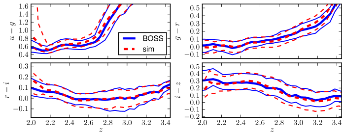
We test the accuracy of the fiducial model by checking the simulated quasar colors against observed quasar colors. This prior is used to distribute the simulated quasars in flux and redshift space in a manner similar to the intrinsic distribution. The simulated quasar photometry is passed through the XDQSO selection algorithm to mimic the observations, so that the final color relations for simulated quasars are derived only for objects that would have been targeted by the survey. We then construct the color-redshift relation (e.g., Richards et al., 2001a) of both simulated and observed quasars by dividing the samples into narrow redshift bins ($\Delta z=0.05$) and calculating both the median and scatter of the $u-g$, $g-r$, $r-i$, and $i-z$ colors within each redshift bin. The results for the fiducial model are shown in Figure 5, demonstrating that the model does an excellent job of reproducing the observed quasar color distribution.

Dust extinction is thought to produce the red tail of the color distribution often seen in quasar surveys. For example, Richards et al. (2003) and Hopkins et al. (2004) find that $\sim 20$% of SDSS quasars have colors consistent with reddening from dust with an SMC-like extinction curve with $E(B-V)\gtrsim 0.1$. We find that the exp dust model does not significantly improve the fit to the color distribution of BOSS quasars compared to our fiducial model, and thus our primary analysis does not include the effect of dust extinction. Section 5 will explore how the differing assumptions of the three models affect the calculation of the QLF.

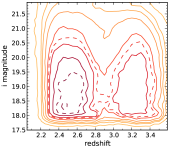
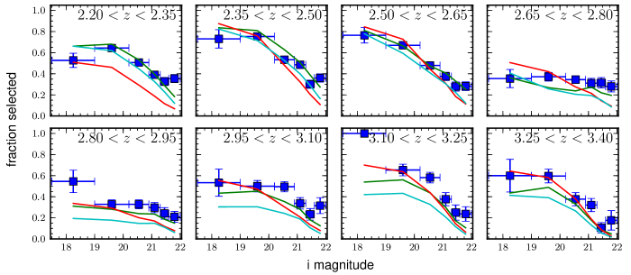
Table 5 and Fig. 6 give the selection function, i.e. the fraction of selected quasars, in each bin of $M$ and $z$, generated from the fiducial model outlined above.

$i$_start	$i$_end	$z$_start	$z$_end	Selec. Func.
17.500	17.600	2.000	2.050	0.0000
17.500	17.600	2.050	2.100	0.0000
$\vdots$	$\vdots$	$\vdots$	$\vdots$	$\vdots$
17.800	17.900	2.100	2.150	0.0000
17.800	17.900	2.150	2.200	0.0291
17.800	17.900	2.200	2.250	0.1710
17.800	17.900	2.250	2.300	0.4076
17.800	17.900	2.300	2.350	0.3365
17.800	17.900	2.350	2.400	0.5029

Table 5The Quasar Selection Function for the fiducial model described in the text; see also Fig. 6. The final column gives the fraction of simulated quasars selected by XDQSO. Table 5 is published in its entirety in the electronic edition of The Astrophysical Journal; this excerpt here is shown here for guidance regarding its format and content.

We compare the model selection function to an empirical relation from Stripe 82 in Figure 7. The green lines show the fraction of model quasars that are selected by XDQSO-CORE. This is compared to the fraction of Stripe 82 quasars — predominantly selected by variability criteria — that are recovered by XDQSO selection. This empirical relation is shown as blue squares with error bars (Poisson uncertainties). The agreement at $z\lesssim 3$ shows that the two are consistent, as expected if both the model is a good representation of actual quasars, and the variability selection is highly complete.

However, there is some disagreement between the two completeness estimates. For example, smaller fractions of model quasars are selected by XDQSO at $z>3$ than are selected by XDQSO from the Stripe 82 sample in the same redshift and magnitude bins. This may indicate a deficiency of the models; however, we are encouraged by the excellent agreement between the colors predicted by the model and those observed (Figure 5). Alternatively, our assumption that the variability-selected sample is both complete and unbiased may be invalid. Indeed, color criteria were applied to objects when constructing the variability sample (Palanque-Delabrouille et al., 2011); these criteria may exclude some populations of quasars, in particular, they may introduce bias against high redshift quasars. In that case, the disagreement in Figure 7 suggests that XDQSO recovers a higher fraction of the variability-selected quasars, but both XDQSO and variability are missing a population of objects. This effect may also explain why the model predicts lower completeness at the faintest magnitudes: i.e., both XDQSO and variability have low completeness at $i\sim 21.8$, but XDQSO recovers a higher fraction of the quasars that are also selected by variability.

In what follows, we implement our fiducial selection function model to calculate the QLF from the DR9 uniform quasar sample. Since the color selection incompleteness dominates over the other sources of incompleteness, we do not make any further corrections during the QLF calculation.

Figure 8.— Cumulative $i$-band number counts. Here, the $2.2<z<3.5$ BOSS samples are in red, with the uncorrected BOSS uniform sample shown by the open circles, while the Stripe 82 data are given by the crosses. Also shown are the number counts from the deeper, $g\approx 23$ $1.0<z<2.2$ quasars selected from the “boss21+MMT” survey (Palanque-Delabrouille et al., 2012). For clarity, we only plot errorbars at the bright end ($i<19$), since the errors are smaller than the points at the faint end. We also show the double power law fits to the data as described in the text.

Figure 9.— Comparison of the $k$-correction from our fiducial model (blue line) with the R06 $k$-correction (green line). Both are defined as the correction required to transfer the observed $i$-band flux to the $i$-band luminosity at $z=2$, i.e., $M_{i}(z=2)$. The offset of $\sim$0.1 mag at $z<2.7$ is due to a different treatment of Fe emission, and grows somewhat larger at higher redshifts as the C iii] line enters the $i$-band. The blue line shows our quasar model for $M_{i}(z=2)=-26$, and the shaded regions show the variation of the $k$-correction with luminosity over the range $-27<M_{i}(z=2)<-24.3$, covering most of the luminosity range of BOSS quasars. Finally, the dashed line shows a pure continuum $k$-correction for $\alpha_{\nu}=-0.5$.

4. Number Counts and $k$-corrections

4.1. Number Counts

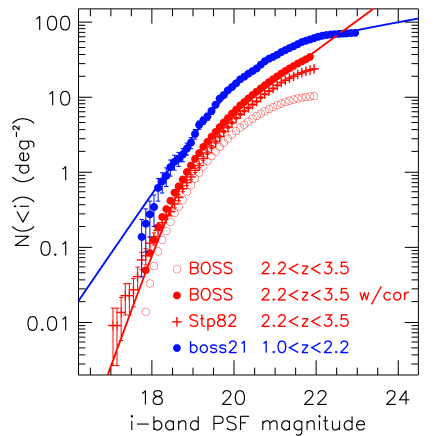
In Fig. 8 we present the cumulative $i$-band number counts of the datasets described in Sec. 2: the XDQSO uniform sample of 23 301 quasars across 2236 deg² with $2.2<z<3.5$ (red circles) and the 5 470 quasars across 220 deg² of Stripe 82 also with $2.2<z<3.5$ (red crosses). Also shown are the number counts from $1.0<z<2.2$ quasars selected from deeper, $g\approx 23$ spectroscopy, using data from the “boss21+MMT” survey (blue, filled circles; Palanque-Delabrouille et al., 2012).

For the uniform BOSS sample, the open red circles are for the raw, uncorrected number counts, whereas the filled circles use the correction derived in the previous section, integrated over our redshift range. These number counts can be compared to the $2.2<z<3.5$ quasars selected via their variability signature on Stripe 82. The two are in reasonable agreement to $i\approx 21.0$, with the corrected number counts being consistently higher. Fainter than this, the variability number counts drop more noticeably below the corrected counts, suggesting that this dataset is incomplete at the faint end (or that the incompleteness of the DR9 sample is overestimated). Across the redshift range $2.2<z<3.5$ and down to $i=21.5$, the corrected BOSS DR9 uniform cumulative number counts reach 34.4 deg^-2, whereas the Stripe 82 cumulative counts are 26.2 deg^-2.

Motivated by the double power-law form of the QLF (Eqn. 2), and prior measurements (e.g. Myers et al., 2003), we also express the cumulative number counts as a double power-law,

$$\int dN=\frac{N_{0}}{10^{-\alpha_{d}(m-m_{0})}+10^{-\beta_{d}(m-m_{0})}}$$ (3)

and find best-fits to the (corrected) BOSS uniform and boss21+MMT counts. For the BOSS sample we find slopes of $\alpha_{d}=1.50$ and $\beta_{d}=0.40$, while the “break magnitude” $m_{0}=$19.0 and the normalization, $N_{0}=2.63$ deg^-2. In comparison, the boss21+MMT data has a less-steep bright end slope of $\alpha_{d}=0.80$ and an almost flat faint end slope $\beta_{d}=0.10$. The break magnitude is fainter at $m_{0}=20.4$ and the normalization is significantly higher, $N_{0}=43.6$ deg^-2. These power-law descriptions and surface densities will allow extrapolation for future Ly$\alpha$-forest cosmology experiments (e.g., McQuinn & White, 2011). For unobscured $1.0<z<2.2$ quasars, there are 48 (78) objects deg^-2 down to $i\lesssim 21.5$ (23.0), broadly consistent with the value of 99$\pm$4 quasars deg^-2 with $g_{\rm dered}<22.5$ from Palanque-Delabrouille et al. (2012, their Table 5) and a surface density similar to that selected by a shallow mid-infrared selection (Stern et al., 2012; Yan et al., 2012).

$z_{\rm em}$	$k$-correction
0.105…………..	0.323
0.115…………..	0.250
0.125…………..	0.317
0.135…………..	0.332
0.145…………..	0.335
0.155…………..	0.334
0.165…………..	0.285
0.175…………..	0.291
0.185…………..	0.334
0.195…………..	0.249

Table 6 The $i$-band $k$-corrections. The $k$-correction is obtained using the fiducial quasar model described in Section 3.4, and includes an updated treatment of the emission line template compared to Richards et al. (2006b). We define our $k$-correction to be our model $k$-correction at $M_{i}(z=2)=-26.0$ (see main text for details). The full table is published in the electronic edition of The Astrophysical Journal; the first ten lines are shown here for guidance regarding its format and content.

4.2. $k$-corrections

Following R06, we define the $k$-correction to determine the $i$-band luminosity at $z=2$; $M_{i}(z=2)$. This is $\sim$2700 Å in the rest-frame, and is close to the median redshift of the BOSS quasars sample. R06 calculate the quasar $k$-correction as the sum of a component due to the underlying continuum, $k_{\rm cont}$, and a component due to the emission lines, $k_{\rm em}$. The sign convention of the $k$-correction, $k(z)$, is $m_{\rm intrinsic}=m_{\rm observed}-k(z)$ (Oke & Sandage, 1968; Hogg et al., 2002).

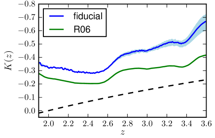
We obtain a $k$-correction from the fiducial quasar model defined in Section 3.4. This model is very similar to the one adopted by R06. The continuum model is identical: a power-law slope of $\alpha_{\nu}=-0.5$ at $\lambda>1100$Å, and we set $k_{\rm cont}(z=2.0)=0.0$ by definition. On the other hand, our emission line template is not the same as the one used by R06. They defined their emission line template using a single composite spectrum derived from SDSS quasars (similar to that of Vanden Berk et al., 2001) with a power-law continuum removed. Our emission line template is similarly obtained from composite spectra; however, we use a suite of composite spectra binned in luminosity, and fit the continuum jointly with the Fe template of Vestergaard & Wilkes (2001).

One advantage of defining the $k$-correction to be in the $i$-band at $z=2$ is that the $i$-band is relatively free of strong emission lines at this redshift. At $z\lesssim 2.5$, the $i$-band samples rest-frame $\sim 2200$Å, where the only strong emission line features are from Fe II and Fe III. We find that our model for Fe emission introduces a shift of about $\sim$0.1 mag at $2<z<2.7$ relative to the R06 model; i.e., $k_{\rm fid}-k_{\rm R06}\approx-0.1$. At higher redshifts, the C iii] line enters the $i$-band and the offset between our $k$-correction and that of R06 grows somewhat larger, reaching $\approx-0.2$ mag at $z=3.5$. We compare our $k$-correction to that of R06 in Figure 9.

Figure 10.— The Absolute Magnitude-Redshift distribution for SDSS DR7 quasars (black points), BOSS DR9 (red points) and the fainter, boss21+MMT variability-selected dataset from Stripe 82 (blue squares). The normalized redshift distributions of the three datasets are shown in the bottom panel, while the normalized absolute i-band magnitudes are given in the side panel. The bright and faint magnitude limits of the BOSS DR9 sample are given by the solid turquoise lines; the wiggles are due to the redshift dependence of the $k$-correction.

Though our quasar model introduces a luminosity dependence to the $k$-correction due to the anticorrelation between emission line equivalent width and luminosity (the Baldwin Effect), we chose not to apply this further correction in this work. For the same reasons given above, at $z<2.7$ there is almost no variation in our $k$-correction with luminosity. At $z=3.5$, this effect only reaches $\sim 5\%$ over the range of luminosities probed by BOSS (see Figure 9). This variation is much smaller than the intrinsic scatter in $k$-corrections at a given redshift; i.e., even if we attempted to correct for the Baldwin Effect in the mean, the scatter in this correlation is far greater than the correction. We define our $k$-correction to be our model $k$-correction at $M_{i}(z=2)=-26.0$, near the median luminosity of the BOSS sample. Table 6 presents our new $k$-correction.

$\bar{z}$	$\langle M_{i}(z=2)\rangle$	$M_{i}$ bin	$N_{\rm Q}$	$\log(\Phi)$	$\sigma_{\Phi}/10^{-9}$
(1)	(2)	(3)	(4)	(5)	(6)
2.488	-28.297	-28.350	26	-7.892	1.994
2.386	-28.024	-28.050	105	-7.338	3.772
2.409	-27.737	-27.750	184	-7.125	4.821
2.399	-27.437	-27.450	306	-6.917	6.126
2.408	-27.143	-27.150	510	-6.699	7.874
2.397	-26.844	-26.850	825	-6.486	10.063
2.392	-26.544	-26.550	1037	-6.360	11.631
2.391	-26.246	-26.250	1382	-6.210	13.824
2.381	-25.948	-25.950	1604	-6.104	15.629
2.385	-25.653	-25.650	1778	-5.983	17.958
2.378	-25.351	-25.350	1878	-5.855	20.808
2.375	-25.051	-25.050	1768	-5.824	21.562
2.373	-24.758	-24.750	1484	-5.807	21.991
2.364	-24.457	-24.450	1059	-5.750	23.483
2.332	-24.187	-24.150	456	-6.143	14.936
2.296	-23.907	-23.850	58	—	—
2.216	-23.678	-23.550	2	—	—
2.830	-28.566	-28.650	5	-8.127	1.527
2.761	-28.328	-28.350	46	-7.469	3.259
2.787	-28.032	-28.050	67	-7.304	3.939
2.796	-27.739	-27.750	120	-7.013	5.509
2.802	-27.440	-27.450	217	-6.750	7.452
2.782	-27.145	-27.150	291	-6.630	8.557
2.780	-26.845	-26.850	373	-6.483	10.131
2.777	-26.547	-26.550	484	-6.301	12.501
2.775	-26.239	-26.250	512	-6.210	13.876
2.775	-25.944	-25.950	536	-6.206	13.949
2.776	-25.651	-25.650	646	-6.109	15.595
2.773	-25.362	-25.350	669	-6.046	16.762
2.776	-25.056	-25.050	634	-5.975	18.188
2.764	-24.758	-24.750	382	-6.079	16.129
2.715	-24.487	-24.450	184	-6.552	9.362
2.681	-24.217	-24.150	25	—	—
3.259	-28.864	-28.950	3	-8.588	0.815
3.283	-28.627	-28.650	25	-7.754	2.128
3.207	-28.327	-28.350	44	-7.543	2.711
3.219	-28.063	-28.050	72	-7.406	3.174
3.208	-27.746	-27.750	136	-7.131	4.356
3.206	-27.441	-27.450	218	-6.899	5.691
3.208	-27.141	-27.150	265	-6.803	6.358
3.190	-26.848	-26.850	371	-6.666	7.448
3.185	-26.539	-26.550	460	-6.551	8.494
3.181	-26.250	-26.250	515	-6.492	9.090
3.173	-25.954	-25.950	486	-6.426	9.817
3.170	-25.658	-25.650	402	-6.317	11.131
3.153	-25.359	-25.350	332	-6.174	13.114
3.138	-25.062	-25.050	218	-6.040	15.306
3.127	-24.800	-24.750	85	-6.329	10.966
3.097	-24.486	-24.450	16	—	—

Table 7The binned BOSS DR9 Quasar Luminosity Function. (1) The mean redshift of the bin; (2) The mean $i$-band absolute magnitude of the bin; (3) the absolute magnitude bin center; (4) The number of quasars in each bin; (5) $\Phi$ in units of Mpc^-3 mag^-1 and (6) The (Poisson) error on $\Phi$, divided by $1\times 10^{-9}$; The bins with no measured $\Phi$ are at the faint end limit where the selection function is rapidly approaching, or is equal to, 0.00, thus making our QLF estimation very uncertain. However, these bins are included so that $\sum N_{\rm Q}=23\,301$.

5. Luminosity Functions

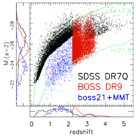
In Fig. 10, we show the coverage in the absolute magnitude-redshift ($M_{i}-z$) plane for the three datasets of main interest here: the SDSS (black points; Richards et al., 2006b; Schneider et al., 2010); the XDQSO-selected $2.2\leq z\leq 3.5$ BOSS DR9 sample (red points) and the fainter variability-selected dataset from the boss21+MMT sample (blue squares; Palanque-Delabrouille et al., 2012). We also analyze the Stripe 82 variability-selected dataset of Palanque-Delabrouille et al. (2011), which has a similar redshift distribution as the DR9 sample. The bright and faint magnitude limits of the BOSS DR9 sample, $i=17.8$ and $i=21.8$, respectively, are given are given by the solid turquoise lines. Our binning is identical to R06; the edges of the redshift bins in which we will calculated the QLF are: 0.30, 0.68, 1.06, 1.44, 1.82, 2.20, 2.6, 3.0, 3.5, 4.0, 4.5, and 5.0, and the $M_{i}$ bins start at -22.5 and are in increments of 0.30 mag.

Figure 11.— The $i$-band Quasar Luminosity Function. The red points are from our analysis of BOSS quasars from DR9, while the black squares are from the DR3 analysis of Richards et al. (2006b). The boss21+MMT sample from Palanque-Delabrouille et al. (2012) is also shown for $0.68<z<2.20$ (blue filled squares). Over the redshift range $2.20\leq z\leq 3.50$, we use the 23 301 DR9 quasars uniformly selected by XDQSO, and that are in sectors of spectro-completeness of 85% or higher. The solid line in each panel is the BOSS DR9 QLF at $2.2<z<2.6$, to show how the luminosity function evolves. The open circles show the $2.2<z<3.5$ QLF without correcting for the (fiducial) selection function. There are no uniform DR9 measurements above $z=3.5$, since the XDQSO selection deliberately cuts off at this redshift. The Poisson error bars for the BOSS measurements in the three panels spanning $2.2<z<3.5$ are the same size, or smaller, than the points shown.

5.1. The Optical Luminosity Function to $i=21.8$

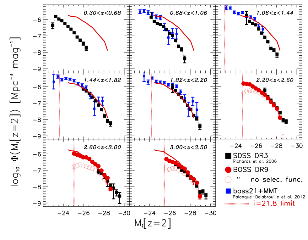
In Fig. 11 we show the $i$-band luminosity function from our BOSS DR9 uniform sample over $2.2<z<3.5$, as well as the fainter boss21+MMT sample of quasars covering $0.68<z<2.2$ from Palanque-Delabrouille et al. (2012). We use the binned QLF estimator of Page & Carrera (2000),

$$\phi\approx\phi_{\rm est}=\frac{N_{q}}{\int^{L_{\rm max}}_{L_{\rm min}}\int^{z_{\rm max}(L)}_{z_{\rm min}}(dV/dz)\ dz\ dL}.$$ (4)

This involves calculating the number of quasars, $N_{q}$ observed in a given ($M_{i}-z$) bin, correcting for our selection function, and dividing $N_{q}$ by the effective volume element $dV$ of that bin. The effective volume is calculated by using our fixed, flat $(\Omega_{\Lambda},\Omega_{\rm m},h)=(0.70,0.30,0.70)$ cosmology, and the area of our uniform DR9 sample (2236 deg²). We check, and find that our redshift bins are sufficiently narrow to avoid complications due to evolution. The plotted error is estimated by

$$\delta\phi_{\rm est}=\frac{\delta N}{\int^{L_{\rm max}}_{L_{\rm min}}\int^{z_{\rm max}(L)}_{z_{\rm min}}(dV/dz)\ dz\ dL}$$ (5)

and $\delta N$ is given by Poisson statistics including the up-weighting by the inverse of the completeness. We discuss the validity of this error estimate below. The binned QLF is also given in Table 7, which gives the mean redshift of the quasars in each bin, the mean $i$-band magnitude of the quasars in the bin, the magnitude at the bin center, the raw number of quasars in the bin, the log of the space density, $\Phi$, in Mpc^-3 mag^-1, and the error $\times 10^{9}$. The results from R06 using the SDSS DR3 are given as the black squares in Fig. 11. Shen & Kelly (2012) measured the QLF from the final DR7 SDSS quasar sample, and found excellent agreement with the DR3 results.

Figure 12.— The sensitivity of the BOSS DR9 Quasar Luminosity Function to the selection function models used. The QLF is divided by the fiducial model. The red points show this fiducial model (at 0 by definition), with the extent of the points representing the statistical uncertainty range. The QLFs derived from the other two models are divided by the fiducial model QLF to highlight the effect of the choice of selection function on the derived QLF. The VdB lines model is shown as green points, and the exp dust model as blue points. In general there is good agreement between the three models, but in some redshift bins the disagreement can be 20% or greater. The fiducial model provides the best fit to the observed color-redshift relation; however, the differences seen here quantify the systematic uncertainty inherent in not knowing the selection function exactly.

Where the surveys overlap, we generally see very good agreement with the BOSS and SDSS data points, especially at $z\leq 3$. Although there is overlap in $L-z$ coverage between the SDSS DR3 and BOSS measurements, since DR3 and DR9 cover different ares of the sky, there are only 304 quasars ($\lesssim 2$%) are common to both surveys, mostly in the $3<z<3.5$ redshift range.

The limiting magnitude for BOSS DR9 quasar targets is $g<22.00$ or $r<21.85$, and with $(r-i)\approx 0.05$ for quasars at $z\approx 2.5$, we show an $i$-band limiting of $i=21.8$ as a guide in Fig. 11. There is strong evidence for a turn-over in the QLF, well before this limit, seen in all the redshift panels i.e. up to $z=3.5$. We shall see in Sec. 5.2, that our results across $3.0<z<3.5$ are also consistent with a turn over seen in other experiments. This turn-over has been seen in the X-rays (Miyaji et al., 2001; Ueda et al., 2003; Hasinger et al., 2005; Aird et al., 2010; Fiore et al., 2012) and also in the optical (Boyle et al., 1988; Croom et al., 2004; Croom et al., 2009a), with the BOSS DR9 now extending this evidence to redshifts $z=3.5$.

Figure 13.— The i-band Quasar Luminosity Function. Black squares are from Richards et al. (2006b), the filled red circles are our measurements from the full DR9 sample, while the teal points are from our analysis of the 5,476 BOSS quasars with $2.2<z<3.5$ located and observed on Stripe 82. The top-left panel is the 2.2$<z<$2.6 measurement from Fig. 11 shown as a guide.

Our calculation of the errorbars given in Fig. 11 assumes the errors in each bin are independent and are dominated by Poisson statistics of the observed objects. For the DR9 sample overall this is reasonable, given the very large volume surveyed (which reduces fluctuations due to large-scale structure) and the low mean occupancy of quasars in halos (which reduces the impact of halo count fluctuations on the correlations). When comparing to surveys of smaller volume, sample variance may dominate over the Poisson errors. In some redshift ranges, however, BOSS is quite incomplete, and require a significant selection function correction (compare the open red circles to the filled red circles in the $2.6<z<3.0$ bin of Fig. 11 for example). In these bins the error is dominated not by Poisson statistics but by the uncertainty in our estimate of the selection function (see Fig. 7). This uncertainty can reach 50%, fractionally, for faint quasars in the most incomplete redshift range, leading to a similar fractional uncertainty in the QLF. However for most of the range plotted the uncertainty is significantly smaller.

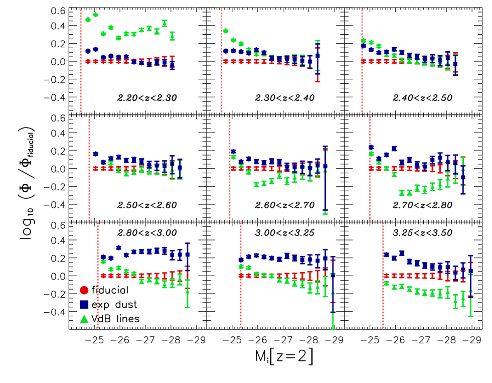
In Fig. 12 the effect of the selection function correction is investigated further. Here we plot the logarithm of the ratio of the QLF number densities for the two other selection function models, “VdB lines” and “exp dust”, introduced in Sec. 3.4, compared to our fiducial model (that is used to calculate the QLF presented in Fig. 11). We concentrate on the redshift range $2.20<z<3.50$. The errorbars for each model represent the Poisson uncertainties, and the differences between selection function models dominate over these statistical uncertainties, especially at the faint end. The corrections derived from the exp dust model generally augment the estimated luminosity function, particularly at low luminosities and higher redshifts. This is likely due to the fact that BOSS quasar selection is flux-limited in the $g$ and $r$ bands, so that fainter and higher redshift objects subjected to dust reddening will be extincted out of survey selection. The corrections derived from the VdB lines model show an even stronger trend with luminosity. The dependence of observed quasar colors on intrinsic luminosity resulting from the Baldwin Effect leads to a luminosity-dependent selection function. A QLF estimate that does not account for this effect will incur an artificial tilt as a function of luminosity, as highlighted by the figure. This tilt will further affect QLF parameters such as the power law slopes.

Figure 14.— The BOSS DR9 Quasar Luminosity Function compared to other surveys. Left: Measurement in the $1.8<z<2.2$ range using data from BOSS (this paper; red circles), SDSS (black squares; Richards et al., 2006b), 2SLAQ QSO survey (light blue up-triangles; Croom et al., 2009a), the “boss21+MMT” survey (dark blue circles; Palanque-Delabrouille et al., 2012) and the COMBO-17 survey (orange down-triangles; Wolf et al., 2003). Center: Measurement in the $2.2<z<2.6$ range; Right: Measurement at $z\sim 3.2$, now adding data from the COSMOS survey (purple diamonds; Masters et al., 2012) and SWIRE (dark green squares; Siana et al., 2008). In each panel, we have divided the various QLFs by our best-fit “log-linear” LEDE model, which is described below in Sec. 6.1 and Table 8.

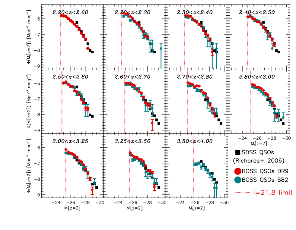
In Fig. 13, we continue to concentrate on the redshift range $2.2\leq z\leq 3.5$, and divide it more finely in redshift than in Fig. 11. The data displayed in Fig. 13 are presented in tabular form in Appendix B, and it will be these data that we will fit models to in Sec. 6.1. We compare the BOSS DR9 measurements to the 5 476 $2.2<z<3.5$ quasars on Stripe 82 that were selected via variability. The BOSS DR9 and Stripe 82 measurements are in very good agreement below $z\sim 2.7$, consistent with the selection function agreement in Fig. 7.

However, there are differences between the two datasets for $z\gtrsim 2.7$, especially at the fainter end. The DR9 measurement implies a higher space density than the Stripe 82 variability measurements. One possible explanation could be that the selection function is underestimated (in the sense that it over corrects $N_{q}$) from Sec. 3.4. However, this would potentially lead to higher DR9 space densities at the faint end at all redshifts. Another possibility is that the variability selection is beginning to break down at the faint end, as the selection is based on light-curves taken from single-epoch imaging, and is susceptible to imaging incompleteness.

5.2. Comparison to Other Results

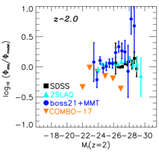
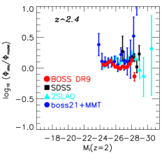
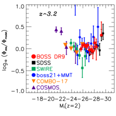
In Fig. 14, we compare our BOSS DR9 QLF to other measurements of the QLF at $z\geq 2$. In each panel, we divide the QLFs by our best-fit “log-linear” Luminosity Evolution and Density Evolution (LEDE) model, described in Section 6.1. We concentrate on the redshifts $z\approx 2.0$ and $z\approx 2.4$, and the results of Croom et al. (2009a) from the 2SLAQ QSO survey. We also compare our measurements at $z\approx 3.2$ with recent results from Masters et al. (2012) using observations from COSMOS (Scoville et al., 2007b). We additionally compare the results from our sister study, Palanque-Delabrouille et al. (2012), at all three epochs.

The 2SLAQ results are presented in Croom et al. (2009a) as a function of $M_{\rm g}(z=2)$, and the COSMOS results in Masters et al. (2012) in $M_{\rm 1450}$, so in order to make a direct comparison, we convert these to $M_{\rm i}(z=2)$, with the transformation:

$$M_{\rm i}(z=2) = M_{\rm g}(z=2)-0.25$$ (6)

$$= M_{\rm 1450}-0.29.$$ (7)

One underlying assumption in these conversions is that the 2SLAQ, and indeed the BOSS, quasars have a distribution in spectral power-law slopes ($\alpha_{\nu}$, where $F(\nu)\propto\nu^{\alpha_{\nu}}$) in the UV/Blue/Optical that is comparable to that of the SDSS quasar sample. Although the BOSS target selection avoids sources that would satisfy a UV Excess selection (see Ross et al., 2012; Pâris et al., 2012), there is not strong a priori reason to suspect that these populations would deviate from a range of intrinsic slopes $-1<\alpha_{\nu}<0$, centered around $\alpha_{\nu}\sim-0.40$.

Our comparison to the 2SLAQ result is shown in the left and center panels of Fig. 14, for the redshift range $1.8\lesssim z\lesssim 2.2$ and $2.2\lesssim z\lesssim 2.6$, respectively. We note that the 2SLAQ result is based on a combination of the 2SLAQ QSO survey (which dominates the signal at the faint end of the QLF) and the SDSS results from DR3 (which is responsible for the bright end measurement). Thus, the 2SLAQ points, represented as light blue upwards-pointing triangles in Fig. 14, are not independent from the SDSS (black) squares.

Concentrating on the $z\approx 2.0$ panel, at the bright, $M_{i}(z=2)<-26$, end the boss21+MMT points, given by the blue filled points, seem $\sim$0.2-0.4 dex higher than e.g. the 2SLAQ and SDSS data, though are generally consistent within the quoted (statistical) error. Palanque-Delabrouille et al. (2012) explore the variability selection in more detail than presented here, and resolution of this issue will be aided by new, forthcoming, variability-selected data, since sample variance uncertainties over the 14 deg² boss21+MMT field could well be an issue. At the faint end, boss21+MMT, 2SLAQ and SDSS are all consistent. All the displayed measurements are consistent with the COMBO-17 points (orange down-triangles), due to the large error associated with those points (not shown).

At $z\sim 2.4$ the BOSS DR9, SDSS, 2SLAQ and “boss21+MMT” are in excellent agreement, at both the bright and faint ends.

We compare to the COSMOS result at $z\sim 3.2$ (Masters et al., 2012), in the right panel of Fig. 14. The BOSS QLF measurement is in good agreement with the COSMOS results, given by the purple upward-pointing triangles. We also plot results from Siana et al. (2008, green squares), who use an optical/infra-red selection over 11.7 deg² from the Spitzer Wide-area Infrared Extragalactic (SWIRE; Lonsdale et al., 2003) Legacy Survey. The measurements from the $3<z<3.5$ bin from Palanque-Delabrouille et al. (2012) is also given (blue circles). The BOSS DR9, SDSS, and boss21+MMT data are all in good agreement, and consisent given the errors. The faintest BOSS points are consistent with the brightest SWIRE, COMBO-17 and COSMOS points, again given the associated errors. There seems to be an inflection around $M_{i}(z=2)\approx-25.5$, suggesting that our best-fit model is under-predicting the QLF at the both the bright and faint end, i.e. the bright end slope of the model is too steep, while the faint end slope is too shallow. We discuss this further in Sec. 6.1.

The R06 points lie below the other determinations, suggesting that they slightly underestimated the number density of $3.0<z<3.5$ quasars. Worseck & Prochaska (2011) used UV data from the GALEX satellite (Martin et al., 2005; Morrissey et al., 2007), to show that the SDSS quasar target selection systematically misses quasars with blue $u-g\lesssim 2$ colors at $3\lesssim z\lesssim 3.5$ and preferentially selects quasars at these redshifts with intervening H i  Lyman limit systems, causing the QLF to be underestimated. Indeed, we specifically use the Worseck & Prochaska (2011) Monte Carlo model to describe the H i  Lyman series/forest and continuum absorption when creating our BOSS selection function, so we have corrected for this effect.

6. QLF Fits, Models and Discussion

In this section, we fit parametric models to our binned QLF and examine the evolution of the fitted parameters with redshift. We then compare our data to predictions based on more physical models of quasar evolution. Finally, we place our results in a broader context regarding the AGN population and its link to galaxy evolution.

6.1. QLF model fits

The QLF is traditionally fit by a double power-law of the form in Eq. 1. This functional form has four basic parameters, and various phenomenological models have been proposed to describe how those parameters evolve with redshift. In Pure Luminosity Evolution (PLE), only the break magnitude/luminosity evolves, leaving the overall number density constant. The opposite occurs in Pure Density Evolution: the shape of the QLF remains constant while the number density evolves. Various hybrid models allow both to vary but hold the bright- and faint-end slopes fixed. In Luminosity Evolution and Density Evolution (LEDE), $M_{\rm i}^{*}(z)$ and $\Phi^{*}(z)$ evolve independently, while in Luminosity Dependent Density Evolution (LDDE), the evolution of $\Phi^{*}(z)$ is related to that of $M_{\rm i}^{*}(z)$. Finally, extensions to these models allow the power law slopes to evolve as well.

We begin with a simple PLE model for our data. In principle, $M_{\rm i}^{*}(z)$ can take any functional form, but we follow Boyle et al. (2000) by fitting it with a second order polynomial:

$$M_{\rm i}^{*}(z)=M_{\rm i}^{*}(z=0)-2.5(k_{1}z+k_{2}z^{2})~{}.$$ (8)

We note that this quadratic form for $M_{\rm i}^{*}(z)$ requires symmetric evolution about the brightest $M_{\rm i}^{*}$ value, and that this is known to break down at redshifts well above the peak (e.g. Richards et al., 2006b). However, we are motivated to continue to use the quadratic PLE description as a historical reference and because over a limited redshift range the general form of our QLF is qualitatively consistent with a PLE model. For example, if the solid red line (representing the BOSS DR9 QLF at $2.2<z<2.6$) in Fig. 11 is compared to the measured QLF at $z\lesssim 3$, one sees the broader trends in the data are encapsulated by a shift in $M_{\rm i}^{*}$ with little change in normalization.

We fit the PLE model with Eqn. 8 to our data over various redshift ranges. We use the combination of SDSS (R06), boss21+MMT and BOSS Stripe 82 dataset to perform the fits. These data span $0.30<z<4.75$ in redshift, $-29.55\leq M_{\rm i}(z=2)\leq-22.96$ in magnitude and $\Phi=2.2\times 10^{-9}-2.2\times 10^{-6}$ Mpc^-3 mag^-1 in number density. We fit to the Stripe 82 data, since we expect that this data is less affected by systematics, and thus more meaningful $\chi^{2}$ values can be obtained from the statistical uncertainties. We have also found that the S82 data is a fair representation of the DR9 data (Fig. 13).

We perform $\chi^{2}$ fits to the binned data with six total free parameters in the PLE model, using the Levenberg-Marquardt optimization method to find the best-fit parameters by minimizing the $\chi^{2}$. The parameter values for our best-fit PLE models are given in Table 8. We first restrict our fits to $z<2.2$, where previous work has generally found that PLE models provide a reasonably good fit. Fitting over $0.30<z<2.20$ results in $\chi^{2}/\nu=155/75$. Most of the disagreement with our data comes at $z<1$; by restricting to the range $1.06<z<2.20$ the fit improves to $\chi^{2}/\nu=83/52$. Thus we find that PLE models do indeed provide a reasonable description of our low redshift data, though clearly there is room for improvement in the $\chi^{2}$. At higher redshift, the PLE model fails. Within the BOSS redshift range of $z=2.20-3.50$ we have $\chi^{2}/\nu=286/113$; the result is even worse over the full redshift range of our data ($z=0.30-3.50$), with $\chi^{2}/\nu=662/195$.

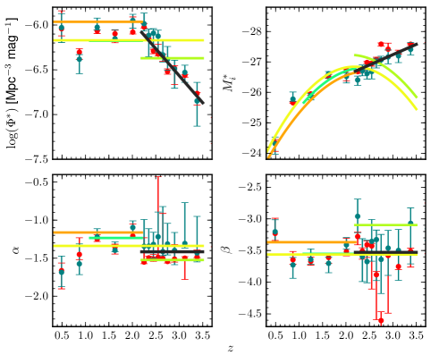
Fig. 15 demonstrates why this is the case, and where the PLE model breaks down. Here we show the behavior with redshift of the parameters $\Phi^{*}$, $M_{\rm i}^{*}$, $\alpha$ and $\beta$. The parameter values and uncertainties are determined by $\chi^{2}$ minimization in each redshift bin independently. In the top right panel, we see that although at $z\lesssim 2.2$, a quadratic description of the evolution of $M_{\rm i}^{*}$ describes the general trend of the data, at $z\gtrsim 2.2$, $M_{\rm i}^{*}(z)$ continues to get brighter and does not exhibit the turn over needed for the parameterization given in equation 8 to work. However, even if a new description of the evolution of $M_{\rm i}^{*}$ could be found, the PLE model, with no allowance for density evolution, is not suitable. This is shown by the top left panel of Fig. 15; we can see that there is essentially no evolution of $\Phi^{*}$ across the range $0.5<z\lesssim 2.2$, but then $\log\Phi^{*}$ declines in a roughly linear fashion with redshift at $z\geq 2.2$, corresponding to a drop in $\Phi^{*}$ by a factor of $\sim$6 between $z=2.2$ and $z=3.5$.

Motivated by the evolution of $\log\Phi^{*}(z)$ and $M_{\rm i}^{*}(z)$ seen in Fig. 15 across the range $z=2.2-3.5$, we implement a form of the LEDE model where the normalization and break luminosity evolve in a log-linear manner; e.g.,

$$\log[\Phi^{*}(z)] = \log[\Phi^{*}(z=2.2)]+c_{1}(z-2.2)$$ (9)

$$M_{\rm i}^{*}(z) = M_{\rm i}^{*}(z=2.2)+c_{2}(z-2.2).$$ (10)

For the BOSS Stripe 82 data across the redshift range $z=2.2-3.5$, this returns a value of $\chi^{2}/\nu=136/113$, indicating a reasonable fit to the data. If we instead fit to the BOSS DR9 data, we find generally good agreement in the fitted parameters, but a dramatically worse $\chi^{2}$ value. While the binned QLF data from DR9 and Stripe 82 are in good agreement, the statistical uncertainties in the DR9 data are far smaller due to the much greater number of quasars. This inflates the $\chi^{2}$ for the same model fit; however, as explained in Sections 3.4 and 5.1, we expect the true uncertainties of the DR9 data to be dominated by systematics, in particular, in the need to correct for color selection effects without knowing the true distribution of quasar colors. The systematic effects associated with correcting for the selection function are obviously a general problem, and are especially problematic as the selection function affects the points in a correlated way. Here we have taken advantage of two quasar samples selected by independent means; we leave this as a cautionary note for surveys relying on an unknown selection function, particularly where the data is dominated by objects found in regions where the selection efficiency is low.

We do not extend our LEDE model below $z=2.2$, where it clearly would not describe the data. We also note that PDE models cannot capture the strong evolution in $M_{\rm i}^{*}$ and are easily ruled out. Qualitatively, there is no clear relationship between the smooth evolution of $M_{\rm i}^{*}$ and the disjoint behavior of $\log\Phi^{*}$, thus we also do not consider LDDE models. In summary, our data is best described as PLE evolution until $z\sim 2.2$, at which point a transition to LEDE evolution occurs.

Finally, we do not see evidence for evolution in the power law slopes, though these are not well constrained by our data. In particular, we do not find a strong evolution of the bright end slope (bottom right panel of Fig. 15) at $z>2.5$, in contrast to R06. This could be because the evolution in $M^{*}$ affects the R06 results, or, very likely since we resolve the break in the QLF at $z=2.2-3.5$, and consequently fit a double-power law model (cf. the single power-law in R06; see also the discussions in Assef et al., 2011; Shen & Kelly, 2012). However, comparing the points from Fig. 21 of R06, to our Fig. 15, the bright end slope measurements are consistent with each other, given the error bars.

Figure 15.— The best fit values for the parameters $\Phi^{*}$, $M_{\rm i}^{*}$, $\alpha$ and $\beta$ as a function of redshift. A double-power law model is fit to the Stripe 82 data in each redshift bin. The teal points are for the Stripe 82 data, while the red points are the BOSS DR9 CORE data. The four colored lines represent the four best fitting PLE models in Table 8 over the respective redshift ranges, while the solid black line is the log-linear LEDE model (eqn. 10).

Figure 16.— The BOSS DR9 Quasar Luminosity Function compared to a series of QLF fits. Left: Measurement in the $1.8<z<2.2$ range; Center: Measurement in the $2.2<z<2.6$ range and Right: Measurement at $z\sim 3.2$. In each panel we plot our best-fits PLE fit, given by the solid (purple) line, which is the fit over the redshift range $0.4<z<2.2$ (top line in Table 8), Also shown is our best-fit log-linear LEDE model, given by the (orange) dot-dashed line, with the fitting parameters also in Table 8. The extension to the 2QZ QLF as given in Croton (2009), is shown by the dotted (light blue) line, while the “Full” model, of Hopkins et al. (2007) is given by the (turquoise) dashed lines.

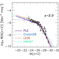
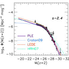
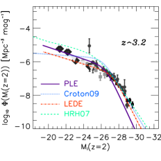
In Fig. 16, we show our best-fit PLE and LEDE models in three redshift bins, and compare our fits to other models that have been presented in the literature.

Croton (2009) presented a modification of the PLE fitting function of Croom et al. (2004) in which the decline of $M_{*}$ with redshift is softened and the bright end power-law slope evolves above $z=3$. This was found to fit the higher redshift SDSS data better than the original fitting form, which was fit only to the 2QZ data. We reproduce this modified fit in Table 8 and Fig. 16, shown by the dotted (blue) line. We see that this model describes the data well at $z\sim 2.0$ and 2.4, but has a too high a normalization and (potentially) too flat a faint-end slope at $z\sim 3.2$.

Hopkins et al. (2007) collected a large set of QLF measurements, from the rest-frame optical, soft and hard X-ray, and mid-IR bands, in order to obtain accurate bolometric corrections and thus determine the bolometric QLF in the redshift interval $z=0-6$. The observational dataset assembled by Hopkins et al. (2007) is impressive, though most of the power in the $z>2$ dataset is from the (R06) optical measurements of the QLF. Taking the traditional double-power law approach, Hopkins et al. (2007) then derive a series of best-fit models to the QLF, including a PLE and luminosity-dependent density evolution (LDDE) model. Their “Full” model, which is an LDDE-based model and includes a luminosity-dependent bolometric correction, is shown in Figure 16 by the (turquoise) dashed lines. This model fits the data well until the highest redshift bin at $z\sim 3.2$. In the Hopkins et al. (2007) model, the break luminosity turns over at $z\sim 2$ and becomes fainter at higher redshift, while the bright end slope flattens and the normalization is constant. This is apparent in Fig. 16, where the break luminosity is clearly much fainter than in our data and the faint end number densities are overpredicted.

Figure 17.— The comparison of our best fit phenomonological models, dashed lines, to the SDSS, BOSS Stripe 82 and boss21+MMT QLF data (points). The number density of various magnitude bins are shown as a function of cosmological time The best-fitting PLE model over $z=0.3-2.2$ and best-fitting LEDE model over $z=2.2-3.5$ from Table 8 are given by the dashed curves. A mismatch in number density at $z=2.2$ for the fainter magnitudes is apparent, but since we do not require the fits to link, is not surprising and within the uncertainties.

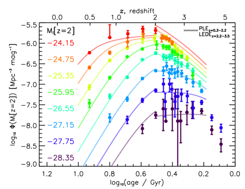
Fig. 17 shows the redshift evolution of the QLF in a series of luminosity bins, including both our data and the best-fit PLE+LEDE model. Previous measurements, especially in the deep X-ray studies (Miyaji et al., 2001; Ueda et al., 2003; Hasinger et al., 2005), and then in the optical by the 2SLAQ QSO survey (Richards et al., 2005; Croom et al., 2009a) see the trend for “AGN Downsizing”, with the number density of fainter AGN peaking at lower-redshift than the luminous AGN. These studies, especially in the optical, have generally suggested that PLE works up to $z\approx 2$, but not to higher $z$. Our BOSS results agree with this statement, but we use the longer redshift baseline of our data, and in particular the fact that we have resolved the break luminosity to $z\sim 3.5$, to find a simple prescription for the evolution at $z>2$. Interestingly, we find that the shape of the QLF does not change (in terms of the power law slopes). Going from high to low redshift there is a build up of quasar activity (the log-linear trend in $\Phi^{*}$) until $z\approx 2$, at which point the number density stalls. In this LEDE-to-PLE toy model scenario, AGN downsizing is then simply a trend in $L^{*}(z)$.

Our optical QLF results are also in general agreement with the latest determination of the hard, 2-10 keV X-ray luminosity function (XLF; Aird et al., 2010). These authors also find an LEDE model (which they name LADE) describe their XLF well, and that an XLF that also retains the same shape, but shifts in luminosity and density, describes the observed evolutionary behavior. We also agree with Aird et al. (2010) in that the (QLF) LEDE model shows a much weaker signature of “AGN Downsizing” than previous studies (Hasinger et al., 2005; Silverman et al., 2008). One caveat here is that the hard X-ray samples used in Aird et al. (2010) are most secure at $z<1.2$. Overall, these trends of a simple log-linear LEDE model describing both the QLF and XLF lends weight to the theory that the X-ray selected AGN population at $z\sim 1$ is a direct descendent of the optical quasar population at $z\sim 2$; a scenario also suggested by quasar and X-ray AGN clustering results (Hickox et al., 2009; Ross et al., 2009; Koutoulidis et al., 2012).

Table 8Values from a set of the best fit double-power law evolution models (e.g. Eqns. 2, 8 and 10). Listed are the redshift ranges of the data fitted, and the best fit values of the model parameters. We perform our fits using only the statistical error on the QLF.

Model	Redshift	$\alpha$	$\beta$	$M_{\rm i}^{*}(z=0)$	$k_{1}$	$k_{2}$	$\log(\Phi^{*})$	$\chi^{2}$/$\nu$
	range	(faint end)	(bright end)				${\rm Mpc}^{-3}{\rm mag}^{-1}$
PLE	0.3–2.2	$-1.16^{+0.02}_{-0.04}$	$-3.37^{+0.03}_{-0.05}$	$-22.85^{+0.05}_{-0.11}$	$1.241^{+0.010}_{-0.028}$	$-0.249^{+0.006}_{-0.017}$	$-5.96^{+0.02}_{-0.06}$	155/75
PLE	1.06–2.2	$-1.23^{+0.06}_{-0.01}$	$-3.55^{+0.06}_{-0.05}$	$-22.92^{+0.24}_{-0.03}$	$1.293^{+0.061}_{-0.014}$	$-0.268^{+0.007}_{-0.031}$	$-6.04^{+0.07}_{-0.02}$	83/52
PLE	2.2–3.5	$-1.52^{+0.05}_{-0.06}$	$-3.10^{+0.15}_{-0.07}$	$-24.29^{+0.26}_{-0.15}$	$1.134^{+0.041}_{-0.047}$	$-0.273^{+0.008}_{-0.006}$	$-6.37^{+0.10}_{-0.06}$	286/113
PLE	0.3–3.5	$-1.34^{+0.06}_{-0.01}$	$-3.56^{+0.08}_{-0.05}$	$-23.04^{+0.15}_{-0.02}$	$1.396^{+0.032}_{-0.009}$	$-0.320^{+0.005}_{-0.004}$	$-6.17^{+0.03}_{-0.01}$	622/195
Crot09	$z<3$	$-1.09$	$-3.31$	$-22.32$	$1.39$	$-0.29$	$-5.78$
Crot09	$z\geq 3$	$-1.09$	$-3.33+0.5(z-3)$	$-22.32$	$1.22$	$-0.23$	$-5.78$
				$M_{\rm i}^{*}(z=2.2)$	$c_{1}$	$c_{2}$
LEDE	2.2–3.5	$-1.42^{+0.51}_{-0.01}$	$-3.53^{+0.09}_{-0.29}$	$-26.70^{+0.22}_{-0.06}$	$-0.604^{+0.005}_{-0.104}$	$-0.678^{+0.216}_{-0.037}$	$-6.08^{+0.39}_{-0.02}$	136/113
LEDE (DR9)	2.2–3.5	$-1.46^{+0.03}_{-0.01}$	$-3.71^{+0.06}_{-0.02}$	$-26.70^{+0.02}_{-0.02}$	$-0.576^{+0.001}_{-0.039}$	$-0.774^{+0.034}_{-0.010}$	$-6.06^{+0.10}_{-0.01}$	1366/107

6.2. Quasar model predictions

There are many models for quasar evolution in the literature, but the modern ones come in three basic flavors. The first implements some of the quasar physics directly into numerical hydrodynamic simulations of galaxy formation or interaction. The second follows much of the same physics semi-analytically. The third tries to relate the properties of quasars and black holes directly to those of dark matter halos or the galaxies which reside in them. We give recent examples from each of these classes of models here.

Figure 18.— The BOSS DR9 Quasar Luminosity Function compared to a series of QLF models from the literature. The model from Conroy & White (2012) is given by the dashed orange line, while the model from Shen (2009) is given by the light-blue dotted line. The Marulli et al. (2008) model is given by the solid turquoise line, the Fanidakis et al. (2012) model by the dot-dashed purple line and the model from (DeGraf et al. 2013) is the shaded black region. We refer the interested reader to the given papers for presentation and discussion of the uncertainties associated with the published models. Left: Measurement in the $1.8<z<2.2$ range; Center: Measurement in the $2.2<z<2.6$ range; Right: Measurement at $z\sim 3.2$. Note, the Shen09 and CW12 models are on top of each other at $M_{i}<-26$.

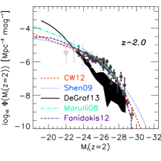
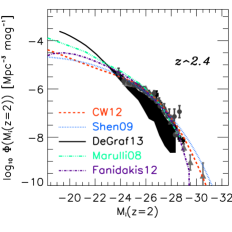
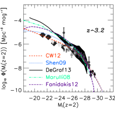
DeGraf et al. (2013, in prep.) present models for the QLF using the new “MassiveBlackII” hydrodynamic simulation, which has a boxsize of 100 $h^{-1}$ Mpc, number of particles, $N_{\rm p}=2\times 1792^{3}$ and a gravitational softening of $\epsilon=1.85$ h^-1 kpc, and employs a WMAP7 (Komatsu et al., 2011) cosmology. These simulations incorporate the physics of hydrodynamics, radiative cooling, star formation, black holes and associated feedback in order to make ab initio predictions for the observed properties of galaxies and quasars. The QLF for each redshift bin is computed using the complete luminosity history of every black hole, producing the best available statistics and extending the predictions to the brightest luminosity by catching rare objects that only occasionally reach very high-$L$. The predictions from these hydrodynamic simulations are given by the shaded black region in Fig. 18. Note that they extend to luminosities fainter than BOSS generally probes.

There are discrepancies between the simulations and the data, especially at $z\approx 2.0$ and 2.4, which may be due to several effects. Previous work on smaller simulations (e.g., Degraf et al., 2010) found that lower resolution simulations produce steeper faint end luminosity functions. Thus increased resolution should further flatten the faint end. At the bright end, volume limitations become significant, with only several black holes reaching the brightest luminosities. The shaded region in the bright end QLF represents an estimate for the cosmic variance using a larger volume simulation (“MassiveBlack”, see DeGraf et al., 2012; Di Matteo et al., 2012). The larger simulation avoids the volume limitations resulting in the upper bound of this region, suggesting that within volume limitations the simulations are consistent with current data.

Marulli et al. (2008) model the cosmological co-evolution of galaxies and their central supermassive black holes within a semi-analytical framework developed on the outputs of the Millennium Simulation (Springel et al., 2005). These authors use the galaxy formation model of Croton et al. (2006) as updated by De Lucia & Blaizot (2007) as their starting point. Luminous quasars in this model occur when a BH accretes cold gas after a major merger of two gas rich galaxies. The accreted mass is proportional to the total cold gas mass present, but with an efficiency which is a function of the size of the system and the merger mass ratio, and chosen to reproduce the observed local $M_{\rm BH}-M_{\rm bulge}$ relation. Marulli et al. (2008) then couple this accretion to various light curve models. The predictions for the luminosity function are shown in Fig. 18 by the triple-dotted-dashed (turquoise) line. We see that this model does well in the lower redshift bins at $z\sim 2.0$ and 2.4 at reproducing the data, but perhaps over predicts the number of faint quasars at $z\sim 3.2$.

For comparison we also consider a second semi-analytic model (Fanidakis et al., 2012). This model is embedded in the semi-analytical galaxy formation code GALFORM (Cole et al., 2000, see also Baugh et al. (2005); Bower et al. (2006)) and predicts the masses, spins (Fanidakis et al., 2011) and mass accretion histories of BHs in tandem with the formation of their host galaxies. In addition to merger-induced triggering they allow triggering when discs becoming dynamically unstable (based on the arguments in Efstathiou et al., 1982). As in Marulli et al. (2008) they also follow quasi-hydrostatic hot gas accretion (known variously as “hot halo mode”, “radio mode” or “radiative mode” accretion) with a rate orders of magnitude below the Eddington limit. The key aspect of the Fanidakis et al. (2012) model in our comparison is that their starburst mode, and thus the BH mass growth, is mainly driven by disc instabilities. Comparison of Marulli et al. (2008) and Fanidakis et al. (2012) thus allows insights into how the triggering mode of quasar activity can potentially be tested by measurements such as ours. The number densities from the Fanidakis et al. (2012) model are calculated considering the entire population of AGN (both obscured and unobscured) and include the empirical obscuration prescription from Hasinger (2008). The QLFs for the unobscured population are shown as (purple) dot-dashed lines in Fig. 18.

Hirschmann et al. (2012) also used semi-analytic models, based on those from Somerville et al. (2008), to examine the properties of accreting BHs and the evolution of the QLF. (We do not show the Hirschmann et al. (2012) predictions in Fig. 18, but their best fitting model fits our data well with potentially a slight overproduction of the faintest QSOs at $z>2.5$; see their Fig. 7.) These authors find that their best fitting model (which includes using “heavy” black hole seeds of $M_{\rm seed}\approx 10^{5-6}M_{\odot}$ at very high $z$ and a varying sub-Eddington limit for the maximum accretion rate at $z\leq 1$) suggests a scenario in which the disc instabilities are the main driver for moderately luminous Seyfert galaxies at low redshift, but major mergers remain the key trigger for luminous AGN/quasars, especially at high $z$.

Shen (2009) presents a phenomenological model for the growth and cosmic evolution of SMBHs, in which the quasar properties are tied to the properties of dark matter halos, rather than galaxies drawn from a semi-analytic model. This model assumes that quasar activity is triggered by major mergers of host halos, and that the resulting light curve follows a universal form, in which its peak luminosity is correlated with the (post)merger halo mass. Quasar activity is quenched at low $z$ and in lower mass halos with phenomenological rules. In particular, the quasar triggering rate depends on a “quasar-on” factor (called $f_{\rm QSO}$ in Shen, 2009) which has exponential cut-offs both at the low and high mass ends which are adjusted to fit the data. These cut-offs ensure that halos with too small a (postmerger) halo mass cannot trigger any quasar activity, while those above a (redshift dependent) maximum mass cannot cool gas efficiently and BH growth halts. With these assumptions, the quasar LF and SMBH growth are tracked self-consistently across cosmic time. The QLF predicted by this model is shown in Fig. 18 by the dotted (blue) line. This model does well at reproducing the data in all three redshift slices, though with a slight over-production of bright quasars at $z\simeq 2.0$.

Recently Conroy & White (2012) presented a model for quasar demographics in which quasars populate galaxies in a simple manner and many of the properties of the quasar population follow naturally from the known, evolving properties of galaxies. A simple “scattered lightbulb” model is adopted, with BHs shining at a fixed fraction of the Eddington luminosity during accretion episodes with Eddington ratios drawn from a lognormal distribution. The quasar duty cycle is explicitly independent of galaxy and BH mass and luminosity, in contrast to the strong dependence invoked in Shen (2009) when connecting quasars to halos. The QLF predictions for that model are shown in Fig. 18 as the (red) dashed lines.

While the models we have highlighted agree with the existing data relatively well, they explain the qualitative behaviors we see in different ways. For example, it is well known that the abundance of bright quasars drops rapidly to low $z$ and that lower mass black hole growth peaks at lower redshift than higher mass black holes (Hasinger et al., 2005; Croom et al., 2009a). In the model of Conroy & White (2012) this is explained through a combination of slow growth of massive galaxies and evolution in the Eddington ratio. In the model of Shen (2009), it involves a suppressing function which simulates the effects of cold gas consumption with time. In the model of Fanidakis et al. (2012) it arises due to a combination of factors, including obscuration evolution.

The models differ significantly in the mass and redshift dependence of the duty cycle, and predict subtle differences in the width of the halo mass distribution at any redshift. In almost all models the characteristic halo mass associated with existing quasar samples is almost independent of redshift. This arises largely due to a chance cancellation of trends in the absolute magnitude limit, the relation between galaxy and halo properties and galaxies, black holes and Eddington ratios.

In the model of Conroy & White (2012), the evolution of the characteristic luminosity is driven by the evolution in the $L-M_{\rm gal}$ and $M_{\rm gal}-M_{h}$ relations, while the break in the LF arises primarily due to the shape of the $M_{\rm gal}-M_{h}$ relation. The Shen (2009) model adjusts the typical host halo of luminous quasars to fit the observed evolution of the break luminosity. In the semi-analytic models, the starburst/quasar mode is powered by one or a combination of major galaxy mergers and disk instabilities with the relative contributions possibly evolving with time. The evolution of the characteristic luminosity thus arises from a complex interplay of factors. Conroy & White (2012) predict that the faint end slope of the LF does not vary significantly, while the bright end slope appears shallower at higher $z$. In the model of Shen (2009), the LF is predicted to turn down at sufficiently low luminosities and high redshifts, since at $z>2$ the minimum Eddington ratio is constrained by the age of the Universe. The hydrodynamic simulations predict a steep faint-end slope at $z\sim 2$. Most of the models have considerable scatter between quasar luminosity and galaxy or halo mass, and thus predict a power-law tail to high luminosity, as observed. Further measurements of this tail at higher $z$ may provide better constraints on this aspect of the models.

In summary, all the models reproduce the QLF and quasar demographics overall reasonably well. We agree with Hirschmann et al. (2012) when they state that further progress on these issues will require data beyond just the luminosity function.

6.3. Discussion

In this final section, we tie our QLF results (and comparisons to models) into the broader context of the link between SMBH growth (see as seen AGN activity) and the properties of galaxies. We take as our starting point the QLF reported here and the clustering measurement and discussion of the BOSS DR9 uniform quasar sample reported in White et al. (2012). Using the same arguments as in White et al. (2012), and the conversions of Croom et al. (2005) and Shen et al. (2009), we place the median BOSS quasar with a bolometric luminosity of $L_{\rm bol}=2-4\times 10^{46}$ erg s^-1, in dark matter haloes of characteristic mass of $\sim 2\times 10^{12}\ h^{-1}M_{\odot}$ at $z\approx 2.5$. Either making the assumption that the BOSS quasars are consistent with the $M_{\rm BH}-M_{\rm halo}$ relation (Ferrarese, 2002; Fine et al., 2006), or, that the quasars radiate at close to the Eddington Limit, $L_{\rm Edd}=10^{47.1}(M_{\rm BH}/10^{9}M_{\odot})$ erg s^-1, suggests that the median $M_{\rm BH}$ in our sample is $\sim 2\times 10^{8}M_{\odot}$. As a guide, a typical $\sim 2\times 10^{8}M_{\odot}$ BH, accreting continuously since $z\sim 2.5$, with an accretion efficiency of $\epsilon=0.1$, and not merging, would have a mass at redshift $z\sim 0$ of $M_{\rm BH}\sim 6\times 10^{10}M_{\odot}$. This would place these objects at the very highest BH masses observed, but also inline with recent results (McConnell et al., 2011). A more realistic scenario, where the duty cycle is $1$%, would lead to $M_{\rm BH}\sim 6\times 10^{8}M_{\odot}$, placing these objects in bulges with $\sigma\sim 250-300$ km s^-1, and thus in early-type galaxies from the relations in e.g. Gültekin et al. (2009).

From the observed clustering (and indeed essentially any of the models quoted above) the typical halo for a BOSS quasar at $z\approx 2.5$ would grow to host a small group by $z\sim 0$. The most likely host galaxy is the central galaxy of the group, since at higher-$z$, any satellites would not be massive enough to host a SMBH. Thus, the typical BOSS quasar host descendant would be the central galaxy of a small group - though we caution that including e.g. the diversity of growth histories of DM halos and scatter in any of the given relations, can easily lead to an order of magnitude dispersion in the above statements (White et al., 2012). Placing these quasars at the centers of groups at $z=0$ is consistent with the suggested velocity dispersions given above. This potentially also suggests that BOSS quasars today are very likely not on the “SF Main Sequence” any more (i.e. they are quenched) even if they were initially. This is also consistent with the recent work by Kelly & Shen (2012).

Leaving the properties of the median BOSS quasar, we now focus on the “extremes” of our population. Taking the most luminous quasars, we find these objects to have close to $\log(L_{\rm bol})=46.0$, and thus black holes in the mass range $\sim 3\times 10^{9}M_{\odot}$ (assuming an Eddington luminosity). At the bright end, the QLF is described by a power-law fall-off, while the massive end of the stellar mass function, the abundance declines exponentially. With a relationship known to exist between $M_{\rm BH}/M_{\rm bulge}$ (and where $M_{\rm bulge}\sim M_{\rm gal}$ for these compact massive galaxies), this argues that there is scatter in $L_{\rm Q}$ at fixed $M_{\rm gal}$. This is perhaps not surprising: at low $z$, $M_{\rm BH}/M_{\rm bulge}$ is measured to have $\sim$0.3 dex in scatter and Eddington ratios are also measured to have $\sim$0.3 dex scatter, so a scatter of at least 0.4 dex overall could be expected. However, this leads to the situation that at high-$L$, scatter is increasingly important, and that bright quasars are “overbright”, and it is currently unclear what underlying physical mechanisms would lead to this enhanced up-scatter. We leave further investigation into the potential evolution of $M_{\rm BH}/M_{\rm gal}$, and the different channels that drives the growth of black holes, the evolution of the number density of quasars, and that of AGN activity in general for future study.

7. Conclusions

The quasar luminosity function is one of the most fundamental observables of this class of important cosmological objects. The shape and evolution of the QLF provides constraints on models of quasar fueling, feedback and galaxy evolution and the ionization history of the inter-galactic gas. Despite its importance, it has proven difficult observationally to probe the quasar luminosity function at magnitudes below the break at the peak of the quasar epoch.

Here we measure the QLF using data from the SDSS-III: Baryon Oscillation Spectroscopic Survey (BOSS) using a uniformly selected sample of 23 301 quasars, and fill in the $L-z$ plane with published results from the SDSS-I/II. We probe the faint end of the QLF to $M_{i}=-24.5$ at $z=2.2$ and complement our uniform color-selection with a sample of variability-selected quasars from the “Stripe 82” field. We also provide a cross-check of our selection function using new, simulated, model, quasar spectra. Amongst our findings are:

• That down to a magnitude limit of $i=21.5$, there are 26.2 and 48.0 quasars deg^-2 across the redshift ranges $2.2<z<3.5$ and $1.0<z<2.2$ respectively. Using the deeper boss21+MMT data, for the unobscured $1.0<z<2.2$ quasar population, there are 78 objects deg^-2 brighter than $i\approx 23.0$, a surface density similar to that selected by a shallow mid-infrared selection (Stern et al., 2012).

• Our combined SDSS+BOSS QLF is reasonably well described by a double power-law, quadratic, pure luminosity evolution (PLE) model across the redshift range $0.3<z<2.2$, with a bright end slope $-3.37^{+0.03}_{-0.05}$, a faint end slope $-1.16^{+0.02}_{-0.04}$, $M^{*}_{i}(z=0)=-22.85^{+0.05}_{-0.11}$, $k_{1}=1.24^{+0.01}_{-0.03}$, $k_{2}=-0.25^{+0.01}_{-0.02}$ and $\log\Phi^{*}=-5.96^{+0.02}_{-0.05}$.

• The simple PLE model breaks down at $z\gtrsim 2.2$. We replace it with a luminosity evolution and density evolution (LEDE) model that has a log-linear trend in both $\Phi^{*}$ and $L^{*}$. This simple form provides a good fit to the data at $2.2<z<3.5$, capturing both the steep decline in number density and the rise in the break luminosity. The data are consistent with no evolution in the power law slopes, though do not strongly constrain the lack of evolution.

• We compare our measured QLF to theoretical models and find a wide variety of models describe our data reasonably well. While the latest hydrodynamic simulations do not fit as well, semi-analytic models in which luminous quasar activity is triggered by major mergers, disk instabilities or a combination of channels can fit our data over a wide range of redshifts. Models based on directly populating halos with quasars can fit the shape of our QLF by assuming a mass and redshift-dependent duty-cycle which is sharply peaked around a characteristic mass. We also find that models which relate black hole mass linearly to galaxy mass and assume a mass-independent duty-cycle match our QLF well.

The results presented here are from the first two, of five, years of BOSS spectroscopy. The upcoming Data Release Ten dataset will cover $\sim 7000\,$deg², include $\sim 150,000$ quasars and will more than double the number in our uniform selection. Future investigations will be able to use this enhanced dataset in order to further quantify, and refine, the selection function for the $2.2<z<3.5$ quasar sample and thus reduce the errors further. This release will include quasars that were observed by BOSS because of their near- and mid-infrared colors, and with these samples we will be able to infer further key properties of quasars at the height of the quasar epoch.

Appendix A Appendix A. Comparison of Quasar Spectral Models

In Section 3.4 we introduced three models for quasar spectral features. In brief, the fiducial model (adopted for our primary analysis) includes a luminosity-dependent emission line template derived from fitting of composite quasar spectra. The composite spectra are created within narrow bins of luminosity, so that mean trends of emission line features with luminosity are reproduced; in particular, the anti-correlation of line equivalent width with continuum luminosity (the “Baldwin Effect”, Baldwin, 1977). Introducing this feature accounts for the luminosity dependence of quasar colors and the effect this has on quasar selection.

For comparison, we include two additional models. The first is based on a fixed emission line template with no luminosity dependence. As this is most similar to models used in previous work (e.g., Richards et al., 2006b; Croom et al., 2009a), it provides a reference point for comparison to QLF estimates that did not include a Baldwin Effect in the selection function estimation. Finally, we also include a model with dust extinction (“exp dust”), motivated by observations of SDSS quasars with mild dust reddening (e.g., Richards et al., 2003; Hopkins et al., 2004).

In Figure 12 we compare the estimated QLFs derived from each of the three selection function models. The systematic effects resulting from imperfect knowledge of the true selection function (or by corollary, the intrinsic distribution of quasar spectral features) is greater than the statistical uncertainties resulting from Poisson variations.

Here, we motivate our choice of selection function (the fiducial model). Our method is a simple qualitative comparison of the observed color-redshift relation for the three models as compared to the data. The method for constructing the color redshift relation is described in Section 3.4.

The resulting relations are shown in Figure 19. The “VdB lines” model does poorly at reproducing the observed colors in the range $2.4\lesssim z\lesssim 3.3$, when Ly$\alpha$ and C IV are in the $g$ and $r$ bands, respectively. The only difference between this model and the fiducial model is the emission line template, thus a model that does not account for the Baldwin Effect will have difficulty reproducing quasar colors at these redshifts. Note that this effect is likely less pronounced in the SDSS data (e.g., Richards et al., 2006b), as it covers less dynamic range in luminosity, and thus most quasars are closer to the mean luminosity represented by a single composite spectrum. The exp dust model appears to do as well as the fiducial model. We chose not to include dust in order to remain more consistent with previous work, and since the focus of this work is on the unobscured quasar population. Unsurprisingly, the exp dust model results in a lower overall completeness, so that the estimated luminosity function is higher overall (Figure 12). We will consider these issues further in subsequent work.

Figure 19.— Color-redshift relations for the three quasar spectral models. Each column of panels represents one of the quasar models named above the top panel. As in Fig. 5, the solid blue lines are the mean and $\pm 1\sigma$ scatter of the colors in redshift bins of $\Delta z=0.05$. The dashed red lines are the same color relations derived from the simulated quasars.

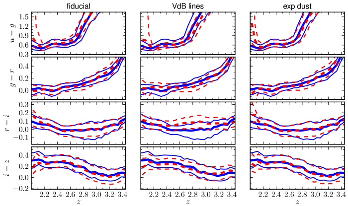
Appendix B Appendix B. Additional BOSS QLF Tables

Here we present additional tables reporting the BOSS QLF for the various samples given in the main text. Table 9 gives the BOSS DR9 QLF as shown in Fig. 13, while Table 10 gives the calculated QLF for the Stripe 82 dataset over the same redshift range and binning (teal points in Fig. 13).

$<z>$	$<M_{i}(z=2)>$	$M_{i}$ bin	$N_{\rm Q}$	$\log(\Phi)$	$\sigma\times 10^{-9}$
2.260	-28.015	-28.050	25	-7.181	9.054
2.256	-27.743	-27.750	29	-7.096	9.985
2.258	-27.431	-27.450	70	-6.836	13.472
2.256	-27.130	-27.150	114	-6.625	17.167
2.257	-26.853	-26.850	203	-6.396	22.356
2.255	-26.544	-26.550	254	-6.273	25.761
2.253	-26.248	-26.250	346	-6.152	29.598
2.255	-25.947	-25.950	473	-5.968	36.587
2.254	-25.653	-25.650	490	-5.868	41.044
2.255	-25.352	-25.350	570	-5.703	49.647

Table 9 The narrowly binned BOSS DR9 Quasar Luminosity Function. The columns are the same as Table 7. The full table appears in the electronic edition of The Astrophysical Journal.

.

$<z>$	$<M_{i}(z=2)>$	$M_{i}$ bin	$N_{\rm Q}$	$\log(\Phi)$	$\sigma\times 10^{-9}$
2.268	-29.762	-29.850	1	-7.898	12.636
2.266	-28.668	-28.650	2	-7.597	17.870
2.246	-28.334	-28.350	2	-7.597	17.870
2.252	-28.080	-28.050	6	-7.120	30.952
2.253	-27.713	-27.750	8	-6.995	35.740
2.244	-27.426	-27.450	7	-7.053	33.432
2.252	-27.150	-27.150	17	-6.668	52.100
2.251	-26.833	-26.850	25	-6.500	63.181
2.253	-26.534	-26.550	37	-6.330	76.863
2.250	-26.247	-26.250	51	-6.191	90.240

Table 10 The narrowly binned BOSS Quasar Luminosity Function using data from 5731 (5476) $2.20<z<4.00\ (3.50)$ quasars selected via their variability signature on Stripe 82 (Sec. 2.4). The columns are the same as Table 7. The full table appears in the electronic edition of The Astrophysical Journal.

.

References

- Abazajian et al. (2005) Abazajian K., et al., 2005, AJ, 129, 1755
- Abazajian et al. (2009) Abazajian K. N., et al., 2009, ApJS, 182, 543
- Adelman-McCarthy et al. (2008) Adelman-McCarthy J. K., et al., 2008, ApJS, 175, 297
- Ahn et al. (2012) Ahn C. P., et al., 2012, ArXiv:1207.7137v1
- Aihara et al. (2011) Aihara H., et al., 2011, The Astrophysical Journal Supplement Series, 193, 29
- Aird et al. (2010) Aird J., et al., 2010, MNRAS, 401, 2531
- Aird et al. (2008) Aird J., Nandra K., Georgakakis A., Laird E. S., Steidel C. C., Sharon C., 2008, MNRAS, 387, 883
- Annis et al. (2011) Annis J., et al., 2011, arXiv:1111.6619v2
- Assef et al. (2011) Assef R. J., et al., 2011, ApJ, 728, 56
- Baldwin (1977) Baldwin J. A., 1977, ApJ, 214, 679
- Barger et al. (2005) Barger A. J., Cowie L. L., Mushotzky R. F., Yang Y., Wang W.-H., Steffen A. T., Capak P., 2005, AJ, 129, 578
- Baugh et al. (2005) Baugh C. M., Lacey C. G., Frenk C. S., Granato G. L., Silva L., Bressan A., Benson A. J., Cole S., 2005, MNRAS, 356, 1191
- Becker et al. (1995) Becker R. H., White R. L., Helfand D. J., 1995, ApJ, 450, 559
- Blanton et al. (2003) Blanton M. R., Lin H., Lupton R. H., Maley F. M., Young N., Zehavi I., Loveday J., 2003, AJ, 125, 2276
- Bolton et al. (2012) Bolton A. S., Schlegel D. J., et al., 2012, ArXiv:1207.7326v1
- Bongiorno et al. (2007) Bongiorno A., et al., 2007, Astron. & Astrophys., 472, 443
- Bovy et al. (2011) Bovy J., et al., 2011, ApJ, 729, 141
- Bower et al. (2006) Bower R. G., Benson A. J., Malbon R., Helly J. C., Frenk C. S., Baugh C. M., Cole S., Lacey C. G., 2006, MNRAS, 370, 645
- Boyle et al. (2000) Boyle B. J., Shanks T., Croom S. M., Smith R. J., Miller L., Loaring N., Heymans C., 2000, MNRAS, 317, 1014
- Boyle et al. (1988) Boyle B. J., Shanks T., Peterson B. A., 1988, MNRAS, 235, 935
- Bramich et al. (2008) Bramich D. M., et al., 2008, MNRAS, 386, 887
- Brandt & Hasinger (2005) Brandt W. N., Hasinger G., 2005, ARA&A, 43, 827
- Brightman & Ueda (2012) Brightman M., Ueda Y., 2012, MNRAS, 423, 702
- Brown et al. (2006) Brown M. J. I., et al., 2006, ApJ, 638, 88
- Burbidge (1967) Burbidge E. M., 1967, ARA&A, 5, 399
- Cattaneo et al. (2009) Cattaneo A., et al., 2009, Nat, 460, 213
- Cole et al. (2000) Cole S., Lacey C. G., Baugh C. M., Frenk C. S., 2000, MNRAS, 319, 168
- Comastri et al. (1995) Comastri A., Setti G., Zamorani G., Hasinger G., 1995, Astron. & Astrophys., 296, 1
- Conroy & White (2012) Conroy C., White M., 2012, arXiv:1208.3198v1
- Corral et al. (2011) Corral A., Della Ceca R., Caccianiga A., Severgnini P., Brunner H., Carrera F. J., Page M. J., Schwope A. D., 2011, Astron. & Astrophys., 530, A42
- Cowie et al. (2003) Cowie L. L., Barger A. J., Bautz M. W., Brandt W. N., Garmire G. P., 2003, ApJ Lett., 584, L57
- Croom et al. (2005) Croom S. M., et al., 2005, MNRAS, 356, 415
- Croom et al. (2009a) Croom S. M., et al., 2009a, MNRAS, 399, 1755
- Croom et al. (2009b) Croom S. M., et al., 2009b, MNRAS, 392, 19
- Croom et al. (2004) Croom S. M., Smith R. J., Boyle B. J., Shanks T., Miller L., Outram P. J., Loaring N. S., 2004, MNRAS, 349, 1397
- Croton (2009) Croton D. J., 2009, MNRAS, 394, 1109
- Croton et al. (2006) Croton D. J., et al., 2006, MNRAS, 365, 11
- Dawson et al. (2012) Dawson K., et al., 2012, ApJS, 999, 999
- De Lucia & Blaizot (2007) De Lucia G., Blaizot J., 2007, MNRAS, 375, 2
- DeGraf et al. (2012) DeGraf C., Di Matteo T., Khandai N., Croft R., Lopez J., Springel V., 2012, MNRAS, 424, 1892
- Degraf et al. (2010) Degraf C., Di Matteo T., Springel V., 2010, MNRAS, 402, 1927
- Di Matteo et al. (2012) Di Matteo T., Khandai N., DeGraf C., Feng Y., Croft R. A. C., Lopez J., Springel V., 2012, ApJ Lett., 745, L29
- Dole et al. (2006) Dole H., et al., 2006, Astron. & Astrophys., 451, 417
- Efstathiou et al. (1982) Efstathiou G., Lake G., Negroponte J., 1982, MNRAS, 199, 1069
- Eisenstein et al. (2011) Eisenstein D. J., Weinberg D. H., et al., 2011, AJ, 142, 72
- Fabian (2012) Fabian A. C., 2012, ARA&A, 50, 455
- Fan (1999) Fan X., 1999, AJ, 117, 2528
- Fan et al. (2006) Fan X., Carilli C. L., Keating B., 2006, ARA&A, 44, 415
- Fan et al. (2001) Fan X., et al., 2001, AJ, 121, 54
- Fan et al. (2004) Fan X., et al., 2004, AJ, 128, 515
- Fan et al. (2006) Fan X., et al., 2006, AJ, 132, 117
- Fanidakis et al. (2011) Fanidakis N., Baugh C. M., Benson A. J., Bower R. G., Cole S., Done C., Frenk C. S., 2011, MNRAS, 410, 53
- Fanidakis et al. (2012) Fanidakis N., et al., 2012, MNRAS, 419, 2797
- Ferrarese (2002) Ferrarese L., 2002, ApJ, 578, 90
- Fine et al. (2006) Fine S., et al., 2006, MNRAS, 373, 613
- Fiore et al. (2012) Fiore F., et al., 2012, Astron. & Astrophys., 537, A16
- Fontanot et al. (2007) Fontanot F., et al., 2007, Astron. & Astrophys., 461, 39
- Francis et al. (1991) Francis P. J., Hewett P. C., Foltz C. B., Chaffee F. H., Weymann R. J., Morris S. L., 1991, ApJ, 373, 465
- Frieman et al. (2008) Frieman J. A., et al., 2008, AJ, 135, 338
- Fukugita et al. (1996) Fukugita M., Ichikawa T., Gunn J. E., Doi M., Shimasaku K., Schneider D. P., 1996, AJ, 111, 1748
- Glikman et al. (2010) Glikman E., Bogosavljević M., Djorgovski S. G., Stern D., Dey A., Jannuzi B. T., Mahabal A., 2010, ApJ, 710, 1498
- Glikman et al. (2011) Glikman E., Djorgovski S. G., Stern D., Dey A., Jannuzi B. T., Lee K., 2011, ApJ Lett., 728, L26+
- Greenstein & Matthews (1963) Greenstein J. L., Matthews T., 1963, Nat, 197, 1041
- Gültekin et al. (2009) Gültekin K., et al., 2009, ApJ, 698, 198
- Gunn et al. (1998) Gunn J. E., et al., 1998, AJ, 116, 3040
- Gunn et al. (2006) Gunn J. E., et al., 2006, AJ, 131, 2332
- Haiman (2012) Haiman Z., 2012, ArXiv e-prints
- Hao et al. (2005) Hao L., et al., 2005, AJ, 129, 1795
- Hasinger (2008) Hasinger G., 2008, ArXiv:0808.0260
- Hasinger et al. (2005) Hasinger G., Miyaji T., Schmidt M., 2005, Astron. & Astrophys., 441, 417
- Hauser & Dwek (2001) Hauser M. G., Dwek E., 2001, ARA&A, 39, 249
- Hazard et al. (1963) Hazard C., Mackey M. B., Shimmins A. J., 1963, Nat, 197, 1037
- Henry (1991) Henry R. C., 1991, ARA&A, 29, 89
- Hickox et al. (2009) Hickox R. C., et al., 2009, ApJ, 696, 891
- Hickox & Markevitch (2006) Hickox R. C., Markevitch M., 2006, ApJ, 645, 95
- Hirschmann et al. (2012) Hirschmann M., Somerville R. S., Naab T., Burkert A., 2012, MNRAS, 426, 237
- Hogg (1999) Hogg D. W., 1999, arXiv:astro-ph/9905116v4
- Hogg et al. (2002) Hogg D. W., et al., 2002, AJ, 124, 646
- Hogg et al. (2001) Hogg D. W., Finkbeiner D. P., Schlegel D. J., Gunn J. E., 2001, AJ, 122, 2129
- Hopkins et al. (2004) Hopkins P. F., et al., 2004, AJ, 128, 1112
- Hopkins et al. (2007) Hopkins P. F., Richards G. T., Hernquist L., 2007, ApJ, 654, 731
- Hunt et al. (2004) Hunt M. P., Steidel C. C., Adelberger K. L., Shapley A. E., 2004, ApJ, 605, 625
- Ikeda et al. (2011) Ikeda H., et al., 2011, ApJ Lett., 728, L25+
- Ikeda et al. (2012) Ikeda H., et al., 2012, ApJ
- Ivezić et al. (2004) Ivezić Ž., et al., 2004, Astronomische Nachrichten, 325, 583
- Ivezić et al. (2007) Ivezić Ž., et al., 2007, AJ, 134, 973
- Jakobsen et al. (1994) Jakobsen P., Boksenberg A., Deharveng J. M., Greenfield P., Jedrzejewski R., Paresce F., 1994, Nat, 370, 35
- Jannuzi & Dey (1999) Jannuzi B. T., Dey A., 1999, in Weymann R., et al. eds, ASP Conf. Ser. 191: Photometric Redshifts and the Detection of High Redshift Galaxies p. 111
- Jiang et al. (2006) Jiang L., et al., 2006, AJ, 131, 2788
- Jiang et al. (2008) Jiang L., et al., 2008, AJ, 135, 1057
- Jiang et al. (2009) Jiang L., et al., 2009, AJ, 138, 305
- Jiang et al. (2007) Jiang L., Fan X., Ivezić Ž., Richards G. T., Schneider D. P., Strauss M. A., Kelly B. C., 2007, ApJ, 656, 680
- Kelly & Shen (2012) Kelly B. C., Shen Y., 2012, arXiv:1209.0477v1
- Kimball et al. (2011) Kimball A. E., Ivezić Ž., Wiita P. J., Schneider D. P., 2011, AJ, 141, 182
- Kirkpatrick et al. (2011) Kirkpatrick J. A., et al., 2011, ApJ, in prep.
- Komatsu et al. (2011) Komatsu E., et al., 2011, ApJS, 192, 18
- Koutoulidis et al. (2012) Koutoulidis L., Plionis M., Georgantopoulos I., Fanidakis N., 2012, arXiv:1209.6460v1
- Lacy et al. (2004) Lacy M., et al., 2004, ApJS, 154, 166
- Lehmer et al. (2012) Lehmer B. D., et al., 2012, ApJ, 752, 46
- Lonsdale et al. (2003) Lonsdale C. J., et al., 2003, PASP, 115, 897
- Luo et al. (2011) Luo B., et al., 2011, ApJ, 740, 37
- Lupton et al. (2001) Lupton R., Gunn J. E., Ivezić Z., Knapp G. R., Kent S., 2001, in F. R. Harnden Jr., F. A. Primini, & H. E. Payne ed., Astronomical Data Analysis Software and Systems X Vol. 238 of Astronomical Society of the Pacific Conference Series, The SDSS Imaging Pipelines. p. 269
- Lynden-Bell (1969) Lynden-Bell D., 1969, Nat, 223, 690
- Lynds (1971) Lynds R., 1971, ApJ Lett., 164, L73+
- MacLeod et al. (2011) MacLeod C. L., et al., 2011, ApJ, 728, 26
- Madau & Rees (2001) Madau P., Rees M. J., 2001, ApJ Lett., 551, L27
- Martin et al. (2005) Martin D. C., et al., 2005, ApJ Lett., 619, L1
- Marulli et al. (2008) Marulli F., Bonoli S., Branchini E., Moscardini L., Springel V., 2008, MNRAS, 385, 1846
- Masters et al. (2012) Masters D., et al., 2012, ApJ
- McConnell et al. (2011) McConnell N. J., Ma C.-P., Gebhardt K., Wright S. A., Murphy J. D., Lauer T. R., Graham J. R., Richstone D. O., 2011, Nat, 480, 215
- McDonald & Eisenstein (2007) McDonald P., Eisenstein D. J., 2007, Phys. Rev. D, 76, 063009
- McGreer et al. (2009) McGreer I. D., Helfand D. J., White R. L., 2009, AJ, 138, 1925
- McQuinn & White (2011) McQuinn M., White M., 2011, MNRAS, 415, 2257
- Meiksin (2009) Meiksin A. A., 2009, Reviews of Modern Physics, 81, 1405
- Miyaji et al. (2001) Miyaji T., Hasinger G., Schmidt M., 2001, Astron. & Astrophys., 369, 49
- Morrissey et al. (2007) Morrissey P., et al., 2007, ApJS, 173, 682
- Myers et al. (2003) Myers A. D., Outram P. J., Shanks T., Boyle B. J., Croom S. M., Loaring N. S., Miller L., Smith R. J., 2003, MNRAS, 342, 467
- Netzer & Trakhtenbrot (2007) Netzer H., Trakhtenbrot B., 2007, ApJ, 654, 754
- Oke (1963) Oke J. B., 1963, Nat, 197, 1040
- Oke & Gunn (1983) Oke J. B., Gunn J. E., 1983, ApJ, 266, 713
- Oke & Sandage (1968) Oke J. B., Sandage A., 1968, ApJ, 154, 21
- Osmer (1982) Osmer P. S., 1982, ApJ, 253, 28
- Padmanabhan et al. (2008) Padmanabhan N., et al., 2008, ApJ, 674, 1217
- Page & Carrera (2000) Page M. J., Carrera F. J., 2000, MNRAS, 311, 433
- Palanque-Delabrouille et al. (2011) Palanque-Delabrouille N., et al., 2011, Astron. & Astrophys., 530, A122
- Palanque-Delabrouille et al. (2012) Palanque-Delabrouille N., et al., 2012, arXiv:1209.3968v1
- Pâris et al. (2012) Pâris I. P., et al., 2012, arXiv:1210.5166v1
- Peebles (1980) Peebles P. J. E., 1980, The Large-Scale Structure of the Universe. Princeton University Press, 1980.
- Peebles (1993) Peebles P. J. E., 1993, Principles of Physical Cosmology. Princeton, NJ: Princeton University Press
- Pier et al. (2003) Pier J. R., Munn J. A., Hindsley R. B., Hennessy G. S., Kent S. M., Lupton R. H., Ivezić Ž., 2003, AJ, 125, 1559
- Prevot et al. (1984) Prevot M. L., Lequeux J., Prevot L., Maurice E., Rocca-Volmerange B., 1984, Astron. & Astrophys., 132, 389
- Rees (1984) Rees M. J., 1984, ARA&A, 22, 471
- Reimers et al. (2005) Reimers D., Fechner C., Hagen H.-J., Jakobsen P., Tytler D., Kirkman D., 2005, Astron. & Astrophys., 442, 63
- Reimers et al. (1997) Reimers D., Kohler S., Wisotzki L., Groote D., Rodriguez-Pascual P., Wamsteker W., 1997, Astron. & Astrophys., 327, 890
- Reyes et al. (2008) Reyes R., et al., 2008, AJ, 136, 2373
- Richards et al. (2001a) Richards G. T., et al., 2001a, AJ, 121, 2308
- Richards et al. (2001b) Richards G. T., et al., 2001b, AJ, 122, 1151
- Richards et al. (2002) Richards G. T., et al., 2002, AJ, 123, 2945
- Richards et al. (2003) Richards G. T., et al., 2003, AJ, 126, 1131
- Richards et al. (2005) Richards G. T., et al., 2005, MNRAS, 360, 839
- Richards et al. (2006a) Richards G. T., et al., 2006a, ApJS, 166, 470
- Richards et al. (2006b) Richards G. T., et al., 2006b, AJ, 131, 2766
- Richards et al. (2009) Richards G. T., et al., 2009, ApJS, 180, 67
- Richstone & Schmidt (1980) Richstone D. O., Schmidt M., 1980, ApJ, 235, 361
- Ross et al. (2009) Ross N. P., et al., 2009, ApJ, 697, 1634
- Ross et al. (2012) Ross N. P., et al., 2012, ApJS, 199, 3
- Salpeter (1964) Salpeter E. E., 1964, ApJ, 140, 796
- Sandage (1961) Sandage A. R., 1961, Sky & Telescope, 21, 148
- Schlegel et al. (1998) Schlegel D. J., Finkbeiner D. P., Davis M., 1998, ApJ, 500, 525
- Schmidt et al. (2010) Schmidt K. B., Marshall P. J., Rix H.-W., Jester S., Hennawi J. F., Dobler G., 2010, ApJ, 714, 1194
- Schmidt (1963) Schmidt M., 1963, Nat, 197, 1040
- Schmidt (1970) Schmidt M., 1970, ApJ, 162, 371
- Schmidt et al. (1995) Schmidt M., Schneider D. P., Gunn J. E., 1995, AJ, 110, 68
- Schneider et al. (2005) Schneider D. P., et al., 2005, AJ, 130, 367
- Schneider et al. (2010) Schneider D. P., et al., 2010, AJ, 139, 2360
- Scoville et al. (2007a) Scoville N., et al., 2007a, ApJS, 172, 38
- Scoville et al. (2007b) Scoville N., et al., 2007b, ApJS, 172, 1
- Scranton et al. (2002) Scranton R., et al., 2002, ApJ, 579, 48
- Sesar et al. (2007) Sesar B., et al., 2007, AJ, 134, 2236
- Shang et al. (2005) Shang Z., et al., 2005, ApJ, 619, 41
- Shang et al. (2011) Shang Z., et al., 2011, ApJS, 196, 2
- Shankar et al. (2010) Shankar F., Crocce M., Miralda-Escudé J., Fosalba P., Weinberg D. H., 2010, ApJ, 718, 231
- Shankar et al. (2009) Shankar F., Weinberg D. H., Miralda-Escudé J., 2009, ApJ, 690, 20
- Shanks et al. (1991) Shanks T., Georgantopoulos I., Stewart G. C., Pounds K. A., Boyle B. J., Griffiths R. E., 1991, Nat, 353, 315
- Shen (2009) Shen Y., 2009, ApJ, 704, 89
- Shen et al. (2009) Shen Y., et al., 2009, ApJ, 697, 1656
- Shen & Kelly (2012) Shen Y., Kelly B. C., 2012, ApJ, 746, 169
- Siana et al. (2008) Siana B., et al., 2008, ApJ, 675, 49
- Silverman et al. (2005) Silverman J. D., et al., 2005, ApJ, 624, 630
- Silverman et al. (2008) Silverman J. D., et al., 2008, ApJ, 679, 118
- Singal et al. (2011) Singal J., Petrosian V., Lawrence A., Stawarz Ł., 2011, ApJ, 743, 104
- Singal et al. (2012) Singal J., Petrosian V., Stawarz L., Lawrence A., 2012, arXiv:1207.3396v1
- Slosar et al. (2011) Slosar A., et al., 2011, LABEL:@jnlJ. Cosmology Astropart. Phys., 9, 1
- Smee et al. (2012) Smee S., et al., 2012, AJ, 999, 999
- Smette et al. (2002) Smette A., Heap S. R., Williger G. M., Tripp T. M., Jenkins E. B., Songaila A., 2002, ApJ, 564, 542
- Smith et al. (2002) Smith J. A., et al., 2002, AJ, 123, 2121
- Soltan (1982) Soltan A., 1982, MNRAS, 200, 115
- Somerville et al. (2008) Somerville R. S., Hopkins P. F., Cox T. J., Robertson B. E., Hernquist L., 2008, MNRAS, 391, 481
- Springel et al. (2005) Springel V., et al., 2005, Nat, 435, 629
- Stern et al. (2012) Stern D., et al., 2012, arXiv:1205.0811v1
- Stoughton et al. (2002) Stoughton C., et al., 2002, AJ, 123, 485
- Swanson et al. (2008) Swanson M. E. C., Tegmark M., Blanton M., Zehavi I., 2008, MNRAS, 385, 1635
- Syphers et al. (2011) Syphers D., Anderson S. F., Zheng W., Meiksin A., Haggard D., Schneider D. P., York D. G., 2011, ApJ, 726, 111
- Tegmark et al. (2004) Tegmark M., et al., 2004, ApJ, 606, 702
- Telfer et al. (2002) Telfer R. C., Zheng W., Kriss G. A., Davidsen A. F., 2002, ApJ, 565, 773
- Tepper-García (2006) Tepper-García T., 2006, MNRAS, 369, 2025
- Treister et al. (2009) Treister E., Urry C. M., Virani S., 2009, ApJ, 696, 110
- Tucker et al. (2006) Tucker D. L., et al., 2006, Astronomische Nachrichten, 327, 821
- Tueller et al. (2010) Tueller J., et al., 2010, ApJS, 186, 378
- Ueda et al. (2003) Ueda Y., Akiyama M., Ohta K., Miyaji T., 2003, ApJ, 598, 886
- Vanden Berk et al. (2001) Vanden Berk D. E., et al., 2001, AJ, 122, 549
- Vestergaard & Wilkes (2001) Vestergaard M., Wilkes B. J., 2001, ApJS, 134, 1
- Volonteri et al. (2003) Volonteri M., Haardt F., Madau P., 2003, ApJ, 582, 559
- Volonteri et al. (2005) Volonteri M., Madau P., Quataert E., Rees M. J., 2005, ApJ, 620, 69
- Volonteri & Rees (2006) Volonteri M., Rees M. J., 2006, ApJ, 650, 669
- Warren et al. (1994) Warren S. J., Hewett P. C., Osmer P. S., 1994, ApJ, 421, 412
- White et al. (2011) White M., et al., 2011, ApJ, 728, 126
- White et al. (2012) White M., et al., 2012, MNRAS, 999, 126
- White et al. (2003) White R. L., Becker R. H., Fan X., Strauss M. A., 2003, AJ, 126, 1
- Willott et al. (2009) Willott C. J., et al., 2009, AJ, 137, 3541
- Willott et al. (2010) Willott C. J., et al., 2010, AJ, 139, 906
- Wittman et al. (2002) Wittman D. M., et al., 2002, in J. A. Tyson & S. Wolff ed., Society of Photo-Optical Instrumentation Engineers (SPIE) Conference Series Vol. 4836 of Presented at the Society of Photo-Optical Instrumentation Engineers (SPIE) Conference, Deep lens survey. pp 73–82
- Wolf et al. (2003) Wolf C., Wisotzki L., Borch A., Dye S., Kleinheinrich M., Meisenheimer K., 2003, Astron. & Astrophys., 408, 499
- Worseck et al. (2011) Worseck G., et al., 2011, ApJ Lett., 733, L24
- Worseck & Prochaska (2011) Worseck G., Prochaska J. X., 2011, ApJ, 728, 23
- Wright (2006) Wright E. L., 2006, PASP, 118, 1711
- Wu et al. (2009) Wu J., Vanden Berk D. E., Brandt W. N., Schneider D. P., Gibson R. R., Wu J., 2009, ApJ, 702, 767
- Yan et al. (2012) Yan L., et al., 2012, arXiv:1209.2065v1
- York et al. (2000) York D. G., et al., 2000, AJ, 120, 1579
- Zel’dovich & Novikov (1965) Zel’dovich Y. B., Novikov I. D., 1965, Soviet Physics Doklady, 9, 834