Cross-Entropy Clustering

Abstract

We build a general and highly applicable clustering theory, which we call cross-entropy clustering (shortly CEC) which joins advantages of classical k-means (easy implementation and speed) with those of EM (affine invariance and ability to adapt to clusters of desired shapes). Moreover, contrary to k-means and EM, CEC finds the optimal number of clusters by automatically removing groups which carry no information.

Although CEC, similarly like EM, can be build on an arbitrary family of densities, in the most important case of Gaussian CEC the division into clusters is affine invariant, while the numerical complexity is comparable to that of k-means.

1 Introduction

1.1 Motivation

As is well-known, clustering plays a basic role in many parts of data engineering, pattern recognition and image analysis [1, 2, 3, 4, 5]. Thus it is not surprising that there are many methods of data clustering, many of which however inherit the deficiencies of the first method called k-means [6, 7]. Since k-means has the tendency to divide the data into spherical shaped clusters of similar sizes, it is not affine invariant and does deal well with clusters of various sizes. This causes the so-called mouse-effect, see Figure 1(b). Moreover, it does not find the right number of clusters, see 1(c), and consequently to apply it we usually need to use additional tools like gap statistics [8, 9].

(a) Mouse-like set.

(b) k-means with $k=3$.

(c) k-means with $k=10$.

(d) Spherical CEC.

Figure 1: Clustering of the uniform density on mouse-like set (Fig. 1(a)) by standard k-means algorithm with $k=3$ (Fig. 1(b)) and $k=10$ (Fig. 1(c)) compared with Spherical CEC (Fig. 1(d)) with initially $10$ clusters (finished with $3$).

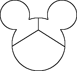
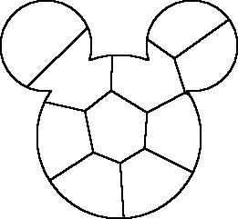
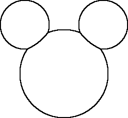
Since k-means has so many disadvantages, one can ask why it is so popular. One of the possible answers lies in the fact that k-means is simple to implement and very fast comparing to more advanced clustering methods like EM and classification EM [10, 11].

So let us now discuss EM, the other end approach to clustering. It is based on family of densities $\mathcal{F}$ which convex combination we allow to estimate the density of the data-set we study. By modifying $\mathcal{F}$ we can adapt our method to the search of clusters of various types [12]. The disadvantages follow from the fact that EM is relatively slow and not well-adapted to dealing with large data-sets. Let us also add that EM, analogously as k-means, does not find the right number of clusters.

In our paper we construct a general cross-entropy clustering (CEC) theory which simultaneously joins, and even overcomes, the clustering advantages of classical k-means and EM. The aim of this paper is to study the theoretical background of cross-entropy clustering. Due to its length we decided to illustrate it only on basic examples.

1.2 Main idea

We based CEC on the observation that it is often profitable to use various compression algorithms specialized in different data types. We apply this observation in reverse, namely we group/cluster those data together which are compressed by one algorithm from the preselected set of compressing algorithms. In development of this idea we were influenced by the classical Shannon Entropy Theory [16, 17, 18, 19] and Minimum Description Length Principle [20, 21]. In particular we were strongly inspired by the application of MDLP to image segmentation given in [22, 23].

From theoretical point of view our basic idea lies in applying cross-entropy to many “compressing” densities. Its greatest advantage is the automatic reduction of unnecessary clusters: contrary to the case of classical k-means or EM, there is a memory cost of using each cluster. Consequently from cross-entropy clustering point of view it is in many cases profitable to decrease the number of used clusters.

Example 1.1.

(a) Four gaussians.

(b) 4 clusters

(c) Bear-like set.

(d) 6 clusters.

Figure 2: Gaussian CEC starting from $10$ initial clusters.

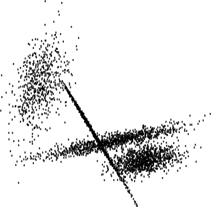
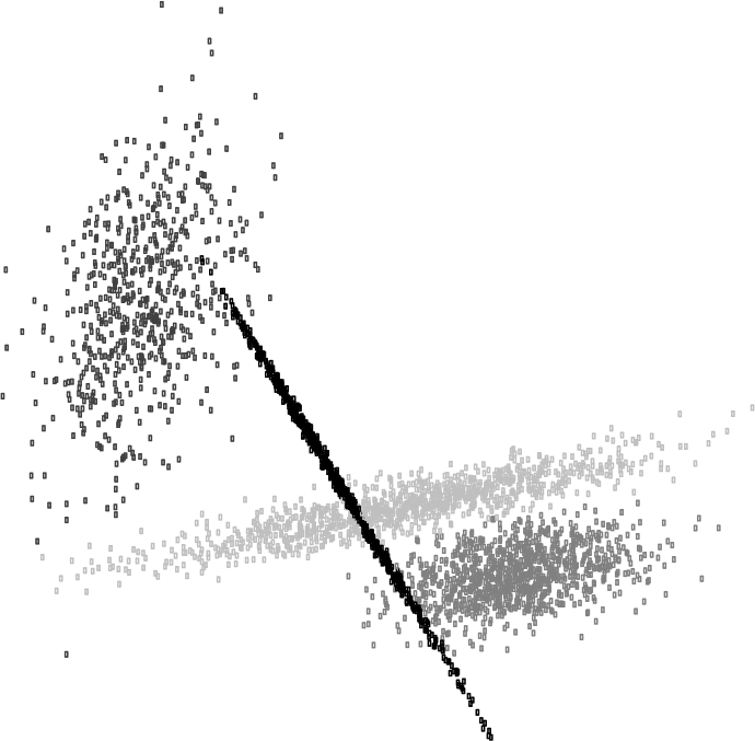
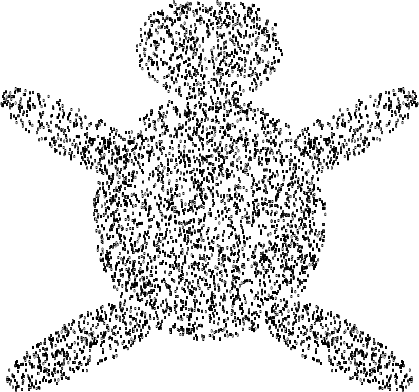
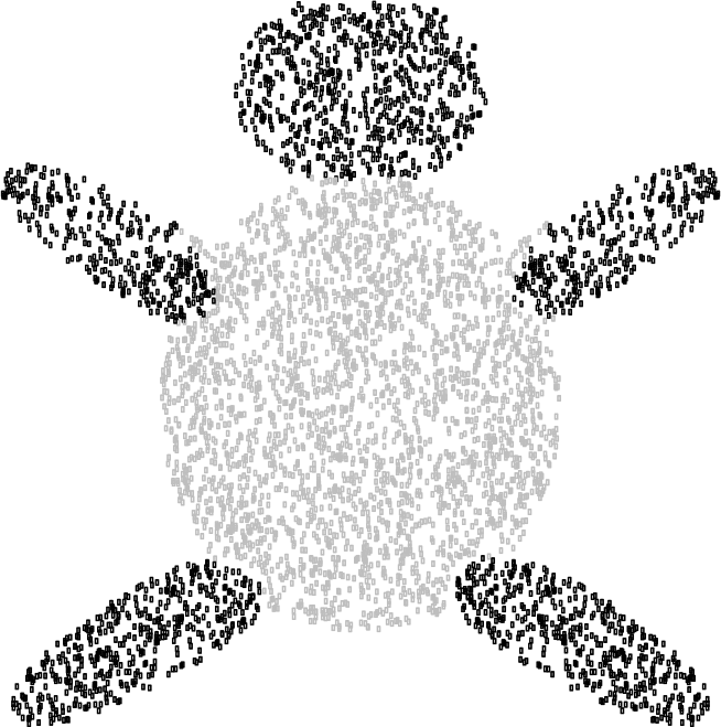
To visualize our theory let us look at the results of Gaussian CEC given in Figure 2. In both cases we started with $k=10$ initial randomly chosen clusters which were reduced automatically by the algorithm.

In practical implementations our approach can viewed as a generalized and “modified” version of the classical k-means clustering As a consequence the complexity of the CEC is usually that of k-means and one can easily adapt most ideas used in various versions of k-means to CEC.

Since CEC is in many aspects influenced by EM let us briefly summarize the main similarities and differences. Suppose that we are given a continuous probability measure $\mu$ (which represents our data) with density $f_{\mu}$ and fixed densities $f_{1},\ldots,f_{k}$ by combination of which we want to approximate $f_{\mu}$.

• The basic goal of EM is to find probabilities $p_{1},\ldots,p_{k}$ such that the approximation

  $$f_{\mu}\approx p_{1}f_{1}+\ldots+p_{k}f_{k}$$ (1.1)

  is optimal.

• In CEC we search for partition of $\mathbb{R}^{N}$ into (possibly empty) pairwise disjoint sets $U_{1},\ldots,U_{k}$ and probabilities $p_{1},\ldots,p_{k}$ such that the approximation

  $$f_{\mu}\approx p_{1}f_{1}|_{U_{1}}\cup\ldots\cup p_{k}f_{k}|_{U_{k}}$$ (1.2)

  is optimal.

Observe that as a result of CEC we naturally obtain the partition of the space into sets $(U_{i})_{i=1}^{k}$. Another crucial consequence of the formula (1.2) is that contrary to the earlier approaches based on MLE we approximate $f_{\mu}$ not by a density, as is the case in (1.1), but subdensity.

1.3 Contents of the paper

For the convenience of the reader we now briefly summarize the contents of the article. In the following section we discuss (mostly) known results concerning entropy which we will need in our study. In particular we identify the subdensities with coding/compressing algorithms. In the third section we provide a detailed motivation and explanation of our basic idea, which allows to interpret the cross-entropy for the case of many “coding densities”. More precisely, given a partition $U_{1},\ldots,U_{k}$ of $\mathbb{R}^{N}$ and subdensity families $\mathcal{F}_{1},\ldots,\mathcal{F}_{k}$, we introduce the subdensity family $\operatorname*{\uplus}\limits_{i=1}^{k}(\mathcal{F}_{i}|U_{i})$, which consists of those acceptable codings in which elements of $U_{i}$ are compressed by a fixed element from $\mathcal{F}_{i}$. We also show how to apply classical Lloyds and Hartigan approaches to cross-entropy minimizations.

The last section contains applications of our theory to clustering. We first consider a general idea of cross-entropy $\mathcal{F}$-clustering, which aim is to find a $\mu$-partition $(U_{i})_{i=1}^{k}$ minimizing

$$H^{\times}\!\big{(}\mu\|\operatorname*{\uplus}_{i=1}^{k}(\mathcal{F}|{U_{i}})\big{)}.$$

This allows to investigate the $\mathcal{F}$-divergence of the $\mu$-partition $(U_{i})_{i=1}^{k}$

$$d_{\mu}(\mathcal{F};(U_{i})_{i=1}^{k}):=H^{\times}\!\big{(}\mu\|\mathcal{F}\big{)}-H^{\times}\!\big{(}\mu\|\operatorname*{\uplus}_{i=1}^{k}(\mathcal{F}|{U_{i}})\big{)}$$

which measures the validity of the clustering $(U_{i})_{i=1}^{k}$.

Next we proceed to the study of clustering with respect to various Gaussian subfamilies. First we investigate the most important case of Gaussian CEC and show that it reduces to the search for the partition $(U_{i})_{i=1}^{k}$ of the given data-set $U$ for which the value of

$$\sum_{i=1}^{k}p(U_{i})\cdot[-\ln(p(U_{i}))+\frac{1}{2}\ln\mathrm{det}(\Sigma_{U_{i}})]$$

is minimal, where $p(V)=\mathrm{card}(V)/\mathrm{card}(U)$ and $\Sigma_{V}$ denotes the covariance matrix of the set $V$. It occurs that the Gaussian clustering is affine invariant.

Then we study clustering based on the Spherical Gaussians, that is those with covariance proportional to identity. Comparing Spherical CEC to classical k-means we obtain that: clustering is scale and translation invariant and clusters do not tend to be of fixed size. Consequently we do not obtain the mouse effect

Example 1.2.

Let us observe on Figure 1 the comparison of Spherical CEC with classical k-means on the Mickey-Mouse-like set. We see that Spherical CEC was able to find the “right” number of clusters, and that the clusters have “reasonable” shapes.

To apply Spherical clustering we need the same information as in the classical k-means: in the case of k-means we seek the splitting of the data $U\subset\mathbb{R}^{N}$ into $k$ sets $(U_{i})_{i=1}^{k}$ such that the value of $\sum\limits_{i=1}^{k}p(U_{i})\cdot D_{U_{i}}$ is minimal, where $D_{V}=\frac{1}{\mathrm{card}(V)}\sum\limits_{v\in V}\|v-\mathrm{m}_{V}\|^{2}$ denotes the mean within cluster $V$ sum of squares (and $\mathrm{m}_{V}$ is the mean of $V$). It occurs that the Gaussian spherical clustering in $\mathbb{R}^{N}$ reduces to minimization of

$$\sum\limits_{i=1}^{k}p(U_{i})\cdot[-\ln(p(U_{i}))+\frac{N}{2}\ln D_{U_{i}}].$$

Next we proceed to the study of clustering by Gaussians with fixed covariance. We show that in the case of bounded data the optimal amount of clusters is bounded above by the maximal cardinality of respective $\varepsilon$-net in the convex hull of the data. We finish our paper with the study of clustering by Gaussian densities with covariance equal to $s\mathrm{I}$ and prove that with $s$ converging to zero we obtain the classical k-means clustering, while with $s$ growing to $\infty$ data will form one big group.

2 Cross-entropy

2.1 Compression and cross-entropy

Since CEC is based on choosing the optimal (from the memory point of view) coding algorithms, we first establish notation and present the basics of cross-entropy compression.

Assume that we are given a discrete probability distribution $\nu$ on a finite set $X=\{x_{1},\ldots,x_{k}\}$ which attains the values $x_{i}$ with probabilities $f_{i}$. Then roughly speaking [16] the optimal code-lengths in the case we use coding alphabet consisting of $d$ symbols to code $\nu$ are given by $l_{i}=-\log_{d}f_{i}$, and consequently the expected code length is given by the entropy

$$\begin{array}[]{l}h_{d}(\nu):=\sum\limits_{i=1}^{k}f_{i}l_{i}=\sum\limits_{i=1}^{k}f_{i}\cdot(-\log_{d}f_{i})=\frac{1}{\ln d}\sum\limits_{i=1}^{k}\mathrm{sh}(f_{i}),\end{array}$$

where $\mathrm{sh}(x)$ denotes the Shannon function defined by $-x\cdot\ln x$ if $x>0$ and $\mathrm{sh}(0):=0$. We recall that for arbitrary code-lengths $l_{i}$ to be acceptable they have to satisfy Kraft’s inequality $\sum\limits_{i=1}^{k}d^{-l_{i}}\leq 1$.

If we code a discrete probability measure $\mu$ (which attains $x_{i}$ with probability $g_{i}$) by the code optimized for a subprobabilistic measure $\nu$ we arrive at the definition of cross-entropy $h_{d}^{\times}(\mu\|f)$, which is given as the expected code length

$$h_{d}^{\times}(\mu\|f):=\sum_{i=1}^{k}g_{i}\cdot(-\log_{d}f_{i}).$$

Let us proceed to the case of continuous probability measure $\nu$ on $\mathbb{R}^{N}$ (with density $f_{\nu}$). The role of entropy is played by differential entropy (which corresponds to the limiting value of discrete entropy of coding with quantization error going to zero [16]):

$$h_{d}(\nu):=\int f_{\nu}(x)\cdot(-\log_{d}f_{\nu}(x))dx=\frac{1}{\ln d}\int\mathrm{sh}(f_{\nu}(x))dx,$$

where $f_{\nu}$ denotes the density of the measure $\nu$. In fact, as was the case of discrete spaces, we will need to consider codings produced by subprobability measures.

Definition 2.1.

We call a nonnegative measurable function $f:\mathbb{R}^{N}\to\mathbb{R}_{+}$ a subdensity if $\int_{\mathbb{R}^{N}}f(x)dx\leq 1$.

Thus the differential code-length connected with subdensity $f$ is given by

$$l(x)=-\log_{d}f(x).$$ (2.1)

Dually, an arbitrary measurable function $x\to l(x)$ is acceptable as a “differential coding length” if it satisfies the differential version of the Kraft’s inequality:

$$\int d^{-l(x)}dx\leq 1,$$ (2.2)

which is equivalent to saying that the function $f(x):=d^{-l(x)}$ is a subdensity.

From now on, if not otherwise specified, by $\mu$ we denote either continuous or discrete probability measure on $\mathbb{R}^{N}$.

Definition 2.2.

We define the cross-entropy of $\mu$ with respect to subdensity $f$ by:

$$H_{d}^{\times}(\mu\|f):=\int-\log_{d}f(y)d\mu(y).$$ (2.3)

It is well-known that if $\mu$ has density $f_{\mu}$, the minimum in the above integral over all subdensities is obtained for $f=f_{\mu}$ (and consequently the cross-entropy is bounded from below by the differential entropy).

One can easily get the following:

Observation 2.1.

Let $f$ be a given subdensity and $A$ an invertible affine operation. Then

$$H^{\times}_{d}(\mu\circ A^{-1}\|f_{A})=H^{\times}_{d}(\mu\|f)+\log_{d}|\mathrm{det}A|,$$

where $f_{A}$ is a subdensity defined by

$$f_{A}:x\to f(A^{-1}x)/|\mathrm{det}A|,$$ (2.4)

and $\mathrm{det}A$ denotes the determinant of the linear component of $A$.

In our investigations we will be interested in (optimal) coding for $\mu$ by elements of a set of subdensities $\mathcal{F}$, and therefore we put

$$H_{d}^{\times}(\mu\|\mathcal{F}):=\inf\{H_{d}^{\times}(\mu\|f):f\in\mathcal{F}\}.$$

One can easily check that if $\mathcal{F}$ consists of densities then the search for $H^{\times}(\mu\|\mathcal{F})$ reduces to the maximum likelihood estimation of measure $\mu$ by the family $\mathcal{F}$. Thus by $\mathrm{MLE}(\mu\|\mathcal{F})$ we will denote the set of all subdensities from $\mathcal{F}$ which realize the infimum:

$$\mathrm{MLE}(\mu\|\mathcal{F}):=\{f\in\mathcal{F}:H_{d}^{\times}(\mu\|f)=H_{d}^{\times}(\mu\|\mathcal{F})\}.$$

In proving that the clustering is invariant with respect to the affine transformation $A$ we will use the following simple corollary of Observation 2.1:

Corollary 2.1.

Let $\mathcal{F}$ be the subdensity family and $A:\mathbb{R}^{N}\to\mathbb{R}^{N}$ an invertible affine operation. By $\mathcal{F}_{A}$ we denote $\{f_{A}:f\in\mathcal{F}\}$, where $f_{A}$ is defined by (2.4). Then

$$H_{d}^{\times}(\mu\circ A^{-1}\|\mathcal{F}_{A})=H_{d}^{\times}(\mu\|\mathcal{F})+\log_{d}|\mathrm{det}A|.$$ (2.5)

As we know entropy in the case when we code with $d$ symbols is a rescaling of entropy computed in Nats, which can be symbolically written as: $H_{d}(\cdot)=\frac{1}{\ln d}H_{e}(\cdot)$. Consequently, for the shortness of notation when we compute the entropy in Nats we will omit the subscript $e$ in the entropy symbol

$$H^{\times}(\cdot):=H_{e}^{\times}(\cdot).$$

2.2 Cross-entropy for Gaussian families

By $\mathrm{m}_{\mu}$ and $\Sigma_{\mu}$ we denote the mean and covariance of the measure $\mu$, that is

$$\begin{array}[]{l}\mathrm{m}_{\mu}=\frac{1}{\mu(\mathbb{R}^{N})}\int x\,d\mu(x),\\[4.30554pt] \Sigma_{\mu}=\frac{1}{\mu(\mathbb{R}^{N})}\int(x-\mathrm{m}_{\mu})(x-\mathrm{m}_{\mu})^{T}\,d\mu(x).\end{array}$$

For measure $\mu$ and measurable set $U$ such that $0<\mu(U)<\infty$ we introduce the probability measure $\mu_{U}$

$$\mu_{U}(A):=\mbox{$\frac{1}{\mu(U)}$}\mu(A\cap U),$$

and use the abbreviations

$$\begin{array}[]{l}\mathrm{m}_{U}^{\mu}:=\mathrm{m}_{\mu_{U}}=\frac{1}{\mu(U)}\int_{U}x\,d\mu(x),\\[4.30554pt] \Sigma_{U}^{\mu}:=\Sigma_{\mu_{U}}=\frac{1}{\mu(U)}\int_{U}(x-\mathrm{m}_{\mu})(x-\mathrm{m}_{\mu})^{T}\,d\mu(x).\end{array}$$

The basic role in Gaussian cross-entropy minimization is played by the following result which says that we can reduce computation to gaussian families. Since its proof is essentially known part of MLE, we provide here only its short idea.

Given symmetric positive matrix $\Sigma$, we recall that by the Mahalanobis distance [25, 26] we understand

$$\|x-y\|_{\Sigma}:=(x-y)^{T}\Sigma^{-1}(x-y).$$

By $\mathcal{N}\!{(\mathrm{m},\Sigma)}$ we denote the normal density with mean $\mathrm{m}$ and covariance $\Sigma$, which as we recall is given by the formula

$$\mathcal{N}\!{(\mathrm{m},\Sigma)}(x):=\frac{1}{\sqrt{(2\pi)^{N}\mathrm{det}(\Sigma)}}\exp(\mbox{$\frac{1}{2}$}\|x-\mu\|_{\Sigma}^{2}).$$

Theorem 2.1.

Let $\mu$ be a discrete or continuous probability measure with well-defined covariance matrix, and let $\mathrm{m}\in\mathbb{R}^{N}$ and positive-definite symmetric matrix $\Sigma$ be given.

Then

$$H^{\times}\!\big{(}\mu\|\mathcal{N}\!{(\mathrm{m},\Sigma)}\big{)}=H^{\times}\big{(}\mu_{\mathcal{G}}\|\mathcal{N}\!{(\mathrm{m},\Sigma)}\big{)},$$

where $\mu_{\mathcal{G}}$ denotes the probability measure with Gaussian density of the same mean and covariance as $\mu$ (that is the density of $\mu_{\mathcal{G}}$ equals $\mathcal{N}\!(\mathrm{m}_{\mu},\Sigma_{\mu})$).

Consequently

$$H^{\times}\!\big{(}\mu\|\mathcal{N}\!{(\mathrm{m},\Sigma)}\big{)}=\frac{N}{2}\ln(2\pi)+\frac{1}{2}\|\mathrm{m}-\mathrm{m}_{\mu}\|^{2}_{\Sigma}+\frac{1}{2}\mathrm{tr}(\Sigma^{-1}\Sigma_{\mu})+\frac{1}{2}\ln\mathrm{det}(\Sigma).$$ (2.6)

Sketch of the proof.

We consider the case when $\mu$ is a continuous measure with density $f_{\mu}$. One can easily see that by applying trivial affine transformations and (2.5) it is sufficient to prove (2.6) in the case when $\mathrm{m}=0$ and $\Sigma=\mathrm{I}$. Then we have

$$\begin{array}[]{l}H^{\times}(\mu\|\mathcal{N}\!{(0,\mathrm{I})})=\int f_{\mu}(x)\cdot[\frac{N}{2}\ln(2\pi)+\frac{1}{2}\ln\mathrm{det}(\mathrm{I})+\frac{1}{2}\|x\|^{2}]dx\\[4.30554pt] =\frac{N}{2}\ln(2\pi)+\frac{1}{2}\int f_{\mu}(x)\|(x-\mathrm{m}_{\mu})+\mathrm{m}_{\mu}\|^{2}dx\\[4.30554pt] =\frac{N}{2}\ln(2\pi)+\!\frac{1}{2}\int\!f_{\mu}(x)[\|x-\mathrm{m}_{\mu}\|^{2}\!+\|\mathrm{m}_{\mu}\|^{2}\!+2(x-\mathrm{m}_{\mu})\circ\mathrm{m}_{\mu}]dx\\[4.30554pt] =\frac{N}{2}\ln(2\pi)+\frac{1}{2}\mathrm{tr}(\Sigma_{\mu})+\frac{1}{2}\|\mathrm{m}_{\mu}\|^{2}.\end{array}$$

∎

By $\mathcal{G}$ we denote the set of all normal densities, while by $\mathcal{G}_{\Sigma}$ we denote the set of all normal densities with covariance $\Sigma$. As a trivial consequence of the Theorem 2.1 we obtain the following proposition.

Proposition 2.1.

Let $\Sigma$ be a fixed positive symmetric matrix. Then $\mathrm{MLE}(\mu\|\mathcal{G}_{\Sigma})=\{\mathcal{N}\!{(\mathrm{m}_{\mu},\Sigma)}\}$ and $H^{\times}(\mu\|\mathcal{G}_{\Sigma})=\frac{N}{2}\ln(2\pi)+\frac{1}{2}\mathrm{tr}(\Sigma^{-1}\Sigma_{\mu})+\frac{1}{2}\ln\mathrm{det}(\Sigma)$.

Now we consider cross-entropy with respect to all normal densities.

Proposition 2.2.

We have $\mathrm{MLE}(\mu\|\mathcal{G})=\{\mathcal{N}\!{(\mathrm{m}_{\mu},\Sigma_{\mu})}\}$ and

$$H^{\times}(\mu\|\mathcal{G})=\frac{1}{2}\ln\mathrm{det}(\Sigma_{\mu})+\frac{N}{2}\ln(2\pi e).$$ (2.7)

Proof.

Since entropy is minimal when we code a measure by its own density, we easily obtain that

$$H^{\times}(\mu\|\mathcal{G})=H^{\times}(\mu_{\mathcal{G}}\|\mathcal{G})=H^{\times}(\mu_{\mathcal{G}}\|\mathcal{N}\!(\mathrm{m}_{\mu},\Sigma_{\mu}))$$

$$=H(\mu_{\mathcal{G}})=\frac{1}{2}\ln\mathrm{det}(\Sigma_{\mu})+\frac{N}{2}\ln(2\pi e).$$

Consequently the minimum is realized for $\mathcal{N}\!{(\mathrm{m}_{\mu},\Sigma_{\mu})}$. ∎

Due to their importance and simplicity we also consider Spherical Gaussians $\mathcal{G}_{(\cdot\mathrm{I})}$, that is those with covariance matrix proportional to $\mathrm{I}$:

$$\mathcal{G}_{(\cdot\mathrm{I})}=\bigcup_{s>0}\mathcal{G}_{s\mathrm{I}}.$$

We will need the denotation for the mean squared distance from the mean

$$D_{\mu}:=\int\|x-\mathrm{m}_{\mu}\|^{2}d\mu(x)=\mathrm{tr}(\Sigma_{\mu}),$$

which will play in Spherical Gaussians the analogue of covariance. As is the case for the covariance, we will use the abbreviation

$$D_{U}^{\mu}:=D_{\mu_{U}}=\frac{1}{\mu(U)}\int_{U}\|x-\mathrm{m}^{\mu}_{U}\|^{2}d\mu(x).$$

Observe, that if $\Sigma_{\mu}=s\mathrm{I}$ then $D_{\mu}=Ns$. In the case of one dimensional measures $\sqrt{D_{\mu}}$ is exactly the standard deviation of the measure $\mu$. It occurs that $D_{\mu}$ can be naturally interpreted as a square of the “mean radius” of the measure $\mu$: for the uniform probability measure $\mu$ on the sphere $S(x,R)\subset\mathbb{R}^{N}$ we clearly get $\sqrt{D_{\mu}}=R$. Moreover, as we show in the following observation $\sqrt{D_{\mu}}$ will be close to $R$ even for the uniform probability distribution on the ball $B(x,R)$.

By $\lambda$ we denote the Lebesgue measure on $\mathbb{R}^{N}$. Recall that according to our notation $\lambda_{U}$ denotes the probability measure defined by $\lambda_{U}(A):=\lambda(A\cap U)/\lambda(U)$.

Observation 2.2.

We put $V_{n}:=\lambda(B_{n}(0,1))=\pi^{n/2}/\Gamma(n/2+1)$, where $B_{n}(0,1)$ denotes the unit ball in $\mathbb{R}^{n}$.

Consider the unit ball $B(0,1)\subset\mathbb{R}^{N}$. Directly from the definition of covariance we get $\Sigma_{B(0,1)}^{\lambda}=c_{N}\mathrm{I}$, where

$$\begin{array}[]{l}c_{N}=\frac{1}{V_{N}}\int\limits_{-1}^{1}x^{2}V_{N-1}\cdot(\sqrt{1-x^{2}})^{N-1}dx\\ =\frac{\Gamma(N/2+1)}{\sqrt{\pi}\Gamma((N-1)/2+1)}\int\limits_{-1}^{1}x^{2}(1-x^{2})^{(N-1)/2}dx=\frac{1}{N+2}.\end{array}$$

Consequently,

$$\begin{array}[]{l}\Sigma^{\lambda}_{B(x,R)}=R^{2}\Sigma^{\lambda}_{B(0,1)}=\frac{R^{2}}{N+2},\\[4.30554pt] D^{\lambda}_{B(x,R)}=\mathrm{tr}(\Sigma^{\lambda}_{B(x,R)})=\frac{NR^{2}}{N+2},\end{array}$$ (2.8)

and therefore $\sqrt{D^{\lambda}_{B(x,R)}}=\sqrt{\frac{N}{N+2}}\cdot R\to R\mbox{ as }N\to\infty$.

Proposition 2.3.

We have $\mathrm{MLE}(\mu\|\mathcal{G}_{(\cdot\mathrm{I})})=\{\mathcal{N}\!(\mathrm{m}_{\mu},\frac{D_{\mu}}{N}\mathrm{I})\}$ and

$$H^{\times}(\mu\|\mathcal{G}_{(\cdot\mathrm{I})})=\frac{N}{2}\ln(D_{\mu})+\frac{N}{2}\ln(2\pi e/N).$$ (2.9)

Proof.

Clearly by Proposition 2.1

$$H^{\times}(\mu\|\mathcal{G}_{(\cdot\mathrm{I})})=\inf_{s>0}H^{\times}(\mu\|\mathcal{G}_{s\mathrm{I}})=\inf_{s>0}\left(\frac{1}{2s}D_{\mu}+\frac{N}{2}\ln s+\frac{N}{2}\ln(2\pi)\right).$$

Now by easy calculations we obtain that the above function attains minimum for $s=D_{\mu}/N$ and equals the RHS of (2.9). ∎

At the end we consider the cross-entropy with respect to $\mathcal{G}_{s\mathrm{I}}$ (spherical Gaussians with fixed scale). As a direct consequence of Proposition 2.1 we get:

Proposition 2.4.

Let $s>0$ be given. Then $\mathrm{MLE}(\mu\|\mathcal{G}_{s\mathrm{I}})=\{\mathcal{N}\!(\mathrm{m}_{\mu},s\mathrm{I})\}$ and

$$H^{\times}(\mu\|\mathcal{G}_{s\mathrm{I}})=\frac{1}{2s}D_{\mu}+\frac{N}{2}\ln s+\frac{N}{2}\ln(2\pi).$$

3 Many coding subdensities

3.1 Basic idea

In the previous section we considered the coding with $d$-symbols of the $\mu$-randomly chosen point $x\in\mathbb{R}^{N}$ by the code optimized for the subdensity $f$. Since it is often better to “pack/compress” parts of data with various algorithms, we follow this approach and assume that we are given a sequence of $k$ subdensities $(f_{i})_{i=1}^{k}$, which we interpret as coding algorithms.

Suppose that we want to code $x$ by $j$-th algorithm from the sequence $(f_{i})_{i=1}^{k}$. By (2.1) the length of code of $x$ corresponds to $-\log_{d}f_{j}(x)$. However, this code itself is clearly insufficient to decode $x$ if we do not know which coding algorithm was used. Therefore to uniquely code $x$ we have to add to it the code of $j$. Thus if $l_{j}$ denotes the length of code of $j$, the “final” length of the code of the point $x$ is the sum of $l_{j}$ and the length of the code of the point $x$:

$$\mbox{code-length of }x=l_{j}-\log_{d}f_{j}(x).$$

Since the coding of the algorithms has to be acceptable, the sequence $(l_{i})_{i=1}^{k}$ has to satisfy the Kraft’s inequality and therefore if we put $p_{i}=d^{-l_{i}}$, we can consider only those $p_{i}\geq 0$ that $\sum\limits_{i=1}^{k}p_{i}\leq 1$. Consequently without loss of generality (by possibly shortening the expected code-length), we may restrict to the case when $\sum\limits_{i=1}^{k}p_{i}=1$.

Now suppose that points from $U_{i}\subset\mathbb{R}^{N}$ we code by the subdensity $f_{i}$. Observe that although $U_{i}$ have to be pairwise disjoint, they do not have to cover the whole space $\mathbb{R}^{N}$ – we can clearly omit the set with $\mu$-measure zero. To formalize this, the notion of $\mu$-partition for a given continuous or discrete measure $\mu$ is convenient: we say that a pairwise disjoint sequence $(U_{i})_{i=1}^{k}$ of Lebesgue measurable subsets of $\mathbb{R}^{N}$ is a $\mu$-partition if

$$\mu\left(\mathbb{R}^{N}\setminus\bigcup_{i=1}^{k}U_{i}\right)=0.$$

To sum up: we have the “coding” subdensities $(f_{i})_{i=1}^{k}$ and $p\in P_{k}$, where

$$P_{k}:=\{(p_{1},\ldots,p_{k})\in[0,1]^{k}:\sum_{i=1}^{k}p_{i}=1\}.$$

As $U_{i}$ we take the set of points of $\mathbb{R}^{N}$ we code by density $f_{i}$. Then for a $\mu$-partition $(U_{i})_{i=1}^{k}$ we obtain the code-length function

$$x\to-\log_{d}p_{i}-\log_{d}f_{i}(x)\mbox{ for }x\in U_{i},$$

which is exactly the code-length of the subdensity

$$p_{1}f_{1}|_{U_{1}}\cup\ldots\cup p_{k}f_{k}|_{U_{k}}.$$ (3.1)

In general we search for those $p$ and $\mu$-partition for which the expected code-length given by the cross-entropy $H^{\times}\!\big{(}\mu\|\operatorname*{\cup}\limits_{i=1}^{k}p_{i}f_{i}|_{U_{i}}\big{)}$ will be minimal.

Definition 3.1.

Let $(\mathcal{F}_{i})_{i=1}^{k}$ be a sequence of subdensity families in $\mathbb{R}^{N}$, and let a $\mu$-partition $(U_{i})_{i=1}^{k}$ be given. Then we define

$$\operatorname*{\uplus}\limits_{i=1}^{k}(\mathcal{F}_{i}|U_{i}):=\big{\{}\operatorname*{\cup}\limits_{i=1}^{k}p_{i}f_{i}|_{U_{i}}:(p_{i})_{i=1}^{k}\in P_{k},(f_{i})_{i=1}^{k}\in(\mathcal{F}_{i})_{i=1}^{k}\big{\}}.$$

Observe that $\operatorname*{\uplus}\limits_{i=1}^{k}(\mathcal{F}_{i}|U_{i})$ denotes those compression algorithms which can be build by using an arbitrary compression subdensity from $\mathcal{F}_{i}$ on the set $U_{i}$.

3.2 Lloyd’s algorithm

The basic aim of our article is to find a $\mu$-partition $(U_{i})_{i=1}^{k}$ for which

$$H^{\times}_{d}\!\big{(}\mu\,\|\,\operatorname*{\uplus}\limits_{i=1}^{k}(\mathcal{F}_{i}|U_{i})\big{)}$$

is minimal. In general it is NP-hard problem even for k-means [27], which is the simplest limiting case of Spherical CEC (see Observation 4.7). However, in practice we can often hope to find a sufficiently good solution by applying either Lloyd’s or Hartigan’s method.

The basis of Lloyd’s approach is given by the following two results which show that

• given $p\in P_{k}$ and $(f_{i})_{i=1}^{k}\in(\mathcal{F}_{i})_{i=1}^{k}$, we can find a partition $(U_{i})_{i=1}^{k}$ which minimizes the cross-entropy $H^{\times}\!\big{(}\mu\|\operatorname*{\cup}\limits_{i=1}^{k}p_{i}f_{i}|_{U_{i}}\big{)}$;

• for a partition $(U_{i})_{i=1}^{k}$, we can find $p\in P_{k}$ and $(f_{i})_{i=1}^{k}\in(\mathcal{F}_{i})_{i=1}^{k}$ which minimizes $H^{\times}\!\big{(}\mu\|\operatorname*{\cup}\limits_{i=1}^{k}p_{i}f_{i}|_{U_{i}}\big{)}$.

We first show how to minimize the value of cross-entropy being given a $\mu$-partition $(U_{i})_{i=1}^{k}$. From now on we interpret $0\cdot x$ as zero even if $x=\pm\infty$ or $x$ is not properly defined.

Observation 3.1.

Let $(f_{i})\in(\mathcal{F}_{i})$, $p\in P_{k}$ and $(U_{i})_{i=1}^{k}$ be a $\mu$-partition. Then

$$H^{\times}\!\big{(}\mu\|\operatorname*{\cup}\limits_{i=1}^{k}p_{i}f_{i}|_{U_{i}}\big{)}=\sum\limits_{i=1}^{k}\mu(U_{i})\cdot\left(-\ln p_{i}+H^{\times}(\mu_{U_{i}}\|f_{i})\right).$$ (3.2)

Proof.

We have

$$\begin{array}[]{rcl}H^{\times}\!\big{(}\mu\|\operatorname*{\cup}\limits_{i=1}^{k}p_{i}f_{i}|_{U_{i}}\big{)}&=&\sum\limits_{i=1}^{k}\int_{U_{i}}-\ln p_{i}-\log_{d}f_{i}(x)d\mu(x)\\[2.15277pt] &=&\sum\limits_{i=1}^{k}\mu(U_{i})\cdot\left(-\ln p_{i}-\int\ln(f_{i}(x))d\mu_{U_{i}}(x)\right).\end{array}$$

∎

Proposition 3.1.

Let the sequence of subdensity families $(\mathcal{F}_{i})_{i=1}^{k}$ be given and let $(U_{i})_{i=1}^{k}$ be a fixed $\mu$-partition. We put $p=(\mu(U_{i}))_{i=1}^{k}\in P_{k}$.

Then

$$H^{\times}\!\big{(}\mu\|\operatorname*{\uplus}_{i=1}^{k}(\mathcal{F}_{i}|U_{i})\big{)}=H^{\times}\!\big{(}\mu\|\operatorname*{\cup}\limits_{i=1}^{k}p_{i}f_{i}|_{U_{i}}\big{)}$$

$$=\sum_{i=1}^{k}\mu(U_{i})\cdot[-\ln(\mu(U_{i})+H^{\times}(\mu_{U_{i}}\|\mathcal{F}_{i})].$$

Proof.

We apply the formula (3.2)

$$H^{\times}\!\big{(}\mu\|\operatorname*{\cup}\limits_{i=1}^{k}\tilde{p}_{i}f_{i}|_{U_{i}}\big{)}=\sum\limits_{i=1}^{k}\mu(U_{i})\cdot\left(-\ln\tilde{p}_{i}+H^{\times}(\mu_{U_{i}}\|f_{i})\right).$$

By the property of classical entropy we know that the function

$$P_{k}\ni\tilde{p}=(\tilde{p}_{i})_{i=1}^{k}\to\sum\limits_{i=1}^{k}\mu(U_{i})\cdot(-\ln\tilde{p}_{i})$$

is minimized for $\tilde{p}=(\mu(U_{i}))_{i}$. ∎

The above can be equivalently rewritten with the use of notation:

$$h_{\mu}(\mathcal{F};W):=\begin{cases}\mu(W)\!\cdot\!\big{(}-\ln(\mu(W))+H^{\times}(\mu_{W}\|\mathcal{F})\big{)}\mbox{ if }\mu(W)>0,\\ 0\mbox{ otherwise.}\end{cases}$$

Thus $h_{\mu}(\mathcal{F};W)$ tells us what is the minimal cost of compression of the part of our dataset contained in $W$ by subdensities from $\mathcal{F}$. By Proposition 3.1 if $(U_{i})_{i=1}^{k}$ is a $\mu$-partition then

$$H^{\times}\!\big{(}\mu\|\operatorname*{\uplus}_{i=1}^{k}(\mathcal{F}_{i}|U_{i})\big{)}=\sum_{i=1}^{k}h_{\mu}(\mathcal{F}_{i};U_{i}).$$ (3.3)

Observe that, in general, if $\mu(U)>0$ then

$$H^{\times}(\mu_{U}\|\mathcal{F})=\ln(\mu(U))+\frac{1}{\mu(U)}h_{\mu}(\mathcal{F};U).$$

Consequently, if we are given a $\mu_{U}$-partition $(U_{i})_{i=1}^{k}$, then

$$H^{\times}(\mu_{U}\|\operatorname*{\uplus}\limits_{i=1}^{k}(\mathcal{F}_{i}|U_{i}))=\ln(\mu(U))+\frac{1}{\mu(U)}\sum\limits_{i=1}^{k}h_{\mu}(\mathcal{F}_{i};U_{i}).$$

Theorem 3.1.

Let the sequence of subdensity families $(\mathcal{F}_{i})_{i=1}^{k}$ be given and let $(U_{i})_{i=1}^{k}$ be a fixed $\mu$-partition.

We put $p=(\mu(U_{i}))_{i=1}^{k}\in P_{k}$. We assume that $\mathrm{MLE}(\mu_{U_{i}}\|\mathcal{F}_{i})$ is nonempty for every $i=1..k$. Then for arbitrary

$$f_{i}\in\mathrm{MLE}(\mu_{U_{i}}\|\mathcal{F}_{i})\mbox{ for }i=1,\ldots,k,$$ (3.4)

we get

$$H^{\times}\!\big{(}\mu\|\operatorname*{\uplus}_{i=1}^{k}(\mathcal{F}_{i}|U_{i})\big{)}=H^{\times}\!\big{(}\mu\|\operatorname*{\uplus}_{i=1}^{k}p_{i}f_{i}|_{U_{i}}\big{)}.$$

Proof.

Directly from the definition of $\mathrm{MLE}$ we obtain that

$$H^{\times}(\mu_{U_{i}}\|\tilde{f}_{i})\geq H^{\times}(\mu_{U_{i}}\|\mathcal{F}_{i})=H^{\times}(\mu_{U_{i}}\|f_{i})$$

for $\tilde{f}_{i}\in\mathcal{F}_{i}$. ∎

The following theorem is a dual version of Theorem 3.1 – for fixed $p\in P_{k}$ and $f_{i}\in\mathcal{F}_{i}$ we seek optimal $\mu$-partition which minimizes the cross-entropy.

By the support of measure $\mu$ we denote the support of its density if $\mu$ is continuous and the set of support points if it is discrete.

Theorem 3.2.

Let the sequence of subdensity families $(\mathcal{F}_{i})_{i=1}^{k}$ be given and let $f_{i}\in\mathcal{F}_{i}$ and $p\in P_{k}$ be such that $\mathrm{supp}(\mu)\subset\bigcup\limits_{i=1}^{k}\mathrm{supp}(f_{i})$. We define $l:\mathrm{supp}(\mu)\to(-\infty,\infty]$ by

$$l(x):=\min\limits_{i\in\{1,\ldots,k\}}[-\ln p_{i}-\ln f_{i}(x)].$$

We construct a sequence $(U_{i})_{i=1}^{k}$ of measurable subsets of $\mathbb{R}^{N}$ recursively by the following procedure:

• $U_{1}=\{x\in\mathrm{supp}(\mu):-\ln p_{1}-\ln f_{1}(x)=l(x)\}$;

• $U_{l+1}=\{x\in\mathrm{supp}(\mu)\setminus(U_{1}\cup\ldots\cup U_{l}):-\ln p_{l+1}-\ln f_{l+1}(x)=l(x)\}$.

Then $(U_{i})_{i=1}^{k}$ is a $\mu$-partition and

$$H^{\times}\!\big{(}\mu\|\operatorname*{\cup}\limits_{i=1}^{k}p_{i}f_{i}|_{U_{i}}\big{)}=\inf\{H^{\times}\!\big{(}\mu\|\operatorname*{\cup}\limits_{i=1}^{k}p_{i}f_{i}|_{V_{i}}\big{)}:\mbox{$\mu$-partition }(V_{i})_{i=1}^{k}\}.$$

Proof.

Since $\mathrm{supp}(\mu)\subset\bigcup\limits_{i=1}^{k}\mathrm{supp}(f_{i})$, we obtain that $(U_{i})_{i=1}^{k}$ is a $\mu$-partition. Moreover, directly by the choice of $(U_{i})_{i=1}^{k}$ we obtain that

$$\begin{array}[]{l}l(x)=\ln(\operatorname*{\cup}\limits_{i=1}^{k}p_{i}f_{i}|_{U_{i}})(x)\mbox{ for }x\in\mathrm{supp}(\mu),\end{array}$$

and consequently for an arbitrary $\mu$-partition $(V_{i})_{i=1}^{k}$ we get

$$\begin{array}[]{l}H^{\times}(\mu\|\operatorname*{\cup}\limits_{i=1}^{k}p_{i}f_{i}|_{V_{i}})=\int\operatorname*{\cup}\limits_{i=1}^{k}\big{[}-\ln(p_{i})-\ln(f_{i}|_{V_{i}}(x))\big{]}d\mu(x)\\[2.15277pt] \leq\int\bar{l}(x)d\mu(x)=\int\operatorname*{\cup}\limits_{i=1}^{k}\big{[}-\ln(p_{i})-\ln(f_{i}|_{U_{i}}(x))\big{]}d\mu(x).\end{array}$$

∎

As we have mentioned before, Lloyd’s approach is based on alternate use of steps from Theorems 3.1 and 3.2. In practice we usually start by choosing initial densities and set probabilities $p_{k}$ equal: $p=(1/k,\ldots,1/k)$ (since the convergence is to local minimum we commonly start from various initial condition several times).

Observe that directly by Theorems 3.1 and 3.2 we obtain that the sequence $n\to h_{n}$ is decreasing. One hopes that limit $h_{n}$ converges (or at least is reasonably close) to the global infimum of $H^{\times}\!\big{(}\mu\|\operatorname*{\uplus}\limits_{i=1}^{k}(\mathcal{F}_{i}|U_{i})\big{)}$.

To show a simple example of cross-entropy minimization we first need some notation. We are going to discuss the Lloyds cross-entropy minimization of discrete data with respect to $\mathcal{G}_{\Sigma_{1}},\ldots,\mathcal{G}_{\Sigma_{K}}$. As a direct consequence of (3.3) and Proposition 2.1 we obtain the formula for the cross entropy of $\mu$ with respect to a family of Gaussians with covariances $(\Sigma_{i})_{i=1}^{k}$.

Observation 3.2.

Let $(\Sigma_{i})_{i=1}^{k}$ be fixed positive symmetric matrices and let $(U_{i})_{i=1}^{k}$ be a given $\mu$-partition. Then

$$\begin{array}[]{l}H^{\times}(\mu\|\operatorname*{\uplus}\limits_{i=1}^{k}(\mathcal{G}_{\Sigma_{i}}|U_{i}))=\\[4.30554pt] \frac{N}{2}\ln(2\pi)+\sum\limits_{i=1}^{k}\mu(U_{i})\big{[}\!-\ln(\mu(U_{i}))+\frac{1}{2}\mathrm{tr}(\Sigma_{i}^{-1}\Sigma^{\mu}_{U_{i}})+\frac{1}{2}\ln\mathrm{det}(\Sigma_{i})\big{]}.\end{array}$$

Example 3.1.

(a) $T$-like set.

(b) Partition into two groups.

Figure 3: Effect of clustering by Lloyd’s algorithm on $T$-like shape.

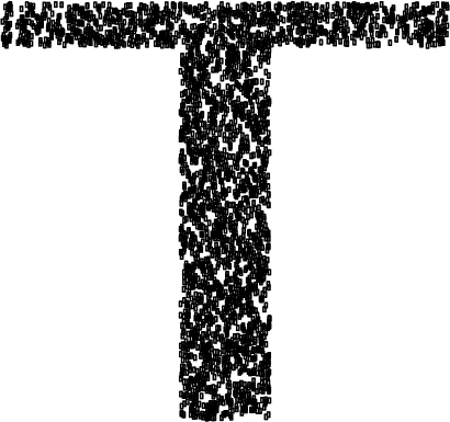
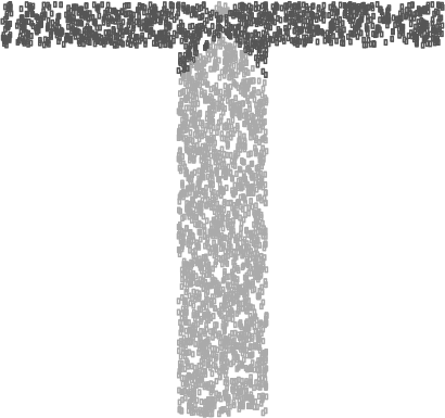
We show Lloyd’s approach to cross-entropy minimization of the set $\mathrm{Y}$ showed on Figure 3(a). As is usual, we first associate with the data-set $\mathrm{Y}$ the probability measure defined by the formula

$$\mu:=\frac{1}{\mathrm{card}\mathrm{Y}}\sum_{y\in\mathrm{Y}}\delta_{y},$$

where $\delta_{y}$ denotes the Dirac delta at the point $y$.

Next we search for the $\mu$-partition $\mathrm{Y}=\mathrm{Y}_{1}\sqcup\mathrm{Y}_{2}$ which minimizes

$$H^{\times}\!\big{(}\mu\|(\mathcal{G}_{\Sigma_{1}}|\mathrm{Y}_{1})\uplus(\mathcal{G}_{\Sigma_{2}}|\mathrm{Y}_{2})\big{)},$$

where $\Sigma_{1}=[300,0;0,1]$, $\Sigma_{2}=[1,0;0,300]$. The result is given on Figure 3(b), where the dark gray points which belong to $\mathrm{Y}_{1}$ are “coded” by density from $\mathcal{G}_{\Sigma_{1}}$ and light gray belonging to $\mathrm{Y}_{2}$ and are “coded” by density from $\mathcal{G}_{\Sigma_{2}}$.

3.3 Hartigan algorithm

Due to its nature to use Hartigan we have to divide the data-set (or more precisely the support of the measure $\mu$) into “basic parts/blocks” from which we construct our clustering/grouping. Suppose that we have a fixed $\mu$-partition $\mathcal{V}=(V_{i})_{i=1}^{n}$. The aim of Hartigan is to find such $\mu$-partition build from elements of $\mathcal{V}$ which has minimal cross-entropy.

Consider $k$ coding subdensity families $(\mathcal{F}_{i})_{i=1}^{k}$. To explain Hartigan approach more precisely we need the notion of group membership function $\mathrm{gr}:\{1,\ldots,n\}\to\{0,\ldots,k\}$ which describes the membership of $i$-th element of partition, where $0$ value is a special symbol which denotes that $V_{i}$ is as yet unassigned. In other words: if $\mathrm{gr}(i)=l>0$, then $V_{i}$ is a part of the $l$-th group, and if $\mathrm{gr}(i)=0$ then $V_{i}$ is unassigned.

We want to find such $\mathrm{gr}:\{1,\ldots,n\}\to\{1,\ldots,k\}$ (thus all elements of $\mathcal{V}$ are assigned) that

$$\sum_{i=1}^{k}h_{\mu}(\mathcal{F}_{i};\mathcal{V}(\mathrm{gr}^{-1}(i))$$

is minimal. Basic idea of Hartigan is relatively simple – we repeatedly go over all elements of the partition $\mathcal{V}=(V_{i})_{i=1}^{n}$ and apply the following steps:

• if the chosen set $V_{i}$ is unassigned, assign it to the first nonempty group;

• reassign $V_{i}$ to those group for which the decrease in cross-entropy is maximal;

• check if no group needs to be removed/unassigned, if this is the case unassign its all elements;

until no group membership has been changed.

To practically apply Hartigans algorithm we still have to decide about the way we choose initial group membership. In most examples in this paper we initialized the cluster membership function randomly. However, one can naturally speed the clustering by using some more intelligent cluster initialization which are often commonly encountered in the modifications of k-means (one can for example easily use k-means++ approach [28]).

To implement Hartigan approach for discrete measures we still have to add a condition when we unassign given group. For example in the case of Gaussian clustering in $\mathbb{R}^{N}$ to avoid overfitting we cannot consider clusters which contain less then $N+1$ points. In practice while applying Hartigan approach on discrete data we usually removed clusters which contained less then three percent of all data-set.

Observe that in the crucial step in Hartigan approach we compare the cross entropy after and before the switch, while the switch removes a given set from one cluster and adds it to the other. Since

$$h_{\mu}(\mathcal{F};W)=\mu(W)\cdot\big{(}-\ln(\mu(W))+H^{\times}(\mu_{W}\|\mathcal{F})\big{)},$$

basic steps in the Hartigan approach reduce to computation of $H^{\times}(\mu_{W}\|\mathcal{F}))$ for $W=U\cup V$ and $W=U\setminus V$. This implies that to apply efficiently the Hartigan approach in clustering it is of basic importance to compute

• $H^{\times}(\mu_{U\cup V}\|\mathcal{F})$ for disjoint $U,V$;

• $H^{\times}(\mu_{U\setminus V}\|\mathcal{F})$ for $V\subset U$.

Since in the case of Gaussians to compute the cross-entropy of $\mu_{W}$ we need only covariance $\Sigma_{W}^{\mu}$, our problem reduces to computation of $\Sigma_{U\cup V}$ and $\Sigma_{U\setminus V}$. One can easily verify that for convex combination of two measures we have:

Theorem 3.3.

Let $U,V$ be Lebesgue measurable sets with finite and nonzero $\mu$-measures.

a) Assume additionally that $U\cap V=\emptyset$. Then

$$\begin{array}[]{l}\mathrm{m}^{\mu}_{U\cup V}=p_{U}\mathrm{m}^{\mu}_{U}+p_{V}\mathrm{m}^{\mu}_{V},\\[4.30554pt] \Sigma^{\mu}_{U\cup V}=p_{U}\Sigma^{\mu}_{U}+p_{V}\Sigma^{\mu}_{V}+p_{U}p_{V}(\mathrm{m}^{\mu}_{U}-\mathrm{m}^{\mu}_{V})(\mathrm{m}^{\mu}_{U}-\mathrm{m}^{\mu}_{V})^{T},\end{array}$$

where $p_{U}=\frac{\mu(U)}{\mu(U)+\mu(V)},\,p_{V}:=\frac{\mu(V)}{\mu(U)+\mu(V)}$.

b) Assume that $V\subset U$ is such that $\mu(V)<\mu(U)$. Then

$$\begin{array}[]{l}\mathrm{m}^{\mu}_{U\setminus V}=q_{U}\mathrm{m}^{\mu}_{U}-q_{V}\mathrm{m}^{\mu}_{V},\\[4.30554pt] \Sigma^{\mu}_{U\setminus V}=q_{U}\Sigma^{\mu}_{U}-q_{V}\Sigma^{\mu}_{V}-q_{U}q_{V}(\mathrm{m}^{\mu}_{U}-\mathrm{m}^{\mu}_{V})(\mathrm{m}^{\mu}_{U}-\mathrm{m}^{\mu}_{V})^{T},\end{array}$$

where $q_{U}:=\frac{\mu(U)}{\mu(U)-\mu(V)},\,q_{V}:=\frac{\mu(V)}{\mu(U)-\mu(V)}$.

4 Clustering with respect to Gaussian families

4.1 Introduction to clustering

In the proceeding part of our paper we study the applications of our theory for clustering, where by clustering we understand division of the data into groups of similar type. Therefore since in clustering we consider only one fixed subdensity family $\mathcal{F}$ we will use the notation

$$h_{\mu}(\mathcal{F};(U_{i})_{i=1}^{k}):=\sum_{i=1}^{k}h_{\mu}(\mathcal{F};U_{i}),$$ (4.1)

for the family $(U_{i})_{i=1}^{k}$ of pairwise disjoint Lebesgue measurable sets. We see that (4.1) gives the total memory cost of disjoint $\mathcal{F}$-clustering of $(U_{i})_{i=1}^{k}$.

The aim of $\mathcal{F}$-clustering is to find a $\mu$-partition $(U_{i})_{i=1}^{k}$ (with possibly empty elements) which minimizes

$$\begin{array}[]{l}H^{\times}\!\big{(}\mu\|\operatorname*{\uplus}\limits_{i=1}^{k}(\mathcal{F}|U_{i})\big{)}=h_{\mu}(\mathcal{F};(U_{i})_{i=1}^{k})=\sum\limits_{i=1}^{k}\mu(U_{i})\cdot[-\ln(\mu(U_{i}))+H^{\times}(\mu_{U_{i}}\|\mathcal{F})].\end{array}$$

Observe that the amount of sets $(U_{i})$ with nonzero $\mu$-measure gives us the number of clusters into which we have divided our space.

In many cases we want the clustering to be independent of translations, change of scale, isometry, etc.

Definition 4.1.

Suppose that we are given a probability measure $\mu$. We say that the clustering is $A$-invariant if instead of clustering $\mu$ we will obtain the same effect by

• introducing $\mu_{A}:=\mu\circ A^{-1}$ (observe that if $\mu$ corresponds to the data $\mathrm{Y}$ then $\mu_{A}$ corresponds to the set $A(\mathrm{Y})$);

• obtaining the clustering $(V_{i})_{i=1}^{k}$ of $\mu_{A}$;

• taking as the clustering of $\mu$ the sets $U_{i}=A^{-1}(V_{i})$.

This problem is addressed in following observation which is a direct consequence of Corollary 2.5:

Observation 4.1.

Let $\mathcal{F}$ be a given subdensity family and $A$ be an affine invertible map. Then

$$\begin{array}[]{l}H^{\times}\big{(}\mu\|\operatorname*{\uplus}\limits_{i=1}^{k}(\mathcal{F}|U_{i})\big{)}=H^{\times}\big{(}\mu\circ A^{-1}\|\operatorname*{\uplus}\limits_{i=1}^{k}(\mathcal{F}_{A}|A(U_{i}))\big{)}+\ln|\mathrm{det}A|.\end{array}$$

As a consequence we obtain that if $\mathcal{F}$ is $A$-invariant, that is $\mathcal{F}=\mathcal{F}_{A}$, then the $\mathcal{F}$ clustering is also $A$-invariant.

The next important problem in clustering theory is the question how to verify cluster validity. Cross entropy theory gives a simple and reasonable answer – namely from the information point of view the clustering

$$U=U_{1}\cup\ldots\cup U_{k}$$

is profitable if we gain on separate compression by division into $(U_{i})_{i=1}^{k}$, that is when:

$$h_{\mu}(\mathcal{F};(U_{i})_{i=1}^{k})<h_{\mu}(\mathcal{F};U).$$

This leads us to the definition of $\mathcal{F}$-divergence of the splitting $U=U_{1}\sqcup\ldots\sqcup U_{k}$:

$$\begin{array}[]{l}d_{\mu}(\mathcal{F};(U_{i})_{i=1}^{k}):=h_{\mu}(\mathcal{F};U)-h_{\mu}(\mathcal{F};(U_{i})_{i=1}^{k}).\end{array}$$

Trivially if $d_{\mu}(\mathcal{F};(U_{i})_{i=1}^{k})>0$ then we gain in using clusters $(U_{i})_{i=1}^{k}$. Moreover, if $(U_{i})_{i=1}^{k}$ is a $\mu$-partition then

$$d_{\mu}(\mathcal{F};(U_{i})_{i=1}^{k})=H^{\times}\!\big{(}\mu\|\mathcal{F}\big{)}-H^{\times}\!\big{(}\mu\|\operatorname*{\uplus}_{i=1}^{k}(\mathcal{F}|U_{i})\big{)}.$$

Observe that the above formula is somewhat reminiscent of the classical Kullback-Leibler divergence.

4.2 Gaussian Clustering

There are two most important clustering families one usually considers, namely subfamilies of gaussian densities and of uniform densities. In general gaussian densities are easier to use, faster in implementations, and more often appear in “real-life” data. However, in some cases the use of uniform densities is preferable as it gives strict estimations for the belonging of the data points.

Remark 4.1.

Clearly from uniform families, due to their affine invariance and “good” covering properties, most important are uniform densities on ellipsoids. Let us mention that the clustering of a dataset $\mathrm{Y}$ by ellipsoids described in [29] which aims to find the partition $\mathrm{Y}=\mathrm{Y}_{1}\cup\ldots\cup\mathrm{Y}_{k}$ which minimizes

$$-\sum_{i=1}^{k}w_{i}\cdot\ln\mathrm{det}(\Sigma_{\mathrm{Y}_{i}}),$$

where $w_{i}$ are weights, is close to CEC based on uniform densities on ellipsoids in $\mathbb{R}^{N}$ which, as one can easily check, reduces to the minimization of:

$$-\sum_{i=1}^{k}p(\mathrm{Y}_{i})\cdot\ln\mathrm{det}(\Sigma_{\mathrm{Y}_{i}})-\frac{2}{N}\sum_{i=1}^{k}\mathrm{sh}(p(\mathrm{Y}_{i})),$$

where $p(\mathrm{Y}_{i}):=\mathrm{card}(\mathrm{Y}_{i})/\mathrm{card}(\mathrm{Y})$.

From now on we fix our attention on Gaussian clustering (we use this name instead $\mathcal{G}$-clustering). By Observation 4.1 we obtain that the Gaussian clustering is invariant with respect to affine transformations.

By joining Proposition 2.2 with (4.1) we obtain the basic formula on the Gaussian cross-entropy.

Observation 4.2.

Let $(U_{i})_{i=1}^{k}$ be a sequence of pairwise disjoint measurable sets. Then

$$\begin{array}[]{l}h_{\mu}(\mathcal{G};(U_{i})_{i=1}^{k})=\sum\limits_{i=1}^{k}\mu(U_{i})\!\cdot\![\frac{N}{2}\ln(2\pi e)-\ln(\mu(U_{i}))+\frac{1}{2}\ln\mathrm{det}(\Sigma_{U_{i}}^{\mu})].\end{array}$$ (4.2)

In the case of Gaussian clustering due to the large degree of freedom we were not able to obtain in the general case a simple formula for the divergence of two clusters. However, we can easily consider the case of two groups with equal covariances.

Theorem 4.1.

Let us consider disjoint sets $U_{1},U_{2}\subset\mathbb{R}^{N}$ with identical covariance matrices $\Sigma^{\mu}_{U_{1}}=\Sigma^{\mu}_{U_{2}}=\Sigma$. Then

$$\begin{array}[]{l}d_{\mu}(\mathcal{G};(U_{1},U_{2}))/(\mu(U_{1})+\mu(U_{2}))=\frac{1}{2}\ln(1+p_{1}p_{2}\|\mathrm{m}_{U_{1}}^{\mu}-\mathrm{m}_{U_{2}}^{\mu}\|_{\Sigma}^{2})-\mathrm{sh}(p_{1})-\mathrm{sh}(p_{2}),\end{array}$$

where $p_{i}=\mu(U_{i})/(\mu(U_{1})+\mu(U_{2}))$.

Consequently $d_{\mu}(\mathcal{G};(U_{1},U_{2}))>0$ iff

$$\|\mathrm{m}_{U_{1}}^{\mu}-\mathrm{m}_{U_{2}}^{\mu}\|_{\Sigma}^{2}>p_{1}^{-2p_{1}-1}p_{2}^{-2p_{2}-1}-p_{1}^{-1}p_{2}^{-1}.$$ (4.3)

Proof.

By (4.2)

$$\begin{array}[]{l}d_{\mu}(\mathcal{G};(U_{1},U_{2}))/(\mu(U_{1})+\mu(U_{2}))=\frac{1}{2}[\ln\mathrm{det}(\Sigma^{\mu}_{U_{1}\cup U_{2}})-\ln\mathrm{det}(\Sigma)]-\mathrm{sh}(p_{1})-\mathrm{sh}(p_{2}).\end{array}$$

By applying Theorem 3.3 the value of $\Sigma^{\mu}_{U_{1}\cup U_{2}}$ simplifies to $\Sigma+p_{1}p_{2}\mathrm{m}\mathrm{m}^{T}$, where $\mathrm{m}=(\mathrm{m}^{\mu}_{U_{1}}-\mathrm{m}^{\mu}_{U_{2}})$, and therefore we get

$$\begin{array}[]{l}d_{\mu}(\mathcal{G};(U_{1},U_{2}))/(\mu(U_{1})+\mu(U_{2}))\\ =\frac{1}{2}\ln\mathrm{det}(\mathrm{I}+p_{1}p_{2}\Sigma^{-1/2}\mathrm{m}\mathrm{m}^{T}\Sigma^{-1/2})-\mathrm{sh}(p_{1})-\mathrm{sh}(p_{2})\\[2.15277pt] =\frac{1}{2}\ln\mathrm{det}(\mathrm{I}+p_{1}p_{2}(\Sigma^{-1/2}\mathrm{m})(\Sigma^{-1/2}\mathrm{m})^{T})-\mathrm{sh}(p_{1})-\mathrm{sh}(p_{2}).\end{array}$$

Since $\mathrm{det}(I+\alpha vv^{T})=1+\alpha\|v\|^{2}$ (to see this it suffices to consider the matrix of the operator $I+\alpha vv^{T}$ in the orthonormal base which first element is $v/\|v\|$), we arrive at

$$\begin{array}[]{l}d_{\mu}(\mathcal{G};(U_{1},U_{2}))/(\mu(U_{1})+\mu(U_{2}))=\frac{1}{2}\ln(1+p_{1}p_{2}\|\mathrm{m}\|_{\Sigma}^{2})-\mathrm{sh}(p_{1})-\mathrm{sh}(p_{2}).\end{array}$$

Consequently $d_{\mu}(\mathcal{G};(U_{1},U_{2}))>0$ iff

$$\ln(1+p_{1}p_{2}\|\mathrm{m}\|_{\Sigma}^{2})>2\mathrm{sh}(p_{1})+2\mathrm{sh}(p_{2}),$$

which is equivalent to $1+p_{1}p_{2}\|\mathrm{m}\|_{\Sigma}^{2}>p_{1}^{-2p_{1}}p_{2}^{-2p_{2}}$. ∎

Remark 4.2.

As a consequence of (4.3) we obtain that if the means of $U_{1}$ and $U_{2}$ are sufficiently close in the Mahalanobis $\|\cdot\|_{\Sigma}$ distance, then it is profitable to glue those sets together into one cluster.

Observe also that the constant in RHS of (4.3) is independent of the dimension. We mention it as an analogue does not hold for Spherical clustering, see Observation 4.4.

Example 4.1.

(a) Plot of Gaussian divergence.

(b) Densities.

Figure 4: Convex combination of gaussian densities. Black thick density is the bordering density between one and two clusters

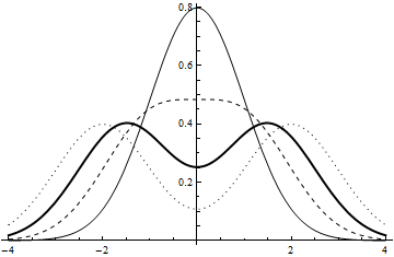
Consider the probability measure $\mu_{s}$ on $\mathbb{R}$ given as the convex combination of two gaussians with means at $s$ and $-s$, with density

$$f_{s}:=\mbox{$\frac{1}{2}$}\mathcal{N}\!(s,1)+\mbox{$\frac{1}{2}$}\mathcal{N}\!(-s,1),$$

where $s\geq 0$. Observe that with $s\to\infty$ the initial density $\mathcal{N}\!(0,1)$ separates into two almost independent gaussians.

To check for which $s$ the Gaussian divergence will see this behavior, we fix the partition $(-\infty,0),(0,\infty)$. One can easily verify that

$$\begin{array}[]{l}d_{\mu_{s}}\big{(}\mathcal{G};((-\infty,0),(0,\infty))\big{)}=\\ -\ln(2)+\frac{1}{2}\ln(1+s^{2})-\frac{1}{2}\ln[1-\frac{2e^{-s^{2}}}{\pi}+s^{2}\!-\sqrt{\frac{8}{\pi}}se^{-\frac{s^{2}}{2}}\mathrm{Erf}(\frac{s}{\sqrt{2}})-s^{2}\mathrm{Erf}(\frac{s}{\sqrt{2}})^{2}].\end{array}$$

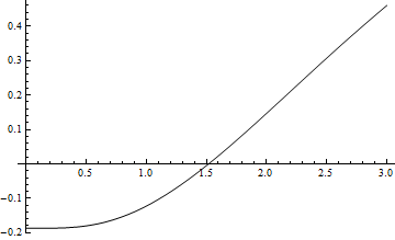
Consequently, see Figure 4(a), there exists $s_{0}\approx 1.518$ such that the clustering of $\mathbb{R}$ into two clusters $((-\infty,0),(0,\infty))$ is profitable iff $s>s_{0}$. On figure 4(b) we show densities $f_{s}$ for $s=0$ (thin line); $s=1$ (dashed line); $s=s_{0}$ (thick line) and $s=2$ (points).

This theoretical result which puts the border between one and two clusters at $s_{0}$ seems consistent with our geometrical intuition of clustering of $\mu_{s}$.

4.3 Spherical Clustering

In this section we consider spherical clustering which can be seen as a simpler version of the Gaussian clustering. By Observation 4.1 we obtain that Spherical clustering is invariant with respect to scaling and isometric transformations (however, it is obviously not invariant with respect to affine transformations).

Observation 4.3.

Let $(U_{i})_{i=1}^{k}$ be a $\mu$-partition. Then

$$\begin{array}[]{l}h_{\mu}(\mathcal{G}_{(\cdot\mathrm{I})};(U_{i})_{i=1}^{k})=\sum\limits_{i=1}^{k}\mu(U_{i})\!\cdot\![\frac{N}{2}\ln(2\pi e/N)-\ln(\mu(U_{i}))+\frac{N}{2}\ln D_{U_{i}}^{\mu}].\end{array}$$ (4.4)

To implement Hartigan approach to Spherical CEC and to deal with Spherical divergence the following trivial consequence of Theorem 3.3 is useful.

Corollary 4.1.

Let $U,V$ be measurable sets.

a) Assume additionally that $U\cap V=\emptyset$ and $\mu(U)>0,\mu(V)>0$. Then

$$\begin{array}[]{rcl}\mathrm{m}^{\mu}_{U\cup V}&=&p_{U}\mathrm{m}^{\mu}_{U}+p_{V}\mathrm{m}^{\mu}_{V},\\[4.30554pt] D^{\mu}_{U\cup V}&=&p_{U}D^{\mu}_{U}+p_{V}D^{\mu}_{V}+p_{U}p_{V}\|\mathrm{m}^{\mu}_{U}-\mathrm{m}^{\mu}_{V}\|^{2},\end{array}$$

where $p_{U}:=\frac{\mu(U)}{\mu(U)+\mu(V)},\,p_{V}:=\frac{\mu(V)}{\mu(U)+\mu(V)}$.

b) Assume that $V\subset U$ is such that $\mu(V)<\mu(U)$. Then

$$\begin{array}[]{rcl}\mathrm{m}^{\mu}_{U\setminus V}&=&q_{U}\mathrm{m}^{\mu}_{U}-q_{V}\mathrm{m}^{\mu}_{V},\\[4.30554pt] D_{U\setminus V}&=&q_{U}D^{\mu}_{U}-q_{V}D^{\mu}_{V}-q_{U}q_{V}\|\mathrm{m}^{\mu}_{U}-\mathrm{m}^{\mu}_{V}\|^{2},\end{array}$$

where $q_{U}:=\frac{\mu(U)}{\mu(U)-\mu(V)},\,q_{V}:=\frac{\mu(V)}{\mu(U)-\mu(V)}$.

Example 4.2.

(a) Three circles.

(b) k-means with $k=3$.

(c) Spherical CEC.

Figure 5: Comparison of classical k-means clustering (with $k=3$ clusters) with Spherical CEC (with initially $10$ clusters) of three ,,mouse-like” circles.

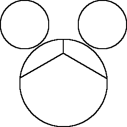
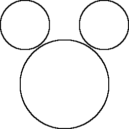
We considered the uniform distribution on the set consisting of three disjoint circlesWe started CEC with initial choice of 10 clusters, as a result of Spherical CEC we obtained clustering into three circles see Figure 5(c) – compare this result with the classical k-means with $k=3$ on Figure 5(b). Observe that contrary to classical k-means in spherical clustering we do not obtain the “mouse effect”.

Let us now consider when we should join two groups.

Theorem 4.2.

Let $U_{1}$ and $U_{2}$ be disjoint measurable sets with nonzero $\mu$-measure. We put $p_{i}=\mu(U_{i})/(\mu(U_{1})+\mu(U_{2}))$ and $\mathrm{m}_{i}=\mathrm{m}^{\mu}_{U_{i}}$, $D_{i}=D^{\mu}_{U_{i}}$ for $i=1,2$. Then

$$\begin{array}[]{l}d_{\mu}(\mathcal{G};(U_{1},U_{2}))/(\mu(U_{1})+\mu(U_{2}))\\[2.15277pt] =\frac{N}{2}\ln(p_{1}D_{1}+p_{2}D_{2}+p_{1}p_{2}\|\mathrm{m}_{1}-\mathrm{m}_{2}\|^{2})-p_{1}\frac{N}{2}\ln D_{1}-p_{2}\frac{N}{2}\ln D_{2}-\mathrm{sh}(p_{1})-\mathrm{sh}(p_{2}).\end{array}$$

Consequently, $d_{\mu}(\mathcal{G}_{(\cdot\mathrm{I})};(U_{1},U_{2}))>0$ iff

$$\|\mathrm{m}_{1}-\mathrm{m}_{2}\|^{2}>\frac{D_{1}^{p_{1}}D_{2}^{p_{2}}}{p_{1}^{2p_{1}/N}p_{2}^{2p_{2}/N}}-(p_{1}D_{1}+p_{2}D_{2}).$$

Proof.

By (4.4)

$$\begin{array}[]{l}d_{\mu}(\mathcal{G}_{(\cdot\mathrm{I})};(U_{1},U_{2}))/(\mu(U_{1})+\mu(U_{2}))\\[4.30554pt] =\frac{N}{2}\ln(D^{\mu}_{U_{1}\cup U_{2}})-p_{1}\frac{N}{2}\ln D_{1}-p_{2}\frac{N}{2}\ln D_{2}-\mathrm{sh}(p_{1})-\mathrm{sh}(p_{2}).\end{array}$$

Since by Corollary 4.1

$$D^{\mu}_{U_{1}+U_{2}}=p_{1}D_{1}+p_{2}D_{2}+p_{1}p_{2}\|\mathrm{m}_{1}-\mathrm{m}_{2}\|^{2},$$

we obtain that $d_{\mu}(\mathcal{G}_{(\cdot\mathrm{I})};(U_{1},U_{2}))>0$ iff

$$\|\mathrm{m}_{1}-\mathrm{m}_{2}\|^{2}>\frac{D_{1}^{p_{1}}D_{2}^{p_{2}}}{p_{1}^{2p_{1}/N}p_{2}^{2p_{2}/N}}-(p_{1}D_{1}+p_{2}D_{2}).$$

∎

Observation 4.4.

Let us simplify the above formula in the case when we have sets with identical measures $\mu(U_{1})=\mu(U_{2})$ and $D:=D^{\mu}_{U_{1}}=D^{\mu}_{U_{2}}$. Then by the previous theorem we should glue the groups together if

$$\|\mathrm{m}_{1}-\mathrm{m}_{2}\|\leq\sqrt{4^{1/N}-1}\cdot r,$$

where $r=\sqrt{D}$. So, as we expected, when the distance between the groups is proportional to their “radius” the joining becomes profitable.

Another, maybe less obvious, consequence of

$$4^{1/N}-1\approx\frac{\ln 4}{N}\to 0\mbox{ as }N\to\infty$$

is that with the dimension $N$ growing we should join the groups/sets together if their centers become closer. This follows from the observation that if we choose two balls in $\mathbb{R}^{N}$ with radius $r$ and distance between centers $R\geq 2r$, the proportion of their volumes to the volume of the containing ball decreases to zero with dimension growing to infinity.

4.4 Fixed covariance

In this section we are going to discuss the simple case when we cluster by $\mathcal{G}_{\Sigma}$, for a fixed $\Sigma$. By Observation 4.1 we obtain that $\mathcal{G}_{\Sigma}$ clustering is translation invariant (however, it is obviously not invariant with respect to scaling or isometric transformations).

Observation 4.5.

Let $\Sigma$ be fixed positive symmetric matrix. and let $(U_{i})_{i=1}^{k}$ be a sequence of pairwise disjoint measurable sets. Then

$$\begin{array}[]{l}h_{\mu}(\mathcal{G}_{\Sigma};(U_{i})_{i=1}^{k})\\[4.30554pt] =\sum\limits_{i=1}^{k}\mu(U_{i})\!\cdot\!(\frac{N}{2}\ln(2\pi)+\frac{1}{2}\ln\mathrm{det}(\Sigma))+\sum\limits_{i=1}^{k}\mu(U_{i})\!\cdot\![-\ln(\mu(U_{i}))+\frac{1}{2}\mathrm{tr}(\Sigma^{-1}\Sigma^{\mu}_{U_{i}})].\end{array}$$

This implies that in the $\mathcal{G}_{\Sigma}$ clustering we search for the partition $(U_{i})_{i=1}^{k}$ which minimizes

$$\sum\limits_{i=1}^{k}\mu(U_{i})\cdot\big{[}-\ln(\mu(U_{i}))+\frac{1}{2}\mathrm{tr}(\Sigma^{-1}\Sigma^{\mu}_{U_{i}})\big{]}.$$

Now we show that in the $\mathcal{G}_{\Sigma}$ clustering, if we have two groups with centers/means sufficiently close, it always pays to “glue” the groups together into one.

Theorem 4.3.

Let $U_{1}$ and $U_{2}$ be disjoint measurable sets with nonzero $\mu$-measure. We put $p_{i}=\mu(U_{i})/(\mu(U_{1})+\mu(U_{2}))$. Then

$$\begin{array}[]{l}d_{\mu}(\mathcal{G}_{\Sigma};(U_{1},U_{2}))/(\mu(U_{1})+\mu(U_{2}))=p_{1}p_{2}\|\mathrm{m}^{\mu}_{U_{1}}-\mathrm{m}^{\mu}_{U_{2}}\|_{\Sigma}^{2}-\mathrm{sh}(p_{1})-\mathrm{sh}(p_{2}).\end{array}$$ (4.5)

Consequently $d_{\mu}(\mathcal{G}_{\Sigma};(U_{1},U_{2}))>0$ iff

$$\|\mathrm{m}^{\mu}_{U_{1}}-\mathrm{m}^{\mu}_{U_{2}}\|_{\Sigma}^{2}>\frac{\mathrm{sh}(p_{1})+\mathrm{sh}(p_{2})}{p_{1}p_{2}}.$$

Proof.

We have

$$\begin{array}[]{l}d_{\mu}(\mathcal{G}_{\Sigma};(U_{1},U_{2}))/(\mu(U_{1})+\mu(U_{2}))\\[4.30554pt] =\frac{1}{2}\mathrm{tr}(\Sigma^{-1}\Sigma^{\mu}_{U_{1}\cup U_{2}})-\frac{p_{1}}{2}\mathrm{tr}(\Sigma^{-1}\Sigma^{\mu}_{U_{1}})-\frac{p_{2}}{2}\mathrm{tr}(\Sigma^{-1}\Sigma^{\mu}_{U_{2}})-\mathrm{sh}(p_{1})-\mathrm{sh}(p_{2}).\end{array}$$ (4.6)

Let $\mathrm{m}=\mathrm{m}^{\mu}_{U_{1}}-\mathrm{m}^{\mu}_{U_{2}}$. Since $\Sigma^{\mu}_{U_{1}\cup U_{2}}=p_{1}\Sigma^{\mu}_{U_{1}}+p_{2}\Sigma^{\mu}_{U_{2}}+p_{1}p_{2}\mathrm{m}\mathrm{m}^{T},$ and $\mathrm{tr}(AB)=\mathrm{tr}(BA)$, (4.6) simplifies to (4.5). ∎

Observe that the above formula is independent of deviations in groups, but only on the distance of the centers of weights (means in each groups).

Lemma 4.1.

The function

$$\{(p_{1},p_{2})\in(0,1)^{2}:p_{1}+p_{2}=1\}\to\frac{\mathrm{sh}(p_{1})+\mathrm{sh}(p_{2})}{p_{1}p_{2}}$$

attains global minimum $\ln 16$ at $p_{1}=p_{2}=1/2$.

Proof.

Consider

$$w:(0,1)\ni p\to\frac{\mathrm{sh}(p)+\mathrm{sh}(1-p)}{p(1-p)}.$$

Since $w$ is symmetric with respect to $1/2$, to show assertion it is sufficient to prove that $w$ is convex.

We have

$$\!w^{\prime\prime}(p)\!=\!\frac{2(-1\!+\!p)^{3}\ln(1\!-\!p)+p\left(-1\!+\!p\!-\!2p^{2}\ln(p)\right)}{(1\!-\!p)^{3}p^{3}}.$$

Since the denominator of $w^{\prime\prime}$ is nonnegative, we consider only the numerator, which we denote by $g(p)$. The fourth derivative of $g$ equals $12/[p(1-p)]$. This implies that

$$g^{\prime\prime}(p)=4(-2+3(-1+p)\ln(1-p)-3p\ln(p))$$

is convex, and since it is symmetric around $1/2$, it has the global minimum at $1/2$ which equals

$$g^{\prime\prime}(1/2)=4(-2+3\ln 2)=4\ln(8/e^{2})>0.$$

Consequently $g^{\prime\prime}(p)>0$ for $p\in(0,1)$, which implies that $g$ is convex. Being symmetric around $1/2$ it attains minimum at $1/2$ which equals $g(1/2)=\frac{1}{4}\ln(4/e)>0,$ which implies that $g$ is nonnegative, and consequently $w^{\prime\prime}$ is also nonegative. Therefore $w$ is convex and symmetric around $1/2$, and therefore attains its global minimum $4\ln 2$ at $p=1/2$. ∎

Corollary 4.2.

If we have two clusters with centers $\mathrm{m}_{1}$ and $\mathrm{m}_{2}$, then it is always profitable to glue them together into one group in $\mathcal{G}_{\Sigma}$-clustering if

$$\|m_{1}-m_{2}\|_{\Sigma}<\sqrt{\ln 16}\approx 1.665.$$

As a direct consequence we get:

Corollary 4.3.

Let $\mu$ be a measure with support contained in a bounded convex set $V$. Then the number of clusters which realize the cross-entropy $\mathcal{G}_{\Sigma}$ is bounded from above by the maximal cardinality of an $\varepsilon$-net (with respect to the Mahalanobis distance $\|\cdot\|_{\Sigma}$), where $\varepsilon=\sqrt{4\ln 2}$, in $V$.

Proof.

By $k$ we denote the maximal cardinality of the $\varepsilon$-net with respect to the Mahalanobis distance.

Consider an arbitrary $\mu$-partition $(U_{i})_{i=1}^{l}$ consisting of sets with nonempty $\mu$-measure. Suppose that $l>k$. We are going to construct a $\mu$-partition with $l-1$ elements which has smaller cross-entropy then $(U_{i})$.

To do so consider the set $(\mathrm{m}^{\mu}_{U_{i}})_{i=1}^{l}$ consisting of centers of the sets $U_{i}$. By the assumptions we know that there exist at least two centers which are closer then $\varepsilon$ – for simplicity assume that $\|\mathrm{m}^{\mu}_{U_{l-1}}-\mathrm{m}^{\mu}_{U_{l}}\|_{\Sigma}<\varepsilon$. Then by the previous results we obtain that

$$h_{\mu}(\mathcal{G}_{\Sigma};U_{l-1}\cup U_{l})<h_{\mu}(\mathcal{G}_{\Sigma};U_{l-1})+h_{\mu}(\mathcal{G}_{\Sigma};U_{l}).$$

This implies that the $\mu$-partition $(U_{1},\ldots,U_{l-2},U_{l-1}\cup U_{l})$ has smaller cross-entropy then $(U_{i})_{i=1}^{l}$. ∎

4.5 Spherical CEC with scale and $k$-means

We recall that $\mathcal{G}_{s\mathrm{I}}$ denotes the set of all normal densities with covariance $s\mathrm{I}$. We are going to show that for $s\to 0$ results of $\mathcal{G}_{s\mathrm{I}}$-CEC converge to k-means clustering, while for $s\to\infty$ our data will form one big group.

Observation 4.6.

For the sequence $(U_{i})_{i=1}^{k}$ we get

$$\begin{array}[]{l}h_{\mu}(\mathcal{G}_{s\mathrm{I}};(U_{i})_{i=1}^{k})=\sum\limits_{i=1}^{k}\mu(U_{i})\cdot(\frac{N}{2}\ln(2\pi s)-\ln\mu(U_{i})+\frac{N}{2s}D^{\mu}_{U_{i}}).\end{array}$$

Clearly by Observation 4.1 $\mathcal{G}_{s\mathrm{I}}$ clustering is isometry invariant, however it is not scale invariant.

To compare k-means with Spherical CEC with fixed scale let us first describe classical k-means from our point of view. Let $\mu$ denote the discrete or continuous probability measure. For a $\mu$-partition $(U_{i})_{i=1}^{k}$ we introduce the within clusters sum of squares by the formula

$$\begin{array}[]{l}\mathbf{ss}(\mu\|(U_{i})_{i=1}^{k}):=\sum\limits_{i=1}^{k}\int_{U_{i}}\|x-\mathrm{m}^{\mu}_{U_{i}}\|^{2}d\mu(x)\\[4.30554pt] =\sum\limits_{i=1}^{k}\mu(U_{i})\int\!\|x-\mathrm{m}^{\mu}_{U_{i}}\|^{2}d\mu_{U_{i}}(x)=\sum\limits_{i=1}^{k}\mu(U_{i})\!\cdot\!D_{U_{i}}^{\mu}.\end{array}$$

Remark 4.3.

Observe that if we have data $\mathrm{Y}$ partitioned into $\mathrm{Y}=\mathrm{Y}_{1}\cup\ldots\cup\mathrm{Y}_{k}$, then the above coincides (modulo multiplication by the cardinality of $\mathrm{Y}$) with the classical within clusters sum of squares. Namely, for discrete probability measure $\mu_{Y}:=\frac{1}{\mathrm{card}(\mathrm{Y})}\sum\limits_{y\in\mathrm{Y}}\delta_{y}$ we have $\mathbf{ss}(\mu_{\mathrm{Y}}\|(\mathrm{Y}_{i})_{i=1}^{k})=\frac{1}{\mathrm{card}(\mathrm{Y})}\sum\limits_{i=1}^{k}\sum\limits_{y\in\mathrm{Y}_{i}}\|y-\mathrm{m}_{\mathrm{Y}_{i}}\|^{2}$.

In classical k-means the aim is to find such $\mu$-partition $(U_{i})_{i=1}^{k}$ which minimizes the within clusters sum of squares

$$\sum_{i=1}^{k}\mu(U_{i})\cdot D^{\mu}_{U_{i}},$$ (4.7)

while in $\mathcal{G}_{s\mathrm{I}}$-clustering our aim is to minimize

$$\sum_{i=1}^{k}\mu(U_{i})\cdot(-\frac{2s}{N}\ln\mu(U_{i})+D^{\mu}_{U_{i}}).$$

Obviously with $s\to 0$, the above function converges to (4.7), which implies that k-means clustering can be understood as the limiting case of $\mathcal{G}_{s\mathrm{I}}$ clustering, with $s\to 0$.

Example 4.3.

(a) k-means with $k\!=\!5$.​

(b) $\mathcal{G}_{s\mathrm{I}}$-CEC for $s\!=\!5\!\cdot 10^{-5}$ and $5$ clusters.​

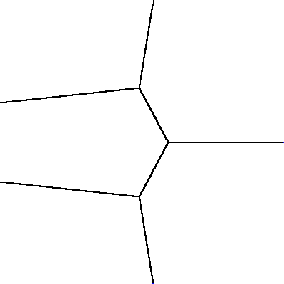
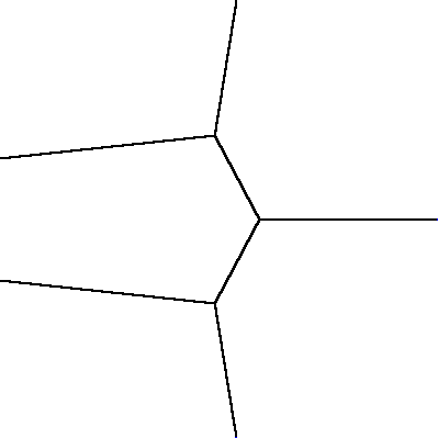
We compare on Figure 6(b) $\mathcal{G}_{s\mathrm{I}}$ clustering of the square $[0,1]^{2}$ with very small $s=5\cdot 10^{-5}$ to k-means. As we see we obtain optically identical results.

Observation 4.7.

We have

$$\begin{array}[]{l}0\leq\mathbf{ss}(\mu\|(U_{i})_{i=1}^{k})-[-s\ln(2\pi s)+\frac{2s}{N}H^{\times}\!\big{(}\mu\|\operatorname*{\uplus}\limits_{i=1}^{k}(\mathcal{G}_{s\mathrm{I}}|U_{i})\big{)}]\\ =\frac{s}{2N}\sum\limits_{i=1}^{k}\mu(U_{i})\cdot\ln(\mu(U_{i}))\leq\frac{\ln(k)}{2N}s.\end{array}$$

This means that for an arbitrary partition consisting of k-sets $\mathbf{ss}(\mu\|\cdot)$ can be approximated (as $s\to 0$) with the affine combination of $H^{\times}\!\big{(}\mu\|\mathcal{G}_{s\mathrm{I}}\big{)}$, which can be symbolically summarized as interpretation of k-means as $\mathcal{G}_{0\cdot\mathrm{I}}$ clustering.

If we cluster with $s\to\infty$ we have tendency to build larger and larger clusters.

Proposition 4.1.

Let $\mu$ be a measure with support of diameter $d$. Then for

$$s>\frac{d^{2}}{\ln 16}$$

the optimal clustering with respect to $\mathcal{G}_{s\mathrm{I}}$ will be obtained for one large group.

More precisely, for every $k>1$ and $\mu$-partition $(U_{i})_{i=1}^{k}$ consisting of sets of nonempty $\mu$-measure we have

$$H^{\times}\!\big{(}\mu\|\mathcal{F}\big{)}<H^{\times}\!\big{(}\mu\|\operatorname*{\uplus}_{i=1}^{k}(\mathcal{F}|U_{i})\big{)}.$$

Proof.

By applying Corollary 4.2 with $\Sigma=s\mathrm{I}$ we obtain that we should always glue two groups with centers $\mathrm{m}_{1},\mathrm{m}_{2}$ together if $\|\mathrm{m}_{1}-\mathrm{m}_{2}\|^{2}_{s\mathrm{I}}<\ln 16$, or equivalently if $\|\mathrm{m}_{1}-\mathrm{m}_{2}\|^{2}<s\ln 16$. ∎

Concluding, if the radius tends to zero, we cluster the data into smaller and smaller groups, while for the radius going to $\infty$, the data will have the tendency to form only one group.

References

- Hartigan [1975] J. Hartigan, Clustering algorithms, John Willey and Sons, 1975.
- Jain and Dubes [1988] A. Jain, R. Dubes, Algorithms for clustering data, Prentice-Hall, Inc., 1988.
- Jain et al. [1999] A. Jain, M. Murty, P. Flynn, Data clustering: A Review, ACM Computing Surveys 31 (1999) 264–323.
- Jain [2010] A. Jain, Data clustering: 50 years beyond K-means, Pattern Recognition Letters 31 (2010) 651–666.
- Xu and Wunsch [2009] R. Xu, D. Wunsch, Clustering, Wiley-IEEE Press, 2009.
- Bock [2007] H. Bock, Clustering methods: a history of K-Means algorithms, Selected contributions in data analysis and classification (2007) 161–172.
- Bock [2008] H. Bock, Origins and extensions of the k-means algorithm in cluster analysis, Journal Electronique d Histoire des Probabilités et de la Statistique Electronic Journal for History of Probability and Statistics 4 (2008).
- Tibshirani et al. [2001] R. Tibshirani, G. Walther, T. Hastie, Estimating the number of clusters in a data set via the gap statistic, Journal of the Royal Statistical Society: Series B (Statistical Methodology) 63 (2001) 411–423.
- Mirkin [2011] B. Mirkin, Choosing the number of clusters, Wiley Interdisciplinary Reviews: Data Mining and Knowledge Discovery 1 (2011) 252–260.
- McLachlan and Krishnan [1997] G. McLachlan, T. Krishnan, The EM algorithm and extensions, volume 274, Wiley New York, 1997.
- Samé et al. [2007] A. Samé, C. Ambroise, G. Govaert, An online classification EM algorithm based on the mixture model, Statistics and Computing 17 (2007) 209–218.
- Celeux and Govaert [1995] G. Celeux, G. Govaert, Gaussian parsimonious clustering models, Pattern Recognition 28 (1995) 781–793.
- Estivill-Castro and Yang [2000] V. Estivill-Castro, J. Yang, Fast and robust general purpose clustering algorithms, PRICAI 2000 Topics in Artificial Intelligence (2000) 208–218.
- Massa et al. [1999] S. Massa, M. Paolucci, P. Puliafito, A new modeling technique based on Markov chains to mine behavioral patterns in event based time series, DataWarehousing and Knowledge Discovery (1999) 802–802.
- Tabor and Misztal [2012] J. Tabor, K. Misztal, Detection of elliptical shapes via cross-entropy clustering, 2012. Available from http://arxiv.org/abs/1211.5712.
- Cover et al. [1991] T. Cover, J. Thomas, J. Wiley, et al., Elements of information theory, volume 6, Wiley Online Library, 1991.
- MacKay [2003] D. MacKay, Information theory, inference, and learning algorithms, Cambridge Univ Pr, 2003.
- Kullback [1997] S. Kullback, Information theory and statistics, Dover Pubns, 1997.
- Shannon [2001] C. Shannon, A mathematical theory of communication, ACM SIGMOBILE Mobile Computing and Communications Review 5 (2001) 3–55.
- Grünwald [2007] P. Grünwald, The minimum description length principle, The MIT Press, 2007.
- Grünwald et al. [2005] P. Grünwald, I. Myung, M. Pitt, Advances in minimum description length: Theory and applications, the MIT Press, 2005.
- Ma et al. [2007] Y. Ma, H. Derksen, W. Hong, J. Wright, Segmentation of multivariate mixed data via lossy data coding and compression, Pattern Analysis and Machine Intelligence, IEEE Transactions on 29 (2007) 1546–1562.
- Yang et al. [2008] A. Yang, J. Wright, Y. Ma, S. Sastry, Unsupervised segmentation of natural images via lossy data compression, Computer Vision and Image Understanding 110 (2008) 212–225.
- Fahim et al. [2008] A. Fahim, G. Saake, A. Salem, F. Torkey, M. Ramadan, K-means for spherical clusters with large variance in sizes, Journal of World Academy of Science, Engineering and Technology (2008).
- Davis-Stober et al. [2007] C. Davis-Stober, S. Broomell, F. Lorenz, Exploratory data analysis with MATLAB, Psychometrika 72 (2007) 107–108.
- De Maesschalck et al. [2000] R. De Maesschalck, D. Jouan-Rimbaud, D. Massart, The mahalanobis distance, Chemometrics and Intelligent Laboratory Systems 50 (2000) 1–18.
- Aloise et al. [2009] D. Aloise, A. Deshpande, P. Hansen, P. Popat, NP-hardness of Euclidean sum-of-squares clustering, Machine Learning 75 (2009) 245–248.
- Arthur and Vassilvitskii [2007] D. Arthur, S. Vassilvitskii, k-means++: The advantages of careful seeding, in: Proceedings of the eighteenth annual ACM-SIAM symposium on Discrete algorithms, Society for Industrial and Applied Mathematics, pp. 1027–1035.
- Shioda and Tunçel [2007] R. Shioda, L. Tunçel, Clustering via minimum volume ellipsoids, Computational Optimization and Applications 37 (2007) 247–295.