Entanglement negativity in extended systems: A field theoretical approach

Pasquale Calabrese1, John Cardy2, and Erik Tonni3 1 Dipartimento di Fisica dell’Università di Pisa and INFN, Pisa, Italy.
2 Oxford University, Rudolf Peierls Centre for Theoretical Physics, 1 Keble Road, Oxford, OX1 3NP, United Kingdom and All Souls College, Oxford.
3 SISSA and INFN, via Bonomea 265, 34136 Trieste, Italy.
Abstract

We report on a systematic approach for the calculation of the negativity in the ground state of a one-dimensional quantum field theory. The partial transpose ρAT2superscriptsubscript𝜌𝐴subscript𝑇2\rho_{A}^{T_{2}} of the reduced density matrix of a subsystem A=A1A2𝐴subscript𝐴1subscript𝐴2A=A_{1}\cup A_{2} is explicitly constructed as an imaginary-time path integral and from this the replicated traces Tr(ρAT2)nTrsuperscriptsuperscriptsubscript𝜌𝐴subscript𝑇2𝑛{\rm Tr}(\rho_{A}^{T_{2}})^{n} are obtained. The logarithmic negativity =logρAT2normsuperscriptsubscript𝜌𝐴subscript𝑇2{\cal E}=\log||\rho_{A}^{T_{2}}|| is then the continuation to n1𝑛1n\to 1 of the traces of the even powers. For pure states, this procedure reproduces the known results. We then apply this method to conformally invariant field theories in several different physical situations for infinite and finite systems and without or with boundaries. In particular, in the case of two adjacent intervals of lengths 1,2subscript1subscript2\ell_{1},\ell_{2} in an infinite system, we derive the result (c/4)ln(12/(1+2))similar-to𝑐4subscript1subscript2subscript1subscript2{\cal E}\sim(c/4)\ln(\ell_{1}\ell_{2}/(\ell_{1}+\ell_{2})), where c𝑐c is the central charge. For the more complicated case of two disjoint intervals, we show that the negativity depends only on the harmonic ratio of the four end-points and so is manifestly scale invariant. We explicitly calculate the scale-invariant functions for the replicated traces in the case of the CFT for the free compactified boson, but we have not so far been able to obtain the n1𝑛1n\to 1 continuation for the negativity even in the limit of large compactification radius. We have checked all our findings against exact numerical results for the harmonic chain which is described by a non-compactified free boson.

Contents

\@starttoc

toc

1 Introduction

The study of the entanglement content of many-body quantum systems has allowed in recent years a deeper understanding of these systems, in particular in connection with criticality and topological order (see [1] for reviews). In the case when a system is in its ground-state (or any given pure state) the entanglement between two complementary parts is measured by the entanglement entropies defined as follows. Let ρ𝜌\rho be the density matrix of a system, which we take to be in a pure quantum state |ΨketΨ|\Psi\rangle, so that ρ=|ΨΨ|𝜌ketΨbraΨ\rho=|\Psi\rangle\langle\Psi|. Let the Hilbert space be written as a direct product =ABtensor-productsubscript𝐴subscript𝐵\mathcal{H}=\mathcal{H}_{A}\otimes\mathcal{H}_{B}. A𝐴A’s reduced density matrix is ρA=TrBρsubscript𝜌𝐴subscriptTr𝐵𝜌\rho_{A}={\rm Tr}_{B}\rho. The entanglement entropy is the corresponding von Neumann entropy

SA=TrρAlnρA,subscript𝑆𝐴Trsubscript𝜌𝐴subscript𝜌𝐴S_{A}=-{\rm Tr}\,\rho_{A}\ln\rho_{A}\,, (1)

and analogously for SBsubscript𝑆𝐵S_{B}. When ρ𝜌\rho corresponds to a pure quantum state SA=SBsubscript𝑆𝐴subscript𝑆𝐵S_{A}=S_{B}. Other standard measures of bipartite entanglement in pure states are the Rényi entropies

SA(n)=11nlnTrρAn,subscriptsuperscript𝑆𝑛𝐴11𝑛Trsuperscriptsubscript𝜌𝐴𝑛S^{(n)}_{A}=\frac{1}{1-n}\ln{\rm Tr}\,\rho_{A}^{n}\,, (2)

that also satisfy SA(n)=SB(n)superscriptsubscript𝑆𝐴𝑛superscriptsubscript𝑆𝐵𝑛S_{A}^{(n)}=S_{B}^{(n)} whenever ρ𝜌\rho corresponds to a pure quantum state. From these definitions SA=limn1SA(n)subscript𝑆𝐴subscript𝑛1superscriptsubscript𝑆𝐴𝑛\displaystyle S_{A}=\lim_{n\to 1}S_{A}^{(n)}. All SA(n)subscriptsuperscript𝑆𝑛𝐴S^{(n)}_{A} for any n𝑛n and for pure states are entanglement monotones [2], i.e. are quantities which do not increase under LOCC (local operation and classical communication), which is a key property of any quantity to be a good measure of entanglement. The knowledge of the Rényi entropies for any n𝑛n determines also the full spectrum of the reduced density matrix [3].

For a mixed state the entanglement entropies are not longer good measures of entanglement since they mix quantum and classical correlations (e.g. in an high temperature mixed state, SAsubscript𝑆𝐴S_{A} gives the extensive result for the thermal entropy that has nothing to do with entanglement). This is also evident from the fact that SAsubscript𝑆𝐴S_{A} is no longer equal to SBsubscript𝑆𝐵S_{B}. A quantity that is easily constructed from SA(n)superscriptsubscript𝑆𝐴𝑛S_{A}^{(n)} and SB(n)superscriptsubscript𝑆𝐵𝑛S_{B}^{(n)} is the (Rényi) mutual information, defined as

IA:B(n)=SA(n)+SB(n)SAB(n),subscriptsuperscript𝐼𝑛:𝐴𝐵subscriptsuperscript𝑆𝑛𝐴subscriptsuperscript𝑆𝑛𝐵subscriptsuperscript𝑆𝑛𝐴𝐵I^{(n)}_{A:B}=S^{(n)}_{A}+S^{(n)}_{B}-S^{(n)}_{A\cup B}\,, (3)

that by definition is symmetric in A𝐴A and B𝐵B. However, IA:B(n)subscriptsuperscript𝐼𝑛:𝐴𝐵I^{(n)}_{A:B} has not all the correct properties to be an entanglement measure and indeed it is not an entanglement monotone for any n𝑛n (for example it has been shown that for most of separable mixed states it is non-zero [4]).

This has also importance for a system in a pure state, but if one is interested into the entanglement between two non-complementary parts A1subscript𝐴1A_{1} and A2subscript𝐴2A_{2}. Indeed, generically the union A1A2subscript𝐴1subscript𝐴2A_{1}\cup A_{2} is in a mixed state with density matrix ρA1A2=TrBρsubscript𝜌subscript𝐴1subscript𝐴2subscriptTr𝐵𝜌\rho_{A_{1}\cup A_{2}}={\rm Tr}_{B}\rho with B𝐵B the complement of A1A2subscript𝐴1subscript𝐴2A_{1}\cup A_{2}. As a matter of fact, also the converse is true: any mixed state can be obtained by tracing out some degrees of freedom from a properly defined larger system, a procedure called purification (see e.g. [5]).

A proper definition of the bipartite entanglement for a general mixed state (or equivalently the tripartite entanglement in a pure state) has been longly a problem because most of the proposed measures rely on algorithms rather than explicit expressions and are therefore hard to evaluate analytically (see e.g. Refs. [1, 4, 6, 7]). However a computable measurement of entanglement, called negativity, has been introduced in a seminal work by Vidal and Werner [8]. They also showed how the negativity provides bounds on a few operationally well-defined measures of entanglement (such as distillable entanglement or teleportation fidelity). The precise meaning of the negativity in quantum information has been indeed established in Ref. [8], but the main reason for its success is a practical one: the negativity is obtained from any mixed state by computing a partial transposition and then diagonalizing a matrix, while we still do not know generically how to compute any other mixed-state entanglement measures.

Following Ref. [8], the negativity is defined as follows. Let us consider a density matrix ρ𝜌\rho corresponding to a given mixed or pure state acting on a Hilbert space \mathcal{H}. Let us consider the bipartition =12tensor-productsubscript1subscript2\mathcal{H}={\cal H}_{1}\otimes{\cal H}_{2} and let us denote by |ei(1)ketsuperscriptsubscript𝑒𝑖1|e_{i}^{(1)}\rangle and |ej(2)ketsuperscriptsubscript𝑒𝑗2|e_{j}^{(2)}\rangle two arbitrary bases in the Hilbert spaces of each part. The partial transpose (e.g. with respect to the second space) of ρ𝜌\rho is defined as

ei(1)ej(2)|ρT2|ek(1)el(2)=ei(1)el(2)|ρ|ek(1)ej(2),quantum-operator-productsuperscriptsubscript𝑒𝑖1superscriptsubscript𝑒𝑗2superscript𝜌subscript𝑇2superscriptsubscript𝑒𝑘1superscriptsubscript𝑒𝑙2quantum-operator-productsuperscriptsubscript𝑒𝑖1superscriptsubscript𝑒𝑙2𝜌subscriptsuperscript𝑒1𝑘subscriptsuperscript𝑒2𝑗\langle e_{i}^{(1)}e_{j}^{(2)}|\rho^{T_{2}}|e_{k}^{(1)}e_{l}^{(2)}\rangle=\langle e_{i}^{(1)}e_{l}^{(2)}|\rho|e^{(1)}_{k}e^{(2)}_{j}\rangle, (4)

and then the logarithmic negativity as

lnρT2=lnTr|ρT2|,normsuperscript𝜌subscript𝑇2Trsuperscript𝜌subscript𝑇2{\cal E}\equiv\ln||\rho^{T_{2}}||=\ln{\rm Tr}|\rho^{T_{2}}|\,, (5)

where the trace norm ρT2normsuperscript𝜌subscript𝑇2||\rho^{T_{2}}|| is the sum of the absolute values of the eigenvalues λisubscript𝜆𝑖\lambda_{i} of ρT2superscript𝜌subscript𝑇2\rho^{T_{2}}. In Ref. [8] another measure, termed simply negativity, has been also introduced

𝒩ρT212,𝒩normsuperscript𝜌subscript𝑇212{\cal N}\equiv\frac{||\rho^{T_{2}}||-1}{2}\,, (6)

which is trivially related to {\cal E} as 𝒩=(e1)/2𝒩superscript𝑒12{\cal N}=(e^{\cal E}-1)/2. However, {\cal E} is additive, while 𝒩𝒩{\cal N} is not and for this reason we will concentrate in the following on {\cal E} from which 𝒩𝒩{\cal N} can be trivially derived. When the two parts are two microscopic degrees of freedom (e.g. spins), the negativity is equivalent to other commonly used entanglement estimators such as the concurrence [1, 9]. However the definition of the negativity is more appealing because it is basis independent and so calculable by quantum field theory (QFT) which naturally unveils universal features, in particular close to a quantum critical point. For 1D critical theories, that at low energy are also Lorentz invariant, the powerful tools of conformal field theory (CFT) can be applied.

The fact that the negativity is computable made it a remarkable tool to study the tripartite entanglement content of many body quantum systems both in their ground-state [10, 11, 12, 13, 14, 15] or out of equilibrium [16, 17]. Some studies for the bipartite entanglement at finite temperature have been presented as well [18, 19, 20]. However, only in a recent short communication [21], we carried out a more systematic and generic approach to negativity based on QFT (and in particular CFT). In the following we give detailed derivations of all results announced in Ref. [21] and report some other new findings.
Refer to caption
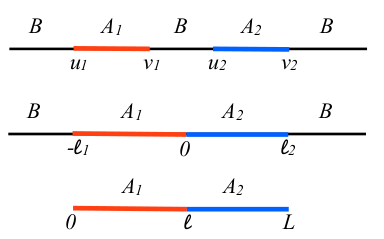
Figure 1: The three main configurations of 1D systems we consider. Top: the entanglement between two disjoint intervals A1subscript𝐴1A_{1} and A2subscript𝐴2A_{2} embedded in the ground-state of a larger system formed by the union of A1subscript𝐴1A_{1}, A2subscript𝐴2A_{2} and the remainder B𝐵B. The whole system can be either finite or infinite. Middle: The entanglement between two adjacent intervals in a larger system. Bottom: The entanglement between two adjacent intervals which form the full system (B𝐵B\to\emptyset). In all cases we denote A=A1A2𝐴subscript𝐴1subscript𝐴2A=A_{1}\cup A_{2}.

1.1 Setup and notations.

In this manuscript we only consider the entanglement, measured by the negativity, in the ground state of one-dimensional systems (1D), although some derivations have a more general validity. We focus on the tripartitions depicted in Fig. 1, i.e. the entire system is divided in three parts A1subscript𝐴1A_{1}, A2subscript𝐴2A_{2} and B𝐵B and we consider the entanglement between A1subscript𝐴1A_{1} and A2subscript𝐴2A_{2}, whose union is generically denoted with A𝐴A. As usual, A𝐴A’s reduced density matrix is ρA=TrBρsubscript𝜌𝐴subscriptTr𝐵𝜌\rho_{A}={\rm Tr}_{B}\rho. In order to lighten the notation, we will denote as ρ1subscript𝜌1\rho_{1} and ρ2subscript𝜌2\rho_{2} the reduced density matrix corresponding to A1subscript𝐴1A_{1} and A2subscript𝐴2A_{2} respectively, i.e.

ρ1subscript𝜌1\displaystyle\rho_{1} \displaystyle\equiv ρA1=TrA2(ρA)=TrBA2(ρ),subscript𝜌subscript𝐴1subscriptTrsubscript𝐴2subscript𝜌𝐴subscriptTr𝐵subscript𝐴2𝜌\displaystyle\rho_{A_{1}}={\rm Tr}_{A_{2}}(\rho_{A})={\rm Tr}_{B\cup A_{2}}(\rho)\,, (7)
ρ2subscript𝜌2\displaystyle\rho_{2} \displaystyle\equiv ρA2=TrA1(ρA)=TrBA1(ρ).subscript𝜌subscript𝐴2subscriptTrsubscript𝐴1subscript𝜌𝐴subscriptTr𝐵subscript𝐴1𝜌\displaystyle\rho_{A_{2}}={\rm Tr}_{A_{1}}(\rho_{A})={\rm Tr}_{B\cup A_{1}}(\rho)\,. (8)

Also the partial transpose with respect to A1subscript𝐴1A_{1} and A2subscript𝐴2A_{2} degrees of freedom will simply be denoted with the superscripts T1subscript𝑇1T_{1} and T2subscript𝑇2T_{2} respectively, i.e.

ρAT2ρATA2,andρAT1ρATA1.formulae-sequencesuperscriptsubscript𝜌𝐴subscript𝑇2superscriptsubscript𝜌𝐴subscript𝑇subscript𝐴2andsuperscriptsubscript𝜌𝐴subscript𝑇1superscriptsubscript𝜌𝐴subscript𝑇subscript𝐴1\rho_{A}^{T_{2}}\equiv\rho_{A}^{T_{A_{2}}}\,,\qquad{\rm and}\qquad\rho_{A}^{T_{1}}\equiv\rho_{A}^{T_{A_{1}}}\,. (9)

2 A replica approach for the negativity

2.1 Replicas and entanglement entropy.

One of the most successful approaches to calculate the entanglement entropy for a bipartite system is based on the replica trick [22] which proceeds as follows. One first calculates the traces of integer powers of the reduced density matrix

Trρ2n=iζin,Trsuperscriptsubscript𝜌2𝑛subscript𝑖superscriptsubscript𝜁𝑖𝑛{\rm Tr}\rho_{2}^{n}=\sum_{i}\zeta_{i}^{n}, (10)

where ζisubscript𝜁𝑖\zeta_{i} are the eigenvalues of the reduced density matrix ρ2subscript𝜌2\rho_{2}. Then, if one is able to analytically continue this expression to general complex n𝑛n, the entanglement entropy is given by

SA2=limn1nTrρ2n=limn111nlnTrρ2n.subscript𝑆subscript𝐴2subscript𝑛1𝑛Trsuperscriptsubscript𝜌2𝑛subscript𝑛111𝑛Trsuperscriptsubscript𝜌2𝑛S_{A_{2}}=-\lim_{n\to 1}{\partial\over\partial n}{\rm Tr}\,\rho_{2}^{n}=\lim_{n\to 1}\frac{1}{1-n}\ln{\rm Tr}\,\rho_{2}^{n}\,. (11)

It has been shown [22, 23] that, for integer n𝑛n, Trρ2nTrsuperscriptsubscript𝜌2𝑛{\rm Tr}\rho_{2}^{n} is a partition function on a complicated Riemann surface (or equivalently the correlation function of specific twist fields, as we shall review later) that is analytically achievable in a quantum field theory. The analytical properties of Trρ2nTrsuperscriptsubscript𝜌2𝑛{\rm Tr}\,\rho_{2}^{n} in the complex plane of replicas are also discussed in Refs. [24, 25].

2.2 Replicas and negativity.

A natural way to use a replica trick to compute the negativity would be to relate it to the traces of integer powers of ρT2superscript𝜌subscript𝑇2\rho^{T_{2}}. The trace norm of ρT2superscript𝜌subscript𝑇2\rho^{T_{2}} can be written in terms of its eigenvalues λisubscript𝜆𝑖\lambda_{i} as

Tr|ρT2|=i|λi|=λi>0|λi|+λi<0|λi|=1+2λi<0|λi|,Trsuperscript𝜌subscript𝑇2subscript𝑖subscript𝜆𝑖subscriptsubscript𝜆𝑖0subscript𝜆𝑖subscriptsubscript𝜆𝑖0subscript𝜆𝑖12subscriptsubscript𝜆𝑖0subscript𝜆𝑖{\rm Tr}|\rho^{T_{2}}|=\sum_{i}|\lambda_{i}|=\sum_{\lambda_{i}>0}|\lambda_{i}|+\sum_{\lambda_{i}<0}|\lambda_{i}|=1+2\sum_{\lambda_{i}<0}|\lambda_{i}|, (12)

where in the last equality we used the normalization iλi=1subscript𝑖subscript𝜆𝑖1\sum_{i}\lambda_{i}=1. This expression makes evident that the negativity measures “how much” the eigenvalues of the partial transpose of the density matrix are negative, a properties which is the reason of the name negativity.

The traces Tr(ρT2)nTrsuperscriptsuperscript𝜌subscript𝑇2𝑛{\rm Tr}(\rho^{T_{2}})^{n} of integer powers of ρT2superscript𝜌subscript𝑇2\rho^{T_{2}} have a difference dependence on |λi|subscript𝜆𝑖|\lambda_{i}| depending on the parity of n𝑛n. In the following we will always indicate an even n=2m𝑛2𝑚n=2m as nesubscript𝑛𝑒n_{e} while an odd one n=2m+1𝑛2𝑚1n=2m+1 with nosubscript𝑛𝑜n_{o}. It is understood that nesubscript𝑛𝑒n_{e} and nosubscript𝑛𝑜n_{o} refer always to the same thing, it is just the functional dependence of the traces which is different. In fact, for n𝑛n even and odd, the traces of integer powers of ρT2superscript𝜌subscript𝑇2\rho^{T_{2}} are

Tr(ρT2)neTrsuperscriptsuperscript𝜌subscript𝑇2subscript𝑛𝑒\displaystyle{\rm Tr}(\rho^{T_{2}})^{n_{e}} =\displaystyle= iλine=λi>0|λi|ne+λi<0|λi|ne,subscript𝑖superscriptsubscript𝜆𝑖subscript𝑛𝑒subscriptsubscript𝜆𝑖0superscriptsubscript𝜆𝑖subscript𝑛𝑒subscriptsubscript𝜆𝑖0superscriptsubscript𝜆𝑖subscript𝑛𝑒\displaystyle\sum_{i}\lambda_{i}^{n_{e}}=\sum_{\lambda_{i}>0}|\lambda_{i}|^{n_{e}}+\sum_{\lambda_{i}<0}|\lambda_{i}|^{n_{e}}\,, (13)
Tr(ρT2)noTrsuperscriptsuperscript𝜌subscript𝑇2subscript𝑛𝑜\displaystyle{\rm Tr}(\rho^{T_{2}})^{n_{o}} =\displaystyle= iλino=λi>0|λi|noλi<0|λi|no.subscript𝑖superscriptsubscript𝜆𝑖subscript𝑛𝑜subscriptsubscript𝜆𝑖0superscriptsubscript𝜆𝑖subscript𝑛𝑜subscriptsubscript𝜆𝑖0superscriptsubscript𝜆𝑖subscript𝑛𝑜\displaystyle\sum_{i}\lambda_{i}^{n_{o}}=\sum_{\lambda_{i}>0}|\lambda_{i}|^{n_{o}}-\sum_{\lambda_{i}<0}|\lambda_{i}|^{n_{o}}\,. (14)

If now we just set ne=1subscript𝑛𝑒1n_{e}=1 in Eq. (13) we formally obtain Tr|ρT2|Trsuperscript𝜌subscript𝑇2{\rm Tr}|\rho^{T_{2}}| in which we are interested. Oppositely, setting no=1subscript𝑛𝑜1n_{o}=1 in Eq. (14) gives the normalization TrρT2=1Trsuperscript𝜌subscript𝑇21{\rm Tr}\rho^{T_{2}}=1. This means that the analytic continuations from even and odd n𝑛n are different and the trace norm in which we are interested is obtained by considering the analytic continuation of the even sequence at ne1subscript𝑛𝑒1n_{e}\to 1, i.e.

=limne1lnTr(ρT2)ne.subscriptsubscript𝑛𝑒1Trsuperscriptsuperscript𝜌subscript𝑇2subscript𝑛𝑒{\cal E}=\lim_{n_{e}\to 1}\ln{\rm Tr}(\rho^{T_{2}})^{n_{e}}\,. (15)

We should also mention that being (ρT2)T=ρT1superscriptsuperscript𝜌subscript𝑇2𝑇superscript𝜌subscript𝑇1(\rho^{T_{2}})^{T}=\rho^{T_{1}}, it trivially holds Tr(ρT2)n=Tr(ρT1)nTrsuperscriptsuperscript𝜌subscript𝑇2𝑛Trsuperscriptsuperscript𝜌subscript𝑇1𝑛{\rm Tr}(\rho^{T_{2}})^{n}={\rm Tr}(\rho^{T_{1}})^{n} for any n𝑛n, even not integer.

At first, this approach can seem rather unnatural because what we are doing is basically propose to calculate a quantity for even numbers and at the end set this even number to 111 which is instead odd. However, similar replica calculations have been already successfully applied to other different physical problems [26, 27], showing the reasonableness of the approach.

2.3 Integer powers of the partial transpose and the negativity of a pure state.

As a first example and check of the replica trick, we consider the case of a bipartition of the Hilbert spaces =12tensor-productsubscript1subscript2{\cal H}={\cal H}_{1}\otimes{\cal H}_{2} of a pure state |ΨketΨ|\Psi\rangle with ρ=|ΨΨ|𝜌ketΨbraΨ\rho=|\Psi\rangle\langle\Psi| for which the negativity is known [8]. The Schmidt decomposition, in terms of two bases |ek(1)ketsuperscriptsubscript𝑒𝑘1|e_{k}^{(1)}\rangle and |ej(2)ketsuperscriptsubscript𝑒𝑗2|e_{j}^{(2)}\rangle in the Hilbert spaces 1subscript1{\cal H}_{1} and 2subscript2{\cal H}_{2} respectively, gives

|Ψ=jcj|ej(1)ej(2)ketΨsubscript𝑗subscript𝑐𝑗ketsubscriptsuperscript𝑒1𝑗subscriptsuperscript𝑒2𝑗|\Psi\rangle=\sum_{j}c_{j}\,|e^{(1)}_{j}e^{(2)}_{j}\rangle (16)

where the coefficient cjsubscript𝑐𝑗c_{j} can be chosen such that cj[0,1]subscript𝑐𝑗01c_{j}\in[0,1]. We also have

ρ=j,kcjck|ej(1)ej(2)ek(1)ek(2)|,ρ2=Tr1(ρ)=jck2|ek(2)ek(2)|,formulae-sequence𝜌subscript𝑗𝑘subscript𝑐𝑗subscript𝑐𝑘ketsubscriptsuperscript𝑒1𝑗subscriptsuperscript𝑒2𝑗brasubscriptsuperscript𝑒1𝑘subscriptsuperscript𝑒2𝑘subscript𝜌2subscriptTr1𝜌subscript𝑗superscriptsubscript𝑐𝑘2ketsubscriptsuperscript𝑒2𝑘brasubscriptsuperscript𝑒2𝑘\rho=\sum_{j,k}c_{j}c_{k}|e^{(1)}_{j}e^{(2)}_{j}\rangle\langle e^{(1)}_{k}e^{(2)}_{k}|\,,\qquad\rho_{2}={\rm Tr}_{1}(\rho)=\sum_{j}c_{k}^{2}|e^{(2)}_{k}\rangle\langle e^{(2)}_{k}|\,, (17)

where ρ2subscript𝜌2\rho_{2} is the reduced density matrix on 2subscript2{\cal H}_{2}.

The partial transpose of the density matrix is then

ρT2=j,kcjck|ej(1)ek(2)ek(1)ej(2)|,superscript𝜌subscript𝑇2subscript𝑗𝑘subscript𝑐𝑗subscript𝑐𝑘ketsubscriptsuperscript𝑒1𝑗subscriptsuperscript𝑒2𝑘brasubscriptsuperscript𝑒1𝑘subscriptsuperscript𝑒2𝑗\rho^{T_{2}}=\sum_{j,k}c_{j}c_{k}|e^{(1)}_{j}e^{(2)}_{k}\rangle\langle e^{(1)}_{k}e^{(2)}_{j}|\,, (18)

whose n𝑛n-th power reads

(ρT2)nsuperscriptsuperscript𝜌subscript𝑇2𝑛\displaystyle(\rho^{T_{2}})^{n} =\displaystyle= j1,,jnk1,,kncj1ck1cj2ck2cjncknsubscriptsubscript𝑗1subscript𝑗𝑛subscript𝑘1subscript𝑘𝑛subscript𝑐subscript𝑗1subscript𝑐subscript𝑘1subscript𝑐subscript𝑗2subscript𝑐subscript𝑘2subscript𝑐subscript𝑗𝑛subscript𝑐subscript𝑘𝑛\displaystyle\sum_{\tiny\begin{array}[]{c}j_{1},\dots,j_{n}\\ k_{1},\dots,k_{n}\end{array}}c_{j_{1}}c_{k_{1}}c_{j_{2}}c_{k_{2}}\dots c_{j_{n}}c_{k_{n}}
×|ek1(2)ej1(1)ej1(2)ek1(1)|ek2(2)ej2(1)ej2(2)ek2(1)||ekn(2)ejn(1)ejn(2)ekn(1)|=\displaystyle\qquad\times\,|e^{(2)}_{k_{1}}e^{(1)}_{j_{1}}\rangle\langle e^{(2)}_{j_{1}}e^{(1)}_{k_{1}}|e^{(2)}_{k_{2}}e^{(1)}_{j_{2}}\rangle\langle e^{(2)}_{j_{2}}e^{(1)}_{k_{2}}|\dots|e^{(2)}_{k_{n}}e^{(1)}_{j_{n}}\rangle\langle e^{(2)}_{j_{n}}e^{(1)}_{k_{n}}|=
=\displaystyle= j1,,jnk1,,kncj1ck1cj2ck2cjncknsubscriptsubscript𝑗1subscript𝑗𝑛subscript𝑘1subscript𝑘𝑛subscript𝑐subscript𝑗1subscript𝑐subscript𝑘1subscript𝑐subscript𝑗2subscript𝑐subscript𝑘2subscript𝑐subscript𝑗𝑛subscript𝑐subscript𝑘𝑛\displaystyle\sum_{\tiny\begin{array}[]{c}j_{1},\dots,j_{n}\\ k_{1},\dots,k_{n}\end{array}}c_{j_{1}}c_{k_{1}}c_{j_{2}}c_{k_{2}}\dots c_{j_{n}}c_{k_{n}} (25)
×|ek1(2)ej1(1)δj1,k2δk1,j2δj2,k3δk2,j3δjn1,knδkn1,jnejn(2)ekn(1)|.absentketsubscriptsuperscript𝑒2subscript𝑘1subscriptsuperscript𝑒1subscript𝑗1subscript𝛿subscript𝑗1subscript𝑘2subscript𝛿subscript𝑘1subscript𝑗2subscript𝛿subscript𝑗2subscript𝑘3subscript𝛿subscript𝑘2subscript𝑗3subscript𝛿subscript𝑗𝑛1subscript𝑘𝑛subscript𝛿subscript𝑘𝑛1subscript𝑗𝑛brasubscriptsuperscript𝑒2subscript𝑗𝑛subscriptsuperscript𝑒1subscript𝑘𝑛\displaystyle\qquad\times\,|e^{(2)}_{k_{1}}e^{(1)}_{j_{1}}\rangle\,\delta_{j_{1},k_{2}}\delta_{k_{1},j_{2}}\,\delta_{j_{2},k_{3}}\delta_{k_{2},j_{3}}\dots\delta_{j_{n-1},k_{n}}\delta_{k_{n-1},j_{n}}\langle e^{(2)}_{j_{n}}e^{(1)}_{k_{n}}|\,.

The sequence of deltas gives a result which depends on the parity of n𝑛n

(ρT2)n={j1,k1cj1nock1no|ek1(2)ej1(1)ej1(2)ek1(1)|,n=noodd,j1,k1cj1neck1ne|ek1(2)ej1(1)ek1(2)ej1(1)|,n=neeven,superscriptsuperscript𝜌subscript𝑇2𝑛casessubscriptsubscript𝑗1subscript𝑘1superscriptsubscript𝑐subscript𝑗1subscript𝑛𝑜superscriptsubscript𝑐subscript𝑘1subscript𝑛𝑜ketsubscriptsuperscript𝑒2subscript𝑘1subscriptsuperscript𝑒1subscript𝑗1brasubscriptsuperscript𝑒2subscript𝑗1subscriptsuperscript𝑒1subscript𝑘1𝑛subscript𝑛𝑜oddsubscriptsubscript𝑗1subscript𝑘1superscriptsubscript𝑐subscript𝑗1subscript𝑛𝑒superscriptsubscript𝑐subscript𝑘1subscript𝑛𝑒ketsubscriptsuperscript𝑒2subscript𝑘1subscriptsuperscript𝑒1subscript𝑗1brasubscriptsuperscript𝑒2subscript𝑘1subscriptsuperscript𝑒1subscript𝑗1𝑛subscript𝑛𝑒even(\rho^{T_{2}})^{n}=\left\{\begin{array}[]{ll}\displaystyle\sum_{j_{1},k_{1}}c_{j_{1}}^{n_{o}}c_{k_{1}}^{n_{o}}|e^{(2)}_{k_{1}}e^{(1)}_{j_{1}}\rangle\langle e^{(2)}_{j_{1}}e^{(1)}_{k_{1}}|,&\qquad n=n_{o}\;{\rm odd},\\ \displaystyle\sum_{j_{1},k_{1}}c_{j_{1}}^{n_{e}}c_{k_{1}}^{n_{e}}\,|e^{(2)}_{k_{1}}e^{(1)}_{j_{1}}\rangle\langle e^{(2)}_{k_{1}}e^{(1)}_{j_{1}}|,&\qquad n=n_{e}\;{\rm even},\end{array}\right. (26)

from which

Tr(ρT2)n={rcr2no=Trρ2no,n=noodd,[rcrne]2=(Trρ2ne/2)2,n=neeven.Trsuperscriptsuperscript𝜌subscript𝑇2𝑛casessubscript𝑟superscriptsubscript𝑐𝑟2subscript𝑛𝑜Trsuperscriptsubscript𝜌2subscript𝑛𝑜𝑛subscript𝑛𝑜oddsuperscriptdelimited-[]subscript𝑟superscriptsubscript𝑐𝑟subscript𝑛𝑒2superscriptTrsuperscriptsubscript𝜌2subscript𝑛𝑒22𝑛subscript𝑛𝑒even{\rm Tr}(\rho^{T_{2}})^{n}=\left\{\begin{array}[]{ll}\displaystyle\sum_{r}c_{r}^{2n_{o}}={\rm Tr}\rho_{2}^{n_{o}},&\hskip 17.07182ptn=n_{o}\;{\rm odd},\\ \displaystyle\bigg{[}\sum_{r}c_{r}^{n_{e}}\bigg{]}^{2}=\big{(}{\rm Tr}\,\rho_{2}^{n_{e}/2}\big{)}^{2},&\hskip 17.07182ptn=n_{e}\;{\rm even}.\end{array}\right. (27)

Notice in particular that

Tr(ρT2)2=Tr(ρT2)=1.Trsuperscriptsuperscript𝜌subscript𝑇22Trsuperscript𝜌subscript𝑇21{\rm Tr}(\rho^{T_{2}})^{2}={\rm Tr}(\rho^{T_{2}})=1\,. (28)

Taking the limit ne1subscript𝑛𝑒1n_{e}\to 1, we recover the result [8] that for a pure state the logarithmic negativity is the Rényi entropy of order 1/2121/2 (cf. Eq. (2) with n=1/2𝑛12n=1/2)

=SA2(1/2)=2lnTrρ21/2.subscriptsuperscript𝑆12subscript𝐴22Trsuperscriptsubscript𝜌212{\cal E}=S^{(1/2)}_{A_{2}}=2\ln{\rm Tr}\rho_{2}^{1/2}. (29)

Taking instead the limit no1subscript𝑛𝑜1n_{o}\to 1, we recover the normalization Tr(ρT2)=Trρ2=1Trsuperscript𝜌subscript𝑇2Trsubscript𝜌21\textrm{Tr}(\rho^{T_{2}})=\textrm{Tr}\rho_{2}=1.

3 Negativity and Quantum Field Theory

In this section we show how to compute for a generic tripartition of a 1D quantum field theory the integer traces of the partial transpose of the reduced density matrix and from these, via the replica trick, the logarithmic negativity. For concreteness we will only consider the tripartition of a 1D system depicted in Fig. 1 with A𝐴A composed of two parts A=A1A2=[u1,v1][u2,v2]𝐴subscript𝐴1subscript𝐴2subscript𝑢1subscript𝑣1subscript𝑢2subscript𝑣2A=A_{1}\cup A_{2}=[u_{1},v_{1}]\cup[u_{2},v_{2}] and B𝐵B the remainder, but most of the following ideas apply to more general cases (e.g. A1subscript𝐴1A_{1} and A2subscript𝐴2A_{2} made each of several disjoint intervals). In order to introduce the general formalism for the negativity, we first review in the next subsection the path integral approach to the entanglement entropy [22, 23] and the use of the twist fields [22, 24].

3.1 The reduced density matrix and the entanglement entropy in QFT.
Refer to caption
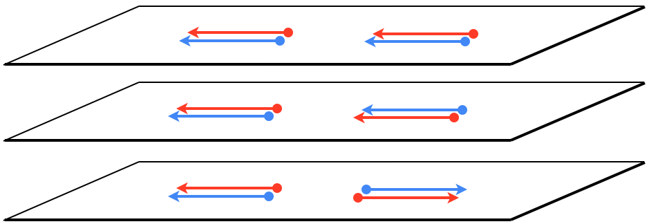
Figure 2: Top: The reduced density matrix ρAsubscript𝜌𝐴\rho_{A} o f two disjoint intervals. Middle: Partial transpose with respect to the second interval ρAT2superscriptsubscript𝜌𝐴subscript𝑇2\rho_{A}^{T_{2}}. Bottom: Reversed partial transpose ρAC2=CρAT2Csuperscriptsubscript𝜌𝐴subscript𝐶2𝐶superscriptsubscript𝜌𝐴subscript𝑇2𝐶\rho_{A}^{C_{2}}=C\rho_{A}^{T_{2}}C, where C𝐶C reverses the order of the row and column indices.

The density matrix ρ𝜌\rho in a thermal state at temperature T=1/β𝑇1𝛽T=1/\beta may be written as a path integral in the imaginary time interval (0,β)0𝛽(0,\beta)

ρ({ϕx}|{ϕx})=Z1[dϕ(y,τ)]xδ(ϕ(y,0)ϕx)xδ(ϕ(y,β)ϕx)eSE,𝜌conditionalsubscriptitalic-ϕ𝑥subscriptsuperscriptitalic-ϕsuperscript𝑥superscript𝑍1delimited-[]𝑑italic-ϕ𝑦𝜏subscriptproduct𝑥𝛿italic-ϕ𝑦0subscriptsuperscriptitalic-ϕsuperscript𝑥subscriptproduct𝑥𝛿italic-ϕ𝑦𝛽subscriptitalic-ϕ𝑥superscript𝑒subscript𝑆𝐸\rho(\{\phi_{x}\}|\{\phi^{\prime}_{x^{\prime}}\})=Z^{-1}\int[d\phi(y,\tau)]\prod_{x}\delta(\phi(y,0)-\phi^{\prime}_{x^{\prime}})\prod_{x}\delta(\phi(y,\beta)-\phi_{x})\,e^{-S_{E}}\,, (30)

where Z=TreH/T𝑍Trsuperscript𝑒𝐻𝑇Z={\rm Tr}\,e^{-H/T} is the partition function and SEsubscript𝑆𝐸S_{E} is the euclidean action. Here the rows and columns of the density matrix are labelled by the values of the fields {ϕx}subscriptitalic-ϕ𝑥\{\phi_{x}\} at τ=0,β𝜏0𝛽\tau=0,\beta. The normalization factor Z𝑍Z ensures Trρ=1Tr𝜌1{\rm Tr}\rho=1, and is found by setting {ϕx}={ϕx}subscriptitalic-ϕ𝑥subscriptsuperscriptitalic-ϕ𝑥\{\phi_{x}\}=\{\phi^{\prime}_{x}\} and integrating over these variables. In the path integral, this has the effect of sewing together the two edges to form a cylinder of circumference β𝛽\beta.

Now let us consider the subsystem A𝐴A in Fig. 1 composed of two parts A=A1A2=[u1,v1][u2,v2]𝐴subscript𝐴1subscript𝐴2subscript𝑢1subscript𝑣1subscript𝑢2subscript𝑣2A=A_{1}\cup A_{2}=[u_{1},v_{1}]\cup[u_{2},v_{2}]. The reduced density matrix ρAsubscript𝜌𝐴\rho_{A} is obtained from (30) by sewing together only those points x𝑥x which are not in A𝐴A. This has the effect of leaving two open cuts, one for each interval (uj,vj)subscript𝑢𝑗subscript𝑣𝑗(u_{j},v_{j}), along the line τ=0𝜏0\tau=0. In the limit of zero temperature, i.e. for the ground-state of the QFT, the cylinder becomes a plane as in Fig. 2 (top) where the two open cuts correspond to the rows and columns of ρAsubscript𝜌𝐴\rho_{A} and the orientation of the arrows gives the ordering of the row/column indices, e.g. increasing along the directions of the arrows.

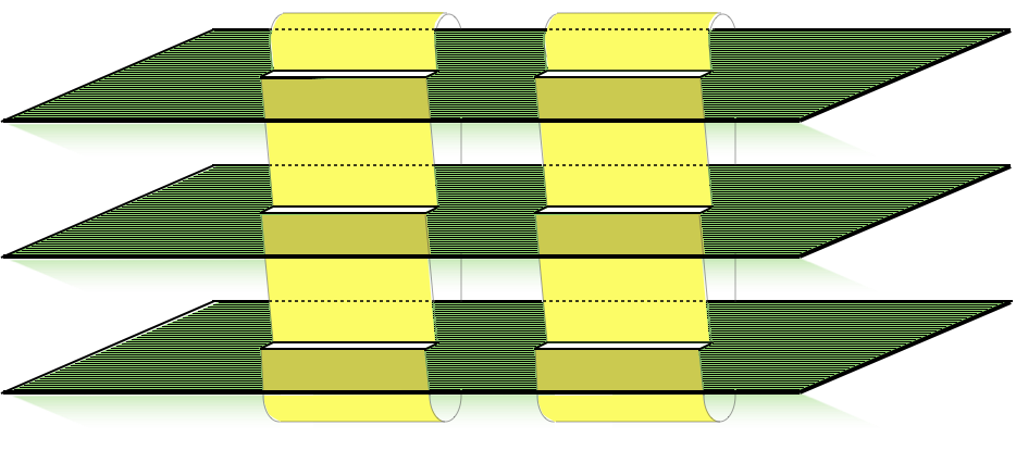
We may then compute TrρAnTrsuperscriptsubscript𝜌𝐴𝑛{\rm Tr}\,\rho_{A}^{n}, for any positive integer n𝑛n, by making n𝑛n copies of the above, labelled by an integer j𝑗j with 1jn1𝑗𝑛1\leq j\leq n, and sewing them together cyclically along the the cuts so that ϕj(x,τ=0)=ϕj+1(x,τ=0+)subscriptitalic-ϕ𝑗𝑥𝜏superscript0subscriptitalic-ϕ𝑗1𝑥𝜏superscript0\phi_{j}(x,\tau=0^{-})=\phi_{j+1}(x,\tau=0^{+}) and ϕn(x,τ=0)=ϕ1(x,τ=0+)subscriptitalic-ϕ𝑛𝑥𝜏superscript0subscriptitalic-ϕ1𝑥𝜏superscript0\phi_{n}(x,\tau=0^{-})=\phi_{1}(x,\tau=0^{+}) for all xA𝑥𝐴x\in A. This defines the n𝑛n-sheeted Riemann surface nsubscript𝑛{\cal R}_{n} depicted for n=3𝑛3n=3 in Fig. 3. Denoting with Znsubscript𝑍subscript𝑛Z_{{\cal R}_{n}} the partition function on this surface we have

TrρAn=ZnZn.Trsuperscriptsubscript𝜌𝐴𝑛subscript𝑍subscript𝑛superscript𝑍𝑛{\rm Tr}\,\rho_{A}^{n}=\frac{Z_{{\cal R}_{n}}}{Z^{n}}\,. (31)

This expression gives the Rényi entropies in Eq. (2) for integer n𝑛n and through the analytic continuation the entanglement entropy in Eq. (1).
Refer to caption
Figure 3: The path integral representation of TrρAnTrsuperscriptsubscript𝜌𝐴𝑛{\rm Tr}\rho_{A}^{n} gives a n𝑛n-sheeted Riemann surface nsubscript𝑛{\cal R}_{n} depicted here for n=3𝑛3n=3 and A=[u1,v1][u2,v2]𝐴subscript𝑢1subscript𝑣1subscript𝑢2subscript𝑣2A=[u_{1},v_{1}]\cup[u_{2},v_{2}].

As a consequence of its locality, the partition function can be expressed as an object calculated on the complex plane \mathbb{C}, where the structure of the Riemann surface is implemented through appropriate boundary conditions around the points with non-zero curvature, i.e. the partition function in a theory defined on the complex plane z=x+iτ𝑧𝑥𝑖𝜏z=x+i\tau should be written in terms of certain “fields” at z=vj𝑧subscript𝑣𝑗z=v_{j} and z=uj𝑧subscript𝑢𝑗z=u_{j}. The partition function (here [ϕ](z,z¯)delimited-[]italic-ϕ𝑧¯𝑧{\cal L}[\phi](z,{\bar{z}}) is the lagrangian density)

Zn=[dϕ]nexp[n𝑑z𝑑z¯[ϕ](z,z¯)],subscript𝑍subscript𝑛subscriptdelimited-[]𝑑italic-ϕsubscript𝑛subscriptsubscript𝑛differential-d𝑧differential-d¯𝑧delimited-[]italic-ϕ𝑧¯𝑧Z_{{\cal R}_{n}}=\int[d\phi]_{{\cal R}_{n}}\exp\left[-\int_{{\cal R}_{n}}dzd{\bar{z}}\,{\cal L}[\phi](z,{\bar{z}})\right]\,, (32)

essentially defines these fields. Following Ref. [24], it is useful to move the topology of the world-sheet (i.e. the space where the coordinates x,τ𝑥𝜏x,\tau lie) nsubscript𝑛{\cal R}_{n} to the target space (i.e. the space where the fields lie). To this aim, let us consider a model formed by n𝑛n independent copies of the original model. The partition function (32) can be re-written as the path integral on the complex plane

Zn=𝒞uj,vj[dϕ1dϕn]exp[𝑑z𝑑z¯([ϕ1](z,z¯)++[ϕn](z,z¯))],subscript𝑍subscript𝑛subscriptsubscript𝒞subscript𝑢𝑗subscript𝑣𝑗subscriptdelimited-[]𝑑subscriptitalic-ϕ1𝑑subscriptitalic-ϕ𝑛subscriptdifferential-d𝑧differential-d¯𝑧delimited-[]subscriptitalic-ϕ1𝑧¯𝑧delimited-[]subscriptitalic-ϕ𝑛𝑧¯𝑧Z_{{\cal R}_{n}}=\int_{{\cal C}_{u_{j},v_{j}}}\,[d\phi_{1}\cdots d\phi_{n}]_{\mathbb{C}}\exp\left[-\int_{\mathbb{C}}dzd{\bar{z}}\,({\cal L}[\phi_{1}](z,{\bar{z}})+\ldots+{\cal L}[\phi_{n}](z,{\bar{z}}))\right], (33)

where with 𝒞uj,vjsubscriptsubscript𝒞subscript𝑢𝑗subscript𝑣𝑗\int_{{\cal C}_{u_{j},v_{j}}} we indicated the restricted path integral with conditions

𝒞uj,vj:ϕi(x,0+)=ϕi+1(x,0),x[u1,v1][u2,v2],i=1,,n,{\cal C}_{u_{j},v_{j}}:\quad\phi_{i}(x,0^{+})=\phi_{i+1}(x,0^{-})~{},\quad x\in[u_{1},v_{1}]\cup[u_{2},v_{2}],\quad i=1,\ldots,n\,, (34)

where n+ii𝑛𝑖𝑖n+i\equiv i. The lagrangian density of the multi-copy model is

(n)[ϕ1,,ϕn](x,τ)=[ϕ1](x,τ)++[ϕn](x,τ),superscript𝑛subscriptitalic-ϕ1subscriptitalic-ϕ𝑛𝑥𝜏delimited-[]subscriptitalic-ϕ1𝑥𝜏delimited-[]subscriptitalic-ϕ𝑛𝑥𝜏{\cal L}^{(n)}[\phi_{1},\ldots,\phi_{n}](x,\tau)={\cal L}[\phi_{1}](x,\tau)+\ldots+{\cal L}[\phi_{n}](x,\tau), (35)

so that the energy density is the sum of the energy densities of the n𝑛n individual copies. Hence the expression (33) indeed defines local fields at (uj,0)subscript𝑢𝑗0(u_{j},0) and (vj,0)subscript𝑣𝑗0(v_{j},0) in the multi-copy model [24].

The local fields defined in (33) are examples of twist fields. Twist fields exist in a QFT whenever there is a global internal symmetry σ𝜎\sigma, i.e. 𝑑x𝑑τ[σϕ](x,τ)=𝑑x𝑑τ[ϕ](x,τ)differential-d𝑥differential-d𝜏delimited-[]𝜎italic-ϕ𝑥𝜏differential-d𝑥differential-d𝜏delimited-[]italic-ϕ𝑥𝜏\int dxd\tau{\cal L}[\sigma\phi](x,\tau)=\int dxd\tau{\cal L}[\phi](x,\tau). The twist fields defined by (33), called branch-point twist fields [24], are associated to the two opposite cyclic permutation symmetries ii+1maps-to𝑖𝑖1i\mapsto i+1 and i+1imaps-to𝑖1𝑖i+1\mapsto i. We can denote them simply by 𝒯nsubscript𝒯𝑛{\cal T}_{n} and 𝒯¯nsubscript¯𝒯𝑛\overline{{\cal T}}_{n}

𝒯n𝒯σ,subscript𝒯𝑛subscript𝒯𝜎\displaystyle{\cal T}_{n}\equiv{\cal T}_{\sigma}~{},\quad σ𝜎\displaystyle\sigma :ii+1modn,:absentmaps-to𝑖𝑖1mod𝑛\displaystyle\;:\;i\mapsto i+1\ {\rm mod}\,n\,, (36)
𝒯¯n𝒯σ1,subscript¯𝒯𝑛subscript𝒯superscript𝜎1\displaystyle\overline{{\cal T}}_{n}\equiv{\cal T}_{\sigma^{-1}}~{},\quad σ1superscript𝜎1\displaystyle\sigma^{-1} :i+1imodn.:absentmaps-to𝑖1𝑖mod𝑛\displaystyle\;:\;i+1\mapsto i\ {\rm mod}\,n\,. (37)

𝒯¯nsubscript¯𝒯𝑛\overline{{\cal T}}_{n} can be identified with 𝒯nsubscript𝒯𝑛{\cal T}_{-n} and 𝒯nn=𝒯¯nn=1superscriptsubscript𝒯𝑛𝑛superscriptsubscript¯𝒯𝑛𝑛1{\cal T}_{n}^{n}=\overline{{\cal T}}_{n}^{n}=1. Thus, for the n𝑛n-sheeted Riemann surface along the set A𝐴A made of the two disjoint intervals [u1,v1][u2,v2]subscript𝑢1subscript𝑣1subscript𝑢2subscript𝑣2[u_{1},v_{1}]\cup[u_{2},v_{2}], we have

TrρAn=𝒯n(u1)𝒯¯n(v1)𝒯n(u2)𝒯¯n(v2).Trsuperscriptsubscript𝜌𝐴𝑛subscriptdelimited-⟨⟩subscript𝒯𝑛subscript𝑢1subscript¯𝒯𝑛subscript𝑣1subscript𝒯𝑛subscript𝑢2subscript¯𝒯𝑛subscript𝑣2{\rm Tr}\rho_{A}^{n}=\langle{\cal T}_{n}(u_{1})\overline{\cal T}_{n}(v_{1}){\cal T}_{n}(u_{2})\overline{\cal T}_{n}(v_{2})\rangle_{\mathbb{C}}\,. (38)

In the following the subscript {\mathbb{C}} will be understood in the expectation values, if not differently stated.

3.2 The partial transposition and the negativity in QFT.
Refer to caption
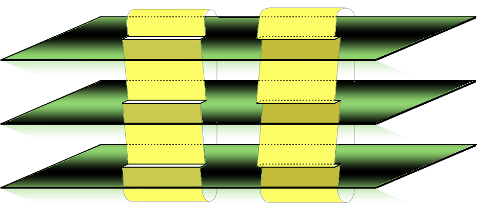
Figure 4: Path integral representation of Tr(ρAT2)n=Tr(ρAC2)nTrsuperscriptsuperscriptsubscript𝜌𝐴subscript𝑇2𝑛Trsuperscriptsuperscriptsubscript𝜌𝐴subscript𝐶2𝑛{\rm Tr}(\rho_{A}^{T_{2}})^{n}={\rm Tr}(\rho_{A}^{C_{2}})^{n} for n=3𝑛3n=3.

The partial transposition of the reduced density matrix ρAsubscript𝜌𝐴\rho_{A} with respect to the second interval A2subscript𝐴2A_{2} corresponds to the exchange of row and column indices in A2subscript𝐴2A_{2}. In the path integral representation, this is equivalent to interchange the upper and lower edges of the second cut in ρAsubscript𝜌𝐴\rho_{A} as depicted in the middle of Fig. 2. If we join n𝑛n copies of ρAT2superscriptsubscript𝜌𝐴subscript𝑇2\rho_{A}^{T_{2}} cyclically, we have an n𝑛n-sheeted Riemann surface where row and column indices are reversed compared to those of a correlation function of four twist fields, as it should be clear from the middle of Fig. 2. This problem can be however solved very easily by reversing the order of the column and row indices in A2subscript𝐴2A_{2} as in the bottom of Fig. 2, to obtain the reversed partial transpose ρAC2superscriptsubscript𝜌𝐴subscript𝐶2\rho_{A}^{C_{2}}. This is related to the partial transpose as ρAC2=CρAT2Csuperscriptsubscript𝜌𝐴subscript𝐶2𝐶superscriptsubscript𝜌𝐴subscript𝑇2𝐶\rho_{A}^{C_{2}}=C\rho_{A}^{T_{2}}C, where C𝐶C reverses the order of indices either on the lower or on the upper cut and satisfies C2=1superscript𝐶21C^{2}=1. Clearly Tr(ρAT2)n=Tr(ρAC2)nTrsuperscriptsuperscriptsubscript𝜌𝐴subscript𝑇2𝑛Trsuperscriptsuperscriptsubscript𝜌𝐴subscript𝐶2𝑛{\rm Tr}(\rho_{A}^{T_{2}})^{n}={\rm Tr}(\rho_{A}^{C_{2}})^{n} and so Tr(ρAT2)nTrsuperscriptsuperscriptsubscript𝜌𝐴subscript𝑇2𝑛{\rm Tr}(\rho_{A}^{T_{2}})^{n} is the partition function on the n𝑛n-sheeted surface obtained by joining cyclically n𝑛n of the above ρAC2superscriptsubscript𝜌𝐴subscript𝐶2\rho_{A}^{C_{2}} as in Fig. 4. In this case, the order of the row and column indices is the right one to identify this partition function with the four-point function of the twist fields

Tr(ρAT2)n=Tr(ρAC2)n=𝒯n(u1)𝒯¯n(v1)𝒯¯n(u2)𝒯n(v2),Trsuperscriptsuperscriptsubscript𝜌𝐴subscript𝑇2𝑛Trsuperscriptsuperscriptsubscript𝜌𝐴subscript𝐶2𝑛delimited-⟨⟩subscript𝒯𝑛subscript𝑢1subscript¯𝒯𝑛subscript𝑣1subscript¯𝒯𝑛subscript𝑢2subscript𝒯𝑛subscript𝑣2{\rm Tr}(\rho_{A}^{T_{2}})^{n}={\rm Tr}(\rho_{A}^{C_{2}})^{n}=\langle{\cal T}_{n}(u_{1})\overline{\cal T}_{n}(v_{1})\overline{\cal T}_{n}(u_{2}){\cal T}_{n}(v_{2})\rangle\,, (39)

i.e. the partial transposition has the net effect to exchange two twist operators compared to Eq. (38). We notice that we could easily have worked out Tr(ρAT2)nTrsuperscriptsuperscriptsubscript𝜌𝐴subscript𝑇2𝑛{\rm Tr}(\rho_{A}^{T_{2}})^{n} without introducing the reverse partial transpose. However this is a very useful technical concept because it allows to identify Tr(ρAT2)nTrsuperscriptsuperscriptsubscript𝜌𝐴subscript𝑇2𝑛{\rm Tr}(\rho_{A}^{T_{2}})^{n} with the correlation function of already known and studied twist fields, without the need of introducing new fields.

For n=2𝑛2n=2, 𝒯2=𝒯¯2subscript𝒯2subscript¯𝒯2{\cal T}_{2}=\overline{\cal T}_{2} and so

TrρA2=Tr(ρAT2)2,Trsuperscriptsubscript𝜌𝐴2Trsuperscriptsuperscriptsubscript𝜌𝐴subscript𝑇22{\rm Tr}\rho_{A}^{2}={\rm Tr}(\rho_{A}^{T_{2}})^{2}\,, (40)

which also straightforwardly follows from the properties of the trace and so it is true for any matrix ρ𝜌\rho replacing ρAsubscript𝜌𝐴\rho_{A} above.

To replace ρAT2superscriptsubscript𝜌𝐴subscript𝑇2\rho_{A}^{T_{2}} with ρAC2superscriptsubscript𝜌𝐴subscript𝐶2\rho_{A}^{C_{2}} it has been fundamental to consider integer cyclical traces. The operator C𝐶C enters in quantities like Tr(ρAρAT2)Trsubscript𝜌𝐴superscriptsubscript𝜌𝐴subscript𝑇2{\rm Tr}(\rho_{A}\rho_{A}^{T_{2}}) which is in fact the partition function on a non-orientable surface with the topology of a Klein bottle. This can also be computed using CFT methods [28].

3.3 The case of two adjacent intervals.

Eq. (39) is of general validity, but it has interesting simple and general consequences when specialized to the case of two adjacent intervals. This can be obtained by letting v1u2subscript𝑣1subscript𝑢2v_{1}\to u_{2} so that

Tr(ρAT2)n=𝒯n(u1)𝒯¯n2(u2)𝒯n(v2).Trsuperscriptsuperscriptsubscript𝜌𝐴subscript𝑇2𝑛delimited-⟨⟩subscript𝒯𝑛subscript𝑢1superscriptsubscript¯𝒯𝑛2subscript𝑢2subscript𝒯𝑛subscript𝑣2{\rm Tr}(\rho_{A}^{T_{2}})^{n}=\langle{\cal T}_{n}(u_{1})\overline{\cal T}_{n}^{2}(u_{2}){\cal T}_{n}(v_{2})\rangle\,. (41)

For arbitrary n𝑛n, this expression cannot be evaluated in general, but two cases are easily worked out.

For n=2𝑛2n=2, we have 𝒯22=1superscriptsubscript𝒯221{\cal T}_{2}^{2}=1 and so

Tr(ρAT2)2=𝒯2(u1)𝒯2(v2)=TrρA1A22.Trsuperscriptsuperscriptsubscript𝜌𝐴subscript𝑇22delimited-⟨⟩subscript𝒯2subscript𝑢1subscript𝒯2subscript𝑣2Trsuperscriptsubscript𝜌subscript𝐴1subscript𝐴22{\rm Tr}(\rho_{A}^{T_{2}})^{2}=\langle{\cal T}_{2}(u_{1}){\cal T}_{2}(v_{2})\rangle={\rm Tr}\rho_{A_{1}\cup A_{2}}^{2}\,. (42)

This relation has been derived here from QFT methods and it would be interesting to know its general validity.

For n=3𝑛3n=3, we have 𝒯¯32=𝒯3superscriptsubscript¯𝒯32subscript𝒯3\overline{\cal T}_{3}^{2}={\cal T}_{3} and so

Tr(ρAT2)3=𝒯3(u1)𝒯3(u2)𝒯3(v2).Trsuperscriptsuperscriptsubscript𝜌𝐴subscript𝑇23delimited-⟨⟩subscript𝒯3subscript𝑢1subscript𝒯3subscript𝑢2subscript𝒯3subscript𝑣2{\rm Tr}(\rho_{A}^{T_{2}})^{3}=\langle{\cal T}_{3}(u_{1}){\cal T}_{3}(u_{2}){\cal T}_{3}(v_{2})\rangle\,. (43)

3.4 The case of a single interval.

We now specialize to a pure state by letting B𝐵B\to\emptyset for which Tr(ρAT2)nTrsuperscriptsuperscriptsubscript𝜌𝐴subscript𝑇2𝑛{\rm Tr}(\rho_{A}^{T_{2}})^{n} can be worked out in full generality considering u2v1subscript𝑢2subscript𝑣1u_{2}\to v_{1} and v2u1subscript𝑣2subscript𝑢1v_{2}\to u_{1}

Tr(ρAT2)n=𝒯n2(u2)𝒯¯n2(v2).Trsuperscriptsuperscriptsubscript𝜌𝐴subscript𝑇2𝑛delimited-⟨⟩subscriptsuperscript𝒯2𝑛subscript𝑢2subscriptsuperscript¯𝒯2𝑛subscript𝑣2{\rm Tr}(\rho_{A}^{T_{2}})^{n}=\langle{\cal T}^{2}_{n}(u_{2})\overline{\cal T}^{2}_{n}(v_{2})\rangle\,. (44)

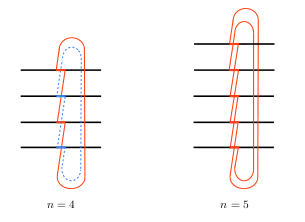
This expression depends on the parity of n𝑛n because 𝒯n2superscriptsubscript𝒯𝑛2{\cal T}_{n}^{2} connects the j𝑗j-th sheet with the (j+2)𝑗2(j+2)-th one. For n=ne𝑛subscript𝑛𝑒n=n_{e} even, the nesubscript𝑛𝑒n_{e}-sheeted Riemann surface decouples in two independent (ne/2subscript𝑛𝑒2n_{e}/2)-sheeted surfaces characterized by the parity of the sheets. Conversely for n=no𝑛subscript𝑛𝑜n=n_{o} odd, the surface remains a nosubscript𝑛𝑜n_{o}-sheeted Riemann surface (a part from a shuffling of the sheets). This is pictorially shown in Fig. 5. Thus we have

Tr(ρAT2)neTrsuperscriptsuperscriptsubscript𝜌𝐴subscript𝑇2subscript𝑛𝑒\displaystyle{\rm Tr}(\rho_{A}^{T_{2}})^{n_{e}} =\displaystyle= (𝒯ne/2(u2)𝒯¯ne/2(v2))2=(TrρA2ne/2)2,superscriptdelimited-⟨⟩subscript𝒯subscript𝑛𝑒2subscript𝑢2subscript¯𝒯subscript𝑛𝑒2subscript𝑣22superscriptTrsuperscriptsubscript𝜌subscript𝐴2subscript𝑛𝑒22\displaystyle(\langle{\cal T}_{n_{e}/2}(u_{2})\overline{\cal T}_{n_{e}/2}(v_{2})\rangle)^{2}=({\rm Tr}\rho_{A_{2}}^{n_{e}/2})^{2}\,,
Tr(ρAT2)noTrsuperscriptsuperscriptsubscript𝜌𝐴subscript𝑇2subscript𝑛𝑜\displaystyle{\rm Tr}(\rho_{A}^{T_{2}})^{n_{o}} =\displaystyle= 𝒯no(u2)𝒯¯no(v2)=TrρA2no,delimited-⟨⟩subscript𝒯subscript𝑛𝑜subscript𝑢2subscript¯𝒯subscript𝑛𝑜subscript𝑣2Trsuperscriptsubscript𝜌subscript𝐴2subscript𝑛𝑜\displaystyle\langle{\cal T}_{n_{o}}(u_{2})\overline{\cal T}_{n_{o}}(v_{2})\rangle={\rm Tr}\rho_{A_{2}}^{n_{o}}\,, (45)

which are the results for pure states in Eq. (27), recovered here purely from QFT and showing in a first simple example the effect of the parity of n𝑛n on the Riemann surfaces.

Refer to caption
Figure 5: Cut of the Riemann surface defined by 𝒯n2(u2)𝒯¯n2(v2)delimited-⟨⟩subscriptsuperscript𝒯2𝑛subscript𝑢2subscriptsuperscript¯𝒯2𝑛subscript𝑣2\langle{\cal T}^{2}_{n}(u_{2})\overline{\cal T}^{2}_{n}(v_{2})\rangle. Left: A typical example for n𝑛n even (n=4𝑛4n=4 in the figure) showing how the surface decouples in two independent parts, each with half of the sheets. Right: A typical example for n𝑛n odd (n=5𝑛5n=5 in the figure) showing that the net effect is just a reshuffling of the sheet numeration going from (1,2,3,4,5)12345(1,2,3,4,5) to (1,3,5,2,4)13524(1,3,5,2,4).

4 Negativity and conformal invariance: general results

In this section we explicitly calculate the negativity for those situations in CFT where Tr(ρAT2)nTrsuperscriptsubscriptsuperscript𝜌subscript𝑇2𝐴𝑛{\rm Tr}(\rho^{T_{2}}_{A})^{n} can be fixed by global conformal invariance and so does not depend on the operator content of the theory, but only on the central charge.

Before embarking in the full negativity calculation, we should recall that TrρAnTrsuperscriptsubscript𝜌𝐴𝑛{\rm Tr}\rho_{A}^{n}, for the case of a single interval A=[u1,v1]𝐴subscript𝑢1subscript𝑣1A=[u_{1},v_{1}], has been obtained by uniformizing the n𝑛n-sheeted Riemann surface to the complex plane [22]. This shows that the twist fields transform like primary operators of dimension [22]

Δ𝒯n=Δ𝒯¯n=c12(n1n),subscriptΔsubscript𝒯𝑛subscriptΔsubscript¯𝒯𝑛𝑐12𝑛1𝑛\Delta_{{\cal T}_{n}}={\Delta}_{\overline{\cal T}_{n}}=\frac{c}{12}\Big{(}n-\frac{1}{n}\Big{)}, (46)

where c𝑐c is the central charge. This implies (=|u1v1|subscript𝑢1subscript𝑣1\ell=|u_{1}-v_{1}|) [29, 30, 22]

TrρAn=cn(a)c/6(n1/n)SA=c3lna+c1,{\rm Tr}\rho_{A}^{n}=c_{n}\Big{(}\frac{\ell}{a}\Big{)}^{-{c}/6(n-1/n)}\quad\Rightarrow\;\;S_{A}=\frac{c}{3}\ln\frac{\ell}{a}+c^{\prime}_{1}\,, (47)

where a𝑎a is an UV cutoff (e.g. the lattice spacing) and cnsubscript𝑐𝑛c_{n} a non-universal constant, with c1=1subscript𝑐11c_{1}=1. After the normalization of the two-point function of twist fields on the plane is fixed by the constants cnsubscript𝑐𝑛c_{n}, the normalizations of two-point functions in arbitrary geometry and all other multi-point correlation functions of the twist fields are fixed and universal. Furthermore, although non-universal, the constants cnsubscript𝑐𝑛c_{n} satisfy some universal relations (see e.g. [31]).

4.1 A single interval.

Even for conformal invariant theories it is useful to specialize first to the very simple case of a reduced density matrix corresponding to a pure system, which is obtained by letting B𝐵B\to\emptyset. Thus, when A2subscript𝐴2A_{2} is embedded in an infinite system, from Eqs. (45) and (47) we have (setting =u2v2subscript𝑢2subscript𝑣2\ell=u_{2}-v_{2})

Tr(ρAT2)ne=(𝒯ne/2(u2)𝒯¯ne/2(v2))2=(TrρA2ne/2)2=cne/22(a)c/3(ne/22/ne),Trsuperscriptsuperscriptsubscript𝜌𝐴subscript𝑇2subscript𝑛𝑒superscriptdelimited-⟨⟩subscript𝒯subscript𝑛𝑒2subscript𝑢2subscript¯𝒯subscript𝑛𝑒2subscript𝑣22superscriptTrsuperscriptsubscript𝜌subscript𝐴2subscript𝑛𝑒22superscriptsubscript𝑐subscript𝑛𝑒22superscript𝑎𝑐3subscript𝑛𝑒22subscript𝑛𝑒{\rm Tr}(\rho_{A}^{T_{2}})^{n_{e}}=(\langle{\cal T}_{n_{e}/2}(u_{2})\overline{\cal T}_{n_{e}/2}(v_{2})\rangle)^{2}=({\rm Tr}\rho_{A_{2}}^{n_{e}/2})^{2}=c_{n_{e}/2}^{2}\Big{(}\frac{\ell}{a}\Big{)}^{-{c}/{3}({n_{e}}/2-2/{n_{e}})}\,, (48)

and

Tr(ρAT2)no=𝒯no(u2)𝒯¯no(v2)=TrρA2no=cno(a)c/6(no1/no).Trsuperscriptsuperscriptsubscript𝜌𝐴subscript𝑇2subscript𝑛𝑜delimited-⟨⟩subscript𝒯subscript𝑛𝑜subscript𝑢2subscript¯𝒯subscript𝑛𝑜subscript𝑣2Trsuperscriptsubscript𝜌subscript𝐴2subscript𝑛𝑜subscript𝑐subscript𝑛𝑜superscript𝑎𝑐6subscript𝑛𝑜1subscript𝑛𝑜{\rm Tr}(\rho_{A}^{T_{2}})^{n_{o}}=\langle{\cal T}_{n_{o}}(u_{2})\overline{\cal T}_{n_{o}}(v_{2})\rangle={\rm Tr}\rho_{A_{2}}^{n_{o}}=c_{n_{o}}\Big{(}\frac{\ell}{a}\Big{)}^{-{c}/6(n_{o}-1/{n_{o}})}. (49)

In spite of the simplicity of the above calculation, it shows one important point of the CFT analysis: for n=ne𝑛subscript𝑛𝑒n=n_{e} even, 𝒯ne2subscriptsuperscript𝒯2subscript𝑛𝑒{\cal T}^{2}_{n_{e}} and 𝒯¯ne2subscriptsuperscript¯𝒯2subscript𝑛𝑒\overline{\cal T}^{2}_{n_{e}} have dimensions

Δ𝒯ne2=Δ𝒯¯ne2=c6(ne22ne),subscriptΔsuperscriptsubscript𝒯subscript𝑛𝑒2subscriptΔsuperscriptsubscript¯𝒯subscript𝑛𝑒2𝑐6subscript𝑛𝑒22subscript𝑛𝑒\Delta_{{\cal T}_{n_{e}}^{2}}=\Delta_{\overline{\cal T}_{n_{e}}^{2}}=\frac{c}{6}\Big{(}\frac{n_{e}}{2}-\frac{2}{n_{e}}\Big{)}, (50)

while for n=no𝑛subscript𝑛𝑜n=n_{o} odd, 𝒯no2subscriptsuperscript𝒯2subscript𝑛𝑜{\cal T}^{2}_{n_{o}} and 𝒯¯no2subscriptsuperscript¯𝒯2subscript𝑛𝑜\overline{\cal T}^{2}_{n_{o}} have dimensions

Δ𝒯no2=Δ𝒯¯no2=c12(no1no),subscriptΔsuperscriptsubscript𝒯subscript𝑛𝑜2subscriptΔsuperscriptsubscript¯𝒯subscript𝑛𝑜2𝑐12subscript𝑛𝑜1subscript𝑛𝑜\Delta_{{\cal T}_{n_{o}}^{2}}=\Delta_{\overline{\cal T}_{n_{o}}^{2}}=\frac{c}{12}\Big{(}n_{o}-\frac{1}{n_{o}}\Big{)}, (51)

the same as 𝒯nosubscript𝒯subscript𝑛𝑜{\cal T}_{n_{o}}. Thus, performing the analytic continuation from the even branch, we finally have

||ρAT2||=limne1Tr(ρAT2)ne=c1/22(a)c/2=c2lna+2lnc1/2,||\rho_{A}^{T_{2}}||=\lim_{n_{e}\to 1}{\rm Tr}(\rho_{A}^{T_{2}})^{n_{e}}=c_{1/2}^{2}\Big{(}\frac{\ell}{a}\Big{)}^{{c}/2}\qquad\Rightarrow\;\;{\cal E}=\frac{c}{2}\ln\frac{\ell}{a}+2\ln c_{1/2}\,, (52)

which, again, just tells us that for pure states the logarithmic negativity equals the Rényi entropy of order 1/2121/2. Continuing instead to no1subscript𝑛𝑜1n_{o}\to 1 from the odd branch we obtain the normalization TrρAT2=1Trsuperscriptsubscript𝜌𝐴subscript𝑇21{\rm Tr}\rho_{A}^{T_{2}}=1.

Notice that although the various constants cno,nesubscript𝑐subscript𝑛𝑜subscript𝑛𝑒c_{n_{o},n_{e}} are non-universal, they are the same appearing in the entanglement entropies.

4.2 Two adjacent intervals.

Let us now consider the non-trivial configuration in which two intervals A1subscript𝐴1A_{1} and A2subscript𝐴2A_{2} of length 1subscript1\ell_{1} and 2subscript2\ell_{2} share a common boundary (let us say at the origin) as graphically depicted in Fig. 1. This can be obtained by letting v1u2=0subscript𝑣1subscript𝑢20v_{1}\to u_{2}=0 in Eq. (39) and it is then described by the 3-point function (we set u1=1subscript𝑢1subscript1u_{1}=-\ell_{1} and v2=2subscript𝑣2subscript2v_{2}=\ell_{2})

Tr(ρAT2)n=𝒯n(1)𝒯¯n2(0)𝒯n(2),Trsuperscriptsuperscriptsubscript𝜌𝐴subscript𝑇2𝑛delimited-⟨⟩subscript𝒯𝑛subscript1subscriptsuperscript¯𝒯2𝑛0subscript𝒯𝑛subscript2{\rm Tr}(\rho_{A}^{T_{2}})^{n}=\langle{\cal T}_{n}(-\ell_{1})\overline{\cal T}^{2}_{n}(0){\cal T}_{n}(\ell_{2})\rangle\,, (53)

whose form is determined by conformal symmetry [63]

𝒯n(1)𝒯¯n2(0)𝒯n(2)=cn2C𝒯n𝒯¯n2𝒯n(12)Δ𝒯n2(1+2)2Δ𝒯nΔ𝒯n2,delimited-⟨⟩subscript𝒯𝑛subscript1subscriptsuperscript¯𝒯2𝑛0subscript𝒯𝑛subscript2superscriptsubscript𝑐𝑛2subscript𝐶subscript𝒯𝑛subscriptsuperscript¯𝒯2𝑛subscript𝒯𝑛superscriptsubscript1subscript2subscriptΔsuperscriptsubscript𝒯𝑛2superscriptsubscript1subscript22subscriptΔsubscript𝒯𝑛subscriptΔsuperscriptsubscript𝒯𝑛2\langle{\cal T}_{n}(-\ell_{1})\overline{\cal T}^{2}_{n}(0){\cal T}_{n}(\ell_{2})\rangle=c_{n}^{2}\frac{C_{{\cal T}_{n}\overline{\cal T}^{2}_{n}{\cal T}_{n}}}{(\ell_{1}\ell_{2})^{\Delta_{{\cal T}_{n}^{2}}}(\ell_{1}+\ell_{2})^{2\Delta_{{\cal T}_{n}}-\Delta_{{\cal T}_{n}^{2}}}}, (54)

which has been normalized in such a way that the structure constant C𝒯n𝒯¯n2𝒯nsubscript𝐶subscript𝒯𝑛subscriptsuperscript¯𝒯2𝑛subscript𝒯𝑛C_{{\cal T}_{n}\overline{\cal T}^{2}_{n}{\cal T}_{n}} is universal (with all the lengths jsubscript𝑗\ell_{j} measured in units of the UV cutoff a𝑎a) and can be determined by considering the proper limit of the four-point function, as it will be done in next section.

For n=ne𝑛subscript𝑛𝑒n=n_{e} even, using the dimensions of the twist operators calculated above, we find

Tr(ρAT2)ne(12)c/6(ne/22/ne)(1+2)c/6(ne/2+1/ne),proportional-toTrsuperscriptsuperscriptsubscript𝜌𝐴subscript𝑇2subscript𝑛𝑒superscriptsubscript1subscript2𝑐6subscript𝑛𝑒22subscript𝑛𝑒superscriptsubscript1subscript2𝑐6subscript𝑛𝑒21subscript𝑛𝑒{\rm Tr}(\rho_{A}^{T_{2}})^{n_{e}}\propto{(\ell_{1}\ell_{2})^{-{c}/6({n_{e}}/2-2/{n_{e}})}(\ell_{1}+\ell_{2})^{-{c}/6({n_{e}}/2+1/{n_{e}})}}\,, (55)

that in the limit ne1subscript𝑛𝑒1n_{e}\to 1 gives

ρAT2(121+2)c/4=c4ln121+2+cnst.formulae-sequenceproportional-tonormsuperscriptsubscript𝜌𝐴subscript𝑇2superscriptsubscript1subscript2subscript1subscript2𝑐4𝑐4subscript1subscript2subscript1subscript2cnst||\rho_{A}^{T_{2}}||\propto\left(\frac{\ell_{1}\ell_{2}}{\ell_{1}+\ell_{2}}\right)^{{c}/4}\qquad\Rightarrow\quad{\cal E}=\frac{c}{4}\ln\frac{\ell_{1}\ell_{2}}{\ell_{1}+\ell_{2}}+{\rm cnst}. (56)

For n=no𝑛subscript𝑛𝑜n=n_{o} odd

Tr(ρAT2)no(12(1+2))c12(no1/no),proportional-toTrsuperscriptsuperscriptsubscript𝜌𝐴subscript𝑇2subscript𝑛𝑜superscriptsubscript1subscript2subscript1subscript2𝑐12subscript𝑛𝑜1subscript𝑛𝑜{\rm Tr}(\rho_{A}^{T_{2}})^{n_{o}}\propto(\ell_{1}\ell_{2}(\ell_{1}+\ell_{2}))^{-\frac{c}{12}(n_{o}-{1}/{n_{o}})}, (57)

that for no1subscript𝑛𝑜1n_{o}\to 1 gives again TrρAT2=1Trsuperscriptsubscript𝜌𝐴subscript𝑇21{\rm Tr}\rho_{A}^{T_{2}}=1 as it should.

Notice that for n=2𝑛2n=2, Eq. (55) is

Tr(ρAT2)2=c22C𝒯2𝒯¯22𝒯2(1+2)c/4,Trsuperscriptsuperscriptsubscript𝜌𝐴subscript𝑇22superscriptsubscript𝑐22subscript𝐶subscript𝒯2subscriptsuperscript¯𝒯22subscript𝒯2superscriptsubscript1subscript2𝑐4{\rm Tr}(\rho_{A}^{T_{2}})^{2}=c_{2}^{2}C_{{\cal T}_{2}\overline{\cal T}^{2}_{2}{\cal T}_{2}}(\ell_{1}+\ell_{2})^{-c/4}\,, (58)

which equals TrρA1A22Trsubscriptsuperscript𝜌2subscript𝐴1subscript𝐴2{\rm Tr}\rho^{2}_{A_{1}\cup A_{2}}, as predicted by Eq. (42), if C𝒯2𝒯¯22𝒯2=c21subscript𝐶subscript𝒯2subscriptsuperscript¯𝒯22subscript𝒯2superscriptsubscript𝑐21C_{{\cal T}_{2}\overline{\cal T}^{2}_{2}{\cal T}_{2}}=c_{2}^{-1}.

4.3 Finite systems.

All the previous results may be generalized to the case of a finite system of length L𝐿L with periodic boundary conditions by using a conformal mapping from the cylinder to the plane. The net effect of the mapping is to replace each length isubscript𝑖\ell_{i} with the chord length (L/π)sin(πi/L)𝐿𝜋𝜋subscript𝑖𝐿(L/\pi)\sin(\pi\ell_{i}/L) in all above formulas.

Thus for the case of a pure state in a finite system the generalization of Eqs. (48) and (49) are

Tr(ρAT2)ne=cne/22(LπasinπL)c/3(ne/22/ne),Trsuperscriptsuperscriptsubscript𝜌𝐴subscript𝑇2subscript𝑛𝑒superscriptsubscript𝑐subscript𝑛𝑒22superscript𝐿𝜋𝑎𝜋𝐿𝑐3subscript𝑛𝑒22subscript𝑛𝑒\displaystyle{\rm Tr}(\rho_{A}^{T_{2}})^{n_{e}}=c_{n_{e}/2}^{2}\Big{(}\frac{L}{\pi a}\sin\frac{\pi\ell}{L}\Big{)}^{-{c}/{3}({n_{e}}/2-2/{n_{e}})}\,, (59)
Tr(ρAT2)no=cno(LπasinπL)c/6(no1/no),Trsuperscriptsuperscriptsubscript𝜌𝐴subscript𝑇2subscript𝑛𝑜subscript𝑐subscript𝑛𝑜superscript𝐿𝜋𝑎𝜋𝐿𝑐6subscript𝑛𝑜1subscript𝑛𝑜\displaystyle{\rm Tr}(\rho_{A}^{T_{2}})^{n_{o}}=c_{n_{o}}\Big{(}\frac{L}{\pi a}\sin\frac{\pi\ell}{L}\Big{)}^{-{c}/6(n_{o}-1/{n_{o}})}\,, (60)
=c2ln(LπasinπL)+2lnc1/2.𝑐2𝐿𝜋𝑎𝜋𝐿2subscript𝑐12\displaystyle{\cal E}=\frac{c}{2}\ln\Big{(}\frac{L}{\pi a}\sin\frac{\pi\ell}{L}\Big{)}+2\ln c_{1/2}\,. (61)

For the case of two adjacent intervals the finite system generalizations of Eqs. (55) and (57) are

Tr(ρAT2)ne[L2π2sin(π1L)sin(π2L)]c/6(ne/22/ne)[Lπsinπ(1+2)L]c6(ne2+1ne),proportional-toTrsuperscriptsuperscriptsubscript𝜌𝐴subscript𝑇2subscript𝑛𝑒superscriptdelimited-[]superscript𝐿2superscript𝜋2𝜋subscript1𝐿𝜋subscript2𝐿𝑐6subscript𝑛𝑒22subscript𝑛𝑒superscriptdelimited-[]𝐿𝜋𝜋subscript1subscript2𝐿𝑐6subscript𝑛𝑒21subscript𝑛𝑒\displaystyle{\rm Tr}(\rho_{A}^{T_{2}})^{n_{e}}\propto\left[\frac{L^{2}}{\pi^{2}}\sin\Big{(}\frac{\pi\ell_{1}}{L}\Big{)}\sin\Big{(}\frac{\pi\ell_{2}}{L}\Big{)}\right]^{-{c}/6({n_{e}}/2-2/{n_{e}})}\left[\frac{L}{\pi}\sin\frac{\pi(\ell_{1}+\ell_{2})}{L}\right]^{-\frac{c}{6}(\frac{n_{e}}{2}+\frac{1}{n_{e}})}\,,
Tr(ρAT2)no[L3π3sin(π1L)sin(π2L)sinπ(1+2)L]c/12(no1/no),proportional-toTrsuperscriptsuperscriptsubscript𝜌𝐴subscript𝑇2subscript𝑛𝑜superscriptdelimited-[]superscript𝐿3superscript𝜋3𝜋subscript1𝐿𝜋subscript2𝐿𝜋subscript1subscript2𝐿𝑐12subscript𝑛𝑜1subscript𝑛𝑜\displaystyle{\rm Tr}(\rho_{A}^{T_{2}})^{n_{o}}\propto\left[\frac{L^{3}}{\pi^{3}}\sin\Big{(}\frac{\pi\ell_{1}}{L}\Big{)}\sin\Big{(}\frac{\pi\ell_{2}}{L}\Big{)}\sin\frac{\pi(\ell_{1}+\ell_{2})}{L}\right]^{-{c}/{12}(n_{o}-1/{n_{o}})}, (62)

leading to the logarithmic negativity

=c4ln[Lπsin(π1L)sin(π2L)sinπ(1+2)L]+cnst.𝑐4𝐿𝜋𝜋subscript1𝐿𝜋subscript2𝐿𝜋subscript1subscript2𝐿cnst{\cal E}=\frac{c}{4}\ln\left[\frac{L}{\pi}\frac{\sin\big{(}\frac{\pi\ell_{1}}{L}\big{)}\sin\big{(}\frac{\pi\ell_{2}}{L}\big{)}}{\sin\frac{\pi(\ell_{1}+\ell_{2})}{L}}\right]+{\rm cnst}. (63)

5 Negativity for two disjoint intervals in a CFT

For the more difficult situation of two disjoint intervals reported in Fig. 1, the entanglement entropies depend on the full operator content of the CFT and this makes much more complicated also the calculation of the negativity.

Global conformal invariance fixes the form of the four-point correlation of twist fields

𝒯n(z1)𝒯¯n(z2)𝒯n(z3)𝒯¯n(z4)=cn2|z31z42z21z43z41z32|c/6(n1/n)n(x,x¯),delimited-⟨⟩subscript𝒯𝑛subscript𝑧1subscript¯𝒯𝑛subscript𝑧2subscript𝒯𝑛subscript𝑧3subscript¯𝒯𝑛subscript𝑧4superscriptsubscript𝑐𝑛2superscriptsubscript𝑧31subscript𝑧42subscript𝑧21subscript𝑧43subscript𝑧41subscript𝑧32𝑐6𝑛1𝑛subscript𝑛𝑥¯𝑥\langle{\cal T}_{n}(z_{1})\overline{\cal T}_{n}(z_{2}){\cal T}_{n}(z_{3})\overline{\cal T}_{n}(z_{4})\rangle=c_{n}^{2}\left|\frac{z_{31}z_{42}}{z_{21}z_{43}z_{41}z_{32}}\right|^{{c}/6(n-1/n)}{\cal F}_{n}(x,\bar{x})\,, (64)

with x𝑥x the four point ratio

x=z21z43z31z42,𝑥subscript𝑧21subscript𝑧43subscript𝑧31subscript𝑧42x=\frac{z_{21}z_{43}}{z_{31}z_{42}}\,, (65)

and zij=zizjsubscript𝑧𝑖𝑗subscript𝑧𝑖subscript𝑧𝑗z_{ij}=z_{i}-z_{j}. Notice that z31z42/(z21z43z41z32)=1/(z21z43(1x))subscript𝑧31subscript𝑧42subscript𝑧21subscript𝑧43subscript𝑧41subscript𝑧321subscript𝑧21subscript𝑧431𝑥z_{31}z_{42}/(z_{21}z_{43}z_{41}z_{32})=1/(z_{21}z_{43}(1-x)). This is normalized in such a way that n(0,0)=1subscript𝑛001{\cal F}_{n}(0,0)=1 (for x0𝑥0x\to 0, the four-point function is the product of the two two-point functions normalized with cnsubscript𝑐𝑛c_{n}). The function n(x,x¯)subscript𝑛𝑥¯𝑥{\cal F}_{n}(x,\bar{x}) depends explicitly on the full operator content of the theory and must be calculated case by case. Notice that with 1(x,x¯)=1subscript1𝑥¯𝑥1{\cal F}_{1}(x,\bar{x})=1 as a consequence of TrρA=1Trsubscript𝜌𝐴1{\rm Tr}\rho_{A}=1.

Now, according to Eq. (38), TrρAnTrsuperscriptsubscript𝜌𝐴𝑛{\rm Tr}\rho_{A}^{n} corresponds in Eq. (64) to the choice

z1=u1,z2=v1z3=u2,z4=v2,formulae-sequencesubscript𝑧1subscript𝑢1formulae-sequencesubscript𝑧2subscript𝑣1formulae-sequencesubscript𝑧3subscript𝑢2subscript𝑧4subscript𝑣2z_{1}=u_{1}\,,\quad z_{2}=v_{1}\,\quad z_{3}=u_{2}\,,\quad z_{4}=v_{2}\,, (66)

and so

TrρAn=cn2((u2u1)(v2v1)(v1u1)(v2u2)(v2u1)(u2v1))c/6(n1/n)n(x),Trsuperscriptsubscript𝜌𝐴𝑛superscriptsubscript𝑐𝑛2superscriptsubscript𝑢2subscript𝑢1subscript𝑣2subscript𝑣1subscript𝑣1subscript𝑢1subscript𝑣2subscript𝑢2subscript𝑣2subscript𝑢1subscript𝑢2subscript𝑣1𝑐6𝑛1𝑛subscript𝑛𝑥{\rm Tr}\rho_{A}^{n}=c_{n}^{2}\left(\frac{(u_{2}-u_{1})(v_{2}-v_{1})}{(v_{1}-u_{1})(v_{2}-u_{2})(v_{2}-u_{1})(u_{2}-v_{1})}\right)^{{c}/6(n-1/n)}{\cal F}_{n}(x)\,, (67)

where, since for real ujsubscript𝑢𝑗u_{j} and vjsubscript𝑣𝑗v_{j} the ratio x𝑥x is real, we dropped the dependence on x¯=x¯𝑥𝑥\bar{x}=x. Explicitly, in this case x𝑥x is

x=(v1u1)(v2u2)(u2u1)(v2v1),𝑥subscript𝑣1subscript𝑢1subscript𝑣2subscript𝑢2subscript𝑢2subscript𝑢1subscript𝑣2subscript𝑣1x=\frac{(v_{1}-u_{1})(v_{2}-u_{2})}{(u_{2}-u_{1})(v_{2}-v_{1})}\,, (68)

that for the order u1<v1<u2<v2subscript𝑢1subscript𝑣1subscript𝑢2subscript𝑣2u_{1}<v_{1}<u_{2}<v_{2} satisfies 0<x<10𝑥10<x<1.

Even Tr(ρAT2)nTrsuperscriptsuperscriptsubscript𝜌𝐴subscript𝑇2𝑛{\rm Tr}(\rho_{A}^{T_{2}})^{n} is a four-point function of twist fields according to Eq. (39), but it corresponds in Eq. (64) to the choice

z1=u1,z2=v1z3=v2,z4=u2,formulae-sequencesubscript𝑧1subscript𝑢1formulae-sequencesubscript𝑧2subscript𝑣1formulae-sequencesubscript𝑧3subscript𝑣2subscript𝑧4subscript𝑢2z_{1}=u_{1}\,,\quad z_{2}=v_{1}\,\quad z_{3}=v_{2}\,,\quad z_{4}=u_{2}\,, (69)

i.e. to the exchange z3z4subscript𝑧3subscript𝑧4z_{3}\leftrightarrow z_{4} compared to TrρAnTrsuperscriptsubscript𝜌𝐴𝑛{\rm Tr}\rho_{A}^{n}. Thus we can write

Tr(ρAT2)n=cn2((v2u1)(u2v1)(v1u1)(u2v2)(u2u1)(v2v1))c/6(n1/n)n(x),Trsuperscriptsuperscriptsubscript𝜌𝐴subscript𝑇2𝑛superscriptsubscript𝑐𝑛2superscriptsubscript𝑣2subscript𝑢1subscript𝑢2subscript𝑣1subscript𝑣1subscript𝑢1subscript𝑢2subscript𝑣2subscript𝑢2subscript𝑢1subscript𝑣2subscript𝑣1𝑐6𝑛1𝑛subscript𝑛𝑥{\rm Tr}(\rho_{A}^{T_{2}})^{n}=c_{n}^{2}\left(\frac{(v_{2}-u_{1})(u_{2}-v_{1})}{(v_{1}-u_{1})(u_{2}-v_{2})(u_{2}-u_{1})(v_{2}-v_{1})}\right)^{{c}/6(n-1/n)}{\cal F}_{n}(x)\,, (70)

where x=(v1u1)(u2v2)(v2u1)(u2v1)𝑥subscript𝑣1subscript𝑢1subscript𝑢2subscript𝑣2subscript𝑣2subscript𝑢1subscript𝑢2subscript𝑣1x=\frac{(v_{1}-u_{1})(u_{2}-v_{2})}{(v_{2}-u_{1})(u_{2}-v_{1})} is again real and now satisfies <x<0𝑥0-\infty<x<0. This can be rewritten in terms of an ordered four point ratio

y=(v1u1)(v2u2)(u2u1)(v2v1)=xx1,𝑦subscript𝑣1subscript𝑢1subscript𝑣2subscript𝑢2subscript𝑢2subscript𝑢1subscript𝑣2subscript𝑣1𝑥𝑥1y=\frac{(v_{1}-u_{1})(v_{2}-u_{2})}{(u_{2}-u_{1})(v_{2}-v_{1})}=\frac{x}{x-1}\,, (71)

with 0<y<10𝑦10<y<1, as

Tr(ρAT2)n=cn2((u2u1)(v2v1)(v1u1)(v2u2)(v2u1)(u2v1))c/6(n1/n)𝒢n(y).Trsuperscriptsuperscriptsubscript𝜌𝐴subscript𝑇2𝑛superscriptsubscript𝑐𝑛2superscriptsubscript𝑢2subscript𝑢1subscript𝑣2subscript𝑣1subscript𝑣1subscript𝑢1subscript𝑣2subscript𝑢2subscript𝑣2subscript𝑢1subscript𝑢2subscript𝑣1𝑐6𝑛1𝑛subscript𝒢𝑛𝑦{\rm Tr}(\rho_{A}^{T_{2}})^{n}=c_{n}^{2}\left(\frac{(u_{2}-u_{1})(v_{2}-v_{1})}{(v_{1}-u_{1})(v_{2}-u_{2})(v_{2}-u_{1})(u_{2}-v_{1})}\right)^{{c}/6(n-1/n)}{\cal G}_{n}(y)\,. (72)

Equating equations (70) and (72), we can relate the two scaling functions n(x)subscript𝑛𝑥{\cal F}_{n}(x) and 𝒢n(y)subscript𝒢𝑛𝑦{\cal G}_{n}(y) as

𝒢n(y)=(1y)c/3(n1/n)n(yy1).subscript𝒢𝑛𝑦superscript1𝑦𝑐3𝑛1𝑛subscript𝑛𝑦𝑦1{\cal G}_{n}(y)=(1-y)^{{c}/3\left(n-{1}/n\right)}{\cal F}_{n}\Big{(}\frac{y}{y-1}\Big{)}\,. (73)

Notice that this relation does not depend on the parity of n𝑛n and so, in order to have a non-trivial replica limit ne1subscript𝑛𝑒1n_{e}\to 1 for the logarithmic negativity

(y)=limne1ln𝒢ne(y)=limne1ln[ne(yy1)],𝑦subscriptsubscript𝑛𝑒1subscript𝒢subscript𝑛𝑒𝑦subscriptsubscript𝑛𝑒1subscriptsubscript𝑛𝑒𝑦𝑦1{\cal E}(y)=\lim_{n_{e}\to 1}\ln{\cal G}_{n_{e}}(y)=\lim_{n_{e}\to 1}\ln\left[{\cal F}_{n_{e}}\Big{(}\frac{y}{y-1}\Big{)}\right]\,, (74)

some parity effect should appear in the n𝑛n dependence of the function n(x)subscript𝑛𝑥{\cal F}_{n}(x) for x<0𝑥0x<0.

The first fundamental consequence of Eq. (74) is that, for conformal invariant systems, the negativity is a scale invariant quantity (i.e. a function only of y𝑦y) because all the dimensional prefactors cancel in the replica limit. This has been argued already in the literature on the basis of numerical data [11, 12], but never proved.

It is useful to consider the ratio

Rn(y)Tr(ρAT2)nTr(ρA)n=𝒢n(y)n(y)=(1y)c/3(n1/n)n(y/(y1))n(y),subscript𝑅𝑛𝑦Trsuperscriptsuperscriptsubscript𝜌𝐴subscript𝑇2𝑛Trsuperscriptsubscript𝜌𝐴𝑛subscript𝒢𝑛𝑦subscript𝑛𝑦superscript1𝑦𝑐3𝑛1𝑛subscript𝑛𝑦𝑦1subscript𝑛𝑦R_{n}(y)\equiv\frac{{\rm Tr}(\rho_{A}^{T_{2}})^{n}}{{\rm Tr}(\rho_{A})^{n}}=\frac{{\cal G}_{n}(y)}{{\cal F}_{n}(y)}=(1-y)^{c/3(n-1/n)}\frac{{\cal F}_{n}(y/(y-1))}{{\cal F}_{n}(y)}\,, (75)

in which all the prefactors cancel. Being limn1Tr(ρA)n=1subscript𝑛1Trsuperscriptsubscript𝜌𝐴𝑛1\displaystyle\lim_{n\to 1}{\rm Tr}(\rho_{A})^{n}=1 and 1(y)=1subscript1𝑦1{\cal F}_{1}(y)=1 for 0<y<10𝑦10<y<1, we have that the negativity can be obtained just by considering replica limit of this ratio

(y)=lnlimne1Rne(y).𝑦subscriptsubscript𝑛𝑒1subscript𝑅subscript𝑛𝑒𝑦{\cal E}(y)=\ln\lim_{n_{e}\to 1}R_{n_{e}}(y)\,. (76)

The function n(x)subscript𝑛𝑥{\cal F}_{n}(x) which gives the negativity has been calculated for general integral n𝑛n only for the free compactified boson [34] and for the critical Ising model [35]. Some other partial results are also known [36, 37, 38, 39, 40, 41, 42, 43, 44, 45, 46, 47, 48, 49, 50, 51, 52]. However, the calculations in Refs. [34, 35] provide the function n(x)subscript𝑛𝑥{\cal F}_{n}(x) only for 0<x<10𝑥10<x<1 and it is a non-trivial technical problem to extend it to the domain x<0𝑥0x<0 in which we are now interested. Before embarking in these calculations, we discuss some simple and important physical consequences of Eqs. (72), (73), and (74) which are highlighted by considering the limits y1𝑦1y\to 1 and y0𝑦0y\to 0, i.e. close and far intervals respectively.

5.1 The limit of two very close intervals: y1𝑦1y\to 1.

If u2v1subscript𝑢2subscript𝑣1u_{2}\to v_{1} then y1𝑦superscript1y\to 1^{-} and we should recover the previous result for adjacent intervals. Let us denote with ϵ=u2v1italic-ϵsubscript𝑢2subscript𝑣1\epsilon=u_{2}-v_{1} and j=vjujsubscript𝑗subscript𝑣𝑗subscript𝑢𝑗\ell_{j}=v_{j}-u_{j} so that Eq. (72) becomes

Tr(ρAT2)ncn2(1(1+2)ϵ)c/6(n1/n)𝒢n(y),withy=11+212ϵ+O(ϵ2).formulae-sequencesimilar-to-or-equalsTrsuperscriptsuperscriptsubscript𝜌𝐴subscript𝑇2𝑛superscriptsubscript𝑐𝑛2superscript1subscript1subscript2italic-ϵ𝑐6𝑛1𝑛subscript𝒢𝑛𝑦with𝑦1subscript1subscript2subscript1subscript2italic-ϵ𝑂superscriptitalic-ϵ2{\rm Tr}(\rho_{A}^{T_{2}})^{n}\simeq c_{n}^{2}\left(\frac{1}{(\ell_{1}+\ell_{2})\epsilon}\right)^{c/6(n-1/n)}{\cal G}_{n}(y),\quad{\rm with}\quad y=1-\frac{\ell_{1}+\ell_{2}}{\ell_{1}\ell_{2}}\epsilon+O(\epsilon^{2})\,. (77)

This reduces to the result for adjacent intervals in Eqs. (54) only if

𝒢n(y)gn(1y)αn,similar-to-or-equalssubscript𝒢𝑛𝑦subscript𝑔𝑛superscript1𝑦subscript𝛼𝑛{\cal G}_{n}(y)\simeq g_{n}(1-y)^{\alpha_{n}}, (78)

with αnsubscript𝛼𝑛\alpha_{n} equal to Δ𝒯n2subscriptΔsuperscriptsubscript𝒯𝑛2\Delta_{{\cal T}_{n}^{2}} the dimension of 𝒯n2superscriptsubscript𝒯𝑛2{\cal T}_{n}^{2}, i.e.

αn={c6(ne22ne),ifn=neeven,c12(no1no),ifn=noodd.subscript𝛼𝑛cases𝑐6subscript𝑛𝑒22subscript𝑛𝑒if𝑛subscript𝑛𝑒evenmissing-subexpressionmissing-subexpression𝑐12subscript𝑛𝑜1subscript𝑛𝑜if𝑛subscript𝑛𝑜odd\alpha_{n}=\left\{\begin{array}[]{ll}\displaystyle\frac{c}{6}\Big{(}\frac{n_{e}}{2}-\frac{2}{n_{e}}\Big{)},&{\rm if}\;n=n_{e}\;{\rm even},\\ &\\ \displaystyle\frac{c}{12}\Big{(}n_{o}-\frac{1}{n_{o}}\Big{)},&{\rm if}\;n=n_{o}\;{\rm odd}.\end{array}\right. (79)

We stress that this power-law behavior for y𝑦y close to 111 is valid apart from possible multiplicative logarithmic corrections, whose precise form should be obtained on a case by case basis.

In the replica limit ne1subscript𝑛𝑒1n_{e}\to 1, we then have limne1αne=c/4subscriptsubscript𝑛𝑒1subscript𝛼subscript𝑛𝑒𝑐4\displaystyle\lim_{n_{e}\to 1}\alpha_{n_{e}}=-c/4, i.e. the negativity diverges approaching y=1𝑦1y=1 in the universal way

(y)=c4ln(1y).𝑦𝑐41𝑦{\cal E}(y)=-\frac{c}{4}\ln(1-y)\,. (80)

Clearly for any discrete system with a finite number of degrees of freedom in the two intervals, the negativity will remain finite in the limit of adjacent intervals, i.e. the limit of zero lattice spacing a0𝑎0a\to 0 and y1𝑦1y\to 1 do not commute (as it is well known when deriving a three-point function from the limit of the four-point one [63]). As it should be clear from the calculation above, this corresponds to set ϵ=aitalic-ϵ𝑎\epsilon=a (no distance can be smaller than the lattice spacing) and not true divergence arises in a finite discrete system. For no1subscript𝑛𝑜1n_{o}\to 1, we instead have limno1αno=0subscriptsubscript𝑛𝑜1subscript𝛼subscript𝑛𝑜0\displaystyle\lim_{n_{o}\to 1}\alpha_{n_{o}}=0 as it should to obtain the normalization TrρAT2=1Trsuperscriptsubscript𝜌𝐴subscript𝑇21{\rm Tr}\rho_{A}^{T_{2}}=1.

Furthermore the knowledge of the function 𝒢n(y)subscript𝒢𝑛𝑦{\cal G}_{n}(y) allows to calculate the universal structure constant C𝒯n𝒯¯n2𝒯nsubscript𝐶subscript𝒯𝑛superscriptsubscript¯𝒯𝑛2subscript𝒯𝑛C_{{\cal T}_{n}\overline{\cal T}_{n}^{2}{\cal T}_{n}} equating Eqs. (78) and (54), and we obtain (setting ϵ=aitalic-ϵ𝑎\epsilon=a)

C𝒯n𝒯¯n2𝒯n=gn.subscript𝐶subscript𝒯𝑛superscriptsubscript¯𝒯𝑛2subscript𝒯𝑛subscript𝑔𝑛C_{{\cal T}_{n}\overline{\cal T}_{n}^{2}{\cal T}_{n}}=g_{n}. (81)

5.2 The limit of two very far intervals: y0𝑦0y\to 0.

The limit of far intervals y0𝑦0y\to 0 can be worked out from the small x𝑥x expansion of n(x)subscript𝑛𝑥{\cal F}_{n}(x) carried out in full generality in Ref. [35]. This follows from a generalization of operator product expansion (termed short length expansion in [35]) that for the case of the entanglement entropies of two intervals give

TrρAn=cn2(12)c/6(n1/n){kj}(12n2r2)j(Δkj+Δ¯kj)s{kj}(n),Trsuperscriptsubscript𝜌𝐴𝑛superscriptsubscript𝑐𝑛2superscriptsubscript1subscript2𝑐6𝑛1𝑛subscriptsubscript𝑘𝑗superscriptsubscript1subscript2superscript𝑛2superscript𝑟2subscript𝑗subscriptΔsubscript𝑘𝑗subscript¯Δsubscript𝑘𝑗subscript𝑠subscript𝑘𝑗𝑛{\rm Tr}\,\rho_{A}^{n}=\frac{c_{n}^{2}}{(\ell_{1}\ell_{2})^{c/6(n-1/n)}}\sum_{\{k_{j}\}}\left(\frac{\ell_{1}\ell_{2}}{n^{2}r^{2}}\right)^{\sum_{j}(\Delta_{k_{j}}+{\overline{\Delta}}_{k_{j}})}s_{\{k_{j}\}}(n)\,, (82)

where the sum is over all the sets of possible operators {ϕkj}subscriptitalic-ϕsubscript𝑘𝑗\{\phi_{k_{j}}\} of the CFT with conformal dimensions (Δkj,Δ¯kjsubscriptΔsubscript𝑘𝑗subscript¯Δsubscript𝑘𝑗\Delta_{k_{j}},{\overline{\Delta}}_{k_{j}}). s{kj}(n)subscript𝑠subscript𝑘𝑗𝑛s_{\{k_{j}\}}(n) are calculable coefficients depending on the correlation functions of these operators

s{kj}(n)j=1nϕkj(e2πij/n).proportional-tosubscript𝑠subscript𝑘𝑗𝑛subscriptdelimited-⟨⟩superscriptsubscriptproduct𝑗1𝑛subscriptitalic-ϕsubscript𝑘𝑗superscript𝑒2𝜋𝑖𝑗𝑛s_{\{k_{j}\}}(n)\propto\langle\prod_{j=1}^{n}\phi_{k_{j}}\big{(}e^{2\pi ij/n}\big{)}\rangle_{\mathbb{C}}\,. (83)

All these coefficients s{kj}(n)subscript𝑠subscript𝑘𝑗𝑛s_{\{k_{j}\}}(n), in the limit n1𝑛1n\to 1 (independently of the parity of n𝑛n) become one-point functions which always vanish in the complex plane. This implies the very strong consequence that the logarithmic negativity (y)𝑦{\cal E}(y) vanishes as y0𝑦0y\to 0 faster than any power.

5.3 The function n(x)subscript𝑛𝑥{\cal F}_{n}(x) for 0<x<10𝑥10<x<1.

In order to calculate Tr(ρAT2)nTrsuperscriptsuperscriptsubscript𝜌𝐴subscript𝑇2𝑛{\rm Tr}(\rho_{A}^{T_{2}})^{n} we first need to report some known results about the function n(x)subscript𝑛𝑥{\cal F}_{n}(x) which has been calculated for the free compactified boson and for the Ising model. In the following we will discuss only the case of the boson.

For a boson compactified on a circle of radius R𝑅R (a Luttinger liquid field theory), the universal scaling function n(x)subscript𝑛𝑥\mathcal{F}_{n}(x) for generic integral n1𝑛1n\geq 1 and for 0<x<10𝑥10<x<1 can be written as [34]

n(x)=Θ(0|ηΓ)Θ(0|Γ/η)Θ(0|Γ)2,subscript𝑛𝑥Θconditional0𝜂ΓΘconditional0Γ𝜂Θsuperscriptconditional0Γ2\mathcal{F}_{n}(x)=\frac{\Theta\big{(}0|\eta\Gamma\big{)}\,\Theta\big{(}0|\Gamma/\eta\big{)}}{\Theta\big{(}0|\Gamma\big{)}^{2}}\,, (84)

where ΓΓ\Gamma is an (n1)×(n1)𝑛1𝑛1(n-1)\times(n-1) matrix with elements

Γrs=2ink= 1n1sin(πkn)βk/ncos[2πkn(rs)],subscriptΓ𝑟𝑠2𝑖𝑛superscriptsubscript𝑘1𝑛1𝜋𝑘𝑛subscript𝛽𝑘𝑛2𝜋𝑘𝑛𝑟𝑠\Gamma_{rs}=\frac{2i}{n}\sum_{k\,=\,1}^{n-1}\sin\left(\pi\frac{k}{n}\right)\beta_{k/n}\cos\left[2\pi\frac{k}{n}(r-s)\right], (85)

and

βy=Fy(1x)Fy(x),Fy(x)2F1(y,1y;1;x),formulae-sequencesubscript𝛽𝑦subscript𝐹𝑦1𝑥subscript𝐹𝑦𝑥subscript2subscript𝐹𝑦𝑥subscript𝐹1𝑦1𝑦1𝑥\beta_{y}=\frac{F_{y}(1-x)}{F_{y}(x)}\,,\qquad F_{y}(x)\,\equiv\,_{2}F_{1}(y,1-y;1;x)\,, (86)

η𝜂\eta is a universal critical exponent proportional to the square of the compactification radius R𝑅R, while ΘΘ\Theta is the Riemann-Siegel theta function

Θ(0|Γ)𝐦𝐙n1exp[iπ𝐦Γ𝐦].Θconditional0Γsubscript𝐦superscript𝐙𝑛1𝑖𝜋𝐦Γ𝐦\Theta(0|\Gamma)\,\equiv\,\sum_{{\bf m}\in\mathbf{Z}^{n-1}}\exp\big{[}i\pi\,{\bf m}\cdot\Gamma\cdot{\bf m}\big{]}\,. (87)

This generalizes the result for n=2𝑛2n=2 in Ref. [36]. We mention that, although the moments of the reduced density matrix have been obtained for all integer n𝑛n, the analytic continuation to complex n𝑛n is still beyond our knowledge and so is the Von Neumann entanglement entropy.

It is also worth to report the first terms in the short length expansion (82) in the case of compactified free boson [35]

n(x)=1+(x4n2)αs2(n)+(x4n2)2αs4(n)+,subscript𝑛𝑥1superscript𝑥4superscript𝑛2𝛼subscript𝑠2𝑛superscript𝑥4superscript𝑛22𝛼subscript𝑠4𝑛{\cal F}_{n}(x)=1+\left(\frac{x}{4n^{2}}\right)^{\alpha}s_{2}(n)+\left(\frac{x}{4n^{2}}\right)^{2\alpha}s_{4}(n)+\dots\,, (88)

where α=min[η,1/η]𝛼𝜂1𝜂\alpha=\min[\eta,1/\eta] and

s2(n)=n(x4n2)αj=1n11[sin(πjn)]2α.subscript𝑠2𝑛𝑛superscript𝑥4superscript𝑛2𝛼superscriptsubscript𝑗1𝑛11superscriptdelimited-[]𝜋𝑗𝑛2𝛼s_{2}(n)=n\left(\frac{x}{4n^{2}}\right)^{\alpha}\sum_{j=1}^{n-1}\frac{1}{\left[\sin\left(\pi\frac{j}{n}\right)\right]^{2\alpha}}\,. (89)

Also the coefficient s4(n)subscript𝑠4𝑛s_{4}(n) has been explicitly calculated [35]. Both s2(n)subscript𝑠2𝑛s_{2}(n) and s4(n)subscript𝑠4𝑛s_{4}(n) can be identified with the contributions of the short-length expansion coming from the two- and four-point functions of the most relevant operators in the theory. In the limit n1𝑛1n\to 1, independently of the parity of n𝑛n, we have s2(1)=s4(1)=0subscript𝑠21subscript𝑠410s_{2}(1)=s_{4}(1)=0 as it should, given the general considerations above.

5.4 The function 𝒢n(y)subscript𝒢𝑛𝑦{\cal G}_{n}(y) and the negativity for a non-compactified boson.

Before considering the case of the compactified free boson it is worth to study the simpler and physical limit when the compactification radius diverges. In this case, the limit of Eq. (84) for η1much-greater-than𝜂1\eta\gg 1 has been worked out in Ref. [34] and it reads for 0<x<10𝑥10<x<1

nη=(x)=η(n1)/2[k=1n1Fk/n(x)Fk/n(1x)]1/2.superscriptsubscript𝑛𝜂𝑥superscript𝜂𝑛12superscriptdelimited-[]superscriptsubscriptproduct𝑘1𝑛1subscript𝐹𝑘𝑛𝑥subscript𝐹𝑘𝑛1𝑥12\ {\cal F}_{n}^{\eta=\infty}(x)=\frac{\eta^{(n-1)/2}}{\big{[}\prod_{k=1}^{n-1}F_{k/n}(x)F_{k/n}(1-x)\big{]}^{1/2}}\,. (90)

Despite the relative (compared to Eq. (84)) simplicity of this form, many physical ingredients for the calculation of the negativity are already present here.

From Eq. (73) we can write 𝒢n(y)subscript𝒢𝑛𝑦{\cal G}_{n}(y) as

𝒢nη=(y)=(1y)(n1/n)/3η(n1)/2[k=1n1Re(Fk/n(yy1)F¯k/n(11y))]1/2,superscriptsubscript𝒢𝑛𝜂𝑦superscript1𝑦𝑛1𝑛3superscript𝜂𝑛12superscriptdelimited-[]superscriptsubscriptproduct𝑘1𝑛1Resubscript𝐹𝑘𝑛𝑦𝑦1subscript¯𝐹𝑘𝑛11𝑦12{\cal G}_{n}^{\eta=\infty}(y)=(1-y)^{(n-1/n)/3}\frac{\eta^{(n-1)/2}}{\big{[}\prod_{k=1}^{n-1}{\rm Re}\big{(}F_{k/n}(\frac{y}{y-1})\overline{F}_{k/n}(\frac{1}{1-y})\big{)}\big{]}^{1/2}}, (91)

and the ratio with n(y)subscript𝑛𝑦{\cal F}_{n}(y)

Rnη=(y)=(1y)(n1/n)/3[k=1n1Fk/n(y)Fk/n(1y)k=1n1Re(Fk/n(yy1)F¯k/n(11y))]1/2,superscriptsubscript𝑅𝑛𝜂𝑦superscript1𝑦𝑛1𝑛3superscriptdelimited-[]superscriptsubscriptproduct𝑘1𝑛1subscript𝐹𝑘𝑛𝑦subscript𝐹𝑘𝑛1𝑦superscriptsubscriptproduct𝑘1𝑛1Resubscript𝐹𝑘𝑛𝑦𝑦1subscript¯𝐹𝑘𝑛11𝑦12R_{n}^{\eta=\infty}(y)=(1-y)^{(n-1/n)/3}\left[\frac{\prod_{k=1}^{n-1}F_{{k}/{n}}(y)F_{{k}/{n}}(1-y)}{\prod_{k=1}^{n-1}{\rm Re}\big{(}F_{{k}/{n}}(\frac{y}{y-1})\overline{F}_{{k}/n}(\frac{1}{1-y})\big{)}}\right]^{1/2}, (92)

in which the η𝜂\eta dependence drops out. The arguments of the hypergeometric functions in the denominator are not in the interval [0,1]01[0,1] and they should be handled with care to select the proper analytic continuation valid for x[0,1]𝑥01x\in[0,1]. This can be achieved by by using that for x(0,1)𝑥01x\in(0,1) and k/n1/2𝑘𝑛12k/n\neq 1/2, it holds (see e.g. [53] vol. I, section 2.9, Eqs. (34) and (3))

Fk/n(11x)subscript𝐹𝑘𝑛11𝑥\displaystyle F_{k/n}\Big{(}\frac{1}{1-x}\Big{)} =\displaystyle= Γ(12k/n)Γ(1k/n)2eiπk/n(1x)2k/nF1(kn,kn;2kn;1x)+(knk),Γ12𝑘𝑛Γsuperscript1𝑘𝑛2superscript𝑒𝑖𝜋𝑘𝑛subscriptsuperscript1𝑥𝑘𝑛2subscript𝐹1𝑘𝑛𝑘𝑛2𝑘𝑛1𝑥𝑘𝑛𝑘\displaystyle\frac{\Gamma(1-2k/n)}{\Gamma(1-k/n)^{2}}e^{-i\pi k/n}(1-x)^{k/n}\,_{2}F_{1}\Big{(}\frac{k}{n},\frac{k}{n};\frac{2k}{n};1-x\Big{)}+(k\to n-k),
Fk/n(xx1)subscript𝐹𝑘𝑛𝑥𝑥1\displaystyle F_{k/n}\Big{(}\frac{x}{x-1}\Big{)} =\displaystyle= (1x)2k/nF1(k/n,k/n;1;x).subscriptsuperscript1𝑥𝑘𝑛2subscript𝐹1𝑘𝑛𝑘𝑛1𝑥\displaystyle(1-x)^{k/n}\,_{2}F_{1}(k/n,k/n;1;x). (93)

We stress that these expressions are symmetric under knk𝑘𝑛𝑘k\leftrightarrow n-k. Instead for k/n=1/2𝑘𝑛12k/n=1/2 since we have

F1/2(z)=2πK(z),subscript𝐹12𝑧2𝜋𝐾𝑧F_{1/2}(z)=\frac{2}{\pi}K(z), (94)

where K(z)𝐾𝑧K(z) is the complete elliptic integral of the first kind, we can use the simpler relations

F1/2(11x)=2π1x[K(1x)iK(x)],subscript𝐹1211𝑥2𝜋1𝑥delimited-[]𝐾1𝑥𝑖𝐾𝑥\displaystyle F_{1/2}\Big{(}\frac{1}{1-x}\Big{)}=\frac{2}{\pi}\sqrt{1-x}\big{[}K(1-x)-iK(x)\big{]}, (95)
F1/2(xx1)=2π1xK(x),subscript𝐹12𝑥𝑥12𝜋1𝑥𝐾𝑥\displaystyle F_{1/2}\Big{(}\frac{x}{x-1}\Big{)}=\frac{2}{\pi}\,\sqrt{1-x}K(x), (97)
Re[F1/2(xx1)F¯1/2(11x)]=(2π)2(1x)K(x)K(1x).Redelimited-[]subscript𝐹12𝑥𝑥1subscript¯𝐹1211𝑥superscript2𝜋21𝑥𝐾𝑥𝐾1𝑥\displaystyle{\rm Re}\Big{[}F_{1/2}\Big{(}\frac{x}{x-1}\Big{)}\overline{F}_{1/2}\Big{(}\frac{1}{1-x}\Big{)}\Big{]}=\Big{(}\frac{2}{\pi}\Big{)}^{2}(1-x)K(x)K(1-x)\,.

From Eq. (97) it is clear that the ratio R2η=(y)superscriptsubscript𝑅2𝜂𝑦R_{2}^{\eta=\infty}(y) equals 111 identically, as it should according to Eq. (40).

For n>2𝑛2n>2, the ratio (92) displays a key mathematical difference between odd and even n𝑛n. Indeed, each term in the product in both numerator and denominator is invariant under knk𝑘𝑛𝑘k\leftrightarrow n-k (even if this is not evident from the formulas). Thus, for odd n𝑛n the products in the numerator and in the denominator are both squares of the products for k𝑘k up to (n1)/2𝑛12(n-1)/2. For even n𝑛n this is not true because of the presence of the term k/n=1/2𝑘𝑛12k/n=1/2. Nevertheless a simplification occurs between the terms k/n=1/2𝑘𝑛12k/n=1/2 in the numerator and in the denominator:

F1/2(y)F1/2(1y)Re[F1/2(yy1)F¯1/2(11y)]=11y,subscript𝐹12𝑦subscript𝐹121𝑦Redelimited-[]subscript𝐹12𝑦𝑦1subscript¯𝐹1211𝑦11𝑦\frac{F_{1/2}(y)F_{1/2}(1-y)}{\textrm{Re}\big{[}F_{1/2}(\frac{y}{y-1})\overline{F}_{1/2}(\frac{1}{1-y})\big{]}}=\frac{1}{1-y}\,, (98)

which is equivalent to R2(y)=1subscript𝑅2𝑦1R_{2}(y)=1. Thus we have

Rnη=(y)={(1y)13(n1n)k=1n12Fk/n(y)Fk/n(1y)k=1n12Re[Fk/n(yy1)F¯k/n(11y)],odd n,(1y)13(n1n)12k=1n21Fk/n(y)Fk/n(1y)k=1n21Re[Fk/n(yy1)F¯k/n(11y)],even n,superscriptsubscript𝑅𝑛𝜂𝑦casessuperscript1𝑦13𝑛1𝑛superscriptsubscriptproduct𝑘1𝑛12subscript𝐹𝑘𝑛𝑦subscript𝐹𝑘𝑛1𝑦superscriptsubscriptproduct𝑘1𝑛12Redelimited-[]subscript𝐹𝑘𝑛𝑦𝑦1subscript¯𝐹𝑘𝑛11𝑦odd nmissing-subexpressionmissing-subexpressionmissing-subexpressionsuperscript1𝑦13𝑛1𝑛12superscriptsubscriptproduct𝑘1𝑛21subscript𝐹𝑘𝑛𝑦subscript𝐹𝑘𝑛1𝑦superscriptsubscriptproduct𝑘1𝑛21Redelimited-[]subscript𝐹𝑘𝑛𝑦𝑦1subscript¯𝐹𝑘𝑛11𝑦even nmissing-subexpressionR_{n}^{\eta=\infty}(y)=\left\{\begin{array}[]{ll}\displaystyle(1-y)^{\frac{1}{3}(n-\frac{1}{n})}\frac{\prod_{k=1}^{\frac{n-1}{2}}F_{k/n}(y)\,F_{k/n}(1-y)}{\prod_{k=1}^{\frac{n-1}{2}}\textrm{Re}\big{[}F_{k/n}(\frac{y}{y-1})\overline{F}_{k/n}(\frac{1}{1-y})\big{]}},\qquad\textrm{odd $n$},\\ \\ \displaystyle(1-y)^{\frac{1}{3}(n-\frac{1}{n})-\frac{1}{2}}\frac{\prod_{k=1}^{\frac{n}{2}-1}F_{k/n}(y)\,F_{k/n}(1-y)}{\prod_{k=1}^{\frac{n}{2}-1}\textrm{Re}\big{[}F_{k/n}(\frac{y}{y-1})\overline{F}_{k/n}(\frac{1}{1-y})\big{]}},\qquad\textrm{even $n$},\end{array}\right. (99)

Despite of the relative simplicity of this formula for Rnη=(y)subscriptsuperscript𝑅𝜂𝑛𝑦R^{\eta=\infty}_{n}(y), we did not manage to work out the full analytic continuation to ne1subscript𝑛𝑒1n_{e}\to 1. However, it is extremely instructive to look at the limit y1𝑦1y\to 1 when we can perform the analytic continuation explicitly and understand how the “mode” k/n=1/2𝑘𝑛12k/n=1/2 is responsible of the main qualitative differences between nesubscript𝑛𝑒n_{e} even and nosubscript𝑛𝑜n_{o} odd.

5.4.1 The analytic continuation in the limit of close intervals.

In order to calculate the analytic continuation to obtain the negativity for y1𝑦superscript1y\to 1^{-}, instead of considering the ratio Rnη=(y)superscriptsubscript𝑅𝑛𝜂𝑦{R_{n}^{\eta=\infty}(y)}, it is easier to study the function 𝒢n(y)subscript𝒢𝑛𝑦{\cal G}_{n}(y) in Eq. (91) that we rewrite as

𝒢n(y)=η(n1)/2(1y)1/3(n1/n)Dn(y)1,subscript𝒢𝑛𝑦superscript𝜂𝑛12superscript1𝑦13𝑛1𝑛subscript𝐷𝑛superscript𝑦1{\cal G}_{n}(y)=\eta^{(n-1)/2}(1-y)^{1/3(n-1/n)}D_{n}(y)^{-1}, (100)

with

Dn(y)=[k=1n1Re[Fk/n(yy1)F¯k/n(11y)]]1/2.subscript𝐷𝑛𝑦superscriptdelimited-[]superscriptsubscriptproduct𝑘1𝑛1Redelimited-[]subscript𝐹𝑘𝑛𝑦𝑦1subscript¯𝐹𝑘𝑛11𝑦12D_{n}(y)=\left[\prod_{k=1}^{n-1}\textrm{Re}\Big{[}F_{k/n}(\frac{y}{y-1})\overline{F}_{k/n}(\frac{1}{1-y})\Big{]}\right]^{1/2}\,. (101)

Each term in the product is invariant for nnk𝑛𝑛𝑘n\leftrightarrow n-k, thus we can rewrite it as

Dno(y)subscript𝐷subscript𝑛𝑜𝑦\displaystyle D_{n_{o}}(y) =\displaystyle= [k=1(no1)/2Re[Fk/no(yy1)F¯k/no(11y)]],delimited-[]superscriptsubscriptproduct𝑘1subscript𝑛𝑜12Redelimited-[]subscript𝐹𝑘subscript𝑛𝑜𝑦𝑦1subscript¯𝐹𝑘subscript𝑛𝑜11𝑦\displaystyle\left[\prod_{k=1}^{(n_{o}-1)/2}{\rm Re}\Big{[}F_{k/n_{o}}(\frac{y}{y-1})\overline{F}_{k/n_{o}}(\frac{1}{1-y})\Big{]}\right]\,, (102)
Dne(y)subscript𝐷subscript𝑛𝑒𝑦\displaystyle D_{n_{e}}(y) =\displaystyle= 2π(1y)1/2K(y)K(1y)[k=1ne/21Re[Fk/ne(yy1)F¯k/ne(11y)]],2𝜋superscript1𝑦12𝐾𝑦𝐾1𝑦delimited-[]superscriptsubscriptproduct𝑘1subscript𝑛𝑒21Redelimited-[]subscript𝐹𝑘subscript𝑛𝑒𝑦𝑦1subscript¯𝐹𝑘subscript𝑛𝑒11𝑦\displaystyle\frac{2}{\pi}(1-y)^{1/2}\sqrt{K(y)K(1-y)}\left[\prod_{k=1}^{n_{e}/2-1}{\rm Re}\Big{[}F_{k/n_{e}}(\frac{y}{y-1})\overline{F}_{k/n_{e}}(\frac{1}{1-y})\Big{]}\right], (103)

where for n=ne𝑛subscript𝑛𝑒n=n_{e} even we isolated the term k/n=1/2𝑘𝑛12k/n=1/2 using Eq. (97).

In order to calculate the asymptotic behavior as y1𝑦superscript1y\to{1^{-}}, we rewrite each factor in the two products above as

Re[Fk/n\displaystyle{\rm Re}\big{[}F_{k/n} (yy1)F¯k/n(11y)]=(1y)k/n2F1(k/n,k/n;1;y)\displaystyle(\frac{y}{y-1})\overline{F}_{k/n}(\frac{1}{1-y})\big{]}=(1-y)^{k/n}\,_{2}F_{1}(k/n,k/n;1;y)
×(Γ(12k/n)Γ(1k/n)2(1y)2k/nF1(kn,kn;2kn;1y)(knk))cos(πk/n).\displaystyle\times\Big{(}\frac{\Gamma(1-{2k}/{n})}{\Gamma(1-{k}/{n})^{2}}(1-y)^{{k}/{n}}\,_{2}F_{1}(\frac{k}{n},\frac{k}{n};\frac{2k}{n};1-y)-(k\leftrightarrow n-k)\Big{)}\cos(\pi k/n).

Then, for the asymptotic behavior of Dn(y)subscript𝐷𝑛𝑦D_{n}(y) close to y=1𝑦1y=1 we need

limx1F12(k/n,k/n;1;x)=πsin(2πkn)Γ(1kn)2Γ(2kn),kn<12,formulae-sequencesubscript𝑥superscript1subscriptsubscript𝐹12𝑘𝑛𝑘𝑛1𝑥𝜋2𝜋𝑘𝑛Γsuperscript1𝑘𝑛2Γ2𝑘𝑛𝑘𝑛12\displaystyle\lim_{x\to 1^{-}}\,{}_{2}F_{1}({k}/{n},{k}/{n};1;x)=\frac{\pi}{\sin(2\pi\frac{k}{n})\,\Gamma(1-\frac{k}{n})^{2}\,\Gamma(\frac{2k}{n})},\qquad\frac{k}{n}<\frac{1}{2}\,, (105)
limx1K(x)=12ln(1x)+2ln2+o(1),subscript𝑥superscript1𝐾𝑥121𝑥22𝑜1\displaystyle\lim_{x\to 1^{-}}K(x)=-\frac{1}{2}\ln(1-x)+2\ln 2+o(1), (106)
K(0)=π2,2F1(a,b;c;0)=1.\displaystyle K(0)=\frac{\pi}{2},\qquad\,_{2}F_{1}(a,b;c;0)=1. (107)

For (1y)1much-less-than1𝑦1(1-y)\ll 1, in Eq. (5.4.1) the term (1y)k/nsuperscript1𝑦𝑘𝑛(1-y)^{k/n} dominates compared to (1y)1k/nsuperscript1𝑦1𝑘𝑛(1-y)^{1-k/n} (we recall k/n<1/2𝑘𝑛12k/n<1/2) which can be neglected.

Thus for odd n𝑛n, the expansion of (102) as y1𝑦1y\rightarrow 1 is

Dno(y)=(1y)(no1/no)/4k=1(no1)/2πΓ(12kno)2sin(πkno)Γ(1kno)4Γ(2kno)+,subscript𝐷subscript𝑛𝑜𝑦superscript1𝑦subscript𝑛𝑜1subscript𝑛𝑜4superscriptsubscriptproduct𝑘1subscript𝑛𝑜12𝜋Γ12𝑘subscript𝑛𝑜2𝜋𝑘subscript𝑛𝑜Γsuperscript1𝑘subscript𝑛𝑜4Γ2𝑘subscript𝑛𝑜D_{n_{o}}(y)=(1-y)^{\left(n_{o}-1/n_{o}\right)/4}\prod_{k=1}^{(n_{o}-1)/2}\frac{\pi\Gamma(1-\frac{2k}{n_{o}})}{2\sin(\pi\frac{k}{n_{o}})\Gamma(1-\frac{k}{n_{o}})^{4}\Gamma(\frac{2k}{n_{o}})}+\dots, (108)

where we used Eq. (5.4.1) and k=1(n1)/2x2k/n=x(n1/n)/4superscriptsubscriptproduct𝑘1𝑛12superscript𝑥2𝑘𝑛superscript𝑥𝑛1𝑛4\prod_{k=1}^{(n-1)/2}x^{2k/n}=x^{(n-1/n)/4}. After some algebra, we have limno1Dno(y)=1subscriptsubscript𝑛𝑜1subscript𝐷subscript𝑛𝑜𝑦1\displaystyle\lim_{n_{o}\to 1}D_{n_{o}}(y)=1, as it should. Plugging the value of Dno(y)subscript𝐷subscript𝑛𝑜𝑦D_{n_{o}}(y) into Eq. (100), we recover the general expansion for y𝑦y close to 111 in Eqs. (78) and (79).

For even n𝑛n, using again Eq. (5.4.1) and k=1n/21x2k/n=xn/41/2superscriptsubscriptproduct𝑘1𝑛21superscript𝑥2𝑘𝑛superscript𝑥𝑛412\prod_{k=1}^{n/2-1}x^{2k/n}=x^{n/4-1/2}, we have

Dne(y)=(1y)ne/4K(y)Pne+,subscript𝐷subscript𝑛𝑒𝑦superscript1𝑦subscript𝑛𝑒4𝐾𝑦subscript𝑃subscript𝑛𝑒D_{n_{e}}(y)=(1-y)^{n_{e}/4}\sqrt{K(y)}P_{n_{e}}+\dots\,, (109)

where we defined the constant

Pn=2πk=1n/21πΓ(12kn)2sin(πkn)Γ(1kn)4Γ(2kn),subscript𝑃𝑛2𝜋superscriptsubscriptproduct𝑘1𝑛21𝜋Γ12𝑘𝑛2𝜋𝑘𝑛Γsuperscript1𝑘𝑛4Γ2𝑘𝑛P_{n}=\sqrt{\frac{2}{\pi}}\prod_{k=1}^{n/2-1}\frac{\pi\Gamma(1-\frac{2k}{n})}{2\sin(\pi\frac{k}{n})\Gamma(1-\frac{k}{n})^{4}\Gamma(\frac{2k}{n})}, (110)

and we left K(y)𝐾𝑦K(y) instead of considering its expansion in Eq. (106), for simplicity in the notations. Plugging Dne(y)subscript𝐷subscript𝑛𝑒𝑦D_{n_{e}}(y) in Eq. (100), we recover the general expansion for y𝑦y close to 111 of 𝒢ne(y)(1y)c/6(ne/22/ne)proportional-tosubscript𝒢subscript𝑛𝑒𝑦superscript1𝑦𝑐6subscript𝑛𝑒22subscript𝑛𝑒{\cal G}_{n_{e}}(y)\propto(1-y)^{c/6(n_{e}/2-2/n_{e})} up to a logarithmic correction.

For ne1subscript𝑛𝑒1n_{e}\to 1, we then have

D1(y)=(1y)1/4K(y)P1+o(1),subscript𝐷1𝑦superscript1𝑦14𝐾𝑦subscript𝑃1𝑜1D_{1}(y)=(1-y)^{1/4}\sqrt{K(y)}P_{1}+o(1), (111)

which gives the desired expansion of the logarithmic negativity for y1𝑦superscript1y\to 1^{-}

(y)𝑦\displaystyle{\cal E}(y) =\displaystyle= lnD1(y)=14ln(1y)12lnK(y)lnP1+o(1)subscript𝐷1𝑦141𝑦12𝐾𝑦subscript𝑃1𝑜1\displaystyle-\ln D_{1}(y)=-\frac{1}{4}\ln(1-y)-\frac{1}{2}\ln K(y)-\ln P_{1}+o(1)
=\displaystyle= 14ln(1y)12ln(12ln(1y))lnP1+o(1).141𝑦12121𝑦subscript𝑃1𝑜1\displaystyle-\frac{1}{4}\ln(1-y)-\frac{1}{2}\ln\Big{(}-\frac{1}{2}\ln(1-y)\Big{)}-\ln P_{1}+o(1).

(Notice a typo in the published version of Ref. [21] where we wrote the expansion of e(y)superscript𝑒𝑦e^{{\cal E}(y)} instead of (y)𝑦{\cal E}(y)). A part from a subleading double-logarithmic correction, this agrees with the general expansion given in Eq. (80) for the negativity of two intervals when they get closer. Here we can also calculate analytically the constant P1subscript𝑃1P_{1}.

From the definition of Pnsubscript𝑃𝑛P_{n} we have

π2Pnk=1n/21πΓ(12kn)2sin(πkn)Γ(1kn)4Γ(2kn)=k=1n/21π2sin(πkn)Γ(1kn)4,𝜋2subscript𝑃𝑛superscriptsubscriptproduct𝑘1𝑛21𝜋Γ12𝑘𝑛2𝜋𝑘𝑛Γsuperscript1𝑘𝑛4Γ2𝑘𝑛superscriptsubscriptproduct𝑘1𝑛21𝜋2𝜋𝑘𝑛Γsuperscript1𝑘𝑛4\sqrt{\frac{\pi}{2}}P_{n}\equiv\prod_{k=1}^{n/2-1}\frac{\pi\Gamma(1-\frac{2k}{n})}{2\sin(\pi\frac{k}{n})\Gamma(1-\frac{k}{n})^{4}\Gamma(\frac{2k}{n})}=\prod_{k=1}^{n/2-1}\frac{\pi}{2\sin(\pi\frac{k}{n})\Gamma(1-\frac{k}{n})^{4}}\,, (113)

where we used k=1n/21[Γ(12k/n)/Γ(2k/n)]=1superscriptsubscriptproduct𝑘1𝑛21delimited-[]Γ12𝑘𝑛Γ2𝑘𝑛1\prod_{k=1}^{n/2-1}[\Gamma(1-{2k}/{n})/\Gamma({2k}/{n})]=1 because in the product the same terms appear in opposite order in the numerator and in the denominator. Part of the remaining product is trivial and indeed we have

2πk=1n/21π2sin(πk/n)=(π2)(n3)/21n1/22(1n)/2n12π.2𝜋superscriptsubscriptproduct𝑘1𝑛21𝜋2𝜋𝑘𝑛superscript𝜋2𝑛321superscript𝑛12superscript21𝑛2superscript𝑛12𝜋\sqrt{\frac{2}{\pi}}\prod_{k=1}^{n/2-1}\frac{\pi}{2\sin(\pi k/n)}=\Big{(}\frac{\pi}{2}\Big{)}^{(n-3)/2}\frac{1}{n^{1/2}2^{(1-n)/2}}\stackrel{{\scriptstyle n\to 1}}{{\longrightarrow}}\frac{2}{\pi}\,. (114)

The second piece is instead more complicated. Let us consider the product

pn=k=1n/21Γ(1k/n)lnpn=k=1n/21lnΓ(1k/n).subscript𝑝𝑛superscriptsubscriptproduct𝑘1𝑛21Γ1𝑘𝑛subscript𝑝𝑛superscriptsubscript𝑘1𝑛21Γ1𝑘𝑛p_{n}=\prod_{k=1}^{n/2-1}\Gamma(1-k/n)\Rightarrow\ln p_{n}=\sum_{k=1}^{n/2-1}\ln\Gamma(1-k/n)\,. (115)

Now we can employ the following integral representation of the logarithm of the ΓΓ\Gamma function

lnΓ(z)=0dtett(e(z1)t11et+z1),Γ𝑧superscriptsubscript0𝑑𝑡superscript𝑒𝑡𝑡superscript𝑒𝑧1𝑡11superscript𝑒𝑡𝑧1\ln\Gamma(z)=\int_{0}^{\infty}\frac{dte^{-t}}{t}\left(\frac{e^{-(z-1)t}-1}{1-e^{-t}}+z-1\right)\,, (116)

to rewrite

lnpn=k=1n/210dtett(etk/n11etkn),subscript𝑝𝑛superscriptsubscript𝑘1𝑛21superscriptsubscript0𝑑𝑡superscript𝑒𝑡𝑡superscript𝑒𝑡𝑘𝑛11superscript𝑒𝑡𝑘𝑛\ln p_{n}=\sum_{k=1}^{n/2-1}\int_{0}^{\infty}\frac{dte^{-t}}{t}\left(\frac{e^{tk/n}-1}{1-e^{-t}}-\frac{k}{n}\right), (117)

which, inverting the order of sum and integral, can be easily summed up as

lnpn=0dtett[11et(et/21et/n1n2)n28],subscript𝑝𝑛superscriptsubscript0𝑑𝑡superscript𝑒𝑡𝑡delimited-[]11superscript𝑒𝑡superscript𝑒𝑡21superscript𝑒𝑡𝑛1𝑛2𝑛28\ln p_{n}=\int_{0}^{\infty}\frac{dte^{-t}}{t}\left[\frac{1}{1-e^{-t}}\left(\frac{e^{t/2}-1}{e^{t/n}-1}-\frac{n}{2}\right)-\frac{n-2}{8}\right]\,, (118)

whose analytic continuation at n=1𝑛1n=1 is

p1=exp(0dtett[11et(et/21et112)+18])=A3/221/24e1/8π1/4,subscript𝑝1superscriptsubscript0𝑑𝑡superscript𝑒𝑡𝑡delimited-[]11superscript𝑒𝑡superscript𝑒𝑡21superscript𝑒𝑡11218superscript𝐴32superscript2124superscript𝑒18superscript𝜋14p_{1}=\exp\left(\int_{0}^{\infty}\frac{dte^{-t}}{t}\left[\frac{1}{1-e^{-t}}\left(\frac{e^{t/2}-1}{e^{t}-1}-\frac{1}{2}\right)+\frac{1}{8}\right]\right)=\frac{A^{3/2}}{{2}^{1/24}e^{1/8}{\pi^{1/4}}}, (119)

where A=exp(1/12ζ(1))=1.2824𝐴112superscript𝜁11.2824A=\exp(1/12-\zeta^{\prime}(-1))=1.2824\dots is Glaisher s constant, related to the Riemann zeta function ζ(z)𝜁𝑧\zeta(z). Putting together Eqs. (113), (114), and (119) we finally have

P1=2πp14=27/6e1/2A6=0.832056.subscript𝑃12𝜋superscriptsubscript𝑝14superscript276superscript𝑒12superscript𝐴60.832056P_{1}=\frac{2}{\pi p_{1}^{4}}=\frac{2^{7/6}e^{1/2}}{A^{6}}=0.832056\dots\,. (120)

5.5 The function 𝒢n(y)subscript𝒢𝑛𝑦{\cal G}_{n}(y) and the negativity for the compactified boson.

As discussed in Ref. [34], for a free complex boson whose real and imaginary parts are compactified on a circle of radius R𝑅R when encircling a branch point, we have the additional freedom of winding around the circle in the target space, i.e. ϕj(e2πiz,e2πiz¯)=ϕj1(z,z¯)+2πR(mj,1+imj,2)subscriptitalic-ϕ𝑗superscript𝑒2𝜋𝑖𝑧superscript𝑒2𝜋𝑖¯𝑧subscriptitalic-ϕ𝑗1𝑧¯𝑧2𝜋𝑅subscript𝑚𝑗1𝑖subscript𝑚𝑗2\phi_{j}(e^{2\pi i}z,e^{-2\pi i}\bar{z})=\phi_{j-1}(z,\bar{z})+2\pi R(m_{j,1}+im_{j,2}), where mj,1,mj,2subscript𝑚𝑗1subscript𝑚𝑗2m_{j,1},m_{j,2}\in\mathbb{Z}, if the branch point is in the origin. The integer numbers mi,lsubscript𝑚𝑖𝑙m_{i,l} can be organized into vectors such as 𝐦1=(m1,1,m2,1mn,1)subscript𝐦1subscript𝑚11subscript𝑚21subscript𝑚𝑛1{\bf m}_{1}=(m_{1,1},m_{2,1}\dots m_{n,1}) or even in 2n2𝑛2n-dimensional ones 𝐦=(m1,1,m2,1mn,1,m1,2,m2,2mn,2)𝐦subscript𝑚11subscript𝑚21subscript𝑚𝑛1subscript𝑚12subscript𝑚22subscript𝑚𝑛2{\bf m}=(m_{1,1},m_{2,1}\dots m_{n,1},m_{1,2},m_{2,2}\dots m_{n,2}). In all this section we will denote vectors with bold symbols to be easily distinguished from scalars.

The function n(x,x¯)subscript𝑛𝑥¯𝑥{\cal F}_{n}(x,\bar{x}) appearing in Eq. (64) for a real scalar field is the square root of the same quantity for a complex field because the latter is the sum of two independent real scalar fields. Then, following [34] and using some results in [54, 55], we have that the square of n(x,x¯)subscript𝑛𝑥¯𝑥{\cal F}_{n}(x,\bar{x}) for a real scalar field and for any four-point ratio x,x¯𝑥¯𝑥x,\bar{x}\in\mathbb{C} is given by

[n(x,x¯)]2=k=1nconstFk/n(x)F¯k/n(1x¯)+F¯k/n(x¯)Fk/n(1x)𝐦(1),𝐦(2)k=1neSk/ncl,superscriptdelimited-[]subscript𝑛𝑥¯𝑥2superscriptsubscriptproduct𝑘1𝑛constsubscript𝐹𝑘𝑛𝑥subscript¯𝐹𝑘𝑛1¯𝑥subscript¯𝐹𝑘𝑛¯𝑥subscript𝐹𝑘𝑛1𝑥subscriptsuperscript𝐦1superscript𝐦2superscriptsubscriptproduct𝑘1𝑛superscript𝑒superscriptsubscript𝑆𝑘𝑛cl[{\cal F}_{n}(x,\bar{x})]^{2}=\prod_{k=1}^{n}\frac{\rm const}{F_{k/n}(x)\bar{F}_{k/n}(1-\bar{x})+\bar{F}_{k/n}(\bar{x})F_{k/n}(1-x)}\sum_{{\bf m}^{(1)},{\bf m}^{(2)}}\prod_{k=1}^{n}e^{-S_{k/n}^{\rm cl}}, (121)

where the sum runs over the possible integer components of 𝐦(1),𝐦(2)(+i)n=2nsuperscript𝐦1superscript𝐦2superscript𝑖𝑛superscript2𝑛{\bf m}^{(1)},{\bf m}^{(2)}\in({\mathbb{Z}+i\mathbb{Z}})^{n}={\mathbb{Z}}^{2n} and where the constant does not depend on x𝑥x and it will be fixed later on. The dependence on the compactification radius is encoded in the “classical action” Sk/nclsuperscriptsubscript𝑆𝑘𝑛clS_{k/n}^{\rm cl} first calculated in Ref. [54]:

Sk/ncl=2gπsin(πk/n)n[|τk/n|2βk/n|ξ1|2+αk/nβk/n(ξ1ξ¯2γ¯+ξ¯1ξ2γ)+|ξ2|2βk/n],superscriptsubscript𝑆𝑘𝑛cl2𝑔𝜋𝜋𝑘𝑛𝑛delimited-[]superscriptsubscript𝜏𝑘𝑛2subscript𝛽𝑘𝑛superscriptsubscript𝜉12subscript𝛼𝑘𝑛subscript𝛽𝑘𝑛subscript𝜉1subscript¯𝜉2¯𝛾subscript¯𝜉1subscript𝜉2𝛾superscriptsubscript𝜉22subscript𝛽𝑘𝑛S_{k/n}^{\rm cl}=\frac{2g\pi\sin(\pi k/n)}{n}\left[\frac{|\tau_{k/n}|^{2}}{\beta_{k/n}}|\xi_{1}|^{2}+\frac{\alpha_{k/n}}{\beta_{k/n}}(\xi_{1}\bar{\xi}_{2}\bar{\gamma}+\bar{\xi}_{1}\xi_{2}\gamma)+\frac{|\xi_{2}|^{2}}{\beta_{k/n}}\right]\,, (122)

where g𝑔g is the Lagrangian coupling [ϕj]=g|ϕj|2/(4π)delimited-[]subscriptitalic-ϕ𝑗𝑔superscriptsubscriptitalic-ϕ𝑗24𝜋\mathcal{L}[\phi_{j}]=g|\nabla\phi_{j}|^{2}/(4\pi) and γieiπk/n𝛾𝑖superscript𝑒𝑖𝜋𝑘𝑛\gamma\equiv-ie^{-i\pi k/n} and ξpsubscript𝜉𝑝\xi_{p} (p=1,2𝑝12p=1,2) are

ξp=2πRl=1n(θk/n)l(ml,1(p)+iml,2(p)),θk/ne2πik/n.formulae-sequencesubscript𝜉𝑝2𝜋𝑅superscriptsubscript𝑙1𝑛superscriptsubscript𝜃𝑘𝑛𝑙superscriptsubscript𝑚𝑙1𝑝𝑖superscriptsubscript𝑚𝑙2𝑝subscript𝜃𝑘𝑛superscript𝑒2𝜋𝑖𝑘𝑛\xi_{p}=2\pi R\sum_{l=1}^{n}(\theta_{k/n})^{l}\big{(}m_{l,1}^{(p)}+i\,m_{l,2}^{(p)}\big{)},\qquad\theta_{k/n}\equiv e^{2\pi ik/n}\,. (123)

The dependence on the harmonic ratio x𝑥x in Eq. (65) is instead encoded in the quantity τk/nsubscript𝜏𝑘𝑛\tau_{k/n} also derived in Ref. [54]:

τk/n=iFk/n(1x)Fk/n(x)αk/n+iβk/n,subscript𝜏𝑘𝑛𝑖subscript𝐹𝑘𝑛1𝑥subscript𝐹𝑘𝑛𝑥subscript𝛼𝑘𝑛𝑖subscript𝛽𝑘𝑛\tau_{k/n}=i\frac{F_{k/n}(1-x)}{F_{k/n}(x)}\equiv\alpha_{k/n}+i\beta_{k/n}\,, (124)

being αk/nsubscript𝛼𝑘𝑛\alpha_{k/n} and βk/nsubscript𝛽𝑘𝑛\beta_{k/n} the real and the imaginary part of τk/nsubscript𝜏𝑘𝑛\tau_{k/n} respectively. Before embarking in the main calculation, we stress that the crucial difference compared to the case of real x𝑥x with the constraint 0x10𝑥10\leq x\leq 1, considered in Ref. [34], is the presence of the linear term in γ𝛾\gamma and γ¯¯𝛾\bar{\gamma} in Eq. (122) which was vanishing because αk/n=0subscript𝛼𝑘𝑛0\alpha_{k/n}=0 for 0x10𝑥10\leq x\leq 1.

The products involving ξpsubscript𝜉𝑝\xi_{p} in Eq. (122) can be written as

ξpξ¯q(2πR)2subscript𝜉𝑝subscript¯𝜉𝑞superscript2𝜋𝑅2\displaystyle\frac{\xi_{p}\bar{\xi}_{q}}{(2\pi R)^{2}} =\displaystyle= r,s=1n(C~k/n)rs[mr,1(p)ms,1(q)+mr,2(p)ms,2(q)](S~k/n)rs[mr,2(p)ms,1(q)mr,1(p)ms,2(q)]superscriptsubscript𝑟𝑠1𝑛subscriptsubscript~𝐶𝑘𝑛𝑟𝑠delimited-[]superscriptsubscript𝑚𝑟1𝑝superscriptsubscript𝑚𝑠1𝑞superscriptsubscript𝑚𝑟2𝑝superscriptsubscript𝑚𝑠2𝑞subscriptsubscript~𝑆𝑘𝑛𝑟𝑠delimited-[]superscriptsubscript𝑚𝑟2𝑝superscriptsubscript𝑚𝑠1𝑞superscriptsubscript𝑚𝑟1𝑝superscriptsubscript𝑚𝑠2𝑞\displaystyle\sum_{r,s=1}^{n}(\tilde{C}_{k/n})_{rs}[m_{r,1}^{(p)}m_{s,1}^{(q)}+m_{r,2}^{(p)}m_{s,2}^{(q)}]-(\tilde{S}_{k/n})_{rs}[m_{r,2}^{(p)}m_{s,1}^{(q)}-m_{r,1}^{(p)}m_{s,2}^{(q)}]
+i[(S~k/n)rs[mr,1(p)ms,1(q)+mr,2(p)ms,2(q)]+(C~k/n)rs[mr,2(p)ms,1(q)mr,1(p)ms,2(q)]],𝑖delimited-[]subscriptsubscript~𝑆𝑘𝑛𝑟𝑠delimited-[]superscriptsubscript𝑚𝑟1𝑝superscriptsubscript𝑚𝑠1𝑞superscriptsubscript𝑚𝑟2𝑝superscriptsubscript𝑚𝑠2𝑞subscriptsubscript~𝐶𝑘𝑛𝑟𝑠delimited-[]superscriptsubscript𝑚𝑟2𝑝superscriptsubscript𝑚𝑠1𝑞superscriptsubscript𝑚𝑟1𝑝superscriptsubscript𝑚𝑠2𝑞\displaystyle\hskip 12.80365pt+i\left[(\tilde{S}_{k/n})_{rs}[m_{r,1}^{(p)}m_{s,1}^{(q)}+m_{r,2}^{(p)}m_{s,2}^{(q)}]+(\tilde{C}_{k/n})_{rs}[m_{r,2}^{(p)}m_{s,1}^{(q)}-m_{r,1}^{(p)}m_{s,2}^{(q)}]\right],

where we introduced the n×n𝑛𝑛n\times n real matrices C~k/nsubscript~𝐶𝑘𝑛\tilde{C}_{k/n} and S~k/nsubscript~𝑆𝑘𝑛\tilde{S}_{k/n} whose elements are

(C~k/n)rscos(2πkn(rs)),(S~k/n)rssin(2πkn(rs)),formulae-sequencesubscriptsubscript~𝐶𝑘𝑛𝑟𝑠2𝜋𝑘𝑛𝑟𝑠subscriptsubscript~𝑆𝑘𝑛𝑟𝑠2𝜋𝑘𝑛𝑟𝑠(\tilde{C}_{k/n})_{rs}\equiv\cos\Big{(}2\pi\frac{k}{n}(r-s)\Big{)}\,,\qquad(\tilde{S}_{k/n})_{rs}\equiv\sin\Big{(}2\pi\frac{k}{n}(r-s)\Big{)}\,, (126)

with r,s=1,,nformulae-sequence𝑟𝑠1𝑛r,s=1,\dots,n. Notice that C~k/nsubscript~𝐶𝑘𝑛\tilde{C}_{k/n} is symmetric and S~k/nsubscript~𝑆𝑘𝑛\tilde{S}_{k/n} is antisymmetric. Plugging (5.5) into (122) and summing over k𝑘k, as required in (121), we obtain

k=1nSk/nclsuperscriptsubscript𝑘1𝑛superscriptsubscript𝑆𝑘𝑛cl\displaystyle\sum_{k=1}^{n}S_{k/n}^{\rm cl} =\displaystyle= 8gR2π3nr,s=1nk=1nsin(πkn){|τk/n|2βk/n(C~k/n)rs(mr,1(1)ms,1(1)+mr,2(1)ms,2(1))\displaystyle\frac{8gR^{2}\pi^{3}}{n}\sum_{r,s=1}^{n}\sum_{k=1}^{n}\sin(\pi\frac{k}{n})\Bigg{\{}\frac{|\tau_{k/n}|^{2}}{\beta_{k/n}}\,\big{(}\tilde{C}_{k/n}\big{)}_{rs}\left(m_{r,1}^{(1)}m_{s,1}^{(1)}+m_{r,2}^{(1)}m_{s,2}^{(1)}\right) (127)
2αk/nβk/n[cos(πkn)(S~k/n)rs(mr,1(1)ms,1(2)+mr,2(1)ms,2(2))\displaystyle-\frac{2\alpha_{k/n}}{\beta_{k/n}}\bigg{[}\cos(\pi\frac{k}{n})\big{(}\tilde{S}_{k/n}\big{)}_{rs}\left(m_{r,1}^{(1)}m_{s,1}^{(2)}+m_{r,2}^{(1)}m_{s,2}^{(2)}\right)
+sin(πkn)(C~k/n)rs(mr,1(1)ms,1(2)+mr,2(1)ms,2(2))]\displaystyle\qquad+\sin(\pi\frac{k}{n})\big{(}\tilde{C}_{k/n}\big{)}_{rs}\left(m_{r,1}^{(1)}m_{s,1}^{(2)}+m_{r,2}^{(1)}m_{s,2}^{(2)}\right)\bigg{]}
+1βk/n(C~k/n)rs(mr,1(2)ms,1(2)+mr,2(2)ms,2(2))},\displaystyle+\frac{1}{\beta_{k/n}}\,\big{(}\tilde{C}_{k/n}\big{)}_{rs}\left(m_{r,1}^{(2)}m_{s,1}^{(2)}+m_{r,2}^{(2)}m_{s,2}^{(2)}\right)\Bigg{\}}\,,

where many terms of Sk/nclsuperscriptsubscript𝑆𝑘𝑛clS_{k/n}^{\rm cl} vanish in the sum over k𝑘k because they are odd under knk𝑘𝑛𝑘k\leftrightarrow n-k. Introducing the 2n2𝑛2n vectors of integers 𝐦~1(𝐦1(1),𝐦1(2))subscript~𝐦1superscriptsubscript𝐦11superscriptsubscript𝐦12{\tilde{\bf m}}_{1}\equiv({\bf m}_{1}^{(1)},{\bf m}_{1}^{(2)}) and 𝐦~2(𝐦2(1),𝐦2(2))subscript~𝐦2superscriptsubscript𝐦21superscriptsubscript𝐦22{\tilde{\bf m}}_{2}\equiv({\bf m}_{2}^{(1)},{\bf m}_{2}^{(2)}) made respectively by the real and the imaginary parts of 𝐦(1)superscript𝐦1{\bf m}^{(1)} and 𝐦(2)superscript𝐦2{\bf m}^{(2)}, it is possible to rewrite Eq. (127) as

k=1nSk/ncl=iπη(𝐦~1tG~𝐦~1+𝐦~2tG~𝐦~2),𝐦~1,𝐦~22n,formulae-sequencesuperscriptsubscript𝑘1𝑛superscriptsubscript𝑆𝑘𝑛cl𝑖𝜋𝜂superscriptsubscript~𝐦1t~𝐺subscript~𝐦1superscriptsubscript~𝐦2t~𝐺subscript~𝐦2subscript~𝐦1subscript~𝐦2superscript2𝑛-\sum_{k=1}^{n}S_{k/n}^{\rm cl}=i\pi\eta\Big{(}{\tilde{\bf m}}_{1}^{\rm t}\cdot\tilde{G}\cdot{\tilde{\bf m}}_{1}+{\tilde{\bf m}}_{2}^{\rm t}\cdot\tilde{G}\cdot{\tilde{\bf m}}_{2}\Big{)},\qquad{\tilde{\bf m}}_{1},{\tilde{\bf m}}_{2}\in\mathbb{Z}^{2n}, (128)

where ηR2proportional-to𝜂superscript𝑅2\eta\propto R^{2}. The matrix G~~𝐺\tilde{G} is symmetric, purely imaginary and it can be written in terms of n×n𝑛𝑛n\times n block matrices as

G~2i(A~W~W~tB~),~𝐺2𝑖~𝐴~𝑊superscript~𝑊t~𝐵\tilde{G}\equiv 2i\left(\begin{array}[]{cc}\tilde{A}&\tilde{W}\\ \tilde{W}^{\rm t}&\tilde{B}\end{array}\right)\,, (129)

with

A~~𝐴\displaystyle\tilde{A} =\displaystyle= 1nk=1n|τk/n|2βk/nsin(πk/n)C~k/n=k=1n|τk/n|2βk/nsin(πk/n)E~k/n,1𝑛superscriptsubscript𝑘1𝑛superscriptsubscript𝜏𝑘𝑛2subscript𝛽𝑘𝑛𝜋𝑘𝑛subscript~𝐶𝑘𝑛superscriptsubscript𝑘1𝑛superscriptsubscript𝜏𝑘𝑛2subscript𝛽𝑘𝑛𝜋𝑘𝑛subscript~𝐸𝑘𝑛\displaystyle\frac{1}{n}\sum_{k=1}^{n}\frac{|\tau_{k/n}|^{2}}{\beta_{k/n}}\sin(\pi k/n)\,\tilde{C}_{k/n}=\sum_{k=1}^{n}\frac{|\tau_{k/n}|^{2}}{\beta_{k/n}}\sin(\pi k/n)\,\tilde{E}_{k/n}\,, (130)
B~~𝐵\displaystyle\tilde{B} =\displaystyle= 1nk=1n1βk/nsin(πk/n)C~k/n=k=1n1βk/nsin(πk/n)E~k/n,1𝑛superscriptsubscript𝑘1𝑛1subscript𝛽𝑘𝑛𝜋𝑘𝑛subscript~𝐶𝑘𝑛superscriptsubscript𝑘1𝑛1subscript𝛽𝑘𝑛𝜋𝑘𝑛subscript~𝐸𝑘𝑛\displaystyle\frac{1}{n}\sum_{k=1}^{n}\frac{1}{\beta_{k/n}}\sin(\pi k/n)\,\tilde{C}_{k/n}=\sum_{k=1}^{n}\frac{1}{\beta_{k/n}}\sin(\pi k/n)\,\tilde{E}_{k/n}\,, (131)
W~~𝑊\displaystyle\tilde{W} =\displaystyle= 1nk=1nαk/nβk/nsin(πk/n)[sin(πk/n)C~k/n+cos(πk/n)S~k/n]1𝑛superscriptsubscript𝑘1𝑛subscript𝛼𝑘𝑛subscript𝛽𝑘𝑛𝜋𝑘𝑛delimited-[]𝜋𝑘𝑛subscript~𝐶𝑘𝑛𝜋𝑘𝑛subscript~𝑆𝑘𝑛\displaystyle-\,\frac{1}{n}\sum_{k=1}^{n}\frac{\alpha_{k/n}}{\beta_{k/n}}\sin(\pi k/n)\Big{[}\sin(\pi k/n)\,\tilde{C}_{k/n}+\cos(\pi k/n)\tilde{S}_{k/n}\Big{]}
=\displaystyle= k=1nαk/nβk/nsin(πk/n)[sin(πk/n)icos(πk/n)]E~k/n,superscriptsubscript𝑘1𝑛subscript𝛼𝑘𝑛subscript𝛽𝑘𝑛𝜋𝑘𝑛delimited-[]𝜋𝑘𝑛𝑖𝜋𝑘𝑛subscript~𝐸𝑘𝑛\displaystyle-\sum_{k=1}^{n}\frac{\alpha_{k/n}}{\beta_{k/n}}\sin(\pi k/n)\big{[}\sin(\pi k/n)-i\cos(\pi k/n)\big{]}\tilde{E}_{k/n}\,,

where we introduced the complex matrices E~k/nsubscript~𝐸𝑘𝑛\tilde{E}_{k/n} for k=1,,n𝑘1𝑛k=1,\dots,n whose elements are

(E~k/n)rse2πi(k/n)(rs)/n.subscriptsubscript~𝐸𝑘𝑛𝑟𝑠superscript𝑒2𝜋𝑖𝑘𝑛𝑟𝑠𝑛(\tilde{E}_{k/n})_{rs}\equiv e^{2\pi i(k/n)(r-s)}/n. (133)

These are hermitian matrices satisfying E~p/nE~q/n=δp,qE~p/nsubscript~𝐸𝑝𝑛subscript~𝐸𝑞𝑛subscript𝛿𝑝𝑞subscript~𝐸𝑝𝑛\tilde{E}_{p/n}\cdot\tilde{E}_{q/n}=\delta_{p,q}\tilde{E}_{p/n}, therefore they are projectors, a property which guarantees that A~~𝐴\tilde{A}, B~~𝐵\tilde{B} and W~~𝑊\tilde{W} commute. Since A~~𝐴\tilde{A} and B~~𝐵\tilde{B} are symmetric, G~~𝐺\tilde{G} is symmetric by construction. The eigenvalues of A~~𝐴\tilde{A}, B~~𝐵\tilde{B} and W~~𝑊\tilde{W} are respectively

ak=|τk/n|2βk/nsin(πkn),bk=1βk/nsin(πkn),wk=iαk/nβk/nsin(πkn)eiπk/n,formulae-sequencesubscript𝑎𝑘superscriptsubscript𝜏𝑘𝑛2subscript𝛽𝑘𝑛𝜋𝑘𝑛formulae-sequencesubscript𝑏𝑘1subscript𝛽𝑘𝑛𝜋𝑘𝑛subscript𝑤𝑘𝑖subscript𝛼𝑘𝑛subscript𝛽𝑘𝑛𝜋𝑘𝑛superscript𝑒𝑖𝜋𝑘𝑛a_{k}=\frac{|\tau_{k/n}|^{2}}{\beta_{k/n}}\sin(\pi\frac{k}{n}),\qquad b_{k}=\frac{1}{\beta_{k/n}}\sin(\pi\frac{k}{n}),\qquad w_{k}=i\frac{\alpha_{k/n}}{\beta_{k/n}}\sin(\pi\frac{k}{n})e^{i\pi k/n}, (134)

where k=1,,n𝑘1𝑛k=1,\dots,n. Most of these eigenvalues are degenerate because of the symmetry knk𝑘𝑛𝑘k\leftrightarrow n-k. Since A~~𝐴\tilde{A}, B~~𝐵\tilde{B} and W~~𝑊\tilde{W} commute, the characteristic polynomial of G~~𝐺\tilde{G} is

P(λ)𝑃𝜆\displaystyle P(\lambda) =\displaystyle= det[(A~λ𝕀n)(B~λ𝕀n)W~W~t]detdelimited-[]~𝐴𝜆subscript𝕀𝑛~𝐵𝜆subscript𝕀𝑛~𝑊superscript~𝑊t\displaystyle\textrm{det}\Big{[}(\tilde{A}-\lambda{\mathbb{I}}_{n})(\tilde{B}-\lambda{\mathbb{I}}_{n})-\tilde{W}\cdot\tilde{W}^{\rm t}\Big{]}
=\displaystyle= det(k=1n[(akλ)(bkλ)|wk|2]E~k/n)=k=1n[(akλ)(bkλ)|wk|2],detsuperscriptsubscript𝑘1𝑛delimited-[]subscript𝑎𝑘𝜆subscript𝑏𝑘𝜆superscriptsubscript𝑤𝑘2subscript~𝐸𝑘𝑛superscriptsubscriptproduct𝑘1𝑛delimited-[]subscript𝑎𝑘𝜆subscript𝑏𝑘𝜆superscriptsubscript𝑤𝑘2\displaystyle\textrm{det}\left(\sum_{k=1}^{n}\Big{[}(a_{k}-\lambda)(b_{k}-\lambda)-|w_{k}|^{2}\Big{]}\tilde{E}_{k/n}\right)=\prod_{k=1}^{n}\Big{[}(a_{k}-\lambda)(b_{k}-\lambda)-|w_{k}|^{2}\Big{]},

which is obtained from the fact that the matrices E~k/nsubscript~𝐸𝑘𝑛\tilde{E}_{k/n} are projectors. Then the eigenvalues of G~~𝐺\tilde{G} are

λk±superscriptsubscript𝜆𝑘plus-or-minus\displaystyle\lambda_{k}^{\pm} =\displaystyle= 12(ak+bk±(akbk)2+4|wk|2)12plus-or-minussubscript𝑎𝑘subscript𝑏𝑘superscriptsubscript𝑎𝑘subscript𝑏𝑘24superscriptsubscript𝑤𝑘2\displaystyle\frac{1}{2}\left(a_{k}+b_{k}\pm\sqrt{(a_{k}-b_{k})^{2}+4|w_{k}|^{2}}\right) (136)
=\displaystyle= sin(πk/n)2βk/n(|τk/n|2+1±(|τk/n|2+1)24βk/n2).𝜋𝑘𝑛2subscript𝛽𝑘𝑛plus-or-minussuperscriptsubscript𝜏𝑘𝑛21superscriptsuperscriptsubscript𝜏𝑘𝑛2124superscriptsubscript𝛽𝑘𝑛2\displaystyle\frac{\sin(\pi k/n)}{2\beta_{k/n}}\left(|\tau_{k/n}|^{2}+1\pm\sqrt{(|\tau_{k/n}|^{2}+1)^{2}-4\beta_{k/n}^{2}}\right)\,. (137)

They are all real and strictly positive for k{1,,n1}𝑘1𝑛1k\in\{1,\dots,n-1\}, while λn±=0superscriptsubscript𝜆𝑛plus-or-minus0\lambda_{n}^{\pm}=0. We also have λk±=λnk±superscriptsubscript𝜆𝑘plus-or-minussuperscriptsubscript𝜆𝑛𝑘plus-or-minus\lambda_{k}^{\pm}=\lambda_{n-k}^{\pm} for the invariance knk𝑘𝑛𝑘k\leftrightarrow n-k of (134). Thus, 0 is always a doubly degenerate eigenvalue. As for the degeneracy of the remaining positive eigenvalues, if n1𝑛1n-1 is even then they are all doubly degenerate as well; instead if n1𝑛1n-1 is odd then they are all doubly degenerate except for λn/2±subscriptsuperscript𝜆plus-or-minus𝑛2\lambda^{\pm}_{n/2} which are non degenerate.

From the common eigenvectors of A~~𝐴\tilde{A}, B~~𝐵\tilde{B} and W~~𝑊\tilde{W}, we can construct the 2n×2n2𝑛2𝑛2n\times 2n matrix U~~𝑈\tilde{U} diagonalizing G~~𝐺\tilde{G}

G~=U~(λ1+λn1+0λ1λn10)U~1.~𝐺~𝑈superscriptsubscript𝜆1missing-subexpressionmissing-subexpressionmissing-subexpressionmissing-subexpressionmissing-subexpressionmissing-subexpressionmissing-subexpressionmissing-subexpressionmissing-subexpressionmissing-subexpressionmissing-subexpressionmissing-subexpressionmissing-subexpressionmissing-subexpressionmissing-subexpressionmissing-subexpressionsuperscriptsubscript𝜆𝑛1missing-subexpressionmissing-subexpressionmissing-subexpressionmissing-subexpressionmissing-subexpressionmissing-subexpressionmissing-subexpressionmissing-subexpression0missing-subexpressionmissing-subexpressionmissing-subexpressionmissing-subexpressionmissing-subexpressionmissing-subexpressionmissing-subexpressionmissing-subexpressionmissing-subexpressionmissing-subexpressionmissing-subexpressionmissing-subexpressionmissing-subexpressionmissing-subexpressionmissing-subexpressionmissing-subexpressionsubscriptsuperscript𝜆1missing-subexpressionmissing-subexpressionmissing-subexpressionmissing-subexpressionmissing-subexpressionmissing-subexpressionmissing-subexpressionmissing-subexpressionmissing-subexpressionmissing-subexpressionmissing-subexpressionmissing-subexpressionmissing-subexpressionmissing-subexpressionmissing-subexpressionmissing-subexpressionsubscriptsuperscript𝜆𝑛1missing-subexpressionmissing-subexpressionmissing-subexpressionmissing-subexpressionmissing-subexpressionmissing-subexpressionmissing-subexpressionmissing-subexpression0superscript~𝑈1\tilde{G}\,=\,\tilde{U}\cdot\left(\begin{array}[]{cccc|cccc}\lambda_{1}^{+}&&&&&&&\\ &\ddots&&&&&&\\ &&\lambda_{n-1}^{+}&&&&&\\ &&&0&&&&\\ \hline\cr&&&&\lambda^{-}_{1}&&&\\ &&&&&\ddots&&\\ &&&&&&\lambda^{-}_{n-1}&\\ &&&&&&&0\\ \end{array}\right)\cdot\,\tilde{U}^{-1}\,. (138)

Since G~~𝐺\tilde{G} has zero eigenvalues, the sum over the vectors 𝐦(j)superscript𝐦𝑗{\bf m}^{(j)} in Eq. (121) is divergent. Thus, as done in [34], we introduce a regularized G~ϵsubscript~𝐺italic-ϵ\tilde{G}_{\epsilon} by replacing the two zeros on the diagonal of the diagonal matrix in (138) with a small cutoff ϵ>0italic-ϵ0\epsilon>0. This allows us to write the regularized sum in (121) in terms of a Riemann Siegel theta function

𝐦~1,𝐦~22nexp[iπη(𝐦~1tG~ϵ𝐦~1+𝐦~2tG~ϵ𝐦~2)]=Θ(0|ηG~ϵ)2,subscriptsubscript~𝐦1subscript~𝐦2superscript2𝑛𝑖𝜋𝜂superscriptsubscript~𝐦1tsubscript~𝐺italic-ϵsubscript~𝐦1superscriptsubscript~𝐦2tsubscript~𝐺italic-ϵsubscript~𝐦2Θsuperscriptconditional0𝜂subscript~𝐺italic-ϵ2\sum_{{\tilde{\bf m}}_{1},\tilde{\bf m}_{2}\,\in\,\mathbb{Z}^{2n}}\exp\left[i\pi\eta\Big{(}{\tilde{\bf m}}_{1}^{\rm t}\cdot\tilde{G}_{\epsilon}\cdot{\tilde{\bf m}}_{1}+{\tilde{\bf m}}_{2}^{\rm t}\cdot\tilde{G}_{\epsilon}\cdot{\tilde{\bf m}}_{2}\Big{)}\right]=\Theta\big{(}0|\eta\tilde{G}_{\epsilon}\big{)}^{2}\,, (139)

where the regularized G~ϵsubscript~𝐺italic-ϵ\tilde{G}_{\epsilon} can be written as

G~ϵ=G~+ϵn(In0n0nIn),subscript~𝐺italic-ϵ~𝐺italic-ϵ𝑛subscript𝐼𝑛subscript0𝑛subscript0𝑛subscript𝐼𝑛\tilde{G}_{\epsilon}=\tilde{G}+\frac{\epsilon}{n}\left(\begin{array}[]{cc}{I}_{n}&0_{n}\\ 0_{n}&{I}_{n}\end{array}\right)\,, (140)

where Insubscript𝐼𝑛{I}_{n} and 0nsubscript0𝑛0_{n} are n×n𝑛𝑛n\times n matrices with all equal elements given by 1 and 0 respectively. Now we can isolate the divergent factor by observing that the limit

limϵ0[nϵΘ(0|ηG~ϵ)]=Θ(0|ηG),subscriptitalic-ϵ0delimited-[]𝑛italic-ϵΘconditional0𝜂subscript~𝐺italic-ϵΘconditional0𝜂𝐺\lim_{\epsilon\to 0}\big{[}n\epsilon\Theta\big{(}0|\eta\tilde{G}_{\epsilon}\big{)}\big{]}=\Theta\big{(}0|\eta G\big{)}\,, (141)

gives a finite result. Since the divergent part is independent of x𝑥x, it can be adsorbed into a normalization constant. The 2(n1)×2(n1)2𝑛12𝑛12(n-1)\times 2(n-1) symmetric matrix G𝐺G introduced in the r.h.s. of (141) is

G2i(AWWtB),𝐺2𝑖𝐴𝑊superscript𝑊t𝐵G\equiv 2i\left(\begin{array}[]{cc}A&W\\ W^{\rm t}&B\end{array}\right)\,, (142)

where

A𝐴\displaystyle A =\displaystyle= 1nk=1n1|τk/n|2βk/nsin(πk/n)Ck/n=k=1n1|τk/n|2βk/nsin(πk/n)Ek/n,1𝑛superscriptsubscript𝑘1𝑛1superscriptsubscript𝜏𝑘𝑛2subscript𝛽𝑘𝑛𝜋𝑘𝑛subscript𝐶𝑘𝑛superscriptsubscript𝑘1𝑛1superscriptsubscript𝜏𝑘𝑛2subscript𝛽𝑘𝑛𝜋𝑘𝑛subscript𝐸𝑘𝑛\displaystyle\frac{1}{n}\sum_{k=1}^{n-1}\frac{|\tau_{k/n}|^{2}}{\beta_{k/n}}\sin(\pi k/n)\,C_{k/n}=\sum_{k=1}^{n-1}\frac{|\tau_{k/n}|^{2}}{\beta_{k/n}}\sin(\pi k/n)\,E_{k/n}\,, (143)
B𝐵\displaystyle B =\displaystyle= 1nk=1n11βk/nsin(πk/n)Ck/n=k= 1n11βk/nsin(πk/n)Ek/n,1𝑛superscriptsubscript𝑘1𝑛11subscript𝛽𝑘𝑛𝜋𝑘𝑛subscript𝐶𝑘𝑛superscriptsubscript𝑘1𝑛11subscript𝛽𝑘𝑛𝜋𝑘𝑛subscript𝐸𝑘𝑛\displaystyle\frac{1}{n}\sum_{k=1}^{n-1}\frac{1}{\beta_{k/n}}\sin(\pi k/n)\,C_{k/n}=\sum_{k\,=\,1}^{n-1}\frac{1}{\beta_{k/n}}\sin(\pi k/n)\,E_{k/n}\,, (144)
W𝑊\displaystyle W =\displaystyle= 1nk=1n1αk/nβk/nsin(πk/n)[sin(πk/n)Ck/n+cos(πk/n)Sk/n]1𝑛superscriptsubscript𝑘1𝑛1subscript𝛼𝑘𝑛subscript𝛽𝑘𝑛𝜋𝑘𝑛delimited-[]𝜋𝑘𝑛subscript𝐶𝑘𝑛𝜋𝑘𝑛subscript𝑆𝑘𝑛\displaystyle-\frac{1}{n}\sum_{k=1}^{n-1}\frac{\alpha_{k/n}}{\beta_{k/n}}\sin(\pi k/n)\big{[}\sin(\pi k/n)C_{k/n}+\cos(\pi k/n)S_{k/n}\big{]}
=\displaystyle= k=1n1αk/nβk/nsin(πk/n)[sin(πk/n)icos(πk/n)]Ek/n.superscriptsubscript𝑘1𝑛1subscript𝛼𝑘𝑛subscript𝛽𝑘𝑛𝜋𝑘𝑛delimited-[]𝜋𝑘𝑛𝑖𝜋𝑘𝑛subscript𝐸𝑘𝑛\displaystyle-\sum_{k=1}^{n-1}\frac{\alpha_{k/n}}{\beta_{k/n}}\sin(\pi k/n)\big{[}\sin(\pi k/n)-i\cos(\pi k/n)\big{]}E_{k/n}\,.

These matrices are obtained from the corresponding tilded ones given in Eqs. (130), (131) and (5.5) by removing the last column and the last row, namely

(Ck/n)rs(C~k/n)rs,(Sk/n)rs(S~k/n)rs,(Ek/n)rs(E~k/n)rs,formulae-sequencesubscriptsubscript𝐶𝑘𝑛𝑟𝑠subscriptsubscript~𝐶𝑘𝑛𝑟𝑠formulae-sequencesubscriptsubscript𝑆𝑘𝑛𝑟𝑠subscriptsubscript~𝑆𝑘𝑛𝑟𝑠subscriptsubscript𝐸𝑘𝑛𝑟𝑠subscriptsubscript~𝐸𝑘𝑛𝑟𝑠\big{(}C_{k/n}\big{)}_{rs}\equiv\big{(}\tilde{C}_{k/n}\big{)}_{rs}\,,\hskip 14.22636pt\big{(}S_{k/n}\big{)}_{rs}\equiv\big{(}\tilde{S}_{k/n}\big{)}_{rs}\,,\hskip 14.22636pt\big{(}E_{k/n}\big{)}_{rs}\equiv\big{(}\tilde{E}_{k/n}\big{)}_{rs}\,, (146)

with r,s=1,,n1formulae-sequence𝑟𝑠1𝑛1r,s=1,\dots,n-1. Absorbing the divergent part into the normalization constant, we can finally write (121) as

[n(x,x¯)]2=constΘ(0|ηG)2k=1n1[Fk/n(x)F¯k/n(1x¯)+F¯k/n(x¯)Fk/n(1x)].superscriptdelimited-[]subscript𝑛𝑥¯𝑥2constΘsuperscriptconditional0𝜂𝐺2superscriptsubscriptproduct𝑘1𝑛1delimited-[]subscript𝐹𝑘𝑛𝑥subscript¯𝐹𝑘𝑛1¯𝑥subscript¯𝐹𝑘𝑛¯𝑥subscript𝐹𝑘𝑛1𝑥[{\cal F}_{n}(x,\bar{x})]^{2}=\textrm{const}\frac{\Theta(0|\eta G)^{2}}{\prod_{k=1}^{n-1}\big{[}F_{k/n}(x)\,\bar{F}_{k/n}(1-\bar{x})+\bar{F}_{k/n}(\bar{x})\,F_{k/n}(1-x)\big{]}}\,. (147)

As first check, for real x𝑥x we have αk/n=0subscript𝛼𝑘𝑛0\alpha_{k/n}=0 for every k𝑘k and therefore the off diagonal blocks W𝑊W in G𝐺G are zero. In this case the Riemann theta function Θ(0|ηG)Θconditional0𝜂𝐺\Theta(0|\eta G) factorizes into a product of two Riemann theta functions and (147) reproduces the result of [34], as it should.

As for the normalization constant in (147), since it is independent of x𝑥x, it is given by the one computed in [34], namely (2η)n1superscript2𝜂𝑛1(2\eta)^{n-1}. Thus, for the real compactified free boson, we find that

n(x,x¯)=η(n1)/2Θ(0|ηG)k=1n1Re(Fk/n(x)F¯k/n(1x¯))=η(n1)/2Θ(0|ηG)k=1n1|Fk/n(x)|Im(τk/n(x)),subscript𝑛𝑥¯𝑥superscript𝜂𝑛12Θconditional0𝜂𝐺superscriptsubscriptproduct𝑘1𝑛1Resubscript𝐹𝑘𝑛𝑥subscript¯𝐹𝑘𝑛1¯𝑥superscript𝜂𝑛12Θconditional0𝜂𝐺superscriptsubscriptproduct𝑘1𝑛1subscript𝐹𝑘𝑛𝑥Imsubscript𝜏𝑘𝑛𝑥{\cal F}_{n}(x,\bar{x})=\frac{\eta^{(n-1)/2}\Theta(0|\eta G)}{\sqrt{\prod_{k=1}^{n-1}{\rm Re}(F_{k/n}(x)\bar{F}_{k/n}(1-\bar{x}))}}=\frac{\eta^{(n-1)/2}\Theta(0|\eta G)}{\prod_{k=1}^{n-1}\big{|}F_{k/n}(x)\big{|}\sqrt{{\rm Im}(\tau_{k/n}(x))}}, (148)

where we used that Re(Fk/n(x)F¯k/n(1x¯))=|Fk/n(x)|2Im(τk/n(x))Resubscript𝐹𝑘𝑛𝑥subscript¯𝐹𝑘𝑛1¯𝑥superscriptsubscript𝐹𝑘𝑛𝑥2Imsubscript𝜏𝑘𝑛𝑥{\rm Re}(F_{k/n}(x)\bar{F}_{k/n}(1-\bar{x}))=|F_{k/n}(x)|^{2}{\rm Im}(\tau_{k/n}(x)). In the limit of non compactified boson η𝜂\eta\to\infty the Riemann-Siegel theta function does not contribute because Θ(0|ηG)1Θconditional0𝜂𝐺1\Theta(0|\eta G)\to 1, recovering the results for the non-compactified boson. Notice also that for η=1𝜂1\eta=1, while for x𝑥x real and x[0,1]𝑥01x\in[0,1] we have n(x,x¯)=1subscript𝑛𝑥¯𝑥1{\cal F}_{n}(x,\bar{x})=1 [34], this is not true for general complex x𝑥x and, in particular, for x𝑥x real and negative.

From Eqs. (73) and (148) we can write 𝒢n(y)subscript𝒢𝑛𝑦\mathcal{G}_{n}(y) for 0<y<10𝑦10<y<1 as

𝒢n(y)=(1y)(n1/n)/3ηn12[k=1n1Re(Fk/n(yy1)F¯k/n(11y))]1/2Θ(0|ηG(yy1)).subscript𝒢𝑛𝑦superscript1𝑦𝑛1𝑛3superscript𝜂𝑛12superscriptdelimited-[]superscriptsubscriptproduct𝑘1𝑛1Resubscript𝐹𝑘𝑛𝑦𝑦1subscript¯𝐹𝑘𝑛11𝑦12Θconditional0𝜂𝐺𝑦𝑦1\mathcal{G}_{n}(y)=(1-y)^{(n-1/n)/3}\frac{\eta^{\frac{n-1}{2}}}{\big{[}\prod_{k=1}^{n-1}\textrm{Re}\big{(}F_{k/n}(\frac{y}{y-1})\bar{F}_{k/n}(\frac{1}{1-y})\big{)}\big{]}^{1/2}}\Theta\Big{(}0\big{|}\eta G\big{(}\frac{y}{y-1}\big{)}\Big{)}. (149)

Unfortunately, we are not able to compute the analytic continuation of 𝒢ne(y)subscript𝒢subscript𝑛𝑒𝑦{\cal G}_{n_{e}}(y) to ne1subscript𝑛𝑒1n_{e}\to 1 which gives the logarithmic negativity for the free compactified boson. This reflects a similar problem for the standard Rényi entropies which are also known only for integer n>2𝑛2n>2.

5.5.1 Invariance of n(x,x¯)subscript𝑛𝑥¯𝑥{\cal F}_{n}(x,\bar{x}) for x1x𝑥1𝑥x\leftrightarrow 1-x and for η1/η𝜂1𝜂\eta\leftrightarrow 1/\eta.

For real x𝑥x, it turned out that n(x)subscript𝑛𝑥{\cal F}_{n}(x) was invariant under x1x𝑥1𝑥x\leftrightarrow 1-x. In order to show this invariance also for complex x𝑥x, we focus on Eq. (147) in which the denominator is clearly invariant. As for its numerator Θ(0|ηG)Θconditional0𝜂𝐺\Theta(0|\eta G), it is also invariant because when x1x𝑥1𝑥x\leftrightarrow 1-x we have

τk/n1τk/nαk/nαk/n|τk/n|2,βk/nβk/n|τk/n|2,formulae-sequencesubscript𝜏𝑘𝑛1subscript𝜏𝑘𝑛formulae-sequencesubscript𝛼𝑘𝑛subscript𝛼𝑘𝑛superscriptsubscript𝜏𝑘𝑛2subscript𝛽𝑘𝑛subscript𝛽𝑘𝑛superscriptsubscript𝜏𝑘𝑛2\tau_{k/n}\to-\frac{1}{\tau_{k/n}}\hskip 19.91684pt\Longleftrightarrow\hskip 19.91684pt\alpha_{k/n}\to-\frac{\alpha_{k/n}}{|\tau_{k/n}|^{2}},\hskip 22.76228pt\beta_{k/n}\to\frac{\beta_{k/n}}{|\tau_{k/n}|^{2}}\,, (150)

leading to

AB,WW.formulae-sequence𝐴𝐵𝑊𝑊A\,\rightarrow\,B\,,\hskip 42.67912ptW\,\rightarrow\,-W\,. (151)

This change does not modify the sum defining Θ(0|ηG)Θconditional0𝜂𝐺\Theta(0|\eta G). Indeed, it can be reabsorbed by a redefinition of the sign of the first half (or, equivalently, of the second half) of the vector of integers over which we are summing.

The function n(x,x¯)subscript𝑛𝑥¯𝑥\mathcal{F}_{n}(x,\bar{x}) in (148) is also invariant under η1/η𝜂1𝜂\eta\leftrightarrow 1/\eta. Indeed, by employing the Poisson summation formula, we can rewrite (148) in a form where this invariance is manifest, namely

n(x,x¯)=Θ(0|T)k=1n1|Fk/n(x)|,subscript𝑛𝑥¯𝑥Θconditional0𝑇superscriptsubscriptproduct𝑘1𝑛1subscript𝐹𝑘𝑛𝑥\mathcal{F}_{n}(x,\bar{x})=\frac{\Theta(0|T)}{\prod_{k=1}^{n-1}|F_{k/n}(x)|}\,, (152)

where the 2(n1)×2(n1)2𝑛12𝑛12(n-1)\times 2(n-1) symmetric matrix T𝑇T is

T=(iηi/η),𝑇𝑖𝜂𝑖𝜂T=\left(\begin{array}[]{cc}i\eta\mathcal{I}&\mathcal{R}\\ \mathcal{R}&i\mathcal{I}/\eta\end{array}\right)\,, (153)

and the (n1)×(n1)𝑛1𝑛1(n-1)\times(n-1) symmetric matrices \mathcal{I} and \mathcal{R} are

\displaystyle\mathcal{I} =\displaystyle= 2nk=1n1βk/nsin(πk/n)Ck/n=2k=1n1βk/nsin(πk/n)Ek/n,2𝑛superscriptsubscript𝑘1𝑛1subscript𝛽𝑘𝑛𝜋𝑘𝑛subscript𝐶𝑘𝑛2superscriptsubscript𝑘1𝑛1subscript𝛽𝑘𝑛𝜋𝑘𝑛subscript𝐸𝑘𝑛\displaystyle\frac{2}{n}\sum_{k=1}^{n-1}\beta_{k/n}\sin(\pi k/n)\,C_{k/n}\,=2\sum_{k=1}^{n-1}\beta_{k/n}\sin(\pi k/n)\,E_{k/n}\,, (154)
\displaystyle\mathcal{R} =\displaystyle= 2nk=1n1αk/nsin(πk/n)Ck/n=2k=1n1αk/nsin(πk/n)Ek/n.2𝑛superscriptsubscript𝑘1𝑛1subscript𝛼𝑘𝑛𝜋𝑘𝑛subscript𝐶𝑘𝑛2superscriptsubscript𝑘1𝑛1subscript𝛼𝑘𝑛𝜋𝑘𝑛subscript𝐸𝑘𝑛\displaystyle\frac{2}{n}\sum_{k=1}^{n-1}\alpha_{k/n}\sin(\pi k/n)\,C_{k/n}\,=2\sum_{k=1}^{n-1}\alpha_{k/n}\sin(\pi k/n)\,E_{k/n}\,. (155)

Writing the quadratic form in the exponent of the generic term of the sum defining Θ(0|T)Θconditional0𝑇\Theta(0|T), it is straightforward to see that (152) is invariant under η1/η𝜂1𝜂\eta\leftrightarrow 1/\eta. The matrices (154) and (155) are respectively the imaginary and the real part of the matrix

τ=+i=2nk=1n1τk/nsin(πk/n)Ck/n=2k=1n1τk/nsin(πk/n)Ek/n.𝜏𝑖2𝑛superscriptsubscript𝑘1𝑛1subscript𝜏𝑘𝑛𝜋𝑘𝑛subscript𝐶𝑘𝑛2superscriptsubscript𝑘1𝑛1subscript𝜏𝑘𝑛𝜋𝑘𝑛subscript𝐸𝑘𝑛\tau=\mathcal{R}+i\mathcal{I}=\frac{2}{n}\sum_{k=1}^{n-1}\tau_{k/n}\sin(\pi k/n)\,C_{k/n}=2\sum_{k=1}^{n-1}\tau_{k/n}\sin(\pi k/n)\,E_{k/n}\,. (156)

We can write Θ(0|T)Θconditional0𝑇\Theta(0|T) in (152) also as

Θ(0|T)=𝐩,𝐩~exp[iπ(𝐩tτ𝐩𝐩~tτ¯𝐩~)]Θconditional0𝑇subscript𝐩~𝐩𝑖𝜋superscript𝐩t𝜏𝐩superscript~𝐩t¯𝜏~𝐩\Theta(0|T)=\sum_{{\bf p},\tilde{\bf p}}\exp\big{[}\,i\pi\big{(}{\bf p}^{\rm t}\cdot\tau\cdot{\bf p}-{\tilde{\bf p}}^{\rm t}\cdot\bar{\tau}\cdot{\tilde{\bf p}}\big{)}\,\big{]} (157)

where

(𝐩,𝐩~)=(𝐧2η+𝐦2η2,𝐧2η𝐦2η2),𝐧,𝐦n1.formulae-sequence𝐩~𝐩𝐧2𝜂𝐦2𝜂2𝐧2𝜂𝐦2𝜂2𝐧𝐦superscript𝑛1({\bf p},\tilde{\bf p})=\left(\frac{{\bf n}}{\sqrt{2\eta}}+\frac{{\bf m}\sqrt{2\eta}}{2},\frac{{\bf n}}{\sqrt{2\eta}}-\frac{{\bf m}\sqrt{2\eta}}{2}\right),\qquad{\bf n},{\bf m}\in\mathbb{Z}^{n-1}. (158)

Comparing with the results in the literature [56], from (157) we conclude that τ𝜏\tau is the period matrix of the genus g=n1𝑔𝑛1g=n-1 Riemann surface we are dealing with. For x(0,1)𝑥01x\in(0,1) we have that αk/n=0subscript𝛼𝑘𝑛0\alpha_{k/n}=0 and therefore all the elements of the matrix \mathcal{R} vanish identically. In this case Θ(0|T)=Θ(0|iη)Θ(0|i/η)Θconditional0𝑇Θconditional0𝑖𝜂Θconditional0𝑖𝜂\Theta(0|T)=\Theta(0|i\eta\mathcal{I})\Theta(0|i\mathcal{I}/\eta) and the η1/η𝜂1𝜂\eta\leftrightarrow 1/\eta invariant expression found in [34] is recovered.

5.5.2 The special case n=2𝑛2n=2 for the compactified boson.

It is instructive to analyze the details of the case n=2𝑛2n=2 with complex x𝑥x. Now the Riemann surface is a torus and the period matrix reduces to a number: its modulus τ1/2(x)subscript𝜏12𝑥\tau_{1/2}(x). First we recall that

F1/2(x)=2πK(x)=θ3(τ1/2)2,subscript𝐹12𝑥2𝜋𝐾𝑥subscript𝜃3superscriptsubscript𝜏122F_{1/2}(x)=\frac{2}{\pi}\,K(x)=\theta_{3}(\tau_{1/2})^{2}\,, (159)

where K(x)𝐾𝑥K(x) is the complete elliptic integral of the first kind and

τ1/2(x)=iK(1x)K(x),x(τ1/2)=(θ2(τ1/2)θ3(τ1/2))4.formulae-sequencesubscript𝜏12𝑥𝑖𝐾1𝑥𝐾𝑥𝑥subscript𝜏12superscriptsubscript𝜃2subscript𝜏12subscript𝜃3subscript𝜏124\tau_{1/2}(x)={i}\,\frac{K(1-x)}{K(x)}\,,\qquad x(\tau_{1/2})=\left(\frac{\theta_{2}(\tau_{1/2})}{\theta_{3}(\tau_{1/2})}\right)^{4}\,. (160)

For n=2𝑛2n=2 we have that 𝒯2=𝒯¯2subscript𝒯2subscript¯𝒯2\mathcal{T}_{2}=\overline{\mathcal{T}}_{2}. From Eqs. (64), (152), and (159) we find that the four point function of the twist fields 𝒯2subscript𝒯2{\cal T}_{2} for the compactified real boson reads

𝒯2(z1)𝒯2(z2)𝒯2(z3)𝒯2(z4)delimited-⟨⟩subscript𝒯2subscript𝑧1subscript𝒯2subscript𝑧2subscript𝒯2subscript𝑧3subscript𝒯2subscript𝑧4\displaystyle\langle\mathcal{T}_{2}(z_{1})\mathcal{T}_{2}(z_{2})\mathcal{T}_{2}(z_{3})\mathcal{T}_{2}(z_{4})\rangle =\displaystyle= |z31z42z21z32z41z43|1/4Θ(0|T)|θ3(τ1/2)2|superscriptsubscript𝑧31subscript𝑧42subscript𝑧21subscript𝑧32subscript𝑧41subscript𝑧4314Θconditional0𝑇subscript𝜃3superscriptsubscript𝜏122\displaystyle\left|\frac{z_{31}z_{42}}{z_{21}z_{32}z_{41}z_{43}}\right|^{1/4}\frac{\Theta(0|T)}{\big{|}\theta_{3}(\tau_{1/2})^{2}\big{|}} (161)
=\displaystyle= |1z21z31z41z32z42z43[x(1x)]2|1/12Θ(0|T)|θ3(τ1/2)2|,superscript1subscript𝑧21subscript𝑧31subscript𝑧41subscript𝑧32subscript𝑧42subscript𝑧43superscriptdelimited-[]𝑥1𝑥2112Θconditional0𝑇subscript𝜃3superscriptsubscript𝜏122\displaystyle\left|\frac{1}{z_{21}z_{31}z_{41}z_{32}z_{42}z_{43}[x(1-x)]^{2}}\right|^{1/12}\frac{\Theta(0|T)}{\big{|}\theta_{3}(\tau_{1/2})^{2}\big{|}}\,,

where T𝑇T is the 2×2222\times 2 matrix given by (153) for n=2𝑛2n=2, namely

T=(iηβ1/2α1/2α1/2iβ1/2/η).𝑇𝑖𝜂subscript𝛽12subscript𝛼12subscript𝛼12𝑖subscript𝛽12𝜂T=\left(\begin{array}[]{cc}i\eta\beta_{1/2}&\alpha_{1/2}\\ \alpha_{1/2}&{i}\,\beta_{1/2}/\eta\end{array}\right)\,. (162)

From (160) and the identity θ44=θ34θ24superscriptsubscript𝜃44superscriptsubscript𝜃34superscriptsubscript𝜃24\theta_{4}^{4}=\theta_{3}^{4}-\theta_{2}^{4} one can find that

x(1x)=(θ2(τ1/2)θ4(τ1/2)θ3(τ1/2)2)4.𝑥1𝑥superscriptsubscript𝜃2subscript𝜏12subscript𝜃4subscript𝜏12subscript𝜃3superscriptsubscript𝜏1224x(1-x)=\left(\frac{\theta_{2}(\tau_{1/2})\,\theta_{4}(\tau_{1/2})}{\theta_{3}(\tau_{1/2})^{2}}\right)^{4}\,. (163)

The transformation properties of the Jacobi theta functions lead also to the following identities (here τ=τ1/2𝜏subscript𝜏12\tau=\tau_{1/2})

x(1/τ)=1x(τ),x(ττ1)=1x(τ),x(τ+1)=x(τ)x(τ)1.formulae-sequence𝑥1𝜏1𝑥𝜏formulae-sequence𝑥𝜏𝜏11𝑥𝜏𝑥𝜏1𝑥𝜏𝑥𝜏1x(-{1}/{\tau})=1-x(\tau),\qquad x\Big{(}\frac{-\tau}{\tau-1}\Big{)}=\frac{1}{x(\tau)},\qquad x(\tau+1)=\frac{x(\tau)}{x(\tau)-1}. (164)

Plugging (163) into (161), we find

𝒯2(z1)𝒯2(z2)𝒯2(z3)𝒯2(z4)delimited-⟨⟩subscript𝒯2subscript𝑧1subscript𝒯2subscript𝑧2subscript𝒯2subscript𝑧3subscript𝒯2subscript𝑧4\displaystyle\langle\mathcal{T}_{2}(z_{1})\mathcal{T}_{2}(z_{2})\mathcal{T}_{2}(z_{3})\mathcal{T}_{2}(z_{4})\rangle =\displaystyle= |1z21z31z41z32z42z43|1/12Θ(0|T)|θ2(τ1/2)θ3(τ1/2)θ4(τ1/2)|2/3superscript1subscript𝑧21subscript𝑧31subscript𝑧41subscript𝑧32subscript𝑧42subscript𝑧43112Θconditional0𝑇superscriptsubscript𝜃2subscript𝜏12subscript𝜃3subscript𝜏12subscript𝜃4subscript𝜏1223\displaystyle\left|\frac{1}{z_{21}z_{31}z_{41}z_{32}z_{42}z_{43}}\right|^{1/12}\frac{\Theta(0|T)}{|\theta_{2}(\tau_{1/2})\theta_{3}(\tau_{1/2})\theta_{4}(\tau_{1/2})|^{2/3}} (165)
=\displaystyle= |1z21z31z41z32z42z43|1/12Θ(0|T)21/3|η(τ1/2)|2,superscript1subscript𝑧21subscript𝑧31subscript𝑧41subscript𝑧32subscript𝑧42subscript𝑧43112Θconditional0𝑇superscript213superscript𝜂subscript𝜏122\displaystyle\left|\frac{1}{z_{21}z_{31}z_{41}z_{32}z_{42}z_{43}}\right|^{1/12}\frac{\Theta(0|T)}{2^{1/3}\big{|}\eta(\tau_{1/2})\big{|}^{2}}\,,

where in the last step we used the identity 2η3=θ2θ3θ42superscript𝜂3subscript𝜃2subscript𝜃3subscript𝜃42\eta^{3}=\theta_{2}\theta_{3}\theta_{4} and η(z)𝜂𝑧\eta(z) is the Dedekind eta function, which should not be confused with the compactification parameter. Now we observe that 𝒵2(τ1/2)Θ(0|T)/|η(τ1/2)|2subscript𝒵2subscript𝜏12Θconditional0𝑇superscript𝜂subscript𝜏122\mathcal{Z}_{2}(\tau_{1/2})\equiv\Theta(0|T)/|\eta(\tau_{1/2})|^{2} is the partition function of the compactified boson on the torus (see e.g. Eq. (10.62) of [63] with ηhere=Rthere2/2subscript𝜂heresubscriptsuperscript𝑅2there2\eta_{\rm here}=R^{2}_{\rm there}/2).

Let us consider the exchanges z1z3subscript𝑧1subscript𝑧3z_{1}\leftrightarrow z_{3}, z2z3subscript𝑧2subscript𝑧3z_{2}\leftrightarrow z_{3} and z3z4subscript𝑧3subscript𝑧4z_{3}\leftrightarrow z_{4} separately. From (65) it is easy to see that they correspond to the following involutions: x1x𝑥1𝑥x\leftrightarrow 1-x, x1/x𝑥1𝑥x\leftrightarrow 1/x and xx/(x1)𝑥𝑥𝑥1x\leftrightarrow x/(x-1) respectively. From (164), one notices that they are also associated some SL(2,)𝑆𝐿2SL(2,\mathbb{Z}) transformations of τ1/2subscript𝜏12\tau_{1/2}. Since the prefactor containing the zijsubscript𝑧𝑖𝑗z_{ij}’s in (165) is invariant under the three exchanges above and the partition function 𝒵2(τ1/2)subscript𝒵2subscript𝜏12\mathcal{Z}_{2}(\tau_{1/2}) is SL(2,)𝑆𝐿2SL(2,\mathbb{Z}) invariant [63], we conclude that the four point function (165) is invariant under z1z3subscript𝑧1subscript𝑧3z_{1}\leftrightarrow z_{3}, z2z3subscript𝑧2subscript𝑧3z_{2}\leftrightarrow z_{3} and z3z4subscript𝑧3subscript𝑧4z_{3}\leftrightarrow z_{4} separately. This allows us to find that the ratio defined in (75) for the compactified boson is given by

R2(y)=1subscript𝑅2𝑦1R_{2}(y)=1 (166)

identically for 0<y<10𝑦10<y<1. However, we stress that, ultimately, this is just the fact that 𝒯2=𝒯¯2subscript𝒯2subscript¯𝒯2\mathcal{T}_{2}=\bar{\mathcal{T}}_{2}.

6 Systems with boundaries

Let us consider a 1D system on the semi-infinite line, say [0,)0[0,\infty) and a bipartition A2=[0,]subscript𝐴20A_{2}=[0,\ell] and A1subscript𝐴1A_{1} the reminder. We then have

Tr(ρAT2)ne=𝒯ne2()=c~ne/22(2a)c/6(ne/22/ne),Trsuperscriptsuperscriptsubscript𝜌𝐴subscript𝑇2subscript𝑛𝑒delimited-⟨⟩superscriptsubscript𝒯subscript𝑛𝑒2superscriptsubscript~𝑐subscript𝑛𝑒22superscript2𝑎𝑐6subscript𝑛𝑒22subscript𝑛𝑒\displaystyle{\rm Tr}(\rho_{A}^{T_{2}})^{n_{e}}=\langle{\cal T}_{n_{e}}^{2}(\ell)\rangle=\tilde{c}_{n_{e}/2}^{2}\Big{(}\frac{2\ell}{a}\Big{)}^{-{c}/{6}({n_{e}}/2-2/{n_{e}})}\,,
Tr(ρAT2)no=𝒯no2()=c~no(2a)c/12(no1/no),Trsuperscriptsuperscriptsubscript𝜌𝐴subscript𝑇2subscript𝑛𝑜delimited-⟨⟩superscriptsubscript𝒯subscript𝑛𝑜2subscript~𝑐subscript𝑛𝑜superscript2𝑎𝑐12subscript𝑛𝑜1subscript𝑛𝑜\displaystyle{\rm Tr}(\rho_{A}^{T_{2}})^{n_{o}}=\langle{\cal T}_{n_{o}}^{2}(\ell)\rangle=\tilde{c}_{n_{o}}\Big{(}\frac{2\ell}{a}\Big{)}^{-{c}/{12}(n_{o}-1/{n_{o}})}, (167)
=c4ln2a+2lnc~1/2.𝑐42𝑎2subscript~𝑐12\displaystyle{\cal E}=\frac{c}{4}\ln\frac{2\ell}{a}+2\ln\tilde{c}_{1/2}.

The non-universal constants c~nsubscript~𝑐𝑛\tilde{c}_{n} are not the same as those appearing in the case of the infinite system cnsubscript𝑐𝑛c_{n}, but are related to them via the Affleck-Ludwig boundary entropy [32] as discussed in Refs. [22, 33].

Like for a periodic system, in the case of a finite system of length L𝐿L with the same boundary conditions on both ends, the negativity can be obtained by a simple logarithmic mapping which results in the net replacement Lπsin(π/L)𝐿𝜋𝜋𝐿\ell\to\frac{L}{\pi}\sin(\pi\ell/L) and we get

=c4ln[2Lπasin(πL)]+2lnc~1/2.𝑐42𝐿𝜋𝑎𝜋𝐿2subscript~𝑐12{\cal E}=\frac{c}{4}\ln\left[\frac{2L}{\pi a}\sin\Big{(}\frac{\pi\ell}{L}\Big{)}\right]+2\ln\tilde{c}_{1/2}. (168)

The case of two adjacent finite intervals (or even one interval not adjacent to a boundary) is a two-point function in the half-plane, which has the same complexity as a four-point function in the full plane and then depends on the full operator content and not only on the central charge, as for the case of two disjoint intervals on the full line. However, some results can be achieved in a quite general way.

Let us first consider the case of two adjacent intervals, the first one starting from the boundary, i.e. A1=[0,1]subscript𝐴10subscript1A_{1}=[0,\ell_{1}] and A2=[1+2]subscript𝐴2delimited-[]subscript1subscript2A_{2}=[\ell_{1}+\ell_{2}] where B=[1+2,)𝐵subscript1subscript2B=[\ell_{1}+\ell_{2},\infty) is the remainder. We place the spatial coordinate along the imaginary direction in the complex plane, while the imaginary time is on the real direction, i.e. z=τ+ix𝑧𝜏𝑖𝑥z=\tau+ix, thus the system lies on the upper half plane (UHP). The traces of integer powers of the partial transpose reduced density matrix, correspond to the UHP two-point function

Tr(ρAT2)n=𝒯¯n2(z1)𝒯n(z2)UHP,withz1=i1,z2=i(1+2).formulae-sequenceTrsuperscriptsuperscriptsubscript𝜌𝐴subscript𝑇2𝑛subscriptdelimited-⟨⟩superscriptsubscript¯𝒯𝑛2subscript𝑧1subscript𝒯𝑛subscript𝑧2UHPformulae-sequencewithsubscript𝑧1𝑖subscript1subscript𝑧2𝑖subscript1subscript2{\rm Tr}(\rho_{A}^{T_{2}})^{n}=\langle\overline{\cal T}_{n}^{2}(z_{1}){\cal T}_{n}(z_{2})\rangle_{\rm UHP}\,,\qquad{\rm with}\;z_{1}=i\ell_{1},\;\;z_{2}=i(\ell_{1}+\ell_{2})\,. (169)

The general form of such two-point function can be obtained by images method and it is [67]

𝒯¯n2(z1)𝒯n(z2)UHPnb(y)|z11¯|Δ𝒯n2|z22¯|Δ𝒯n,y=z12z1¯2¯z12¯z1¯2,formulae-sequenceproportional-tosubscriptdelimited-⟨⟩superscriptsubscript¯𝒯𝑛2subscript𝑧1subscript𝒯𝑛subscript𝑧2UHPsubscriptsuperscript𝑏𝑛𝑦superscriptsubscript𝑧1¯1subscriptΔsuperscriptsubscript𝒯𝑛2superscriptsubscript𝑧2¯2subscriptΔsubscript𝒯𝑛𝑦subscript𝑧12subscript𝑧¯1¯2subscript𝑧1¯2subscript𝑧¯12\langle\overline{\cal T}_{n}^{2}(z_{1}){\cal T}_{n}(z_{2})\rangle_{\rm UHP}\propto\frac{{\cal F}^{b}_{n}(y)}{|z_{1\bar{1}}|^{\Delta_{{\cal T}_{n}^{2}}}|z_{2\bar{2}}|^{\Delta_{{\cal T}_{n}}}}\,,\qquad y=\frac{z_{12}z_{\bar{1}\bar{2}}}{z_{1\bar{2}}z_{\bar{1}2}}\,, (170)

where zi¯=z¯isubscript𝑧¯𝑖subscript¯𝑧𝑖z_{\bar{i}}=\bar{z}_{i}, zij=zizjsubscript𝑧𝑖𝑗subscript𝑧𝑖subscript𝑧𝑗z_{ij}=z_{i}-z_{j}, y𝑦y is the four point ratio built with the two points and their images, and nb(y)superscriptsubscript𝑛𝑏𝑦{\cal F}_{n}^{b}(y) is a scale invariant function of y𝑦y. Calculating this function is complicated, but there are some general conclusions which can be drawn without making any calculation. Indeed, let us assume 1=2=subscript1subscript2\ell_{1}=\ell_{2}=\ell. In this case y=1/9𝑦19y=1/9 is constant, independent of \ell, as the physical intuition suggests. Then we have

𝒯¯n2(i)𝒯n(i2)UHP1Δ𝒯n2Δ𝒯n.proportional-tosubscriptdelimited-⟨⟩superscriptsubscript¯𝒯𝑛2𝑖subscript𝒯𝑛𝑖2UHP1superscriptsubscriptΔsuperscriptsubscript𝒯𝑛2superscriptsubscriptΔsubscript𝒯𝑛\langle\overline{\cal T}_{n}^{2}(i\ell){\cal T}_{n}(i2\ell)\rangle_{\rm UHP}\propto\frac{1}{\ell^{\Delta_{{\cal T}_{n}^{2}}}\ell^{\Delta_{{\cal T}_{n}}}}\,. (171)

Using the values of Δ𝒯n2subscriptΔsuperscriptsubscript𝒯𝑛2\Delta_{{\cal T}_{n}^{2}} in Eqs. (50) and (51), we have

Tr(ρAT2)n{c/6(n1/n)nodd,c/12(n1/n)c/6(n/22/n)neven.proportional-toTrsuperscriptsuperscriptsubscript𝜌𝐴subscript𝑇2𝑛casessuperscript𝑐6𝑛1𝑛𝑛oddmissing-subexpressionmissing-subexpressionsuperscript𝑐12𝑛1𝑛𝑐6𝑛22𝑛𝑛even{\rm Tr}(\rho_{A}^{T_{2}})^{n}\propto\left\{\begin{array}[]{ll}\ell^{-c/6(n-1/n)}&n\;{\rm odd}\,,\\ \\ \ell^{-c/12(n-1/n)-c/6(n/2-2/n)}&n\;{\rm even}\,.\end{array}\right. (172)

In particular, the n𝑛n dependence for n=ne𝑛subscript𝑛𝑒n=n_{e} even is quite peculiar, being different from others found before. In the limit ne1subscript𝑛𝑒1n_{e}\to 1, we obtain

=c4ln+const,𝑐4const{\cal E}=\frac{c}{4}\ln\ell+{\rm const}\,, (173)

which however is similar to what found in other circumstances. We stress that in the case of a finite system of length L𝐿L, the result above applies if and only if one scales L𝐿L with \ell in such a way to keep fixed the four-point ratio y𝑦y. In all other circumstances, one should use the full formula with the unknown function nb(y)superscriptsubscript𝑛𝑏𝑦{\cal F}_{n}^{b}(y).

As a last example we mention the case of A2subscript𝐴2A_{2} being a single interval detached from the boundary and A1subscript𝐴1A_{1} the remaining part of the half-line. In such a case, ρAsubscript𝜌𝐴\rho_{A} corresponds to a pure system and so the general result =SA2(1/2)subscriptsuperscript𝑆12subscript𝐴2{\cal E}=S^{(1/2)}_{A_{2}} in Eq. (29) applies and the results for the Rényi entropies discussed in Refs. [34, 68] apply straightforwardly.

7 The harmonic chain

In this section we present accurate numerical checks of our CFT predictions for the harmonic chain with periodic and Dirichlet boundary conditions. The Hamiltonian of the harmonic chain with N𝑁N lattice sites and with nearest neighbor interaction (but the procedure is easily generalized to arbitrary interactions) is

H=n=0N1[12Mpn2+Mω22qn2+K2(qn+1qn)2],𝐻superscriptsubscript𝑛0𝑁1delimited-[]12𝑀superscriptsubscript𝑝𝑛2𝑀superscript𝜔22superscriptsubscript𝑞𝑛2𝐾2superscriptsubscript𝑞𝑛1subscript𝑞𝑛2H=\sum_{n=0}^{N-1}\left[\,\frac{1}{2M}p_{n}^{2}+\frac{M\omega^{2}}{2}q_{n}^{2}+\frac{K}{2}(q_{n+1}-q_{n})^{2}\right]\,, (174)

where periodic boundary conditions correspond to qN=q0subscript𝑞𝑁subscript𝑞0q_{N}=q_{0} (and pN=p0subscript𝑝𝑁subscript𝑝0p_{N}=p_{0}) while Dirichlet boundary conditions to q0=qN=p0=pN=0subscript𝑞0subscript𝑞𝑁subscript𝑝0subscript𝑝𝑁0q_{0}=q_{N}=p_{0}=p_{N}=0 (these are sometimes called fixed wall conditions). The variables pnsubscript𝑝𝑛p_{n} and qnsubscript𝑞𝑛q_{n} satisfy standard commutation relations [qn,qm]=[pn,pm]=0subscript𝑞𝑛subscript𝑞𝑚subscript𝑝𝑛subscript𝑝𝑚0[q_{n},q_{m}]=[p_{n},p_{m}]=0 and [qn,pm]=iδnmsubscript𝑞𝑛subscript𝑝𝑚𝑖subscript𝛿𝑛𝑚[q_{n},p_{m}]=i\delta_{nm}.

The chain is defined by the three parameters ω,K,M𝜔𝐾𝑀\omega,K,M, however not all of them are essential. Indeed, we can use a canonical transformation

(qn,pn)((MK)1/4qn,pn/(MK)1/4),subscript𝑞𝑛subscript𝑝𝑛superscript𝑀𝐾14subscript𝑞𝑛subscript𝑝𝑛superscript𝑀𝐾14(q_{n},p_{n})\rightarrow((MK)^{1/4}q_{n},p_{n}/(MK)^{1/4}), (175)

to eliminate one of the three parameters. Introducing a=M/K𝑎𝑀𝐾a=\sqrt{M/K} then we can rewrite the Hamiltonian as

H=n=0N1[12apn2+aω22qn2+12a(qn+1qn)2].𝐻superscriptsubscript𝑛0𝑁1delimited-[]12𝑎superscriptsubscript𝑝𝑛2𝑎superscript𝜔22superscriptsubscript𝑞𝑛212𝑎superscriptsubscript𝑞𝑛1subscript𝑞𝑛2H=\sum_{n=0}^{N-1}\left[\,\frac{1}{2a}p_{n}^{2}+\frac{a\omega^{2}}{2}q_{n}^{2}+\frac{1}{2a}(q_{n+1}-q_{n})^{2}\right]\,. (176)

In this form, it is evident that the Hamiltonian is the lattice discretization of a free-boson (Klein Gordon field) with lattice spacing a𝑎a and mass ω𝜔\omega. Indeed in the limit a0𝑎0a\to 0, N𝑁N\to\infty, with Na=L𝑁𝑎𝐿Na=L, we can replace

qnϕ(x),pnaπ(x)=ϕ˙(x),withx=na,formulae-sequenceformulae-sequencesubscript𝑞𝑛italic-ϕ𝑥subscript𝑝𝑛𝑎𝜋𝑥˙italic-ϕ𝑥with𝑥𝑛𝑎q_{n}\to\phi(x),\qquad\frac{p_{n}}{a}\to\pi(x)=\dot{\phi}(x),\qquad{\rm with}\;\,x=na, (177)

(satisfying [ϕ(x),π(x)]=iδ(xx)italic-ϕ𝑥𝜋superscript𝑥𝑖𝛿𝑥superscript𝑥[\phi(x),\pi(x^{\prime})]=i\delta(x-x^{\prime}) with δn,naδ(xx)subscript𝛿𝑛superscript𝑛𝑎𝛿𝑥superscript𝑥\delta_{n,n^{\prime}}\to a\delta(x-x^{\prime})) and the Hamiltonian above reduces to the two-dimensional euclidean action

S=120L𝑑x𝑑τ[(μϕ)2+ω2ϕ2].𝑆12superscriptsubscript0𝐿differential-d𝑥differential-d𝜏delimited-[]superscriptsubscript𝜇italic-ϕ2superscript𝜔2superscriptitalic-ϕ2S=\frac{1}{2}\int_{0}^{L}dx\int d\tau\left[(\partial_{\mu}\phi)^{2}+\omega^{2}\phi^{2}\right]\,. (178)

For ω=0𝜔0\omega=0 the theory is critical and conformal with central charge the c=1𝑐1c=1. The boson field ϕ(x)italic-ϕ𝑥\phi(x) is not compactified and so the theory corresponds to the limit η𝜂\eta\to\infty in the previous CFT description.

7.1 Diagonalization and correlation functions of the harmonic chain with periodic boundary conditions.

For periodic boundary conditions, the Hamiltonian (174) can be diagonalized by exploiting the translational invariance and introducing the Fourier transforms of the canonical variables, namely

qr=1Nk=0N1q~ke2πikr/N,q~k=1Ns=0N1qse2πiks/N,formulae-sequencesubscript𝑞𝑟1𝑁superscriptsubscript𝑘0𝑁1subscript~𝑞𝑘superscript𝑒2𝜋𝑖𝑘𝑟𝑁subscript~𝑞𝑘1𝑁superscriptsubscript𝑠0𝑁1subscript𝑞𝑠superscript𝑒2𝜋𝑖𝑘𝑠𝑁q_{r}=\frac{1}{\sqrt{N}}\sum_{k=0}^{N-1}\tilde{q}_{k}\,e^{2\pi ikr/N},\qquad\tilde{q}_{k}=\frac{1}{\sqrt{N}}\sum_{s=0}^{N-1}q_{s}\,e^{-2\pi iks/N}, (179)

(and similarly for prsubscript𝑝𝑟p_{r}) for r=1,,N𝑟1𝑁r=1,\dots,N. The Hamiltonian (174) then becomes

H=k=0N1(12Mp~kp~Nk+Mωk22q~kq~Nk),𝐻superscriptsubscript𝑘0𝑁112𝑀subscript~𝑝𝑘subscript~𝑝𝑁𝑘𝑀superscriptsubscript𝜔𝑘22subscript~𝑞𝑘subscript~𝑞𝑁𝑘H=\sum_{k=0}^{N-1}\left(\frac{1}{2M}\,\tilde{p}_{k}\tilde{p}_{N-k}+\frac{M\omega_{k}^{2}}{2}\tilde{q}_{k}\tilde{q}_{N-k}\right), (180)

where

ωkω2+4KMsin(πkN)2ω,k=0,,N1.\omega_{k}\equiv\sqrt{\omega^{2}+\frac{4K}{M}\sin\Big{(}\frac{\pi k}{N}\Big{)}^{2}}\,\geqslant\,\omega,\hskip 42.67912ptk=0,\dots,N-1. (181)

Notice that ωk=ωNk=ωksubscript𝜔𝑘subscript𝜔𝑁𝑘subscript𝜔𝑘\omega_{-k}=\omega_{N-k}=\omega_{k}. As usual, we identify p~Nksubscript~𝑝𝑁𝑘\tilde{p}_{N-k} with p~ksubscript~𝑝𝑘\tilde{p}_{-k} and q~Nksubscript~𝑞𝑁𝑘\tilde{q}_{N-k} with q~ksubscript~𝑞𝑘\tilde{q}_{-k}. The minimum values assumed by the dispersion relation ωksubscript𝜔𝑘\omega_{k}’s is ω0=ωsubscript𝜔0𝜔\omega_{0}=\omega. From the canonical commutation relation [qr,ps]=iδrssubscript𝑞𝑟subscript𝑝𝑠𝑖subscript𝛿𝑟𝑠[q_{r},p_{s}]=i\delta_{rs}, one finds that q~ksubscript~𝑞𝑘\tilde{q}_{k} and p~Nksubscript~𝑝𝑁𝑘\tilde{p}_{N-k} are canonically conjugate (i.e. [q~k,p~k]=iδk,ksubscript~𝑞𝑘subscript~𝑝superscript𝑘𝑖subscript𝛿𝑘superscript𝑘[\tilde{q}_{k},\tilde{p}_{-k^{\prime}}]=i\delta_{k,k^{\prime}}). Now one defines the annihilation and creation operators as

akMωk2(q~k+iMωkp~k),akMωk2(q~kiMωkp~k),formulae-sequencesubscript𝑎𝑘𝑀subscript𝜔𝑘2subscript~𝑞𝑘𝑖𝑀subscript𝜔𝑘subscript~𝑝𝑘superscriptsubscript𝑎𝑘𝑀subscript𝜔𝑘2subscript~𝑞𝑘𝑖𝑀subscript𝜔𝑘subscript~𝑝𝑘a_{k}\equiv\sqrt{\frac{M\omega_{k}}{2}}\left(\tilde{q}_{k}+\frac{i}{M\omega_{k}}\,\tilde{p}_{k}\right),\qquad a_{k}^{\dagger}\equiv\sqrt{\frac{M\omega_{k}}{2}}\left(\tilde{q}_{-k}-\frac{i}{M\omega_{k}}\,\tilde{p}_{-k}\right), (182)

which satisfy the algebra [ak,ak]=[ak,ak]=0subscript𝑎𝑘subscript𝑎superscript𝑘superscriptsubscript𝑎𝑘superscriptsubscript𝑎superscript𝑘0[a_{k},a_{k^{\prime}}]=[a_{k}^{\dagger},a_{k^{\prime}}^{\dagger}]=0 and [ak,ak]=iδk,ksubscript𝑎𝑘subscriptsuperscript𝑎superscript𝑘𝑖subscript𝛿𝑘superscript𝑘[a_{k},a^{\dagger}_{k^{\prime}}]=i\delta_{k,k^{\prime}}. Then the Hamiltonian (180) becomes

H=k=0N1ωk(akak+12).𝐻superscriptsubscript𝑘0𝑁1subscript𝜔𝑘superscriptsubscript𝑎𝑘subscript𝑎𝑘12H=\sum_{k=0}^{N-1}\omega_{k}\left(a_{k}^{\dagger}a_{k}+\frac{1}{2}\right). (183)

The ground state of the harmonic chain is then the vacuum |0ket0|0\rangle of the aksubscript𝑎𝑘a_{k}, satisfying ak|0=0subscript𝑎𝑘ket00a_{k}|0\rangle=0 for any k𝑘k.

The two point functions qrqsdelimited-⟨⟩subscript𝑞𝑟subscript𝑞𝑠\langle q_{r}q_{s}\rangle and prpsdelimited-⟨⟩subscript𝑝𝑟subscript𝑝𝑠\langle p_{r}p_{s}\rangle in the vacuum are worked out writing (q~k,p~k)subscript~𝑞𝑘subscript~𝑝𝑘(\tilde{q}_{k},\tilde{p}_{k}) in terms of the operators aksubscript𝑎𝑘a_{k} and aksuperscriptsubscript𝑎𝑘a_{k}^{\dagger}, finding

0|qrqs|0quantum-operator-product0subscript𝑞𝑟subscript𝑞𝑠0\displaystyle\langle 0|q_{r}q_{s}|0\rangle =\displaystyle= 12Nk=0N11Mωkcos[2πk(rs)N],12𝑁superscriptsubscript𝑘0𝑁11𝑀subscript𝜔𝑘2𝜋𝑘𝑟𝑠𝑁\displaystyle\frac{1}{2N}\sum_{k=0}^{N-1}\frac{1}{M\omega_{k}}\cos\Big{[}\frac{2\pi k(r-s)}{N}\Big{]}, (184)
0|prps|0quantum-operator-product0subscript𝑝𝑟subscript𝑝𝑠0\displaystyle\langle 0|p_{r}p_{s}|0\rangle =\displaystyle= 12Nk=0N1Mωkcos[2πk(rs)N].12𝑁superscriptsubscript𝑘0𝑁1𝑀subscript𝜔𝑘2𝜋𝑘𝑟𝑠𝑁\displaystyle\frac{1}{2N}\sum_{k=0}^{N-1}M\omega_{k}\cos\Big{[}\frac{2\pi k(r-s)}{N}\Big{]}.

These correlation functions can be organized in correlation matrices \mathbb{Q} and \mathbb{P} whose elements are the correlation functions, i.e.

rs0|qrqs|0,rs0|prps|0,formulae-sequencesubscript𝑟𝑠quantum-operator-product0subscript𝑞𝑟subscript𝑞𝑠0subscript𝑟𝑠quantum-operator-product0subscript𝑝𝑟subscript𝑝𝑠0\mathbb{Q}_{rs}\equiv\langle 0|q_{r}q_{s}|0\rangle,\qquad\mathbb{P}_{rs}\equiv\langle 0|p_{r}p_{s}|0\rangle, (185)

satisfying =𝕀N/4subscript𝕀𝑁4\mathbb{Q}\cdot\mathbb{P}={\mathbb{I}}_{N}/4, where 𝕀Nsubscript𝕀𝑁{\mathbb{I}}_{N} is the N×N𝑁𝑁N\times N identity matrix. We also have 0|qrps|0=iδr,s/2quantum-operator-product0subscript𝑞𝑟subscript𝑝𝑠0𝑖subscript𝛿𝑟𝑠2\langle 0|q_{r}p_{s}|0\rangle=i\delta_{r,s}/2.

It is very important for what follows to stress that 0|qrqs|0quantum-operator-product0subscript𝑞𝑟subscript𝑞𝑠0\langle 0|q_{r}q_{s}|0\rangle is not well defined when ω=0𝜔0\omega=0 because ω0=0subscript𝜔00\omega_{0}=0. This is the well known problem arising from the zero mode, i.e. a constant translational invariant field configuration. For ω>0𝜔0\omega>0 we can isolate the term in Eq. (184) which diverges as ω0𝜔0\omega\to 0

0|qrqs|0=12NMω+12Nk=1N11Mωkcos[2πk(rs)N],quantum-operator-product0subscript𝑞𝑟subscript𝑞𝑠012𝑁𝑀𝜔12𝑁superscriptsubscript𝑘1𝑁11𝑀subscript𝜔𝑘2𝜋𝑘𝑟𝑠𝑁\langle 0|q_{r}q_{s}|0\rangle=\frac{1}{2NM\omega}+\frac{1}{2N}\sum_{k=1}^{N-1}\frac{1}{M\omega_{k}}\cos\Big{[}\frac{2\pi k(r-s)}{N}\Big{]}, (186)

and the remaining sum is finite also in the limit ω0𝜔0\omega\to 0. For ω=0𝜔0\omega=0, the zero mode leads to divergent expressions, thus we work at finite but small ω𝜔\omega such that ωL1much-less-than𝜔𝐿1\omega L\ll 1.

7.2 Diagonalization and correlation functions of the harmonic chain with Dirichlet boundary condition.

For the Dirichlet boundary conditions, the diagonalization cannot be performed by Fourier transform because of the breaking of translational invariance. However, we can simply use the Fourier sine transform, defining as in Ref. [62]

q~k=2Nr=1N1qrsin(πkrN),qr=2Nk=1N1q~ksin(πkrN),formulae-sequencesubscript~𝑞𝑘2𝑁superscriptsubscript𝑟1𝑁1subscript𝑞𝑟𝜋𝑘𝑟𝑁subscript𝑞𝑟2𝑁superscriptsubscript𝑘1𝑁1subscript~𝑞𝑘𝜋𝑘𝑟𝑁\tilde{q}_{k}=\sqrt{\frac{2}{N}}\sum_{r=1}^{N-1}q_{r}\sin\bigg{(}\frac{\pi kr}{N}\bigg{)},\qquad q_{r}=\sqrt{\frac{2}{N}}\sum_{k=1}^{N-1}\tilde{q}_{k}\sin\bigg{(}\frac{\pi kr}{N}\bigg{)}, (187)

(and similarly for prsubscript𝑝𝑟p_{r}) with r=1,,N1𝑟1𝑁1r=1,\dots,N-1. In this basis the Hamiltonian is diagonal

H=k=1N1(12Mp~k2+Mω~k22q~k2),𝐻superscriptsubscript𝑘1𝑁112𝑀subscriptsuperscript~𝑝2𝑘𝑀superscriptsubscript~𝜔𝑘22subscriptsuperscript~𝑞2𝑘H=\sum_{k=1}^{N-1}\left(\frac{1}{2M}\,\tilde{p}^{2}_{k}+\frac{M\tilde{\omega}_{k}^{2}}{2}\tilde{q}^{2}_{k}\right), (188)

where the dispersion relation reads

ω~kω2+4KMsin2(πk2N)>ω,k=1,,N1.formulae-sequencesubscript~𝜔𝑘superscript𝜔24𝐾𝑀superscript2𝜋𝑘2𝑁𝜔𝑘1𝑁1\tilde{\omega}_{k}\,\equiv\,\sqrt{\omega^{2}+\frac{4K}{M}\sin^{2}\bigg{(}\frac{\pi k}{2N}\bigg{)}}>\omega,\qquad k=1,\dots,N-1. (189)

The key difference with respect to the periodic case is that ω~k>ω0subscript~𝜔𝑘𝜔0\tilde{\omega}_{k}>\omega\geqslant 0 for k=1,,N1𝑘1𝑁1k=1,\dots,N-1. Thus, in this model all the quantities are well defined even for ω=0𝜔0\omega=0. In terms of the creation and the annihilation operators, the Hamiltonian takes the form (183) but with ω~ksubscript~𝜔𝑘\tilde{\omega}_{k} replacing ωksubscript𝜔𝑘\omega_{k}.

The correlators in the ground-state of the Hamiltonian are

0|qrqs|0quantum-operator-product0subscript𝑞𝑟subscript𝑞𝑠0\displaystyle\langle 0|q_{r}q_{s}|0\rangle =\displaystyle= 1Nk=1N11Mω~ksin(πkrN)sin(πksN)=rs,1𝑁superscriptsubscript𝑘1𝑁11𝑀subscript~𝜔𝑘𝜋𝑘𝑟𝑁𝜋𝑘𝑠𝑁subscript𝑟𝑠\displaystyle\frac{1}{N}\sum_{k=1}^{N-1}\frac{1}{M\tilde{\omega}_{k}}\sin\Big{(}\frac{\pi kr}{N}\Big{)}\sin\Big{(}\frac{\pi ks}{N}\Big{)}=\mathbb{Q}_{rs},
0|prps|0quantum-operator-product0subscript𝑝𝑟subscript𝑝𝑠0\displaystyle\langle 0|p_{r}p_{s}|0\rangle =\displaystyle= 1Nk=1N1Mω~ksin(πkrN)sin(πksN)=rs,1𝑁superscriptsubscript𝑘1𝑁1𝑀subscript~𝜔𝑘𝜋𝑘𝑟𝑁𝜋𝑘𝑠𝑁subscript𝑟𝑠\displaystyle\frac{1}{N}\sum_{k=1}^{N-1}M\tilde{\omega}_{k}\sin\Big{(}\frac{\pi kr}{N}\Big{)}\sin\Big{(}\frac{\pi ks}{N}\Big{)}=\mathbb{P}_{rs}, (190)

where r,s=1,,Nformulae-sequence𝑟𝑠1𝑁r,s=1,\dots,N.

For these Dirichlet boundary conditions we can write down exact closed formulas for ω=0𝜔0\omega=0 and in the thermodynamic limit N𝑁N\rightarrow\infty, when the correlators (190) become

0|qrqs|0quantum-operator-product0subscript𝑞𝑟subscript𝑞𝑠0\displaystyle\langle 0|q_{r}q_{s}|0\rangle =\displaystyle= 12πMK(ψ(1/2+r+s)ψ(1/2+rs)),12𝜋𝑀𝐾𝜓12𝑟𝑠𝜓12𝑟𝑠\displaystyle\frac{1}{2\pi\sqrt{MK}}\Big{(}\psi(1/2+r+s)-\psi(1/2+r-s)\Big{)},
0|prps|0quantum-operator-product0subscript𝑝𝑟subscript𝑝𝑠0\displaystyle\langle 0|p_{r}p_{s}|0\rangle =\displaystyle= 2MKπ(14(r+s)2114(rs)21),2𝑀𝐾𝜋14superscript𝑟𝑠2114superscript𝑟𝑠21\displaystyle\frac{2\sqrt{MK}}{\pi}\Big{(}\frac{1}{4(r+s)^{2}-1}-\frac{1}{4(r-s)^{2}-1}\Big{)}, (191)

where ψ(z)𝜓𝑧\psi(z) is the digamma function.

7.3 The reduced density matrix and its partial transpose.

The construction of the reduced density matrix ρAsubscript𝜌𝐴\rho_{A} for the ground-state of the harmonic chain has been detailed in a several papers with slightly different theoretical approaches [57, 10, 58, 59, 60, 61]. Following Refs. [58, 61], we can easily relate ρAsubscript𝜌𝐴\rho_{A} to the correlation matrices rs=qrqssubscript𝑟𝑠delimited-⟨⟩subscript𝑞𝑟subscript𝑞𝑠\mathbb{Q}_{rs}=\langle q_{r}q_{s}\rangle and rs=prpssubscript𝑟𝑠delimited-⟨⟩subscript𝑝𝑟subscript𝑝𝑠\mathbb{P}_{rs}=\langle p_{r}p_{s}\rangle (derived above for periodic and Dirichlet boundary conditions) restricted to the part A𝐴A of the system both if the subsystem is connected or formed by an arbitrary number of pieces. Indeed, since the ground-state is Gaussian in normal coordinates (provided that no normal frequency vanishes) the reduced density matrix for an arbitrary subsystem A𝐴A can be written in the Gaussian form [58, 61]

ρAexp(jAϵjbjbj),proportional-tosubscript𝜌𝐴subscript𝑗𝐴subscriptitalic-ϵ𝑗subscriptsuperscript𝑏𝑗subscript𝑏𝑗\rho_{A}\propto\exp\Big{(}-\sum_{j\in A}\epsilon_{j}b^{\dagger}_{j}b_{j}\Big{)}, (192)

where bjsubscriptsuperscript𝑏𝑗b^{\dagger}_{j} and bjsubscript𝑏𝑗b_{j} are bosonic creation and annihilation operators related to the original operator in the subsystem by a canonical transformation. At this point it is straightforward to fix the value of the ϵjsubscriptitalic-ϵ𝑗\epsilon_{j} by imposing that the correlation functions of q𝑞q’s and p𝑝p’s in A𝐴A calculated with ρAsubscript𝜌𝐴\rho_{A} equal the ground state ones (e.g. the one calculated above for periodic and Dirichlet boundary conditions). Denoting with Asubscript𝐴\mathbb{P}_{A} and Asubscript𝐴\mathbb{Q}_{A} the restriction of the matrices \mathbb{P} and \mathbb{Q} to the subsystem A𝐴A and with μj2subscriptsuperscript𝜇2𝑗\mu^{2}_{j} (j=1𝑗1j=1\dots\ell, with \ell the number of sites in A𝐴A, not necessarily connected) the eigenvalues of the matrix AAsubscript𝐴subscript𝐴{\mathbb{P}_{A}\cdot\mathbb{Q}_{A}}, i.e.

Spectrum(AA)={μ12,μ2},Spectrumsubscript𝐴subscript𝐴superscriptsubscript𝜇12superscriptsubscript𝜇2{\rm Spectrum}(\mathbb{Q}_{A}\cdot\mathbb{P}_{A})=\{\mu_{1}^{2},\dots\mu_{\ell}^{2}\}\,, (193)

one finds μj=12cothϵj2subscript𝜇𝑗12hyperbolic-cotangentsubscriptitalic-ϵ𝑗2\mu_{j}=\frac{1}{2}\coth\frac{\epsilon_{j}}{2} [58]. (Alternatively one could work with the 2×2222\ell\times 2\ell matrix formed by two-point functions of position and momentum operators, called reduced covariance matrix. Its reduction to a diagonal form is related to the problem of finding the symplectic spectrum of a symmetric and positive definite matrix [10, 59].)

From the eigenvalues μjsubscript𝜇𝑗\mu_{j}, using the explicit form of ρAsubscript𝜌𝐴\rho_{A} above, we obtain the Rényi entropies

TrρAn=j=1[(μj+12)n(μj12)n]1,Trsuperscriptsubscript𝜌𝐴𝑛superscriptsubscriptproduct𝑗1superscriptdelimited-[]superscriptsubscript𝜇𝑗12𝑛superscriptsubscript𝜇𝑗12𝑛1{\rm Tr}\rho_{A}^{n}=\prod_{j=1}^{\ell}\Bigg{[}\bigg{(}\mu_{j}+\frac{1}{2}\bigg{)}^{n}-\bigg{(}\mu_{j}-\frac{1}{2}\bigg{)}^{n}\Bigg{]}^{-1}, (194)

and the entanglement entropy as

SA=j=1[(μj+12)ln(μj+12)(μj12)ln(μj12)].subscript𝑆𝐴superscriptsubscript𝑗1delimited-[]subscript𝜇𝑗12subscript𝜇𝑗12subscript𝜇𝑗12subscript𝜇𝑗12S_{A}=\sum_{j=1}^{\ell}\bigg{[}\bigg{(}\mu_{j}+\frac{1}{2}\bigg{)}\ln\bigg{(}\mu_{j}+\frac{1}{2}\bigg{)}-\bigg{(}\mu_{j}-\frac{1}{2}\bigg{)}\ln\bigg{(}\mu_{j}-\frac{1}{2}\bigg{)}\bigg{]}. (195)

The partial transpose of the reduced density matrix has been constructed in Ref. [10], where it has been shown that the partial transposition with respect to the subsubsytem A2subscript𝐴2A_{2} has the net effect of changing the sign of the momenta corresponding to the subsystem A2subscript𝐴2A_{2}, leaving the partial transpose reduced density matrix ρAT2superscriptsubscript𝜌𝐴subscript𝑇2\rho_{A}^{T_{2}} a Gaussian matrix of the form (192). This means that we can simply replace the matrix Asubscript𝐴\mathbb{P}_{A} with a matrix in which all the momenta in A2subscript𝐴2A_{2} have been changed sign, i.e.

AT2=A2AA2,superscriptsubscript𝐴subscript𝑇2subscriptsubscript𝐴2subscript𝐴subscriptsubscript𝐴2\mathbb{P}_{A}^{T_{2}}=\mathbb{R}_{A_{2}}\mathbb{P}_{A}\mathbb{R}_{A_{2}}\,, (196)

where A2subscriptsubscript𝐴2\mathbb{R}_{A_{2}} is the ×\ell\times\ell diagonal matrix having 11-1 in correspondence of the sites belonging to A2subscript𝐴2A_{2} and +11+1 otherwise, i.e. (A2)rs=δrs(1)δrA2subscriptsubscriptsubscript𝐴2𝑟𝑠subscript𝛿𝑟𝑠superscript1subscript𝛿𝑟subscript𝐴2(\mathbb{R}_{A_{2}})_{rs}=\delta_{rs}(-1)^{\delta_{r\in A_{2}}}. Notice that AT1=AT2subscriptsuperscriptsubscript𝑇1𝐴subscriptsuperscriptsubscript𝑇2𝐴\mathbb{P}^{T_{1}}_{A}=\mathbb{P}^{T_{2}}_{A} because A1=A2subscriptsubscript𝐴1subscriptsubscript𝐴2\mathbb{R}_{A_{1}}=-\mathbb{R}_{A_{2}}. Then the eigenvalues νjsubscript𝜈𝑗\nu_{j} of the product AAT2subscript𝐴superscriptsubscript𝐴subscript𝑇2\mathbb{Q}_{A}\cdot\mathbb{P}_{A}^{T_{2}} determine the full spectrum of ρAT2superscriptsubscript𝜌𝐴subscript𝑇2\rho_{A}^{T_{2}}. Denoting

Spectrum(AAT2)={ν12,,ν2},Spectrumsubscript𝐴superscriptsubscript𝐴subscript𝑇2superscriptsubscript𝜈12superscriptsubscript𝜈2\textrm{Spectrum}\big{(}\mathbb{Q}_{A}\cdot\mathbb{P}_{A}^{T_{2}}\big{)}=\{\nu_{1}^{2},\dots,\nu_{\ell}^{2}\}, (197)

we have

Tr(ρAT2)n=j=1[(νj+12)n(νj12)n]1,Trsuperscriptsuperscriptsubscript𝜌𝐴subscript𝑇2𝑛superscriptsubscriptproduct𝑗1superscriptdelimited-[]superscriptsubscript𝜈𝑗12𝑛superscriptsubscript𝜈𝑗12𝑛1\textrm{Tr}\big{(}\rho_{A}^{T_{2}}\big{)}^{n}=\prod_{j=1}^{\ell}\Bigg{[}\bigg{(}\nu_{j}+\frac{1}{2}\bigg{)}^{n}-\bigg{(}\nu_{j}-\frac{1}{2}\bigg{)}^{n}\Bigg{]}^{-1}, (198)

and the trace norm

ρAT2=j=1[|νj+12||νj12|]1=j=1max[1,12νj].normsuperscriptsubscript𝜌𝐴subscript𝑇2superscriptsubscriptproduct𝑗1superscriptdelimited-[]subscript𝜈𝑗12subscript𝜈𝑗121superscriptsubscriptproduct𝑗1max112subscript𝜈𝑗||\rho_{A}^{T_{2}}||=\prod_{j=1}^{\ell}\Bigg{[}\bigg{|}\nu_{j}+\frac{1}{2}\bigg{|}-\bigg{|}\nu_{j}-\frac{1}{2}\bigg{|}\Bigg{]}^{-1}=\prod_{j=1}^{\ell}\textrm{max}\bigg{[}1,\frac{1}{2\nu_{j}}\bigg{]}. (199)

From this quantity we easily get the negativity 𝒩𝒩\mathcal{N} and the logarithmic negativity {\cal E}. Notice that only νj<1/2subscript𝜈𝑗12\nu_{j}<1/2 contribute to (199).

Let us then summarize the practical procedure to find the negativity and Tr(ρAT2)nTrsuperscriptsuperscriptsubscript𝜌𝐴subscript𝑇2𝑛{\rm Tr}(\rho_{A}^{T_{2}})^{n} for an arbitrary tripartion A1A2Bsubscript𝐴1subscript𝐴2𝐵A_{1}\cup A_{2}\cup B in the ground-state of an harmonic chain:

  • From the correlation matrices \mathbb{Q} and \mathbb{P} (which for periodic and Dirichlet boundary conditions are given in Eqs. (184) and (190) respectively), construct the reduced correlation matrices Asubscript𝐴\mathbb{Q}_{A} and Asubscript𝐴\mathbb{P}_{A} by erasing the rows and columns corresponding to the part B𝐵B of the system.

  • Change the signs of the momenta in the part A2subscript𝐴2A_{2} to construct the matrix AT2superscriptsubscript𝐴subscript𝑇2{\mathbb{P}}_{A}^{T_{2}} as in Eq. (196).

  • Calculate the eigenvalues νj2superscriptsubscript𝜈𝑗2\nu_{j}^{2} of the product AAT2subscript𝐴superscriptsubscript𝐴subscript𝑇2\mathbb{Q}_{A}\cdot{\mathbb{P}}_{A}^{T_{2}}.

  • Use Eq. (198) to calculate Tr(ρAT2)nTrsuperscriptsuperscriptsubscript𝜌𝐴subscript𝑇2𝑛{\rm Tr}(\rho_{A}^{T_{2}})^{n} and Eq. (199) to obtain the negativity from νjsubscript𝜈𝑗\nu_{j}.

Refer to caption
Figure 6: Entanglement in a periodic chain of total length L=100𝐿100L=100. We consider the bipartition between an interval of length \ell and the remainder. Here z=/L𝑧𝐿z=\ell/L. Left: Tr(ρT2)nTrsuperscriptsuperscript𝜌subscript𝑇2𝑛{\rm Tr}(\rho^{T_{2}})^{n} for n=3,4,5,6𝑛3456n=3,4,5,6 as function of sin(πz)𝜋𝑧\sin(\pi z). The straight lines are the CFT predictions where the only free parameter is the overall amplitude cnsubscript𝑐𝑛c_{n} (cf. Eqs. (59) and (60)). Right: The logarithmic negativity {\cal E} vs the CFT prediction (61). The three curves correspond to different values of ω𝜔\omega and show the influence of the zero mode. Indeed they are parallel (in log-linear scale) and the zero mode affects only the non-universal additive constant.

In the semi-analytic calculations presented in the following we will always work in units M=K=a=1𝑀𝐾𝑎1M=K=a=1 and so the total length is L=Na=N𝐿𝑁𝑎𝑁L=Na=N.

7.4 The negativity for one interval.

We consider here the case when A1subscript𝐴1A_{1} is a block of \ell consecutive sites and A2subscript𝐴2A_{2} the remainder, i.e. B𝐵B\to\emptyset, as shown in the bottom of Fig. 1. In this case, the negativity and the traces Tr(ρT2)nTrsuperscriptsuperscript𝜌subscript𝑇2𝑛{\rm Tr}(\rho^{T_{2}})^{n} coincide with the Rényi entropies for any pure state (cf. Eq. (27)) as proved in Sec. (2.3). It is however important to report these results for a twofold reason. On the one hand, knowing a priori the final result of the calculation provides a non-trivial check of the numerical procedure which indeed differs substantially when calculating Tr(ρT2)nTrsuperscriptsuperscript𝜌subscript𝑇2𝑛{\rm Tr}(\rho^{T_{2}})^{n} and Trρ2nTrsuperscriptsubscript𝜌2𝑛{\rm Tr}\rho_{2}^{n} since for latter there is no need neither of a partial transposition, nor of the correlation matrices in the part A1subscript𝐴1A_{1} (that involves basically the same procedure for one and two intervals). On the other hand, these controlled calculations give also an idea of the corrections to the scaling to the asymptotic CFT formulas.

In the case of periodic boundary conditions, we cannot work directly with ω=0𝜔0\omega=0, because of the zero mode. Thus, we consider several values of ω𝜔\omega imposing the further constraint ωL1much-less-than𝜔𝐿1\omega L\ll 1 to ensure that all the data for any 1<<L1𝐿1<\ell<L are in the conformal regime. The data for Tr(ρT2)nTrsuperscriptsuperscript𝜌subscript𝑇2𝑛{\rm Tr}(\rho^{T_{2}})^{n} in the periodic harmonic chain are reported in Fig. 6 for n=3,4,5,6𝑛3456n=3,4,5,6. The agreement with the conformal predictions in Eq. (60) is excellent. The visible deviations for small \ell are the corrections to the scaling to the entanglement Rényi entropy discussed in Ref. [64, 65, 66] of the unusual form 2/nRsuperscript2subscript𝑛𝑅\ell^{-2/n_{R}} where nRsubscript𝑛𝑅n_{R} is the index of the corresponding Rényi entropy (i.e. nR=nsubscript𝑛𝑅𝑛n_{R}=n for n𝑛n odd and nR=n/2subscript𝑛𝑅𝑛2n_{R}=n/2 for n𝑛n even).

Refer to caption
Figure 7: Entanglement in a critical (ω=0𝜔0\omega=0) harmonic chain with Dirichlet boundary conditions of total length L𝐿L. We consider the bipartition between the interval A1=[0,]subscript𝐴10A_{1}=[0,\ell] and the remainder A2=[,L]subscript𝐴2𝐿A_{2}=[\ell,L]. Here z=/L𝑧𝐿z=\ell/L. Left: Tr(ρT2)nTrsuperscriptsuperscript𝜌subscript𝑇2𝑛{\rm Tr}(\rho^{T_{2}})^{n} for n=3,4,5,6𝑛3456n=3,4,5,6 and for L=200𝐿200L=200 as function of sin(πz)𝜋𝑧\sin(\pi z). The straight lines are the CFT predictions where the only free parameter is the overall amplitude c~nsubscript~𝑐𝑛\tilde{c}_{n} (cf. Eq. (167)). Right: The logarithmic negativity {\cal E} for L=25,50,100,200𝐿2550100200L=25,50,100,200. The four sets of data collapse on the same curve when plotted against the chord length, as they should.

In Fig. 6 we report also the logarithmic negativity as function of the chord length, finding a perfect agreement with the conformal prediction (61). We report the data for three different values of ω𝜔\omega, all satisfying ωL1much-less-than𝜔𝐿1\omega L\ll 1 and so in the conformal regime. It is evident that in logarithmic-linear scale the three curves are parallel confirming that the zero mode only affects the value of the non-universal additive constant and not the leading logarithmic behavior of {\cal E} with the subsystem sizes.

We then perform the same analysis for a finite system of total length L𝐿L with Dirichlet boundary conditions considering the interval A1subscript𝐴1A_{1} starting from the boundary up to \ell and A2subscript𝐴2A_{2} the remaining L𝐿L-\ell sites. In this case, as discussed above, there is no zero mode and we can work directly at ω=0𝜔0\omega=0. The data for Tr(ρT2)nTrsuperscriptsuperscript𝜌subscript𝑇2𝑛{\rm Tr}(\rho^{T_{2}})^{n} are reported in Fig. 7 for several values of n𝑛n, all for L=200𝐿200L=200. It is evident that increasing \ell the data approach the CFT predictions in Eq. (167), but in this case the corrections to the scaling are much larger than in the periodic case. This does not come unexpected, indeed in Refs. [64, 65, 68] it has been shown that in the presence of the boundaries the corrections to the asymptotic results are of the form 1/nRsuperscript1subscript𝑛𝑅\ell^{-1/n_{R}} (where again nRsubscript𝑛𝑅n_{R} is the index of the corresponding Rényi entropy), i.e. they have an exponent which is half of the corresponding one for periodic systems. On the right of Fig. 7 we report the logarithmic negativity as function of the chord length Lsin(π/L)𝐿𝜋𝐿L\sin(\pi\ell/L) for L=25,50,100,200𝐿2550100200L=25,50,100,200. All the data at different L𝐿L collapse on the same curve that for large enough chord length are perfectly described by the CFT prediction (168). The corrections to the scaling are smaller than the ones for n2𝑛2n\geq 2, in agreement with the general analysis of the Rényi entropies [64, 65, 68].

Finally, we checked that all the results reported in this subsection satisfy the relations in Eq. (27) between Tr(ρT2)nTrsuperscriptsuperscript𝜌subscript𝑇2𝑛{\rm Tr}(\rho^{T_{2}})^{n} (and {\cal E}) and the Rényi entropies in the same state.

7.5 The negativity for two adjacent intervals in periodic chains.
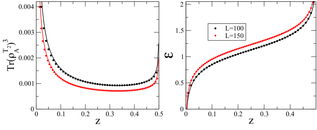
Refer to caption
Figure 8: A typical example of the entanglement of two adjacent intervals of the same length \ell in a periodic chain of length L𝐿L. The legend refers to both plots and we fix ω=106𝜔superscript106\omega=10^{-6}. Left: Tr(ρAT2)3Trsuperscriptsuperscriptsubscript𝜌𝐴subscript𝑇23{\rm Tr}(\rho_{A}^{T_{2}})^{3} as function of z=/L𝑧𝐿z=\ell/L. The data are consistent with the conformal prediction (full lines with only one multiplicative free parameter). Right: Logarithmic negativity {\cal E} for the same chains as on the left. Again the data are perfectly consistent with the CFT predictions (full lines with only one additive free parameter).

We now consider the case of two adjacent intervals in a periodic system of total length L𝐿L. For simplicity we consider the two intervals to have equal length \ell, thus all the results depend on the single parameter z/L[0,1/2]𝑧𝐿012z\equiv\ell/L\in[0,1/2]. In terms of z𝑧z, the CFT predictions in Eqs. (62) can be rewritten as (we fix c=1𝑐1c=1)

Tr(ρAT2)n{(sin(πz))(ne/22/ne)/3(sin(2πz))(ne/2+1/ne)/6,(sin2(πz)sin(2πz))(no1/no)/12,proportional-toTrsuperscriptsuperscriptsubscript𝜌𝐴subscript𝑇2𝑛casessuperscript𝜋𝑧subscript𝑛𝑒22subscript𝑛𝑒3superscript2𝜋𝑧subscript𝑛𝑒21subscript𝑛𝑒6missing-subexpressionmissing-subexpressionmissing-subexpressionsuperscriptsuperscript2𝜋𝑧2𝜋𝑧subscript𝑛𝑜1subscript𝑛𝑜12missing-subexpression{\rm Tr}(\rho_{A}^{T_{2}})^{n}\propto\left\{\begin{array}[]{ll}(\sin(\pi z))^{-(n_{e}/2-2/n_{e})/3}(\sin(2\pi z))^{-(n_{e}/2+1/n_{e})/6}\,,\\ \\ (\sin^{2}(\pi z)\sin(2\pi z))^{-(n_{o}-1/n_{o})/12},\end{array}\right. (200)

and the proportionality constants depend on L𝐿L in a known manner. For the logarithmic negativity from Eq. (63), we have

=14lnsin2(πz)sin(2πz)+cnst=14ln[tan(πz)]+cnst,14superscript2𝜋𝑧2𝜋𝑧cnst14𝜋𝑧cnst{\cal E}=\frac{1}{4}\ln\frac{\sin^{2}(\pi z)}{\sin(2\pi z)}+{\rm cnst}=\frac{1}{4}\ln[\tan(\pi z)]+{\rm cnst}\,, (201)

where again the additive constant depends on L𝐿L in a known manner. These predictions are checked against the numerical data in Fig. 8 where the only free parameters in each curve is fixed by a fit. The agreement is clearly excellent.
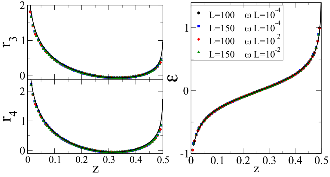
Refer to caption
Figure 9: Entanglement for two adjacent intervals of equal length <L/2𝐿2\ell<L/2 in a periodic chain of length L𝐿L. Left: the ratio rn(z)subscript𝑟𝑛𝑧r_{n}(z) in Eq. (202) as function of z=/L𝑧𝐿z=\ell/L compared with the parameter free CFT prediction. Right: Subtracted negativity ϵ(z)italic-ϵ𝑧\epsilon(z) in Eq. (205) again compared with the parameter free CFT prediction.

However one can do even better checks of the theory by constructing ratios in which all the dependence on non-universal parameters (such as those coming from the zero mode) and also the dependence on L𝐿L cancel. A straightforward idea would be to divide Tr(ρAT2)nTrsuperscriptsuperscriptsubscript𝜌𝐴subscript𝑇2𝑛{\rm Tr}(\rho_{A}^{T_{2}})^{n} for the value it assumes at a given fixed \ell, e.g. =L/4𝐿4\ell=L/4, i.e. by considering the logarithm of the ratio

rn(z)=lnTr(ρATA2=)nTr(ρATA2=L/4)n,subscript𝑟𝑛𝑧Trsuperscriptsuperscriptsubscript𝜌𝐴subscript𝑇subscript𝐴2𝑛Trsuperscriptsuperscriptsubscript𝜌𝐴subscript𝑇subscript𝐴2𝐿4𝑛r_{n}(z)=\ln\frac{{\rm Tr}(\rho_{A}^{T_{A_{2}=\ell}})^{n}}{{\rm Tr}(\rho_{A}^{T_{A_{2}=L/4}})^{n}}, (202)

whose parameter free CFT predictions for n𝑛n even and odd are

rne=16(2nene2)ln(2sin2(πz))16(ne2+1ne)ln(sin(2πz)),subscript𝑟subscript𝑛𝑒162subscript𝑛𝑒subscript𝑛𝑒22superscript2𝜋𝑧16subscript𝑛𝑒21subscript𝑛𝑒2𝜋𝑧\displaystyle r_{n_{e}}=\frac{1}{6}\Big{(}\frac{2}{n_{e}}-\frac{n_{e}}{2}\Big{)}\ln(2\sin^{2}(\pi z))-\frac{1}{6}\Big{(}\frac{n_{e}}{2}+\frac{1}{n_{e}}\Big{)}\ln(\sin(2\pi z))\,, (203)
rno=112(1nono)ln(2sin2(πz)sin(2πz)).subscript𝑟subscript𝑛𝑜1121subscript𝑛𝑜subscript𝑛𝑜2superscript2𝜋𝑧2𝜋𝑧\displaystyle r_{n_{o}}=\frac{1}{12}\Big{(}\frac{1}{n_{o}}-n_{o}\Big{)}\ln(2\sin^{2}(\pi z)\sin(2\pi z)). (204)

These ratios are shown in Fig. 9 for n=3𝑛3n=3 and n=4𝑛4n=4. The agreement of the numerical data and the CFT prediction is excellent. Some very small deviations are visible for z𝑧z close to 00 and 1/2121/2, but we checked that they go to zero increasing L𝐿L in a controllable way.

For the logarithmic negativity, we can analogously define the subtracted quantity

ϵ(z)=(,L)(L/4,L)=14ln[tan(πz)],italic-ϵ𝑧𝐿𝐿4𝐿14𝜋𝑧\epsilon(z)={\cal E}(\ell,L)-{\cal E}(L/4,L)=\frac{1}{4}\ln[\tan(\pi z)]\,, (205)

and again the rhs is a parameter free CFT prediction. In Fig. 9 (left panel), this prediction is compared with the numerical data and the agreement is extremely good since no deviations are visible even close to the boundaries.

7.6 The negativity for two disjoint intervals in the periodic chain.
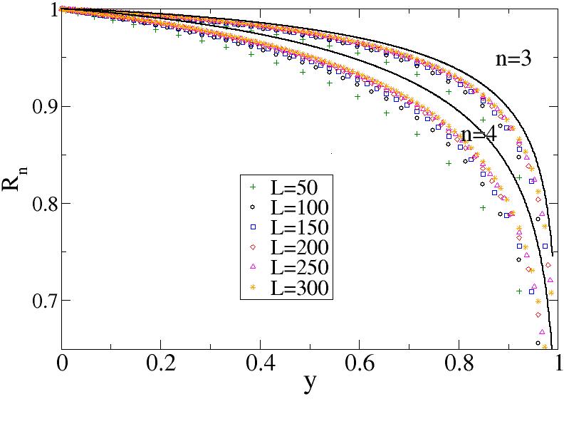
Refer to caption
Figure 10: For a periodic chain of length L𝐿L, we report the ratio Rn(y)subscript𝑅𝑛𝑦R_{n}(y) defined in Eq. (75) as function of y𝑦y for several L𝐿L and for n=3,4𝑛34n=3,4. The continuous lines are the parameter free CFT predictions to which the data converges for L𝐿L\to\infty.

To conclude our analysis of the periodic chain we consider now the most difficult situation of two disjoint intervals for which the negativity has been already considered numerically [12]. Here we start by considering the traces Tr(ρAT2)nTrsuperscriptsuperscriptsubscript𝜌𝐴subscript𝑇2𝑛{\rm Tr}(\rho_{A}^{T_{2}})^{n} which, in the conformal regime ωL1much-less-than𝜔𝐿1\omega L\ll 1, should be described by Eq. (72) with 𝒢n(y)subscript𝒢𝑛𝑦{\cal G}_{n}(y) given in (90). The direct numerical data, that we do not present here, agree well with the CFT predictions where the overall constant is fixed by a fit and explicitly depends on the values of ω𝜔\omega and L𝐿L, since the data are influenced by the zero mode. However, while this is a further confirmation of the predictive power of CFT, it gives not much information on the true entanglement (which is only obtained in the limit ne1subscript𝑛𝑒1n_{e}\to 1). Indeed the function 𝒢n(y)subscript𝒢𝑛𝑦{\cal G}_{n}(y) turns out to be very close to a constant (in proper units equals 1) and the direct data mainly probe the prefactor to 𝒢n(y)subscript𝒢𝑛𝑦{\cal G}_{n}(y) in Eq. (72), whose logarithm vanishes in the replica limit ne1subscript𝑛𝑒1n_{e}\to 1, and so does not give any contribution to the negativity.
Refer to caption
Figure 11: Finite size scaling analysis for dn(y)subscript𝑑𝑛𝑦d_{n}(y) in Eq. (206) for n=3𝑛3n=3 (left) and n=4𝑛4n=4 (right). We report from Fig. 10 several values of y𝑦y (increasing in the direction of the arrow, but we do not give the actual value to simplify the reading of the plot). The data are compatible with a leading correction to the scaling of the form L2/nsuperscript𝐿2𝑛L^{-2/n} .

As already stated in Sec. (5), a practical way to get rid of the prefactor is to consider the ratio Rn(y)subscript𝑅𝑛𝑦R_{n}(y) in Eq. (75), where also the non-universal parts due to the zero mode cancel and we are left with a universal function of y𝑦y. The CFT prediction for this ratio Rnη=(y)superscriptsubscript𝑅𝑛𝜂𝑦R_{n}^{\eta=\infty}(y) in Eq. (92) is compared to the numerical data in Fig. 10. As L𝐿L increases, the data approach the CFT result. The differences with the asymptotic formula are due to the presence of unusual corrections to the scaling [64, 65] whose leading part is of the form L2/nsuperscript𝐿2𝑛L^{-2/n}. A quantitative finite size scaling analysis is reported in Fig. 11 for n=3,4𝑛34n=3,4 showing that the difference

dn(y)Rn(y)Rnη=(y),subscript𝑑𝑛𝑦subscript𝑅𝑛𝑦superscriptsubscript𝑅𝑛𝜂𝑦d_{n}(y)\equiv R_{n}(y)-R_{n}^{\eta=\infty}(y), (206)

for several values of y𝑦y is of the expected form L2/nsuperscript𝐿2𝑛L^{-2/n}. As well known (even analytically) for other simpler cases [64, 66] for larger n𝑛n, the subleading corrections to the scaling, of the form L2p/nsuperscript𝐿2𝑝𝑛L^{-2p/n} with p𝑝p integer, cannot be neglected and a proper analysis requires the introduction of some fitting parameters.

Finally we turn to the study of the negativity {\cal E} reported in Fig.  12 showing that all data collapse on a single curve, without sizable corrections. Unfortunately we do not have the analytic continuation of Rneη=(y)superscriptsubscript𝑅subscript𝑛𝑒𝜂𝑦R_{n_{e}}^{\eta=\infty}(y) to ne1subscript𝑛𝑒1n_{e}\to 1 as a function of y𝑦y. However we can study the two interesting regimes of far and close intervals corresponding to y0𝑦0y\to 0 and y1𝑦superscript1y\to 1^{-} respectively. For small y𝑦y, the data, being very close to zero, are consistent with the prediction that they vanish faster than any power. In Ref. [12], on the basis of the numerical data, the form ea/ysuperscript𝑒𝑎𝑦e^{-a/\sqrt{y}} has been proposed. This proposal is shown in logarithmic scale on the inset of Fig. 12 together with a simple exponential eb/ysuperscript𝑒𝑏𝑦e^{-b/y}. The two possible scenarios are very difficult to be distinguished on the basis of the numerical calculations involving exponentially small numbers and the ambiguity can be resolved only by analytically continuing Rneη=(y)superscriptsubscript𝑅subscript𝑛𝑒𝜂𝑦R_{n_{e}}^{\eta=\infty}(y).

For y1𝑦1y\to 1, the general prediction from CFT (80) for c=1𝑐1c=1 is

(y)=14ln(1y)+,𝑦141𝑦{\cal E}(y)=-\frac{1}{4}\ln(1-y)+\dots\,, (207)

however, we have shown in Eq. (5.4.1) that for the model at hand, subleading double logarithmic corrections are present

(y)=14ln(1y)12lnK(y)lnP1+o(1),𝑦141𝑦12𝐾𝑦subscript𝑃1𝑜1{\cal E}(y)=-\frac{1}{4}\ln(1-y)-\frac{1}{2}\ln K(y)-\ln P_{1}+o(1)\,, (208)

where K(y)𝐾𝑦K(y) is the elliptic integral of the first kind and P1=0.832056subscript𝑃10.832056P_{1}=0.832056\dots is given in Eq. (120). Written in this form, the expansion contains also some of the subleading corrections (in 1y1𝑦1-y) and it is expected to describe the data better. Indeed in Fig. 12, this prediction is almost indistinguishable from the data all the way from y1similar-to𝑦1y\sim 1 (where it is an exact result) down to y0.3similar-to𝑦0.3y\sim 0.3. We should mention that the subleading logarithmic correction may be responsible for the exponent 1/3131/3 found in Ref. [12] as compared with our analytic result 1/4141/4.

Refer to caption
Figure 12: The negativity (y)𝑦{\cal E}(y) is a universal scale invariant function with an essential singularity at y=0𝑦0y=0. We report the data for L=50,100,150,200,250,300𝐿50100150200250300L=50,100,150,200,250,300 but, since they are hardly distinguishable, we do not give a legend box. The solid line is the expansion close to y1similar-to𝑦1y\sim 1 in Eq. (208) which very surprisingly describes well the data down to y0.3similar-to𝑦0.3y\sim 0.3. The inset shows the same plot in logarithmic scale showing that for small y𝑦y the two possibilities ea/ysimilar-tosuperscript𝑒𝑎𝑦{\cal E}\sim e^{-a/y} and eb/ysimilar-tosuperscript𝑒𝑏𝑦{\cal E}\sim e^{-b/\sqrt{y}} are too close to be distinguished.

Finally we would like to mention that, in a long enough chain, when each interval contains a finite number of lattice points, the negativity must vanish exactly for sufficiently large separations. Indeed the reduced density matrix ρAsubscript𝜌𝐴\rho_{A} has all strictly positive eigenvalues and in the limit when the intervals are far apart ρAsubscript𝜌𝐴\rho_{A} factorizes and each factor is a finite matrix with positive eigenvalues which become independent of the separation. Thus, when we take the partial transpose, the change in the density matrix, and therefore in the eigenvalues, can be made arbitrarily small since pipjdelimited-⟨⟩subscript𝑝𝑖subscript𝑝𝑗\langle p_{i}p_{j}\rangle (which is the correlator that changes sign, cf. Eq. (196)) decreases like |ij|2superscript𝑖𝑗2|i-j|^{-2}. Thus the partial transpose changes the elements of ρAsubscript𝜌𝐴\rho_{A} but an amount which is arbitrarily small so the eigenvalues do not change sign. Indeed this is consistent with the well-known result [1, 9] that the entanglement of two far away sites is exactly zero.

7.7 Tripartite chains with Dirichlet boundary in the origin

Now we consider the non-trivial case of a tripartite chain on a system with boundaries discussed in Sec. 6, which is the semi-infinite line, with A1=[0,]subscript𝐴10A_{1}=[0,\ell], A2=[,2]subscript𝐴22A_{2}=[\ell,2\ell] and B𝐵B the remainder. In this case, the results for Tr(ρAT2)nTrsuperscriptsuperscriptsubscript𝜌𝐴subscript𝑇2𝑛{\rm Tr}(\rho_{A}^{T_{2}})^{n} are given in Eq. (172) which we report also here:

Tr(ρAT2)n={c/6(n1/n)nodd,c/12(n1/n)c/6(n/22/n)neven.Trsuperscriptsuperscriptsubscript𝜌𝐴subscript𝑇2𝑛casessuperscript𝑐6𝑛1𝑛𝑛oddmissing-subexpressionmissing-subexpressionsuperscript𝑐12𝑛1𝑛𝑐6𝑛22𝑛𝑛even{\rm Tr}(\rho_{A}^{T_{2}})^{n}=\left\{\begin{array}[]{ll}\ell^{-c/6(n-1/n)}&n\;{\rm odd},\\ \\ \ell^{-c/12(n-1/n)-c/6(n/2-2/n)}&n\;{\rm even}.\end{array}\right. (209)

The most interesting feature is the peculiar behavior for n𝑛n even, which can be explicitly checked by considering the semi-infinite harmonic chain with ω=0𝜔0\omega=0. The results for the numerical evaluation of Tr(ρAT2)nTrsuperscriptsuperscriptsubscript𝜌𝐴subscript𝑇2𝑛{\rm Tr}(\rho_{A}^{T_{2}})^{n} are reported in Fig. 13 (left), showing the perfect agreement of both even and odd n=3,4,5,6𝑛3456n=3,4,5,6 where only the global amplitude has been fixed with a fit. The right panel of the same figure shows the corresponding logarithmic negativity which turns out to be described by the CFT prediction =1/4ln+limit-from14{\cal E}=1/4\ln\ell+ const.

Refer to caption
Figure 13: Tr(ρAT2)nTrsuperscriptsuperscriptsubscript𝜌𝐴subscript𝑇2𝑛{\rm Tr}(\rho_{A}^{T_{2}})^{n} (left) and logarithmic negativity (right) for a semi-infinite critical (ω=0𝜔0\omega=0) harmonic chain with Dirichlet boundary conditions in the origin. We report the results for two adjacent intervals of equal length l𝑙l with the first one starting from the origin. The data are perfectly described by the asymptotic CFT predictions reported as solid lines.

8 Some scaling considerations for massive theories

It is well known that for a gapped one-dimensional model, increasing \ell the entanglement (Rényi) entropy saturates to a finite value [30]. The calculation of this saturation value is generically complicated because it depends on microscopical details of the model and so it is calculable only for few simple integrable cases (see e.g. [22, 69, 70]). However, some general results can be worked out when a system is close to a conformal quantum critical point, and in the scaling limit where the lattice spacing a0𝑎0a\to 0 and with the correlation length fixed and large. Under these hypotheses and when all the lengths of the various subsystems (and so the total one for a finite system) are much larger than ξ𝜉\xi which is itself large, the Rényi entropies are [22]

SA(n)=𝒜c12(1+1n)logξa+O(ξ0),superscriptsubscript𝑆𝐴𝑛𝒜𝑐1211𝑛𝜉𝑎𝑂superscript𝜉0S_{A}^{(n)}={\cal A}\frac{c}{12}\Big{(}1+\frac{1}{n}\Big{)}\log\frac{\xi}{a}+O(\xi^{0})\,, (210)

where 𝒜𝒜{\cal A} is the number of boundary points between A𝐴A and its complement and c𝑐c is the central charge of the conformal field theory for ξ1=0superscript𝜉10\xi^{-1}=0. Clearly, when the interval lengths are of the order of ξ𝜉\xi, a complicated and universal (within the scaling limit) crossover takes place, which has been worked out only in very few QFT [22, 24, 71, 72].

The same difficulties for the entanglement entropy, with also some additional problems, make prohibitive the calculations of the negativity and Tr(ρAT2)nTrsuperscriptsuperscriptsubscript𝜌𝐴subscript𝑇2𝑛{\rm Tr}(\rho_{A}^{T_{2}})^{n} for a general gapped model. However, in the scaling limit and when the correlation length is itself large, but smaller than all the subsystems lengths, scaling considerations lead to very general results. For example in the case of a bipartition of a pure state in a finite interval of length ξmuch-greater-than𝜉\ell\gg\xi and the remainder, the scaling suggests to replace \ell with ξ𝜉\xi in Eqs. (48) and (49) for Tr(ρAT2)nTrsuperscriptsuperscriptsubscript𝜌𝐴subscript𝑇2𝑛{\rm Tr}(\rho_{A}^{T_{2}})^{n} and so the negativity is

=c2lnξ+O(ξ0).𝑐2𝜉𝑂superscript𝜉0{\cal E}=\frac{c}{2}\ln\xi+O(\xi^{0})\,. (211)

This is clearly true because it is the general relation (27) between negativity and Rényi entropy. A direct check of this is the general result for a bisected harmonic chain (i.e. A2subscript𝐴2A_{2} formed by N/2𝑁2N/2 consecutive sites and A1subscript𝐴1A_{1} the remainder) with periodic boundary conditions and nearest neighbor interaction. In this case, an interesting exact formula has been found for the logarithmic negativity [10]

=14ln(1+4KMω2),1414𝐾𝑀superscript𝜔2{\cal E}=\frac{1}{4}\ln\bigg{(}1+\frac{4K}{M\omega^{2}}\bigg{)}, (212)

which, remarkably, is independent of the size of the chain N𝑁N. In the limit ξ1ω1proportional-tosuperscript𝜉1𝜔much-less-than1\xi^{-1}\propto\omega\ll 1 gives =(lnξ)/2𝜉2{\cal E}=(\ln\xi)/2, in agreement with the general scaling.
Refer to caption
Figure 14: The negativity {\cal E} for two adjacent intervals of length =10,20,50102050\ell=10,20,50 (from bottom to top) in a periodic system of total length L=150𝐿150L=150. For ξ𝜉\xi\leq\ell all data collapse on the scaling prediction (213) while, when ξ𝜉\xi becomes of order \ell, a crossover to the CFT scaling form takes place.

A more interesting example can be obtained by considering the case of two adjacent intervals. Again, scaling suggests to substitute in Eq. (56) for the conformal case 1,2subscript12\ell_{1,2} with ξ𝜉\xi giving

=c4lnξ+O(ξ0).𝑐4𝜉𝑂superscript𝜉0{\cal E}=\frac{c}{4}\ln\xi+O(\xi^{0})\,. (213)

This scaling in ξ𝜉\xi is checked in Fig. 14 (left) for the harmonic chain for two adjacent intervals of the same length \ell. This shows an excellent agreement for 1ξmuch-less-than1𝜉much-less-than1\ll\xi\ll\ell while for larger ξ𝜉\xi, the crossover to the CFT prediction (56) takes place.

On the same lines as above, the negativity for other tripartitions can be deduced by means of simple scaling arguments.

9 Conclusions

We introduced a general field theoretical formalism to calculate the negativity and the logarithmic negativity, as an extension of our previous short communication [21]. This novel approach is based on a replica calculation of the traces of even integers nesubscript𝑛𝑒n_{e} powers of the partial transpose of the reduced density matrix and analytically continuing this to ne1subscript𝑛𝑒1n_{e}\to 1, i.e. the logarithmic negativity is

=limne1lnTr(ρAT2)ne.subscriptsubscript𝑛𝑒1Trsuperscriptsuperscriptsubscript𝜌𝐴subscript𝑇2subscript𝑛𝑒{\cal E}=\lim_{n_{e}\to 1}\ln{\rm Tr}(\rho_{A}^{T_{2}})^{n_{e}}\,. (214)

Several physical situations have been explicitly worked out for a conformally invariant theory:

  • The case in which A1subscript𝐴1A_{1} is an interval and A2subscript𝐴2A_{2} the remainder of an infinite, semi-infinite or finite (both periodic and with boundaries) system.

  • The case in which A1subscript𝐴1A_{1} and A2subscript𝐴2A_{2} are two adjacent intervals of length 1subscript1\ell_{1} and 2subscript2\ell_{2} respectively. For an infinite system the negativity is

    =c4ln121+2+cnst.𝑐4subscript1subscript2subscript1subscript2cnst{\cal E}=\frac{c}{4}\ln\frac{\ell_{1}\ell_{2}}{\ell_{1}+\ell_{2}}+{\rm cnst}\,. (215)

    This is simply generalized to a finite periodic system.

  • For the case in which A1subscript𝐴1A_{1} and A2subscript𝐴2A_{2} are two disjoint intervals (always of length 1subscript1\ell_{1} and 2subscript2\ell_{2}), the negativity turns out to depend on the full operator content of the theory and it is a scale invariant function (i.e. a function of the harmonic ratio of the four points defining the two intervals). We calculated the traces of integer powers of the partial transposed reduced density matrix for a free bosonic theory, both compactified (i.e. the Luttinger liquid field theory) and in the limit of infinite compactification radius. However, the n𝑛n dependence of these formulas is too complicated and we managed to calculate the analytic continuation only in some physical relevant limits (far and close intervals).

All the CFT results have been accurately checked for a chain of harmonic oscillators, finding perfect agreement. We also proposed a few scaling relations valid in the scaling regime when a theory is close to a conformal quantum critical point, and the correlation length (inverse gap or mass) is finite but large.

We are currently working out the generalization of the CFT approach to finite temperature field theories which is not as straightforward as it could naively appear. Finally, we mention that it is of extreme interest to check numerically all our CFT predictions in more complicated lattice models such as spin-chains and itinerant fermions described by the Luttinger liquid field theory, for which we worked out explicit predictions for Tr(ρAT2)nTrsuperscriptsuperscriptsubscript𝜌𝐴subscript𝑇2𝑛{\rm Tr}(\rho_{A}^{T_{2}})^{n} even in the case of disjoint intervals.

Acknowledgments

ET thanks Marcus Cramer for discussions. This work was supported by the ERC under Starting Grant 279391 EDEQS (PC). This work has been partly done when all the authors were guests of the Galileo Galilei Institute in Florence and Institut Henri Poincaré in Paris. ET thanks the Dipartimento di Fisica dell’Università di Pisa for the warm hospitality during the last part of this work.

References

References

  • [1] L Amico, R Fazio, A Osterloh, and V Vedral, Entanglement in many-body systems, Rev. Mod. Phys. 80, 517 (2008); J Eisert, M Cramer, and M B Plenio, Area laws for the entanglement entropy - a review, Rev. Mod. Phys. 82, 277 (2010); Entanglement entropy in extended systems, P Calabrese, J Cardy, and B Doyon Eds, J. Phys. A 42 500301 (2009).
  • [2] G. Vidal, Entanglement monotones, J. Mod. Opt. 47 (2000) 355.
  • [3] P. Calabrese and A. Lefevre, Entanglement spectrum in one-dimensional systems, Phys. Rev. A 78, 032329 (2008).
  • [4] M. B. Plenio and S. Virmani, An introduction to entanglement measures, Quant. Inf. Comput. 7, 1 (2007).
  • [5] F. Verstraete, J. J. Garcia-Ripoll, and J. I. Cirac, Matrix Product Density Operators: Simulation of finite-T and dissipative systems, Phys. Rev. Lett. 93, 207204 (2004); M. Zwolak and G. Vidal, Mixed-state dynamics in one-dimensional quantum lattice systems: a time-dependent superoperator renormalization algorithm, Phys. Rev. Lett. 93, 207205 (2004).
  • [6] J. Eisert and M. B. Plenio, A Comparison of entanglement measures, J. Mod. Opt.  46, 145 (1999).
  • [7] A. Peres, Separability criterion for density matrices, Phys. Rev. Lett.  77, 1413 (1996); M. Horodecki, P. Horodecki and R. Horodecki, Mixed state entanglement and distillation: Is there a ‘bound’ entanglement in nature?, Phys. Rev. Lett.  80, 5239 (1998); K. Zyczkowski, P. Horodecki, A. Sanpera and M. Lewenstein, On the volume of the set of mixed entangled states, Phys. Rev. A 58, 883 (1998); L. M. Duan, G. Giedke, J. I. Cirac and P. Zoeller, Inseparability criterion for continuos variables systems Phys. Rev. Lett.  84, 2722 (2000); R. Simon, Peres-Horodecki separability criterion for continuos variables systems Phys. Rev. Lett.  84, 2726 (2000).
  • [8] G. Vidal and R. F. Werner, A computable measure of entanglement, Phys. Rev. A 65, 032314 (2002).
  • [9] A. Osterloh, L. Amico, G. Falci, and R. Fazio, Scaling Properties of the Entanglement at a Quantum Phase Transition, Nature 416, 608 (2002).
  • [10] K. Audenaert, J. Eisert, M. B. Plenio and R. F. Werner, Entanglement Properties of the Harmonic Chain, Phys. Rev. A 66, 042327 (2002).
  • [11] H. Wichterich, J. Molina-Vilaplana, and S. Bose, Scale invariant entanglement at quantum phase transitions, Phys. Rev. A 80, 010304 (2009).
  • [12] S. Marcovitch, A. Retzker, M. B. Plenio, and B. Reznik, Critical and noncritical long range entanglement in the Klein-Gordon field, Phys. Rev. A 80, 012325 (2009).
  • [13] H. Wichterich, J. Vidal, and S. Bose, Universality of the negativity in the Lipkin-Meshkov-Glick model, Phys. Rev. A 81, 032311 (2010).
  • [14] A. Bayat, P. Sodano, and S. Bose, Negativity as the Entanglement Measure to Probe the Kondo Regime in the Spin-Chain Kondo Model, Phys. Rev. B 81, 064429 (2010).
  • [15] A. Bayat, S. Bose, P. Sodano, and H. Johannesson, Entanglement probe of two-impurity Kondo physics in a spin chain, Phys. Rev. Lett. 109, 066403 (2012).
  • [16] A. Bayat, P. Sodano, and S. Bose, Entanglement Routers Using Macroscopic Singlets, Phys. Rev. Lett. 105, 187204 (2010).
  • [17] P. Sodano, A. Bayat, and S. Bose Kondo Cloud Mediated Long Range Entanglement After Local Quench in a Spin Chain, Phys. Rev. B 81, 100412 (2010).
  • [18] J. Anders and A. Winter, Entanglement and separability of quantum harmonic oscillator systems at finite temperature Quant. Inf. Comput. 8, 245 (2008).
  • [19] J. Anders, Thermal state entanglement in harmonic lattices, Phys. Rev. A 77, 062102 (2008).
  • [20] A. Ferraro, D. Cavalcanti, A. Garcia-Saez, and A. Acin, Thermal bound entanglement in macroscopic systems and area laws, Phys. Rev. Lett. 100, 080502 (2008).
  • [21] P. Calabrese, J. Cardy, and E. Tonni, Entanglement negativity and quantum field theory, Phys. Rev. Lett. 109, 130502 (2012).
  • [22] P. Calabrese and J. Cardy, Entanglement entropy and quantum field theory, J. Stat. Mech. P06002 (2004).
  • [23] P. Calabrese and J. Cardy, Entanglement entropy and conformal field theory, J. Phys. A 42, 504005 (2009).
  • [24] J. L. Cardy, O.A. Castro-Alvaredo, and B. Doyon, Form factors of branch-point twist fields in quantum integrable models and entanglement entropy, J. Stats. Phys. 130 (2008) 129.
  • [25] F Gliozzi and L Tagliacozzo, Entanglement entropy and the complex plane of replicas, J. Stat. Mech. P01002 (2010).
  • [26] J. Kurchan, Replica trick to calculate means of absolute values: applications to stochastic equations, J. Phys. A 24, 4969 (1991).
  • [27] D. M. Gangardt and A. Kamenev, Replica Treatment of the Calogero-Sutherland Model, Nucl. Phys. B 610, 578 (2001); S. M. Nishigaki, D. M. Gangardt, and A. Kamenev, Correlation functions of the BC Calogero-Sutherland model, J. Phys. A 36, 3137 (2003); D. M. Gangardt, Universal correlations of trapped one-dimensional impenetrable bosons, J.Phys. A 37, 9335 (2004); D. M. Gangardt and G. V. Shlyapnikov, Off-diagonal correlations of lattice impenetrable bosons in one dimension, New J. of Phys. 8, 167 (2006); P. Calabrese and R. Santachiara, Off-diagonal correlations in one-dimensional anyonic models: A replica approach, J. Stat. Mech. P03002 (2009).
  • [28] M. Bianchi, G. Pradisi, and A. Sagnotti, Toroidal compactification and symmetry breaking in open string theories, Nucl.Phys. B 376, 365 (1992); see also chapter 6.4 of R. Blumenhagen and E. Plauschinn, Introduction to conformal field theory with application to string theory, Springer (2009).
  • [29] C. Holzhey, F. Larsen, and F. Wilczek, Geometric and renormalized entropy in conformal field theory, Nucl. Phys. B 424, 443 (1994); C. G. Callan and F. Wilczek, On geometric entropy. Phys. Lett. B 333, 55 (1994).
  • [30] G. Vidal, J. I. Latorre, E. Rico, and A. Kitaev, Entanglement in quantum critical phenomena, Phys. Rev. Lett. 90, 227902 (2003); J. I. Latorre, E. Rico, and G. Vidal, Ground state entanglement in quantum spin chains, Quant. Inf. Comp. 4, 048 (2004).
  • [31] M. Fagotti, P. Calabrese, and J. E. Moore, Entanglement spectrum of random-singlet quantum critical points, Phys. Rev. B 83, 045110 (2011).
  • [32] I. Affleck and A. W. W. Ludwig, Universal non-integer “ground-state degeneracy” in critical quantum systems, Phys. Rev. Lett. 67, 161 (1991).
  • [33] H.-Q. Zhou, T. Barthel, J. O. Fjaerestad, and U. Schollwoeck, Entanglement and boundary critical phenomena, Phys. Rev. A 74, 050305 (2006).
  • [34] P. Calabrese, J. Cardy, and E. Tonni, Entanglement entropy of two disjoint intervals in conformal field theory, J. Stat. Mech P11001 (2009).
  • [35] P. Calabrese, J. Cardy, and E. Tonni, Entanglement entropy of two disjoint intervals in conformal field theory II, J. Stat. Mech P01021 (2011).
  • [36] S. Furukawa, V. Pasquier, and J. Shiraishi, Mutual information and compactification radius in a c=1 critical phase in one dimension, Phys. Rev. Lett. 102, 170602 (2009).
  • [37] M. Caraglio and F. Gliozzi, Entanglement entropy and twist fields, JHEP 0811: 076 (2008).
  • [38] H. Casini, C. D. Fosco, and M. Huerta, Entanglement and alpha entropies for a massive Dirac field in two dimensions, J. Stat. Mech. P05007 (2005); H. Casini and M. Huerta, Remarks on the entanglement entropy for disconnected regions, JHEP 0903: 048 (2009); H. Casini and M. Huerta, Reduced density matrix and internal dynamics for multicomponent regions, Class. Quant. Grav. 26, 185005 (2009); H. Casini, Entropy inequalities from reflection positivity, J. Stat. Mech. (2010) P08019.
  • [39] P. Facchi, G. Florio, C. Invernizzi, and S. Pascazio, Entanglement of two blocks of spins in the critical Ising model, Phys. Rev. A 78, 052302 (2008).
  • [40] I. Klich and L. Levitov, Quantum noise as an entanglement meter, Phys. Rev. Lett. 102, 100502 (2009).
  • [41] V. Alba, L. Tagliacozzo, and P. Calabrese, Entanglement entropy of two disjoint blocks in critical Ising models, Phys. Rev. B 81 060411 (2010).
  • [42] V. Alba, L. Tagliacozzo, and P. Calabrese, Entanglement entropy of two disjoint intervals in c=1𝑐1c=1 theories, J. Stat. Mech. (2011) P06012.
  • [43] M. Fagotti and P. Calabrese, Entanglement entropy of two disjoint blocks in XY chains, J. Stat. Mech. (2010) P04016.
  • [44] P. Calabrese, Entanglement entropy in conformal field theory: New results for disconnected regions, J. Stat. Mech. (2010) P09013.
  • [45] F. Igloi and I. Peschel, On reduced density matrices for disjoint subsystems, 2010 EPL 89 40001.
  • [46] M. Headrick, Entanglement Renyi entropies in holographic theories, Phys. Rev. D 82, 126010 (2010).
  • [47] M. Fagotti, New insights into the entanglement of disjoint blocks, EPL 97, 17007 (2012).
  • [48] M. A. Rajabpour and F. Gliozzi, Entanglement entropy of two disjoint intervals from fusion algebra of twist fields, J. Stat. Mech. (2012) P02016.
  • [49] B. Swingle, Rényi entropy, mutual information, and fluctuation properties of Fermi liquids, Phys. Rev. B 86, 045109 (2012); P. Calabrese, M. Mintchev, and E. Vicari, Exact relations between particle fluctuations and entanglement in Fermi gases, EPL 98, 20003 (2012).
  • [50] J. Molina-Vilaplana and P. Sodano, Holographic View on Quantum Correlations and Mutual Information between Disjoint Blocks of a Quantum Critical System, JHEP 10 (2011) 011.
  • [51] S. Ryu and T. Takayanagi, Holographic derivation of entanglement entropy from AdS/CFT, Phys. Rev. Lett. 96 (2006) 181602; S. Ryu and T. Takayanagi, Aspects of holographic entanglement entropy, JHEP 0608: 045 (2006); V. E. Hubeny and M. Rangamani, Holographic entanglement entropy for disconnected regions, JHEP 0803: 006 (2008); M Headrick and T Takayanagi, A holographic proof of the strong subadditivity of entanglement entropy, Phys. Rev. D 76, 106013 (2007); T. Nishioka, S. Ryu, and T. Takayanagi, Holographic entanglement entropy: an overview, J. Phys. A 42 (2009) 504008; E. Tonni, Holographic entanglement entropy: near horizon geometry and disconnected regions, JHEP 1105:004 (2011).
  • [52] M. Headrick, A. Lawrence, and M. M. Roberts, Bose-Fermi duality and entanglement entropies, arXiv:1209.2428.
  • [53] A. Erderlyi, Higher transcendental functions, Mc Graw Hill, (1953).
  • [54] L. J. Dixon, D. Friedan, E. J. Martinec and S. H. Shenker, The Conformal Field Theory of Orbifolds, Nucl. Phys. B 282 (1987) 13.
  • [55] Al. B. Zamolodchikov, Conformal scalar field on the hyperelliptic curve and critical Ashkin-Teller multipoint correlation functions, Nucl. Phys. B 285 (1987) 481.
  • [56] R. Dijkgraaf, E. P. Verlinde and H. L. Verlinde, C = 1 Conformal Field Theories on Riemann Surfaces, Commun. Math. Phys.  115 (1988) 649.
  • [57] I. Peschel and M.-C. Chung, Density Matrices for a Chain of Oscillators, J. Phys. A 32, 8419 (1999); I. Peschel and V. Eisler, Exact results for the entanglement across defects in critical chains, J. Phys. A 45 (2012) 155301.
  • [58] I. Peschel, Calculation of reduced density matrices from correlation functions J. Phys. A 36, L205 (2003).
  • [59] A. Botero and B. Reznik, Spatial structures and localization of vacuum entanglement in the linear harmonic chain, Phys. Rev. A 70, 052329 (2004).
  • [60] M. B. Plenio, J. Eisert, J. Dreissig, and M. Cramer, Entropy, entanglement, and area: analytical results for harmonic lattice systems, Phys. Rev. Lett. 94, 060503 (2005); M. Cramer, J. Eisert, M. B. Plenio, and J. Dreissig An entanglement-area law for general bosonic harmonic lattice systems Phys. Rev. A 73 (2006) 012309.
  • [61] I. Peschel and V. Eisler, Reduced density matrices and entanglement entropy in free lattice models, J. Phys. A 42, 504003 (2009).
  • [62] S. Lievens, N. I. Stoilova and J. Van der Jeugt, Harmonic oscillator chains as Wigner Quantum Systems: Periodic and fixed wall boundary conditions in gl(1n)𝑔𝑙1𝑛gl(1-n) solutions, J. Math. Phys. 49 (2008) 073502.
  • [63] P. Di Francesco, P. Mathieu, and D. Senechal, Conformal Field Theory (Springer-Verlag, New York, 1997).
  • [64] P. Calabrese, M. Campostrini, F. Essler, and B. Nienhuis, Parity effects in the scaling of block entanglement in gapless spin chains, Phys. Rev. Lett. 104, 095701 (2010).
  • [65] J. Cardy and P. Calabrese, Unusual corrections to scaling in entanglement entropy, J. Stat. Mech. (2010) P04023.
  • [66] P. Calabrese and F. H. L. Essler, Universal corrections to scaling for block entanglement in spin-1/2 XX chains, J. Stat. Mech. (2010) P08029.
  • [67] J. L. Cardy, Conformal invariance and surface critical behaviour, Nucl. Phys. B 240, 514 (1984).
  • [68] M. Fagotti and P. Calabrese, Universal parity effects in the entanglement entropy of XX chains with open boundary conditions, J. Stat. Mech. P01017 (2011).
  • [69] A. R. Its, B.-Q. Jin, and V. E. Korepin, Entanglement in XY spin chain, J. Phys. A 38, 2975 (2005); F. Franchini, A. R. Its, and V. E. Korepin, Renyi entropy of the XY spin chain, J. Phys. A 41, 025302 (2008).
  • [70] I. Peschel, On the entanglement entropy for a XY spin chain, J. Stat. Mech. (2004) P12005; R. Weston, The Entanglement Entropy of Solvable Lattice Models, J. Stat. Mech. L03002 (2006); P. Calabrese, J. Cardy, and I. Peschel, Corrections to scaling for block entanglement in massive spin-chains, J. Stat. Mech. P09003 (2010); E. Ercolessi, S. Evangelisti, and F. Ravanini, Exact entanglement entropy of the XYZ model and its sine-Gordon limit, Phys. Lett. A 374, 2101 (2010).
  • [71] H. Casini and M. Huerta, Entanglement entropy in free quantum field theory, J. Phys. A 42, 504007 (2009); H. Casini and M. Huerta, Analytic results on the geometric entropy for free fields, J. Stat. Mech. P01012 (2008); H. Casini and M. Huerta Entanglement and alpha entropies for a massive scalar field in two dimensions, J. Stat. Mech. P12012 (2005).
  • [72] O. A. Castro-Alvaredo and B. Doyon, Bipartite entanglement entropy in massive 1+1-dimensional quantum field theories, J. Phys. A 42 504006 (2009); O. A. Castro-Alvaredo and B. Doyon, Bipartite entanglement entropy in massive QFT with a boundary: the Ising model J. Stat. Phys. 134, 105 (2009); B. Doyon, Bipartite entanglement entropy in massive two-dimensional quantum field theory, Phys. Rev. Lett. 102, 031602 (2009); O. A. Castro-Alvaredo and B. Doyon, Bipartite entanglement entropy in integrable models with backscattering, J. Phys. A 41 275203 (2008).