Forward particle correlations in the color glass condensate

Abstract

Multiparticle correlations, such as forward dihadron correlations in pA collisions, are an important probe of the strong color fields that dominate the initial stages of a heavy ion collision. We describe recent progress in understanding two-particle correlations in the dilute-dense system, e.g. at forward rapidity in deuteron-gold collisions. This requires evaluating higher point Wilson line correlators from the JIMWLK equation, which we find well described by a Gaussian approximation. We then calculate the dihadron correlation, including both the “elastic” and “inelastic” contributions, and show that our result includes the double parton scattering contribution.

1 Introduction

The physics of high energy hadronic or nuclear collisions is dominated by the gluonic degrees of freedom of the colliding particles. These small $x$ gluons form a dense nonlinear system that is, at high enough $\sqrt{s}$, best described as a classical color field and quantum fluctuations around it. The color glass condensate (CGC, for reviews see [1, *Weigert:2005us, *Gelis:2010nm, *Lappi:2010ek]) is an effective theory developed around this idea. It gives an universal description of the small $x$ degrees of freedom that can equally well be applied to small $x$ DIS as to dilute-dense (pA or forward AA) and dense-dense (AA or very high energy pp) hadronic collisions. The nonlinear interactions of the small $x$ gluons dynamically generate a new transverse momentum scale, the saturation scale $Q_{\mathrm{s}}$, that grows with energy. The scale $Q_{\mathrm{s}}$ dominates both the gluon spectrum and multiparton correlations.

The most convenient parametrization of the dominant gauge field is in terms of Wilson lines that describe the eikonal propagation of a projectile through it. The Wilson lines are drawn from a probability distribution, whose dependence on rapidity is described by the JIMWLK equation. This equation reduces, in a large ${N_{\mathrm{c}}}$ and mean field approximation, to the BK [5, *Kovchegov:1999yj] equation and further, in the dilute linear regime, to the BFKL one.

2 Correlations in a dilute-dense collision

Figure 1: Left: the JIMWLK result for the quadrupole correlator compared to the Gaussian approximation. Right: Comparison to the “naive large ${N_{\mathrm{c}}}$” approximation. Shown are the initial condition (MV model) at $y=0$ and the result after $5.18$ units of evolution in rapidity in the “line” coordinate configuration where $\mathbf{x}_{T}=\mathbf{u}_{T}$ and $\mathbf{y}_{T}=\mathbf{v}_{T}$. Figures from ref. [7].

One of the more striking signals of saturation physics at RHIC is seen in the relative azimuthal angle ($\Delta\varphi$) dependence of the dihadron correlation function, where the $\Delta\varphi\approx\pi$ back-to-back peak is seen to be suppressed in dAu-collisions compared to pp collisions at the same kinematics [8, 9]. The CGC description of this correlation starts from a large $x$ parton radiating a gluon, with subsequent eikonal propagation of the pair through the target. To calculate the matrix element for this process one needs target expectation values of products of Wilson line operators, such as the dipole and the quadrupole

$$\hat{D}(\mathbf{x}_{T},\mathbf{y}_{T})=\frac{1}{{N_{\mathrm{c}}}}\mathrm{Tr}U(\mathbf{x}_{T})U^{\dagger}(\mathbf{y}_{T})\quad\hat{Q}(\mathbf{x}_{T},\mathbf{y}_{T},\mathbf{u}_{T},\mathbf{v}_{T})=\frac{1}{{N_{\mathrm{c}}}}\mathrm{Tr}U(\mathbf{x}_{T})U^{\dagger}(\mathbf{y}_{T})U(\mathbf{u}_{T})U^{\dagger}(\mathbf{v}_{T}).$$ (1)

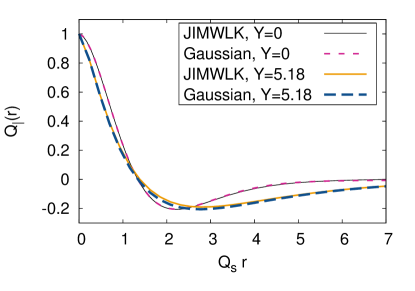
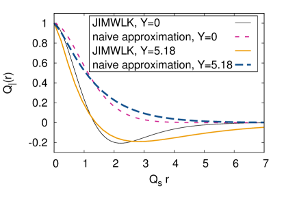
For practical phenomenological work it would be extremely convenient to be able to express these higher point correlators in terms of the dipole, which is straightforward to obtain from the BK equation. In the phenomenological literature so far [10] this has been done using a “naive large ${N_{\mathrm{c}}}$” (or “elastic”) approximation where the quadrupole is assumed to be simply a product of two dipoles. A more elaborate scheme would be a “Gaussian” approximation (“Gaussian truncation” in [11]), where one assumes the relation between the higher point functions and the dipole to be the same as in the (Gaussian) MV model. The expectation value of the quadrupole operator in the MV model has been derived e.g. in ref. [12].

In ref. [7] the validity of these approximations was studied by comparing them numerically to the solution of the JIMWLK equation. As studying the full 8-dimensional phase space for the quadrupole operator would be cumbersome, the numerical study was done in two special coordinate configurations. The most important results of ref. [7] is demonstrated in Fig. 1, with a comparison of the initial and evolved (for 5.18 units in $y$) JIMWLK results to the approximations. The MV-model initial condition $y=0$ satisfies the Gaussian approximation by construction, but the calculation shows that the Gaussian approximation is still surprisingly well conserved by the evolution. The naive large ${N_{\mathrm{c}}}$ approximation, on the other hand, fails already at the initial condition.

3 Dihadron correlation

This result does not yet fully address the effect on the measurable dihadron cross section. For that one must convolute a linear combination of Wilson line operators $\langle\hat{Q}\hat{D}\rangle,\langle\hat{D}\hat{D}\rangle$ and $\langle\hat{D}\rangle$ with the $q\to qg$ splitting wavefunction. For the explicit expressions we refer the reader to refs. [10, 15]. We have reported the outcome of this nontrivial numerical task in more detail in ref. [15].

Figure 2: Kinematics of the DPS limit. The double parton scattering contribution is obtained from the CGC dihadron cross section formula in the limit $n_{T}\to 0$.

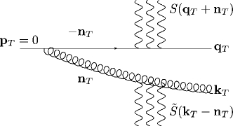
When using the full Gaussian correlator, instead of only the “elastic” term, one encounters an additional complication in the calculation, not encountered with the approximations used in refs. [10, 16]. In the limit of large distance, or small momentum, between the quark and the gluon, the operator $\langle\hat{Q}\hat{D}\rangle$ factorizes into a product of an adjoint and a fundamental representation dipole operator, describing the independent scattering of the quark and the gluon, respectively, off the target (see fig. 2). When this product is multiplied by the splitting wavefunction, the resulting integral is logarithmically infrared divergent. This divergence corresponds to a correlated quark-gluon pair being present in the incoming probe wavefunction, namely the double parton scattering (DPS) contribution discussed in this context in ref. [17]. For a consistent treatment it must be subtracted from the correlated cross section and calculated separately using an additional nonperturbative input describing the probe, a double parton distribution function.

Figure 3: A parton level comparison of the elastic approximation to our Gaussian approximation and its large ${N_{\mathrm{c}}}$ limit.

Figure 4: Illustration of the effect of the DPS contribution on the parton level: the dihadron yield divided by the $\Delta\varphi$-indpendent part.

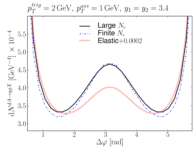
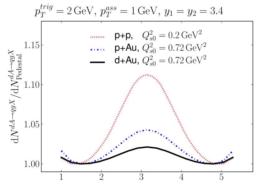
In fig. 4 we show the parton level dihadron production cross section obtained using different approximations for the quadrupole. We notice that the width and especially the height of the away side peak are modified when replacing the naive approximation, used e.g. in [10], by the Gaussian approximation [12]. In fig. 4 we show the yield divided by the $\Delta\varphi$-independent pedestal for pp, pAu and dAu collisions. The back-to-back correlation is suppressed for a nuclear target, due to the larger intrinsic transverse momentum $\sim Q_{\mathrm{s}}$. When the probe is switched from a proton to a deuteron, on the other hand, the correlated peak stays the same but the $\Delta\varphi$-independent background increases, resulting in a decreased ratio of the peak to the pedestal, shown in the plot. This is the effect discussed in much detail in ref. [17].

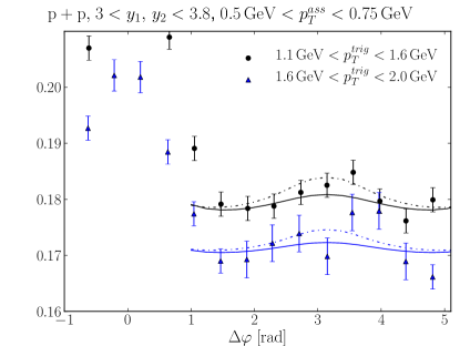
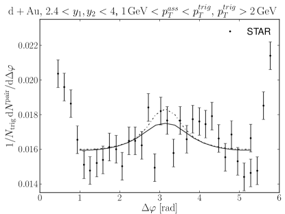
There is some remaining uncertainty in the normalization of the single inclusive spectrum (as evidenced by substantial K-factors needed in the literature to describe the single inclusive data), which propagates to a factor $\sim 2$ uncertainty in our estimates for the $\Delta\varphi$-independent pedestal. When comparing with PHENIX [8] data, we obtain for the trigger transverse momentum range $1.1\dots 1.6\textrm{ GeV}$ a pedestal $0.11\textrm{ GeV}^{-1}$, whereas the experimental value is $0.176\textrm{ GeV}^{-1}$. Similarly for the trigger transverse momentum $1.6\dots 2\textrm{ GeV}$ we obtain $0.08\textrm{ GeV}^{-1}$, and the experimental value reads $0.163\textrm{ GeV}^{-1}$. For the STAR [9] data our estimate for the pedestal is $0.02$ when the experimental value is $0.0145$. In order to compare to the experimental correlation peaks from the PHENIX and experiments we have adjusted this pedestal to the data. The resulting comparison is shown in fig. 5.

Figure 5: Comparison of our calculation to the PHENIX (left, [8]) and STAR (right, [9]) dihadron correlation data. The initial saturation scales are $Q_{\mathrm{s0}}^{2}=1.51\textrm{ GeV}^{2}$ (solid line) and $Q_{\mathrm{s0}}^{2}=0.72\textrm{ GeV}^{2}$ (dashed line).

Acknowledgements

H.M. is supported by the Graduate School of Particle and Nuclear Physics. This work has been supported by the Academy of Finland, project 133005 and by computing resources from CSC – IT Center for Science in Espoo, Finland.

References

- [1] E. Iancu and R. Venugopalan, The color glass condensate and high energy scattering in QCD, in Quark gluon plasma, edited by R. Hwa and X. N. Wang, World Scientific, 2003, arXiv:hep-ph/0303204
- [2] H. Weigert, Prog. Part. Nucl. Phys. 55, 461 (2005), [arXiv:hep-ph/0501087]
- [3] F. Gelis, E. Iancu, J. Jalilian-Marian and R. Venugopalan, Ann. Rev. Nucl. Part. Sci. 60, 463 (2010), [arXiv:1002.0333 [hep-ph]]
- [4] T. Lappi, Int. J. Mod. Phys. E20, 1 (2011), [arXiv:1003.1852 [hep-ph]]
- [5] I. Balitsky, Nucl. Phys. B463, 99 (1996), [arXiv:hep-ph/9509348]
- [6] Y. V. Kovchegov, Phys. Rev. D60, 034008 (1999), [arXiv:hep-ph/9901281]
- [7] A. Dumitru, J. Jalilian-Marian, T. Lappi, B. Schenke and R. Venugopalan, Phys. Lett. B706, 219 (2011), [arXiv:1108.4764 [hep-ph]]
- [8] PHENIX, A. Adare et al., Phys. Rev. Lett. 107, 172301 (2011), [arXiv:1105.5112 [nucl-ex]]
- [9] E. Braidot, arXiv:1102.0931 [nucl-ex]
- [10] J. L. Albacete and C. Marquet, Phys. Rev. Lett. 105, 162301 (2010), [arXiv:1005.4065 [hep-ph]]
- [11] J. Kuokkanen, K. Rummukainen and H. Weigert, Nucl. Phys. A875, 29 (2012), [arXiv:1108.1867 [hep-ph]]
- [12] F. Dominguez, C. Marquet, B.-W. Xiao and F. Yuan, Phys. Rev. D83, 105005 (2011), [arXiv:1101.0715 [hep-ph]]
- [13] E. Iancu and D. Triantafyllopoulos, JHEP 1111, 105 (2011), [arXiv:1109.0302 [hep-ph]]
- [14] E. Iancu and D. Triantafyllopoulos, JHEP 1204, 025 (2012), [arXiv:1112.1104 [hep-ph]]
- [15] T. Lappi and H. Mäntysaari, arXiv:1209.2853 [hep-ph]
- [16] A. Stasto, B.-W. Xiao and F. Yuan, Phys. Lett. B716, 430 (2012), [arXiv:1109.1817 [hep-ph]]
- [17] M. Strikman and W. Vogelsang, Phys. Rev. D83, 034029 (2011), [arXiv:1009.6123 [hep-ph]]