A Classical Framework for Nonlocality and Entanglement

Abstract

Based on our model of quantum systems as emerging from the coupled dynamics between oscillating “bouncers” and the space-filling zero-point field, a sub-quantum account of nonlocal correlations is given. This is explicitly done for the example of the “double two-slit” variant of two-particle interferometry. However, it is also shown that the entanglement in two-particle interferometry is only a natural consequence of the fact that already a “single” two-slit experiment can be described on a sub-quantum level with the aid of “entangling currents” of a generally nonlocal nature.

1 Introduction

Although nonlocality has featured very prominently throughout the last decades in the discussions on the foundations of quantum mechanics, no general consensus has yet been reached over it. Despite many arguments in favor of the position that nonlocal effects are one of the (if not the) main characteristics which distinguish classical from quantum mechanics, some researchers even hold on to the view that a purely local physics could suffice to explain all existing experimental data, thus ultimately relying on a familiar trait of classical physics.

However, even if one considered quantum mechanical nonlocality as a well-established fact, as we do, this does not necessarily mean that there cannot exist some form of “classical” explanation for it. In arguing for the use of modern, “21^st century classical physics”, our group, for example, has in recent years obtained with such classical means a series of results that were previously considered as obtainable only via quantum mechanics. Among these results, some features figure prominently, like, e.g., explanations of Planck’s postulate of energy quantization, the dispersion of a Gaussian, or interference at a double slit. (For an introduction, see Grossing.2012quantum and the references therein.) Thus, as a further task along our lines of reasoning, we intend in this paper to provide a classical framework for nonlocal effects and entanglement.

One of our main modeling scenarios is provided by the stimulating experiments of Couder’s group Couder.2005 ; Couder.2006single-particle ; Protiere.2006 ; Eddi.2009 ; Fort.2010path-memory , where “bouncing”, and also “walking”, droplets (the “particles”) are dynamically coupled to the oscillations of a bath (the “waves”) and thus produce a whole series of effects, which were previously considered only to be possible quantum mechanically. Among these effects, interference at a double slit, tunneling, or quantization of angular momentum in closed orbits could be reproduced, for example. Although it is clear that the mentioned experiments can only provide analogies, at best, one has here, nevertheless, a scenario providing essential stimuli for model building also in the context of quantum theory. This, at least, is what we want to propose here, i.e., that there are further insights to be gained from the experiments of Couder’s group, which could analogously be transferred into the modeling of quantum behavior. Concretely, we do believe that also an understanding of nonlocality and entanglement can profit from the study of said experiments. In fact, one indispensable prerequisite for these experiments to work, one basic commonality of all of them, is that the bath is vibrating itself. It so happens that bouncer and bath may engage in a self-organized, dynamically coupled entity where the bouncer can self-propel due to its interaction with the wave it generates.

In recent papers, we introduced an analogous scenario in the quantum domain, thereby having a particle/bouncer undergo also stochastic jumps such that diffusion theory can be applied. Then, what is in a quantum mechanical context described as a Gaussian wave-packet has an equivalent in the Gaussian distribution of a particle whose path follows the “agitations”, or “excitations”, of the underlying “bath”. With the latter, we refer in our model to the zero-point oscillations of the vacuum, i.e., something we take as empirically given, or, in other words, as an “ontological” input to our theory. Note that we completely agree here with Timothy Boyer who noted in a similar context:

“The concept of zero-point radiation (random radiation fluctuations at the zero of temperature) can appear in both classical and quantum theories. Zero-point radiation can not be regarded as belonging exclusively to quantum theory any more than the concepts of mass, energy, and gravity can be claimed as exclusively classical concepts because they appeared first in the context of classical mechanics.” Boyer.2010blackbody

As our model’s particle through its bouncing and locking-in with the zero-point field creates diffusion wave fields, and as the latter, at least in the nonrelativistic case, extend instantaneously along nonlocal distances Mandelis.2000diffusion ; Mandelis.2001structure ; Mandelis.2001diffusion-wave , we speak of a nonlocal “path excitation field”. Wherever the diffusion wave fields “radiated out” into the environment exist (or better: Wherever the bouncers’ oscillations lock in with the oscillations of the space-filling bath), the self-propelled bouncer (= “walker”) may go, eventually. So, in the case of a bouncer oscillating in some source region of an interferometer experiment, whenever it is propelled forward and can potentially go through one of the two slits, the (Gaussian) path excitation fields behind the double-slit will overlap to produce the familiar fringes at some screen Groessing.2012doubleslit . We stress, however, that one of the most important features of the path excitation field is its nonlocal nature. This is actually what we are going to work out in more detail in the present paper.

Apart from accepting as given the nonrelativistic diffusion wave fields’ “breathing” nonlocally throughout space, what could be a possible origin of the assumed nonlocal nature of the zero-point oscillations? One can only speculate at present, but it seems that a good candidate for an explanation would come from cosmological considerations. Note, for example, that for the universe in its initial phases, according to present-day models, one can admit, in addition to the particles existing in the very early universe, a set of phase-locked wave-like oscillations that would thus “resonate” throughout the whole small-scale universe. Then, it is conceivable that cosmic inflation, for example, would not destroy these oscillations, but rather “inflate” these fields as well, thus ending up with a much larger universe where the particles still oscillate in phase with the zero-point background, albeit with the latter now having turned a nonlocal one. Whatever the true reason for the nonlocality of the zero-point field may eventually be, we take the latter as an input for our modeling, and in the following show some results thereof.

2 A Sub-Quantum Kinematic Account of Two-Particle Correlations

Let us first consider an EPR-type experiment as it was proposed by Horne and Zeilinger Horne.1986einstein-podolsky-rosen for two-particle interferometry, i.e., essentially a “doubled” double-slit experiment as shown in Fig. 2.1. One creates a particle pair with equal but opposite momenta $\mathbf{k}_{1}$ and $\mathbf{k}_{2}$, respectively, along with some small changes $\delta\mathbf{k}$, which can be varied via phase shifters $\Phi_{1}$ and $\Phi_{2}$. Their quantum mechanical wave function would be described in terms of an entangled state. The resulting correlated intensity $I\left(\mathbf{x}_{1},\mathbf{x}_{2}\right)$ exhibits marked modulations, which persist even for arbitrarily large spatial separations of the individual particles’ wave packets.

Figure 2.1: Scheme of a two-particle interferometer, with the source S in the center emitting two anti-correlated particles, with different phase shifters $\Phi$ inserted into the particle beams, and with (possible locations of) detectors D.

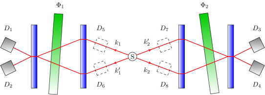
In our approach, we can make use of the path excitation field as follows. Each path $i$ be occupied by a Gaussian wave packet with a “forward” momentum $\mathbf{p}_{i}=\hbar\mathbf{k}_{i}=m\mathbf{v}_{i}$. (Moreover, due to the stochastic process of path excitation, the latter is represented also by a large number of consecutive Brownian shifts, $\mathbf{p}_{u,\alpha}=m\mathbf{u}_{\alpha}$, but we shall return to this only in the next chapter, where we shall discuss in more detail the different roles played by the velocity fields $\mathbf{v}$ and $\mathbf{u}$, respectively.) To start with, we note first the probability density currents for each “particle”, and then combine them in a suitable manner. Thus, upon preparation of the two-particle source, we start with some initial distribution $P\left(\mathbf{x}_{0},\,t_{0}\right)=R_{0}^{2}\left(\mathbf{x}_{0},\,t_{0}\right)$ of a composite system just at decay time $t_{0}$. Considered as a two-particle system, and since we employ a wave theory, this initial distribution can be rewritten as $P\left(\mathbf{x}_{0},\,t_{0}\right)=R_{L}\left(\mathbf{x}_{0},\,t_{0}\right)R_{R}\left(\mathbf{x}_{0},\,t_{0}\right)$, with $R_{L}$ and $R_{R}$ signifying normalized amplitudes associated with particles going left (locations $\mathbf{x}_{1}$) or right (mirror locations $\mathbf{x}_{2}$), respectively. This initial distribution is thus split up into one channel for particle $1$ and a correspondingly anti-correlated channel for particle $2$ (Fig. 2.1). Note that, because each of the two bouncers “excites” the areas in both directions (i.e., both possible paths) of the surrounding medium, the probability density for each path is given by $P\left(\mathbf{x}_{i},\,t\right)=R_{L}\left(\mathbf{x}_{i},\,t\right)R_{R}\left(\mathbf{x}_{i},\,t\right)$, for $i=1$ or $2$, and similarly for the primed quantities, where $R_{L}$ and $R_{R}$ now more specifically refer to the amplitudes “excited” by the bouncer going left or right, respectively, irrespective of which actual particle one focuses upon. For simplicity, we shall in the examples below concentrate on the symmetric scenario with equal weights, i.e., $R_{L}\left(\mathbf{x}_{1}\right)=R_{R}\left(\mathbf{x}_{1}\right)=R_{L}\left(\mathbf{x}_{2}\right)=R_{R}\left(\mathbf{x}_{2}\right)$.

Then, in close similarity to our treatment of the case of a single double-slit Groessing.2012doubleslit , for the “doubled” setup we write down the total average probability current as the sum of all four average probability currents present, i.e., firstly without the presence of any phase shifters it holds (with bars denoting averages) that

$$\overline{\mathbf{J}}_{\textrm{tot}}=P_{{\rm tot}}\overline{\mathbf{v}}_{{\rm tot}}=P_{{\rm tot}}\frac{\hbar}{m}\overline{\mathbf{k}}_{{\rm tot}}:=\frac{\hbar}{m}\left[R_{L}R_{R}\mathbf{\overline{k}}_{1}+R_{L}R_{R}\mathbf{\overline{k}}_{2}+R_{L}^{\prime}R_{R}^{\prime}\mathbf{\overline{k}}_{1}^{\prime}+R_{L}^{\prime}R_{R}^{\prime}\mathbf{\overline{k}}_{2}^{\prime}\right].$$ (2.1)

Allowing now for a relative phase $\varphi=\Phi_{1}-\Phi_{2}$ through the insertion of the phase shifters $\Phi_{1}$ and $\Phi_{2}$, one can write with the “total” average momenta $\mathbf{\overline{k}}:=\mathbf{\overline{k}}_{1}+\mathbf{\overline{k}}_{2}$ and $\mathbf{\overline{k}^{\prime}}:=\mathbf{\overline{k}}_{1}^{\prime}+\mathbf{\overline{k}}_{2}^{\prime}+\overline{\mathbf{\delta k}}$, respectively,

$$P_{\mathrm{tot}}\overline{\mathbf{k}}_{\mathrm{tot}}=\left[R_{L}R_{R}\left(\mathbf{\overline{k}}_{1}+\mathbf{\overline{k}}_{2}\right)+R_{L}^{\prime}R_{R}^{\prime}\left(\mathbf{\overline{k}}_{1}^{\prime}+\mathbf{\overline{k}}_{2}^{\prime}+\overline{\mathbf{\delta k}}\right)\right].$$ (2.2)

Then we obtain with normalization $\mathfrak{\mathsf{\mathcal{N}}}$, with the momentum balance $k_{\mathrm{tot}}=k=k^{\prime}$, and with hats denoting average unit vectors, the correlated intensity

$$I\left(\mathbf{x}_{1},\mathbf{x}_{2}\right):=\mathcal{N}^{2}P_{\mathrm{tot}}^{2}\left(\mathbf{x}_{1},\mathbf{x}_{2}\right)=\mathcal{N}^{2}\left[R_{L}R_{R}\mathbf{\hat{k}}+R_{L}^{\prime}R_{R}^{\prime}\mathbf{\hat{k}}^{\prime}\right]^{2},$$ (2.3)

and thus

$$I\left(\mathbf{x}_{1},\mathbf{x}_{2}\right)= \mathcal{N}^{2}\left[\vphantom{\int_{0}^{0}}R_{L}^{2}R_{R}^{2}+R_{L}^{\prime 2}R_{R}^{\prime 2}\right.$$

$$+\left.2R_{L}R_{R}R_{L}^{\prime}R_{R}^{\prime}\cos\left\{\left[\left(\mathbf{\overline{k}}_{1}+\mathbf{\overline{k}}_{2}\right)-\left(\mathbf{\overline{k}}_{1}^{\prime}+\mathbf{\overline{k}}_{2}^{\prime}+\overline{\mathbf{\delta k}}\right)\right]\cdot\mathbf{r}\right\}\vphantom{\int_{0}^{0}}\right].$$ (2.4)

This is the exact quantum mechanical result, albeit here obtained without invoking the quantum mechanical calculus. Moreover, one can now also highlight particular features of this remarkable correlation along nonlocal distances $r=x_{1}+x_{2}$ between the locations $\mathbf{x}_{1}$ and $\mathbf{x}_{2}$, respectively. Namely, as opposed to the formula (2.4) derived from the total probability density current, one can also single out correlations between individual currents, respectively, for the various channels. An important role is thereby played by the relative phase $\varphi$, which emerges naturally in our model as it relates a “bouncer’s” oscillations along different paths Groessing.2012doubleslit ; Groessing.2013dice .

As is usual in interferometry, differences in relative phase are – also classically – accounted for by phase shifts of $\frac{\pi}{2}$ for each reflection of a beam at one of the slabs of the interferometer. Thus, by comparing primed versus unprimed scenarios, one can for example relate the intensities at detectors $D_{2}$ and $D_{4}$ in Fig. 2.1, which provide the conditional probability

$$P\left(D_{2}\left|D_{4}\right.\right)= \mathcal{N}^{2}R_{L}^{2}R_{R}^{2}\left[\vphantom{\int_{0}^{0}}2+2\cos\left\{\left[\left(\mathbf{\overline{k}}_{1}+\mathbf{\overline{k}}_{2}\right)-\left(\mathbf{\overline{k}}_{1}^{\prime}+\mathbf{\overline{k}}_{2}^{\prime}+\overline{\mathbf{\delta k}}\right)\right]\cdot\mathbf{r}\right\}\right]$$

$$= \frac{1}{4}\left(2+2\cos\left[\Phi_{1}-\Phi_{2}\right]\right)=\frac{1}{2}\left(1+\cos\varphi\right),$$ (2.5)

whereas

$$P\left(D_{2}\left|D_{3}\right.\right)=\frac{1}{4}\left(2+2\cos\left[\Phi_{1}-\Phi_{2}+\pi\right]\right)=\frac{1}{2}\left(1-\cos\varphi\right).$$ (2.6)

However,

$$P\left(D_{6}\left|D_{4}\right.\right)=\frac{1}{4}\left(2+2\cos\frac{\pi}{2}\right)=\frac{1}{2},$$ (2.7)

for example, because the phase difference between the two possible paths is now independent of the $\Phi_{i}$ and given by $\varphi=\frac{\pi}{2}$. From the latter example one sees that an “early” detection of a particle at $D_{6}$, which is equivalent to a which-way measurement, or to the “closing of the second slit” on one side of a double-double-slit experiment, respectively, destroys nonlocal interference effects such as those indicated by (2.5) or (2.6).

How can we understand this behavior in our model? Now, we have mentioned on several occasions that we consider the Gaussians employed in our calculations as simple solutions of a diffusion equation. More generally, however, as has been explicated in the works of Mandelis et al. Mandelis.2000diffusion ; Mandelis.2001structure ; Mandelis.2001diffusion-wave , diffusion wave fields related to oscillating sources may in a more specific way extend nonlocally across the whole domain of an experimental setup, for example. Thus, the Gaussians used so far may be only approximations to more complex solutions of the diffusion equation, which actually may exhibit long wiggly tails, albeit with very small amplitudes. However, it is exactly such a functional characteristic which has been found also in a specific quantum mechanical context, i.e., for example, in Rauch’s post-selection experiments Rauch.2006hidden ; Rauch.2012particle . There, it turned out that for interference to occur it is not necessary that the “main bulks” (approximated by Gaussians) of wave-packets overlap. Rather, the experiments show that interference can be caused by the nonlocally far-reaching action of the plane-waves of a quantum mechanical wave-function. This is actually the corollary of our understanding of the nonlocal nature of the zero-point field to which our particle/oscillator couples: A Gaussian indicating the approximate whereabouts of our bouncer, embedded in an oscillatory “bath” of momentum fluctuations, the regular part of which thereby coinciding with the action of the plane-wave components in quantum mechanics.

Note particularly that the bandwidth of these plane-wave components is determined by the momentum resolution of the whole measurement apparatus, where the upper limit is defined by the inverse of the distance between source and detector Rauch.2012particle . This is strongly reminiscent of our analogy with the particle’s bounces in the Couder experiments, which are locked-in with the oscillations of the fluid. The spatial constraints of the latter, i.e., the container sizes, thus define the momentum resolution of the experiment via a suitable bandwidth of possible wavelengths. So, we observe that in our model it is the wholeness of the possible wave configurations within the possibly nonlocal limits of an experimental setup that co-determines the experiments’ outcomes.

In other words, whenever the “constraints” of the experimental setup are changed, this may have a nonlocal effect on the registered particles – a possibility which brings us back to the effect of the “closing of a slit” in the double-slit experiment. Note that, as this effect is shown in a forthcoming paper Groessing.2013dice to be essentially nonlocal, it is of the same nature as the one in EPR-type experiments, as, for example, in Aspect’s experiments: As opposed to mere kinematic nonlocality like the one implied by intensity correlations such as (2.4), we are in ref. Groessing.2013dice interested in the effects of the actual “closing of a slit”, i.e., in dynamic nonlocality Tollaksen.2010quantum . However, in the present paper we shall restrict our discussion to the simple double-slit experiment. For this alone already suffices to bring forth essential features of nonlocality and entanglement: The classical roots of entanglement are already visible in the “single” double-slit experiment, as will be shown now.

3 Entangling Currents in the Double-Slit Experiment

We consider the particles as emerging from one of two “Gaussian slits”, i.e., two possible paths of a particle which later eventually cross each other. To do so, we started in Groessing.2012doubleslit with an independent numerical computation of two Gaussian wave packets, with the total distribution given by

$$P_{{\rm tot}}:=P_{1}+P_{2}+2\sqrt{P_{1}P_{2}}\cos\varphi_{12}\,,$$ (3.1)

Figure 3.1: Classical computer simulation of the interference pattern in a double-slit experiment; with $v_{x,1}=-v_{x,2}$.

Figure 3.2: Same as Fig. 3.1, with an additional phase $\Delta\varphi=\pi$ at slit 1.

Figure 3.3: Classical computer simulation of the total average “entangling current” density in a double-slit experiment; same setup as in Fig. 3.1, with arbitrary normalization and $v_{x,1}=-v_{x,2}$.

Figure 3.4: Same as Fig. 3.3, with an additional phase shift of $\Delta\varphi=\pi$ at slit 1 according to the setup of Fig.3.2. Comparing with Fig. 3.3, one notes that the dramatic shift from maxima to minima, and vice versa, as observed in the interference patterns of Fig. 3.1 and Fig.3.2, respectively, is essentially caused by the changes in these entangling currents.

where the phase difference

$$\varphi_{12}=\varphi_{2}-\varphi_{1}=\frac{1}{\hbar}\left[m(v_{2}-v_{1})x+\frac{mu_{0}^{2}}{2}\left(\frac{(x-x_{02}-v_{2}t)^{2}-(x-x_{01}-v_{1}t)^{2}}{\sigma^{2}(t)}\right)t\right]$$ (3.2)

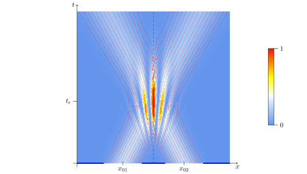
is characterized by the usual “classical” velocity difference $v_{2}-v_{1}$and a kinetic energy term including a momentum fluctuation $mu_{0}$, or the “osmotic” velocity $u_{0}$, respectively. Here, we indicate the two slits at positions $x_{01}$ and $x_{02}$ and we assume the same slit widths and hence the same initial standard deviations $\sigma_{0}$. The graphical result of a classical computer simulation of the interference pattern in a double-slit experiment, including the average trajectories, with evolution from bottom to top, is shown in Fig. 3.1. The Gaussian wave packets characterized by moderate spreading at the same standard deviations $\sigma$ move towards each other with velocities $v_{x,1}=-v_{x,2}$. One can observe a basic characteristic of the averaged particle trajectories, which, only because of the averaging, are identical with the Bohmian trajectories. To fully appreciate this characteristic, we remind the reader of the severe criticism of Bohmian trajectories as put forward by Scully and others (see Scully.1998bohm , and references therein). We can note that in our sub-quantum approach an explanation of the obvious “no crossing rule” is straightforward and actually a consequence of a detailed microscopic momentum conservation. In Fig. 3.1 the maximum of the resulting distribution is positioned along the central symmetry line in between the two slits. Groessing.2012doubleslit

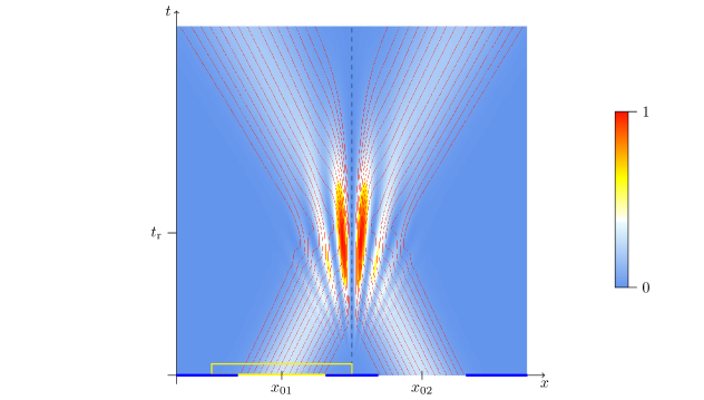
The interference hyperbolas for the maxima characterize the regions where the phase difference $\varphi_{12}=2n\pi$, and those with the minima lie at $\varphi_{12}=(2n+1)\pi$, $n=0,\pm 1,\pm 2,\ldots$ Note in particular the “kinks” of trajectories moving from the center-oriented side of one relative maximum to cross over to join more central (relative) maxima. In our classical explanation of double slit interference, a detailed “micro-causal” account of the corresponding kinematics is given. (For the details, see Groessing.2012doubleslit .) Since each Gaussian has its own phase distribution (3.2), we are free to add a phase shift $\Delta\varphi$ at one of the two slits, say slit 1, which modifies $\varphi_{1}$ to

$$\varphi_{1}=\frac{S_{1}}{\hbar}+\Delta\varphi.$$ (3.3)

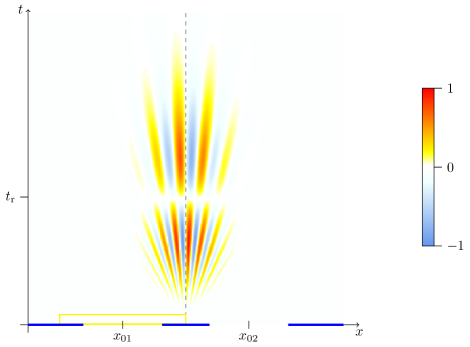
In Fig. 3.2, we use the same double-slit arrangement as in Fig. 3.1, but now include a phase shifter affecting slit 1, as sketched by the yellow rectangle on the left hand side. The exemplary choice of $\Delta\varphi=\pi$ results in a shift of the interference fringes. Comparing with Fig. 3.1, we recognize now a minimum of the resulting distribution along the central symmetry line.

Finally, we reconsider our classically obtained total average probability current Grossing.2012quantum ; Groessing.2012doubleslit

$$J_{{\rm tot}}=P_{1}v_{1}+P_{2}v_{2}+\sqrt{P_{1}P_{2}}\left(v_{1}+v_{2}\right)\cos\varphi_{12}+\sqrt{P_{1}P_{2}}\left(u_{1}-u_{2}\right)\sin\varphi_{12}\,,$$ (3.4)

with osmotic velocities $u_{i}$ and convective velocities $v_{i}$ applied to both slits, $i=1$ and 2, and with the phases (3.2) and (3.3).

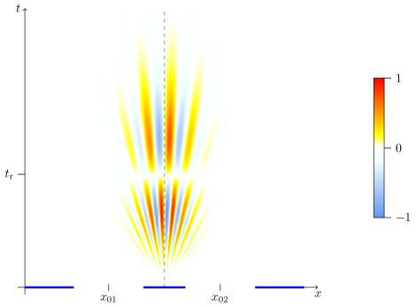
The result of our computer simulation of Eq. (3.4) is shown in Figs. 3.3 and 3.4 corresponding to the intensity distributions of Figs. 3.1 and 3.2, respectively. One recognizes the change of the maximum values of the probability current along the central symmetry line in Fig. 3.4 in comparison with those of Fig. 3.3. Since the figures display the one-dimensional case, the current flow is along the $x$–axis only. Interestingly, at the time $t_{{\rm r}}$ of the reversal of the trajectories, the current flow comes to a hold, and starts again for times $t>t_{{\rm r}}$ with reversed signs. This can be understood as a reversal of the relative flow of heat $Q_{2}-Q_{1}$ between the two channels, since $u_{i}=-\frac{1}{2\omega m}\nabla Q_{i}$ Groessing.2009origin , such that the last term of Eq. (3.4) reads as $\frac{1}{2\omega m}\sqrt{P_{1}P_{2}}\nabla(Q_{2}-Q_{1})\sin\varphi_{12}$.

The probability current $J_{{\rm tot}}$ in both figures essentially only consists of the last term of Eq. (3.4), as the velocities $v_{i}$ and the velocities $u_{i}$ typically differ by many orders of magnitude. In other words, the probability current $J_{{\rm tot}}$ is always dominated by the “quantum mechanical” entangling term of Eq. (3.4) which is connected to the osmotic velocities, $u_{1}$ and $u_{2}$, and which implies the existence of nonlocal correlations. As we have just seen, this “entangling current” can also be understood as describing the “heat flow” between the two channels. Note that, as opposed to the average total probability current $J_{{\rm tot}}$, in the distribution (3.1) of the probability density $P_{{\rm tot}}$ alone, just as in the correlated intensity (2.4) of two-particle interferometry, the entangling part is not explicitly visible.

The phenomenon of entanglement is thus possibly rooted in the existence of the path excitation field, a version of which we already encountered in the present paper with the usual double-slit interference.

In other words, one can say that the entanglement characteristic for two-particle interferometry is a natural consequence of the fact demonstrated here, i.e., that already in single-particle interferometry one deals with entangling currents, which generally are of a nonlocal nature.

References

- (1) G. Grössing, S. Fussy, J. Mesa Pascasio, and H. Schwabl, “The Quantum as an Emergent System,” J. Phys.: Conf. Ser. 361 (2012) 012008, arXiv:1205.3393v1.
- (2) Y. Couder, S. Protière, E. Fort, and A. Boudaoud, “Dynamical phenomena: Walking and orbiting droplets,” Nature 437 (2005) 208–208.
- (3) Y. Couder and E. Fort, “Single-particle Diffraction and Interference at a macroscopic scale,” Phys. Rev. Lett. 97 (2006) 154101.
- (4) S. Protière, A. Boudaoud, and Y. Couder, “Particle-wave association on a fluid interface,” J. Fluid Mech. 554 (2006) 85–108.
- (5) A. Eddi, E. Fort, F. Moisy, and Y. Couder, “Unpredictable Tunneling of a Classical Wave-Particle Association,” Phys. Rev. Lett. 102 (2009) 240401.
- (6) E. Fort, A. Eddi, A. Boudaoud, J. Moukhtar, and Y. Couder, “Path-memory induced quantization of classical orbits,” PNAS 107 (2010) 17515 –17520.
- (7) T. H. Boyer, “Blackbody Radiation and the Scaling Symmetry of Relativistic Classical Electron Theory with Classical Electromagnetic Zero-Point Radiation,” Found. Phys. 40 (2010) 1102–1116.
- (8) A. Mandelis, “Diffusion Waves and their Uses,” Phys. Today 53 (2000) 29–34.
- (9) A. Mandelis, “Structure and the Reflectionless/Refractionless Nature of Parabolic Diffusion-Wave Fields,” Phys. Rev. Lett. 87 (2001) 020801.
- (10) A. Mandelis, Diffusion-wave fields: Mathematical methods and Green functions. Springer, New York, NY, 2001.
- (11) G. Grössing, S. Fussy, J. Mesa Pascasio, and H. Schwabl, “An explanation of interference effects in the double slit experiment: Classical trajectories plus ballistic diffusion caused by zero-point fluctuations,” Ann. Phys. 327 (2012) 421–437, arXiv:1106.5994v3.
- (12) M. A. Horne and A. Zeilinger, “Einstein-Podolsky-Rosen Interferometry,” in New Techniques and Ideas in Quantum Measurement Theory, D. M. Greenberger, ed., vol. 480 of Annals of the New York Academy of Sciences, pp. 469–474. New York Academy of Sciences, New York, 1986.
- (13) G. Grössing, S. Fussy, J. Mesa Pascasio, and H. Schwabl, “Emergence of Dynamical Nonlocality from Changing Constraints on Sub-Quantum Kinematics,” to be published (2013) .
- (14) H. Rauch, M. Baron, S. Filipp, Y. Hasegawa, H. Lemmel, and R. Loidl, “Hidden observables in neutron quantum interferometry,” Physica B 385–386, Part 2 (2006) 1359–1364.
- (15) H. Rauch, “Particle and/or wave features in neutron interferometry,” J. Phys.: Conf. Ser. 361 (2012) 012019.
- (16) J. Tollaksen, Y. Aharonov, A. Casher, T. Kaufherr, and S. Nussinov, “Quantum interference experiments, modular variables and weak measurements,” New J. Phys. 12 (2010) 013023, arXiv:0910.4227v1.
- (17) M. O. Scully, “Do Bohm Trajectories Always Provide a Trustworthy Physical Picture of Particle Motion?,” Phys. Scr. T76 (1998) 41–46.
- (18) G. Grössing, “On the thermodynamic origin of the quantum potential,” Physica A 388 (2009) 811–823, arXiv:0808.3539v1.