Turku Centre for Quantum Physics, Department of Physics and Astronomy, University of Turku, FI-20014 Turku, Finland
Dipartimento di Matematica, Politecnico di Milano, Piazza Leonardo da Vinci 32, I-20133 Milano, Italy
Foundations of quantum mechanics; measurement theory
Comparing the degrees of incompatibility inherent in probabilistic physical theories
Abstract
We introduce a new way of quantifying the degrees of incompatibility of two observables in a probabilistic physical theory and,
based on this, a global measure of the degree of incompatibility inherent in such theories, across all observable pairs.
This opens up a novel and flexible way of comparing
probabilistic theories with respect to the nonclassical feature of incompatibility, raising many interesting questions, some of which
will be answered here. We show that quantum theory contains observables that are as incompatible as any probabilistic physical
theory can have if arbitrary pairs of observables are considered. If one adopts a more refined measure of the degree of incompatibility, for instance,
by restricting the comparison to binary observables, it turns out that there are probabilistic theories whose inherent degree
of incompatibility is greater than that of quantum mechanics.
To be published in: Europhysics Letters (2013).
pacs:
03.65.TaQuantum theory has a number of important features not known in classical physics, ranging from the superposition and indeterminacy principles formulated by the pioneers to the more recently discovered no-cloning and no-broadcasting theorems. It is an old problem to identify operationally significant properties of quantum theory that distinguish it from other probabilistic theories. In recent years many features have been under intensive investigation from this perspective, including information processing [1], optimal state discrimination [2], entropy [3], purification [4] and discord [5]. It has been found that some properties are quite generally valid in any non-classical (no-signaling) probabilistic theories while others are specifically quantum.
The existence of pairs of incompatible observables marks one of the most striking distinctions between quantum theory and classical physical theories. There are many manifestations of incompatibility, perhaps the most famous being the Heisenberg uncertainty principle [6]. However, there are many nonclassical probabilistic theories which also possess incompatible observables, and it will be of interest to compare quantum theory with alternative theories with respect to the feature of incompatibility.
To this end, we define the joint measurability region of any given pair of observables in a probabilistic theory. The joint measurability region describes the amount of added noise needed to make the observables jointly measurable. The global joint measurability feature of a probabilistic theory can then be characterized as the intersection of all the joint measurability regions associated with the theory.
We demonstrate that quantum theory contains observables that are as incompatible as observables in any probabilistic theory can be. Hence, we can say that, in a global sense, quantum theory has as great a degree of incompatibility as any other probabilistic theory. But if only binary observables are considered, the degree of incompatibility inherent in quantum theory is limited and we give an example of a probabilistic theory that contains maximally incompatible binary observables.
Our aim is thus to compare the incompatibility of pairs of observables in different probabilistic physical theories. We first need to set some minimal constraints.
A probabilistic theory is a framework that provides
a description of physical systems in terms of states and observables with the following general properties:
(i) The states of a system are represented by the elements of a convex subset
of a real vector space.
(ii) An observable is represented as an affine mapping from the set of states into the set of probability distributions
on some outcome space.
For simplicity, we restrict ourselves here to observables with a finite or countable number of outcomes.
(iii)
Any affine mapping from the set of states into the set of probability distributions is a valid observable.
We consider a particular probabilistic theory (PT) as given by a family of convex sets of states with associated sets of observables that share some properties specific to that PT. One may think of each pair consisting of a set of states with associated set of observables as an instance of a PT representing a particular type of physical system.
Given a PT, we denote by the probability of obtaining a measurement outcome when an observable is measured in a state . Hence, and . We will typically label the measurement outcomes by integers.
In quantum theory the states are described by density operators and observables correspond to POVMs [7]. Their duality is given by the trace formula (with a density operator and a POVM)
| (1) |
Another example of a probabilistic theory is a classical theory, where the states are probability measures on a phase space and observables are traditionally represented as functions ; the associated affine maps from states to probability distributions are then given by the formula
| (2) |
Continuing our discussion on general probabilistic theories, we note that it follows from the required properties (i)-(iii) that the set of observables is a convex set; a mixture of two observables is an observable. Physically mixing corresponds to an experiment where we switch between two measurement apparatuses with a random probability. We can directly write a mixture of two observables with the same set of measurement outcomes. If the sets of measurement outcomes differ, we can still write a mixture by first adding enough outcomes and then embedding both sets into .
Another consequence of the basic requirements is that every constant mapping , where is a fixed probability distribution, is an observable and we call it a trivial observable. A trivial observable corresponds to a dice rolling experiment, where we randomly pick the measurement outcome according to a given fixed probability distribution, without manipulating the state at all. In quantum theory, trivial observables are described by POVMs such that each operator is a multiple of the identity operator, i.e., for some with .
The concept of joint measurement can be defined in any probabilistic theory. Two observables and are jointly measurable if there exists an observable such that
| (3) |
In this case is called a joint observable of and . If and are not jointly measurable, then we say that they are incompatible.
Any probabilistic theory contains jointly measurable pairs of observables. Namely, a trivial observable is jointly measurable with any other observable; we can write a joint observable
| (4) |
for the trivial observable and any other observable . This simply corresponds to an experiment where we measure and simultaneously roll a dice. It is a well known fact that, in quantum theory, an observable which is jointly measurable with all other observables is necessarily a trivial observable. Indeed, any POVM element of such an observable commutes with all projections and must therefore be a scalar multiple of the identity (e.g. [8, Theorem IV.1.3.1]).
The following simple observation is a key ingredient for our discussion.
Proposition 1.
Let and be two observables and . Then and are jointly measurable for any choice of trivial observables and .
This proposition can be proved with the following construction. First, let and be the probability distributions related to and . We define an observable by formula
| (5) |
For a fixed , the right hand side is clearly a probability distribution. Moreover, the right hand side is an affine mapping on ; therefore is an observable. The marginal observables are
This proves Prop. 1.
The physical idea behind this construction is the following. In each measurement run we flip a coin and, depending on the result, we measure either or in the input state . In this way we get a measurement outcome for either or . In addition to this, we roll a dice and pretend that this is a measurement outcome for the other observable. In this way we get an outcome for both observables simultaneously. The overall observable is the one given in formula (5).
For two observables and , we denote by the set of all points for which there exist trivial observables such that and are jointly measurable, and we call the joint measurability region of and . The joint measurability region thus characterizes how much noise (in terms of trivial observables) we need to add to obtain jointly measurable approximations of and . Clearly, and are jointly measurable if and only if .
The joint measurability region is a convex region which can be plotted in the plane. To see this, let and , then we have to show that for . Thus let and be jointly measurable, and similarly for and , with suitable choices of trivial observables. Then the observables and are jointly measurable [9, Prop. 2].
Note that according to Prop. 1 the line . Moreover, it is trivially the case that . The convexity of then entails that the convex hull of the three points , and is in , hence we have:
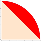
As an example, suppose that we are within quantum theory and and correspond to spin- measurements in two orthogonal directions, say and -axes. We then describe them with two POVMs and , where
| (6) |
and are the usual Pauli matrices in . It has been shown in [10] that for the uniformly distributed trivial observable (hence describing an unbiased coin), the two observables and are jointly measurable if and only if . It is also known [9, Prop. 3] that this inequality is a necessary condition for the joint measurability of any pair and , where are arbitrary trivial observables. Therefore, we conclude that
| (7) |
This region is depicted in Fig. 1.
In addition to describing the incompatibility of pairs of observables, the concept of a joint measurability region also provides a means to compare the degrees of incompatibility inherent in entire theories. A global joint measurability feature of a probabilistic theory PT is characterized by the intersection of all the sets across all instances of PT, and we denote
| for all pairs of observables and | |||
We call the joint measurability region for . We always have , but can be larger than . The larger the surplus region is, the more jointly measurable the theory is globally; see Fig. 2. If , this means that there is a pair of observables and such that the mixtures and are incompatible with any choice of trivial observables and .
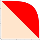
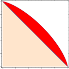
Since can be defined in any probabilistic theory, we can compare the joint measurability regions for different theories. We obviously have in any probabilistic theory where all measurements are jointly measurable, such as the classical probability theory. In the case of the greatest degree of incompatibility we would have . We will next show that quantum theory incorporates, globally, as much incompatibility between pairs of observables as a probabilistic theory can do.
Theorem 1.
In quantum theory . In particular, for any probabilistic theory PT.
In quantum theory every observable corresponds to a unique POVM by equation (1). We will prove that for any pair , there are quantum observables and such that the mixtures and are incompatible with any choice of trivial observables . Our proof is based on a recent result [11] on the joint measurability region for two complementary observables, which is a generalization of the result illustrated in Fig. 1.
Proof of Theorem 1.
We have earlier seen that , so we need to show that . Let , i.e., . Fix such that . We then choose to be a positive integer satisfying
| (8) |
(This can be done since the left hand side when .) We will consider a quantum system that is described by a -dimensional Hilbert space . Let be an orthonormal basis for . We define another orthonormal basis for by
| (9) |
The orthonormal bases and are mutually unbiased, i.e., . We define two POVMs and by
| (10) |
We thus obtain a pair of -outcome observables on . Since and consist of projections and , it follows that they are incompatible.
As proved in [11], the observables and are incompatible for any choice of trivial observables whenever
| (11) |
Since
| (12) |
we conclude that . ∎
Using the ideas of the proof of Theorem 1, we can also show that the conclusion can be reached by using a single pair of incompatible observables if we consider an infinite dimensional system and observables with a countably infinite number of outcomes.
Let be an infinite dimensional Hilbert space and write it as a direct sum of finite -dimensional Hilbert spaces , . In each consider a pair of mutually unbiased orthonormal bases and , where the latter is obtained from the first one by the formula (9). We define two POVMs and via
| (13) |
These observables act in the infinite dimensional Hilbert space and in (13) is an index labeling the different outcomes. The outcome space of and is .
Theorem 2.
The observables and defined in (13) satisfy .
Proof of Theorem 2.
Let and be two probability distributions defined on . Assume that and define two observables via
| (14) |
We need to show that and are incompatible. To prove this, we make the counter assumption that are jointly measurable. This implies that for any projection on , the projected observables and acting on a subspace are jointly measurable. (If is a joint observable of two observables , then is a joint observable of in .) Especially, the projections of and to any subspace should be jointly measurable. But from the result cited in the proof of Theorem 1 we know that for large enough, the projections to are incompatible. Hence, and are incompatible. ∎
We note that the observables and defined in (13) are not the only pair satisfying . Namely, we can modify and in any chosen subspace but the conclusion is still true since it depends on the fact that and contain mutually unbiased bases in arbitrarily high dimension.
An interesting problem within quantum theory would be to try to find a characterization of all pairs of quantum observables that satisfy . In particular, we may ask if maximally incompatible observables can exist in a finite dimensional Hilbert space, or if they can have a finite number of outcomes. Since two mutually unbiased bases are expected to be among the most incompatible observable pairs in a fixed dimension , our construction in the proof of Theorem 1 suggests that the answer to the first question would be negative. A proof of this claim is, however, lacking.
As for the second question, we can present a partial answer by investigating the joint measurability region in the case of pairs of binary quantum observables. Our aim is to show that
for any binary observables and , regardless of the dimension of the Hilbert space. In other words, we will show that two orthogonal spin observables are as incompatible as any binary observables can be.
To this end, let us note that two binary quantum observables are incompatible if and only if they enable a violation of the Bell-CHSH inequality [12]. We must therefore look at the Bell expression
Let us denote and . By [13, Theorem 1], there exist unit vectors such that for ; and conversely, given any quadruple of unit vectors there exist a corresponding set of binary observables and a bipartite state such that this equality holds. In particular, we have and so that an application of the Cauchy-Schwarz inequality along with the parallelogram law yields
By choosing the unit vectors appropriately we also see that any pair satisfying this condition can be obtained.
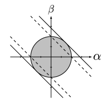
If we now mix the observables with the trivial observable with some weights and we see that the pair turns into , thus changing the Bell expression from to . We must therefore determine those for which for all satisfying (see Fig. 3). But the boundary curve for this region is obtained when the equations and have at most one common solution. By inserting into the first equation the problem reduces to determining when the discriminant is negative or zero, and one readily verifies that this is the case exactly when .
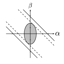
In conclusion, given any pair of binary observables and , and weights and with , the mixtures and can not be used to violate the Bell-CSHS inequality and must therefore be jointly measurable. We note that in the case the same result using a different technique has been obtained by Banik et al. [14].
Although Theorem 2 shows that quantum theory contains pairs of observables that are maximally incompatible, the strictly larger joint measurability region when restricting to binary observables suggests that more fine grained quantifications of the global degree of incompatibility between observables might not rank quantum theory among the most extreme theories in this respect. The example below will show that when restricting to just binary observables, it is indeed possible for a theory to have the smallest possible joint measurability region. In that sense such a theory must be considered to embody a strictly greater degree of incompatibility than quantum theory.
Consider any probabilistic theory, which contains a state space isomorphic to a square, by which we mean the convex hull of four different points in satisfying , for instance and . We will show that there is a pair of binary observables which are maximally incompatible. Let and be binary observables that pick out the right and top sides of the square respectively, i.e.
| (15) |
Proposition 2.
For the binary observables and defined in (15), .
Proof.
Suppose that there exists a joint observable for and where and are trivial observables. Let and be the probability distributions associated to and so that we have for any state
Any satisfying such marginal properies will be correctly normalised, but to be a valid observable, all the components of must take positive values on the points . In particular, we must have
Rewriting the last of these inequalities and invoking the defining property on the gives
where the final step comes about from invoking the positivity of on . ∎
The result of Proposition 2 does not come as a surprise in light of the fact that the barrier to maximal incompatibility of binary quantum observables comes from the connection with a Bell-CHSH inequality. Indeed, square shaped state spaces have been used in a model of a probabilistic theory containing the PR boxes which violate such an inequality to its maximal possible value.
We note that the conclusion of Proposition 2 is not restricted to the square state space. Consider any state space containing a square whose vertices are extreme points of the state space and whose boundary lines lie on the boundary of the state space; assume further that opposite sides of the square are contained in parallel hyperplanes that do not intersect with the interior of the state space. These two pairs of hyperplanes define effects whose values on the satisfy Eq. (15). It follows that the proof of Proposition 2 can be adopted in such cases. Examples are given by state space of the following shapes: pyramid, double pyramid, cube, cylinder.
The fact that the restriction to just binary observables allows one to differentiate between probabilistic theories that both contain maximally incompatible observables suggests that a more fine grained global measure of the degree of incompatibility is needed if the aim is to pick out a single theory as the one containing overall the most incompatible pairs of observables. For instance, for a given probabilistic theory PT we may define to be the joint measurability region for all possible -outcome observables in PT. Since increasing the number of outcomes of observables by simply adding outcomes that never occur does not change the properties of incompatibility, we immediately have . By comparing the regions in different theories for different values of we obtain a more fine grained way of comparing the degrees of incompatibility within the theories. It may even turn out that in this sense quantum theory embodies globally the least amount of incompatibility among the theories containing maximally incompatible observables. However, this is still an open question and a topic for future investigations.
Acknowledgements. The authors wish to thank Tom Bullock for comments on an earlier version of this paper. T.H. and J.S. acknowledge financial support from the Academy of Finland (grant no. 138135). J.S. also acknowledges financial support from the Italian Ministry of Education, University and Research (FIRB project RBFR10COAQ). N.S. gratefully acknowledges support through the award of an Annie Currie Williamson PhD Bursary at the University of York. Finally, the authors wish to thank an anonymous referee for suggesting a number of improvements to the presentation of the material.
References
- [1] J. Barrett, Phys. Rev. A, 75 (2007) 032304.
- [2] G. Kimura, T. Miyadera, H. Imai, Phys. Rev. A, 79 (2009) 062306.
- [3] H. Barnum, J. Barrett, L. Orloff Clark, M. Leifer, R. Spekkens, N. Stepanik, A. Wilce, R. Wilke, New J. Phys., 12 (2010) 033024.
- [4] G. Chiribella, G.M. D’Ariano, P. Perinotti, Phys. Rev. A, 84 (2011) 012311.
- [5] P. Perinotti, Phys. Rev. Lett., 108 (2012) 120502.
- [6] P. Busch, T. Heinonen, P. Lahti. Phys. Rep., 452 (2007) 155.
- [7] P. Busch, M. Grabowski, P.J. Lahti, Operational Quantum Physics, Springer-Verlag, Berlin, 1997. 2nd. corr. printing.
- [8] G. Ludwig, Foundations of Quantum Mechanics I, Springer-Verlag, Berlin, 1983.
- [9] P. Busch T. Heinosaari, Quant. Inf. Comp., 8 (2008) 0797.
- [10] P. Busch, Phys. Rev. D, 33 (1986) 2253.
- [11] C. Carmeli, T. Heinosaari, A. Toigo, Phys. Rev. A, 85 (2012) 012109.
- [12] M.M. Wolf, D. Perez-Garcia, C. Fernandez, Phys. Rev. Lett., 103 (2009) 230402.
- [13] B.S. Cirel’son, Lett. Math. Phys.,4 (1980) 93.
- [14] M. Banik, Md.R. Gazi, S. Ghosh, G. Kar, Phys. Rev. A 87 (2013) 052125.