Unbiased Risk Estimates for Singular Value Thresholding
and Spectral Estimators

Abstract

In an increasing number of applications, it is of interest to recover an approximately low-rank data matrix from noisy observations. This paper develops an unbiased risk estimate—holding in a Gaussian model—for any spectral estimator obeying some mild regularity assumptions. In particular, we give an unbiased risk estimate formula for singular value thresholding (SVT), a popular estimation strategy which applies a soft-thresholding rule to the singular values of the noisy observations. Among other things, our formulas offer a principled and automated way of selecting regularization parameters in a variety of problems. In particular, we demonstrate the utility of the unbiased risk estimation for SVT-based denoising of real clinical cardiac MRI series data. We also give new results concerning the differentiability of certain matrix-valued functions.

Keywords. Singular value thresholding, Stein’s unbiased risk estimate (SURE), differentiability of eigenvalues and eigenvectors, magnetic resonance cardiac imaging.

1 Introduction

Suppose we have noisy observations ${\bm{Y}}$ about an $m\times n$ data matrix ${\bm{X}}^{0}$ of interest,

$$Y_{ij}=X^{0}_{ij}+W_{ij},\qquad W_{ij}\stackrel{{\scriptstyle\text{iid}}}{{\sim}}\mathcal{N}(0,\tau^{2}),\quad\begin{array}[]{l}i=1,\ldots,m,\\ j=1,\ldots,n.\end{array}$$ (1.1)

We wish to estimate ${\bm{X}}^{0}$ as accurately as possible. In this paper, we are concerned with situations where the estimand has some structure, namely, ${\bm{X}}^{0}$ has low rank or is well approximated by a low-rank matrix. This assumption is often met in practice since the columns of ${\bm{X}}^{0}$ can be quite correlated. For instance, these columns may be individual frames in a video sequence, which are typically highly correlated. Another example concerns the acquisition of hyperspectral images in which each column of ${\bm{X}}^{0}$ is a 2D image at a given wavelength. In such settings, images at nearby wavelengths typically exhibit strong correlations. Hence, the special low-rank regression problem (1.1) occurs in very many applications and is the object of numerous recent studies.

Recently, promoting low-rank has been identified as a promising tool for denoising series of MR images, such as those that arise in functional MRI (fMRI) [34], relaxometry [22], cardiac MRI [36], NMR spectroscopy [5, 25], and diffusion-weighted imaging [15, 24], among others. In dynamic applications like cine cardiac imaging, where “movies” of the beating heart are created, neighboring tissues tend to exhibit similar motion profiles through time due to their physical connectedness. The diversity of temporal behaviors in this settings will, by nature, be limited, and the Casorati matrix (a matrix whose columns comprise vectorized frames of the image series) formed from this data will be low-rank [17]. For example, in breath-hold cine cardiac imaging, background tissue is essentially static and the large submatrix of the Casoratian corresponding to this region is very well approximated by a rank-1 matrix.

1.1 Singular value thresholding

Whenever the object of interest has (approximately) low rank, it is possible to improve upon the naive estimate $\hat{{\bm{X}}}_{0}={\bm{Y}}$ by regularizing the maximum likelihood. A natural approach consists in truncating the singular value decomposition of the observed matrix ${\bm{Y}}$, and solve

$$\mathrm{SVHT}_{\lambda}({\bm{Y}})=\arg\min_{{\bm{X}}\in\mathbb{R}^{m\times n}}\frac{1}{2}\|{\bm{Y}}-{\bm{X}}\|_{F}^{2}+\lambda\,\operatorname{rank}({\bm{X}}),$$ (1.2)

where $\lambda$ a positive scalar. As is well known, if

$${\bm{Y}}={\bm{U}}{\bm{\Sigma}}{\bm{V}}^{*}=\sum_{i=1}^{\min(m,n)}\sigma_{i}{\bm{u}}_{i}{\bm{v}}_{i}^{*}$$ (1.3)

is a singular value decomposition for ${\bm{Y}}$, the solution is given by retaining only the part of the expansion with singular values exceeding $\lambda$,

$$\mathrm{SVHT}_{\lambda}({\bm{Y}})=\sum_{i=1}^{\min(m,n)}\mathbb{I}(\sigma_{i}>\lambda)\,{\bm{u}}_{i}{\bm{v}}_{i}^{*}.$$

In other words, one applies a hard-thresholding rule to the singular values of the observed matrix ${\bm{Y}}$. Such an estimator is discontinuous in ${\bm{Y}}$ and a popular alternative approach applies, instead, a soft-thresholding rule to the singular values:

$$\mathrm{SVT}_{\lambda}({\bm{Y}})=\sum_{i=1}^{\min(m,n)}(\sigma_{i}-\lambda)_{+}\,{\bm{u}}_{i}{\bm{v}}_{i}^{*};$$ (1.4)

that is, we shrink the singular values towards zero by a constant amount $\lambda$. Here, the estimate $\mathrm{SVT}_{\lambda}({\bm{Y}})$ is Lipschitz continuous. This follows from the fact that the singular value thresholding operation (1.4) is the prox of the nuclear norm $\|\cdot\|_{*}$ (the nuclear norm of a matrix is sum of its singular values), i.e. is the unique solution to

$$\text{min}\quad\frac{1}{2}\|{\bm{Y}}-{\bm{X}}\|_{F}^{2}+\lambda\|{\bm{X}}\|_{*}.$$ (1.5)

The focus of this paper is on this smoother estimator referred to as the singular value thresholding ($\mathrm{SVT}$) estimate.

1.2 A SURE formula

The classical question is, of course, how much shrinkage should be applied. Too much shrinkage results in a large bias while too little results in a high variance. To find the correct trade-off, it would be desirable to have a method that would allow us to compare the quality of estimation for different values of the parameter $\lambda$. Ideally, we would like to select $\lambda$ as to minimize the mean-squared error or risk

$$\text{MSE}(\lambda)=\operatorname{\mathbb{E}}\|{\bm{X}}^{0}-\mathrm{SVT}_{\lambda}({\bm{Y}})\|_{F}^{2}.$$ (1.6)

Unfortunately, this cannot be achieved since the expectation in (1.6) depends on the true ${\bm{X}}^{0}$, and is thus unknown. Luckily, when the observations follow the model (1.1), it is possible to construct an unbiased estimate of the risk, namely, Stein’s Unbiased Risk Estimate (SURE) [32] given by

$$\textsc{SURE}(\mathrm{SVT}_{\lambda})({\bm{Y}})=-mn\tau^{2}+\sum_{i=1}^{\min(m,n)}\min(\lambda^{2},\sigma_{i}^{2})+2\tau^{2}\mathrm{div}\,(\mathrm{SVT}_{\lambda}({\bm{Y}})),$$ (1.7)

where $\{\sigma_{i}\}_{i=1}^{n}$ denote the singular values of ${\bm{Y}}$. Above, ‘$\mathrm{div}$’ is the divergence of the nonlinear mapping $\mathrm{SVT}_{\lambda}$, which is to be interpreted in a weak sense. Roughly speaking, it can fail to exist on negligible sets. The main contribution of this paper is to provide a closed-form expression for the divergence of this estimator. We prove that in the real-valued case,

$$\mathrm{div}\,(\mathrm{SVT}_{\lambda}({\bm{Y}}))=\sum_{i=1}^{\min(m,n)}\left[\mathbb{I}(\sigma_{i}>\lambda)+|m-n|\left(1-\frac{\lambda}{\sigma_{i}}\right)_{+}\right]+2\sum_{i\neq j,i,j=1}^{\min(m,n)}\frac{\sigma_{i}(\sigma_{i}-\lambda)_{+}}{\sigma_{i}^{2}-\sigma_{j}^{2}},$$ (1.8)

when ${\bm{Y}}$ is simple—i.e., has no repeated singular values—and $0$ otherwise, say, is a valid expression for the weak divergence. Hence, this simple formula can be used in (1.7), and ultimately leads to the determination of a suitable threshold level by minimizing the estimate of the risk, which only depends upon the observed data.

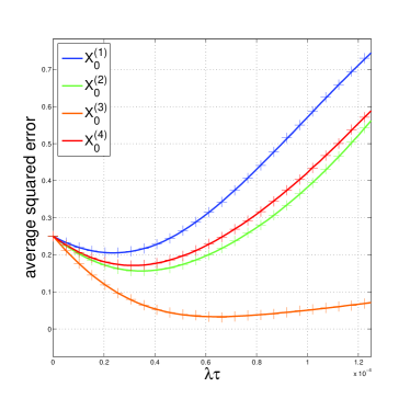
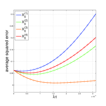
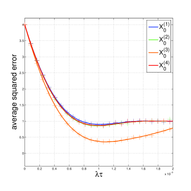
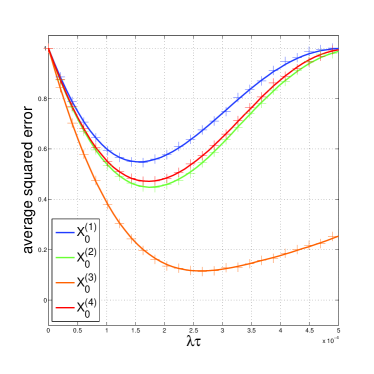
We pause to present some numerical experiments to assess the quality of SURE as an estimate of the risk. We work with four matrices ${\bm{X}}^{0}_{i}$, $i=1,\ldots,4$, of size $200\times 500$. Here, ${\bm{X}}^{0}_{1}$ has full rank; ${\bm{X}}^{0}_{2}$ has rank $100$; ${\bm{X}}^{0}_{3}$ has rank $10$; and ${\bm{X}}^{0}_{4}$ has singular values equal to $\sigma_{i}=\sqrt{200}/(1+\text{e}^{(i-100)/20})$, $i=1,\ldots,200$. Finally, each matrix is normalized so that $\|{\bm{X}}^{0}_{i}\|_{F}=1$, $i=1,\ldots,4$. Next, two methods are used to estimate the risk (1.6) of $\mathrm{SVT}_{\lambda}$ seen as a function of $\lambda$. The first methods uses

$$\hat{R}_{i}(\lambda)=\frac{1}{50}\sum_{j=1}^{50}\|\mathrm{SVT}_{\lambda}({\bm{Y}}_{j}^{(i)})-{\bm{X}}^{0}_{i}\|_{F}^{2},$$

where $\{{\bm{Y}}^{(j)}_{i}\}_{j=1}^{50}$ are independent samples drawn from model (1.1) with ${\bm{X}}^{0}={\bm{X}}^{0}_{i}$. We set this to be the value of reference. The second uses $\textsc{SURE}(\mathrm{SVT}_{\lambda})({\bm{Y}})$, where ${\bm{Y}}$ is drawn from model (1.1) independently from $\{{\bm{Y}}^{(i)}_{j}\}$. Finally, in each case we work with values of the signal-to-noise ratio, defined here as $\text{SNR}=\|{\bm{X}}^{0}\|_{F}/\sqrt{mn}\tau=1/\sqrt{mn}\tau$, and set $\text{SNR}=0.5,1,2$ and $4$. The results are shown in Figure 1, where one can see that SURE remains very close to the true value of the risk, even though it is calculated from a single observation. Matlab code reproducing the figures is available and computing SURE formulas for various spectral estimators is available at http://www-stat.stanford.edu/~candes/SURE_SVT_code.zip.

Figure 1: Comparison of the risk estimate using Monte Carlo (solid line) and SURE (cross) versus $\lambda\times\tau$ for ${\bm{X}}^{0}\in\mathbb{R}^{200\times 500}$ and: (a) $\text{SNR}=0.5$; (b) $\text{SNR}=1$; (c) $\text{SNR}=2$; and (d) $\text{SNR}=4$. The colors indicate the matrices used in each case. As we can see, SURE follows closely the Monte Carlo estimates, even though it requires only one observation to estimate the risk.

In MR applications, observations can take on complex values. Indeed, MRI scanners employ a process known as quadrature detection (two orthogonal phase-sensitive detectors) to observe both the magnitude and phase of rotating magnetization that is induced by radio-frequency (RF) excitation [18]. Quadrature detection both increases SNR and allows for the encoding of motion information like flow. MRI noise, which is Gaussian, is also complex valued. In general, MRI noise can also be assumed iid, noting that inter-channel correlation in parallel MRI data can be removed via Cholesky pre-whitening. Thus, model (1.1) has to be modified as

$${\bm{Y}}={\bm{X}}^{0}+{\bm{W}},\qquad\mathrm{Re}(W_{ij}),\,\mathrm{Im}(W_{ij})\stackrel{{\scriptstyle\text{iid}}}{{\sim}}\mathcal{N}(0,\tau^{2}),$$ (1.9)

where the real and imaginary parts are also independent. In this case, SURE becomes

$$\textsc{SURE}(\mathrm{SVT}_{\lambda})({\bm{Y}})=-2mn\tau^{2}+\sum_{i=1}^{\min(m,n)}\min(\lambda^{2},\sigma_{i}^{2})+2\tau^{2}\mathrm{div}\,(\mathrm{SVT}_{\lambda}({\bm{Y}})).$$

We also provide an expression for the weak divergence in this context, namely,

$$\mathrm{div}\,(\mathrm{SVT}_{\lambda}({\bm{Y}}))=\sum_{i=1}^{\min(m,n)}\left[\mathbb{I}(\sigma_{i}>\lambda)+(2|m-n|+1)\left(1-\frac{\lambda}{\sigma_{i}}\right)_{+}\right]+4\sum_{i\neq j,\,i,j=1}^{\min(m,n)}\frac{\sigma_{i}(\sigma_{i}-\lambda)_{+}}{\sigma_{i}^{2}-\sigma_{j}^{2}},$$ (1.10)

when ${\bm{Y}}$ is simple, and 0 otherwise. This formula can be readily applied to MR data as we shall see in Section 2. The decomposition into real and imaginary parts would suggest that the divergence would be proportional to twice the divergence in the real case. However, this is not the case. The most significant difference is that there is a contribution of the inverse of the singular values even when the matrix is square.

1.3 Extensions

The formulae (1.8)–(1.10) have applications beyond SURE. For instance, the divergence of an estimation procedure arises naturally when trying to estimate the degrees of freedom associated with it. Consider the estimate $\mathrm{SVT}_{\lambda}({\bm{Y}})$ of ${\bm{X}}^{0}$ when the observation ${\bm{Y}}$ comes from an additive error model. The degrees of freedom [11, 32] are defined as

$$\mathrm{df}(\mathrm{SVT}_{\lambda})=\sum_{i=1}^{m}\sum_{j=1}^{n}\mathbf{cov}\left(\mathrm{SVT}_{\lambda}({\bm{Y}})_{ij},Y_{ij}\right).$$

When the observations ${\bm{Y}}$ follow model (1.1), it is possible to write the degrees of freedom as

$$\mathrm{df}(\mathrm{SVT}_{\lambda})=\operatorname{\mathbb{E}}\{\mathrm{div}(\mathrm{SVT}_{\lambda}({\bm{Y}}))\}.$$

Therefore, the expression we provide is also useful to estimate or calculate the degrees of freedom of singular value thresholding.

Finally, although our work focuses on $\mathrm{SVT}$, our methods extend beyond this particular estimator. Consider estimators given by spectral functions. These act on the singular values and take the form

$$f({\bm{Y}})=\sum_{i=1}^{\min(m,n)}f_{i}(\sigma_{i}){\bm{u}}_{i}{\bm{v}}_{i}^{*}:={\bm{U}}f({\bm{\Sigma}}){\bm{V}}^{*},\quad\text{for all }{\bm{Y}}\in\mathbb{R}^{m\times n},$$ (1.11)

where ${\bm{Y}}={\bm{U}}{\bm{\Sigma}}{\bm{V}}^{*}$ is any SVD ($\mathrm{SVT}$ is in this class). Our methods show that these functions admit a SURE formula, given by

$$\textsc{SURE}(f)({\bm{Y}})=-mn\tau^{2}+\|f({\bm{Y}})-{\bm{Y}}\|_{F}^{2}+2\tau^{2}\mathrm{div}\,(f({\bm{Y}})),$$

and that under mild assumptions there exists a closed-form for their divergence:

$$\mathrm{div}\,(f({\bm{X}}))=\sum_{i=1}^{\min(m,n)}\left(f^{\prime}_{i}(\sigma_{i})+|m-n|\frac{f^{\prime}_{i}(\sigma_{i})}{\sigma_{i}}\right)+2\sum_{i\neq j,\,i,j=1}^{\min(m,n)}\frac{\sigma_{i}f_{i}(\sigma_{i})}{\sigma_{i}^{2}-\sigma_{j}^{2}}.$$ (1.12)

This is of interest because such estimators arise naturally in regularized regression problems. For instance, let $J:\mathbb{R}^{m\times n}\mapsto\mathbb{R}$ be a lower semi-continuous, proper convex function of the form

$$J({\bm{X}})=\sum_{i=1}^{\min(m,n)}J_{i}(\sigma_{i}({\bm{X}})),$$

Then, for $\lambda>0$ the estimator

$$f_{\lambda}({\bm{Y}})=\arg\min_{{\bm{X}}\in\mathbb{R}^{m\times n}}\frac{1}{2}\|{\bm{Y}}-{\bm{X}}\|_{F}^{2}+\lambda J({\bm{X}})$$ (1.13)

is spectral. Hence, (1.13) can be used broadly.

1.4 Connections to other works

During the preparation of this manuscript, the conference paper [8] came to our attention and we would like to point out some differences between this work and ours. In [8], the authors propose to recursively estimate the divergence of an estimator given by (1.13). This is done by using proximal splitting algorithms. To this end, they provide an expression for the directional subdifferential of a matrix-valued spectral function. The divergence is then estimated by averaging subdifferentials taken along random directions at each iteration of the proximal algorithm. Our approach is obviously different since we provide closed-form formulas for the divergence that are simple to manipulate and easy to evaluate. This has clear numerical and conceptual advantages. In particular, since we have a closed-form expression for SURE, it becomes easier to understand the risk of a family of estimators. Finally, we also address the case of complex-valued data that seems out of the scope of [8].

1.5 Content

The structure of the paper is as follows. In Section 2 we present applications in MRI illustrating the advantages of choosing the threshold in a disciplined fashion. Section 3 provides precise statements, and a rigorous justification for (1.8) and (1.10). Section 4 deals with the differentiability of spectral functions (1.11), and thus supports Section 3. We conclude with a short discussion of our results, and potential research directions in Section 5.

2 Applications in Magnetic Resonance Imaging (MRI)

SVT is a computationally-straightforward, yet, powerful denoising strategy for MRI applications where spatio-temporal/parameteric behavior is either a priori unknown or else defined accordingly to a complicated nonlinear model that may be numerically challenging to work with. A practical challenge in most rank-based estimation problems in MRI (and inverse problems in general), however, lies in the selection of the regularization or threshold parameter. Defining an automated, disciplined, and consistent methodology for selecting this parameter inherently improves clinical workflow both by accelerating the tuning process through the use of optimization-based, rather than heuristic, search strategies and by freeing the MRI scanner technician so that they can focus on other patient-specific tasks. Moreover, eliminating the human element from the denoising process mitigates inter- and intra-operator variability, and thus raises diagnostic confidence in the denoising results since images are wholly reproducible.

2.1 Noise reduction in cardiac MRI series

Here, we demonstrate a potential use of the SVT unbiased risk estimate for automated and optimized denoising of dynamic cardiac MRI series. Dynamic cardiac imaging is performed either in cine or real-time mode. Cine MRI, the clinical gold-standard for measuring cardiac function/volumetrics [3], produces a movie of roughly 20 cardiac phases over a single cardiac cycle (heart beat). However, by exploiting the semi-periodic nature of cardiac motion, it is actually formed over many heart beats. Cine sampling is gated to a patient’s heart beat, and as each data measurement is captured it is associated with a particular cardiac phase. This process continues until enough data has been collected such that all image frames are complete. Typically, an entire 2D cine cardiac MRI series is acquired within a single breath hold (less than 30 secs).

In real-time cardiac MRI, an image series covering many heart beats is generated. Although the perceived temporal resolution of this series is coarser than that of a cine series, the “temporal footprint” of each frame is actually shorter since it is only comprised of data from one cardiac cycle. Real-time cardiac MRI is of increasing clinical interest for studying transient functional processes such as first-pass myocardial perfusion, where the hemodynamics of an intravenously-injected contrast bolus are visualized. First-pass myocardial perfusion proffers visualization of both damage to heart muscle as well as coronary artery blockage. Typically, a real-time cardiac MRI study will exceed feasible breath-hold time and respiratory motion may be visible.

Simultaneously achieving high spatial resolution and SNR is challenging in both cine and real-time cardiac MRI due to the dynamic nature of the target signal. Signal averaging (NEX $\geq 1$), a standard MRI techniques for noise reduction, is infeasible in real-time imaging and undesirable in cine imaging due to potential misregistration artifacts, since it cannot be executed within a single breath-hold. Real-time acquisitions, which are generally based on gradient recalled echo (GRE) protocols, have inherently low SNR due to their use of very short repetition (TR) and echo times (TE). Cine acquisitions use either standard GRE or balanced steady-state free precession (bSSFP) protocols. When imaging with 1.5 T (Tesla) magnets, bSSFP cine sequences can often yield sufficient SNR. However, unlike many other MRI protocols, SSFP sequences do not trivially gain SNR when moved to higher-field systems ($\geq$ 3.0 T) [26] which is an emerging clinical trend. As magnetic field strength is increased, the RF excitation flip angle used in a bSSFP sequence must be lowered to adhere to RF power deposition (SAR) safety limits. This results in weaker signal excitation which can mitigate gains in bulk magnetization. Poor receiver coil sensitivity at the heart’s medial location and signal loss due to iron overload (hemochromatosis), among other factors, can further reduce SNR in both imaging strategies. Beyond confounding visual radiological evaluation, even moderate noise levels in a cardiac image can also degrade the performance of automated segmentation methods that are used for quantitative cardiac function evaluation. Therefore, effective denoising techniques that preserve the morphological and dynamic profiles of cardiac image series are clinical valuable.

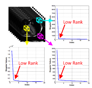
Consider a series of $t$ separate $n\times{n}$ 2D MR images. To utilize SVT to denoise this data, it must first be transformed into a $n^{2}\times{t}$ Casorati matrix, ${\bm{Y}}={\bm{X}}^{0}+{\bm{W}}$. In many MRI scenarios, spatial dimensionality will greatly exceed temporal/parametric dimensionality ($n^{2}\gg t$) and ${\bm{Y}}$ typically is a very thin matrix. Due to limited degrees-of-freedom, even optimally-parameterized SVT may result in temporal/parametric blurring. One solution to this problem is to analyze the image series in a spatial block-wise manner (see Figure 2) rather than globally [36].

Figure 2: Singular values of the Casorati matrices formed from three different $8\times 8\times 19$ block sets extracted from a cine cardiac sequence, including: a static region (cyan); a dynamic region (yellow); and background noise (magenta).

Let ${\bm{R}}_{b}$ be a binary operator that extracts $k^{2}$ rows from a matrix corresponding to a $k\times{k}$ spatial block, specified by index $b$, within each image. Block-wise SVT can be defined as

$$\mathrm{BSVT}_{\lambda}({\bm{Y}})=c^{-1}\sum_{b\in\Omega}{\bm{R}}_{b}^{*}\,\mathrm{SVT}_{\lambda}({\bm{R}}_{b}{\bm{Y}}),$$ (2.1)

where $\Omega$ denotes a set of (potentially overlapping) blocks that uniformly tiles the image domain, i.e., $\sum_{b\in\Omega}{\bm{R}}_{b}^{*}{\bm{R}}_{b}=c{\bm{I}}_{n^{2}\times{n^{2}}}$, $c>0$. In words, (2.1) performs SVT on a family of submatrices of ${\bm{Y}}$ and accumulates a weighted sum of the results. Of course, for $k=n$ and $|\Omega|=1$, (2.1) resorts to standard SVT. The unbiased risk estimator developed in the previous section readily extends for this generalized SVT model. By linearity,

$$\mathrm{div}\,\mathrm{BSVT}_{\lambda}({\bm{Y}})=c^{-1}\sum_{b\in\Omega}\mathrm{div}\,{\bm{R}}_{b}^{*}\,\mathrm{SVT}_{\lambda}({\bm{R}}_{b}{\bm{Y}}).$$ (2.2)

Extending the identity (10) from [2] for matrices then asserts

$$\mathrm{div}\,{\bm{R}}_{b}^{*}\,\mathrm{SVT}_{\lambda}({\bm{R}}_{b}{\bm{Y}})=\sum_{ij}\frac{\partial({\bm{R}}_{b}^{*}\,\mathrm{SVT}_{\lambda}({\bm{R}}_{b}{\bm{Y}}))_{ij}}{\partial Y_{ij}}=\sum_{ij}\frac{\partial\,\mathrm{SVT}_{\lambda}({\bm{R}}_{b}{\bm{Y}})_{ij}}{\partial({\bm{R}}_{b}{\bm{Y}})_{ij}}({\bm{R}}_{b}{\bm{R}}_{b}^{*})_{ii}.$$ (2.3)

Now, observing that ${\bm{R}}_{b}{\bm{R}}_{b}^{*}={\bm{I}}_{k^{2}\times{k^{2}}}$, $\forall{b}\,\in\Omega$, we see that $\mathrm{div}\,{\bm{R}}_{b}^{*}\,\mathrm{SVT}_{\lambda}({\bm{R}}_{b}{\bm{Y}})=\mathrm{div}\,\mathrm{SVT}_{\lambda}({\bm{R}}_{b}{\bm{Y}})$, where the latter term is as in (1.8) for ${\bm{Y}}\in\mathbb{R}^{n^{2}\times{t}}$ or (1.10) for ${\bm{Y}}\in\mathbb{C}^{n^{2}\times{t}}$. Define the mean-squared error of $\mathrm{BSVT}_{\lambda}$ as

$$\text{MSE}(\lambda)=\operatorname{\mathbb{E}}\|{\bm{X}}_{0}-\mathrm{BSVT}_{\lambda}({\bm{Y}})\|_{F}^{2},$$ (2.4)

and the singular value decomposition ${\bm{R}}_{b}{\bm{Y}}={\bm{U}}_{b}{\bm{\Sigma}}_{b}{\bm{V}}_{b}^{*}$. An unbiased estimator of (2.4) is

$$\textsc{SURE}(\mathrm{BSVT}_{\lambda})({\bm{Y}})=-\beta{mn}\tau^{2}+c^{-2}\left\|\sum_{b\in\Omega}{\bm{R}}_{b}^{*}{\bm{U}}_{b}\mathcal{H}_{\lambda}({\bm{\Sigma}}_{b}){\bm{V}}_{b}^{*}\right\|_{F}^{2}+2\tau^{2}c^{-1}\sum_{b\in{\Omega}}\mathrm{div}\,\mathrm{SVT}_{\lambda}({\bm{R}}_{b}{\bm{Y}}),$$ (2.5)

where $\mathcal{H}({\bm{\Sigma}}_{b})_{ij}=\min(\lambda,{\bm{\Sigma}}_{ij})=\mathbb{I}(i=j)\min(\lambda,\sigma_{i})$ and $\sigma_{i}=(\Sigma_{b})_{ii}$. For ${\bm{Y}}\in\mathbb{R}^{n^{2}\times{t}}$, $\beta=1$; otherwise, for ${\bm{Y}}\in\mathbb{C}^{n^{2}\times{t}}$, $\beta=2$.

We now present three MRI examples, one on simulated data and two on real clinical data, and demonstrate the utility of the developed unbiased risk estimators for automatic parameterization of SVT-based denoising.

Example 1: PINCAT Numerical Phantom

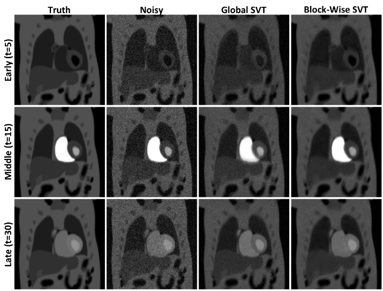
Figure 3: Comparison of MSE-optimized global and block-wise SVT for denoising the complex-valued numerical PINCAT phantom. All images are identically windowed and leveled.

Initial evaluation of SURE for SVT was performed on the physiologically-improved NCAT (PINCAT) numerical phantom [31], which simulates a first-pass myocardial perfusion real-time MRI series. In particularly, the free-breathing model ($n=128$, $t=50$) available in the kt-SLR software package [19] was adapted to include a spatially-smooth and temporally-varying phase field such that the target signal was complex valued. Complex iid  Gaussian noise ($\tau$ = 30) was then added to the image data. Both standard, or global, and block-wise SVT were each executed at 101 values equispaced over $[10^{-1},10^{7}]$. Block-wise SVT was performed with $k=7$ and $\Omega$ comprising one block for each image pixel, under periodic boundary conditions, such that $|\Omega|=n^{2}$.

Figure 4: (a) Plots of MSE and SURE for global and block-wise SVT as a function of threshold value, $\lambda$; the minimizing parameters were used to generate the images in Fig. 3. (b) and (c) show the worst-case error through time of the MSE/SURE-optimized global and block-wise SVT results, respectively.

Figure 3 shows early, middle, and late time frames from the PINCAT series for the noise-free (truth), noisy, and SVT-denoising results. The threshold values used to generate the SVT results were selected as the MSE/SURE-minimizers in Figure 4a. Also observe in Figure 4a that SURE provides a precise estimate of MSE for both the global and block-wise SVT models. The high accuracy exhibited in this case can be attributed to the high dimensionality of the MRI series data. Note that both global and block-wise SVT yield strong noise reduction generally preserve both morphology and contrast. However, block-wise SVT simultaneously demonstrates a greater degree of noise removal and fidelity to ground truth. In particular, note the relative contrast of the various components of the heart in late frame results. The first observation is corroborated by Figure 4a, which shows that block-wise SVT is able to achieve a lower MSE than global SVT. The second observation is corroborated by Figures 4b-c, which show the worst-case absolute error (compared to ground truth) through time for the two SVT setups. Clearly, global SVT exhibits higher residual error than block-wise SVT, particularly in areas of high motion near the myocardium. The difference between these results can be attributed to the matrix anisotropy problem discussed earlier in this section. Thus, SURE can also be used to automatically-determine the block-size setting as well as the threshold value.

Example 2: Cine Cardiac Imaging

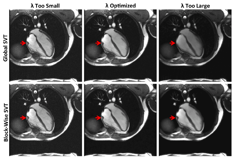
Figure 5: Global and block-wise SVT denoising results for a bSSFP long-axis cine cardiac MRI series. The effect of selecting too high or low a threshold value, as compared to the MSE/SURE optimal value is demonstrated. The red arrow identifies the tricuspid valve of the heart, which exhibit a large degree of motion through the sequence. All images are identically windowed and leveled.

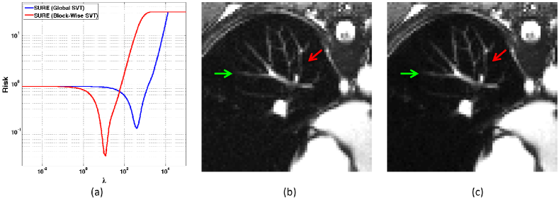
In the second experiment, a bSSFP long-axis cine sequence ($n=192$, $t=19$) acquired at 1.5 T using an phased-array cardiac receiver coil ($\l=8$ channels) was denoised via SVT. The Casorati matrices for individual data channels, which have undergone pre-whitening, are stacked to form a single $ln^{2}\times{t}$ matrix. Assuming that the spatial sensitivity of the receiver channels does not vary substantially through time, the rank of this composite matrix will be equal to that for any individual channel. For visualization purposes, multi-channel denoising results were compressed by calculating the root-sum-of-squares image across the channel dimension. Background noise was determined using a manually-drawn region-of-interest (ROI) to have $\tau$ = 0.67. In this example, block-wise SVT was performed with $k=5$ and used the same block set as in Example 1. The parameter sweep was executed for 101 values equispaced over $[10^{-3},10^{5}]$. In this example, the ground truth is unknown, and thus the MSE cannot be computed to be compared against SURE. However, inspection of Figure 6a reveals that the same qualitative behavior seen for SURE in the numerical phantom example is observed here as well.

Figure 6: (a) SURE for global and block-wise SVT as a function of threshold value, $\lambda$; the minimizing parameters were used to generate the images in Fig. 5. (b) and (c) show enlargements of the pulmonary branching vessels for the SURE-optimized global and block-wise SVT results in Fig. 5, respectively. Red and green arrows highlight improved vessel conspicuity. Both images are windowed and leveled identically.

Figure 5 demonstrates the effect of sub-optimally selecting the threshold value for both global and block-wise SVT. In particular, over- and under-estimates, along with the SURE-optimal values are applied within SVT. For both SVT strategies, under-estimation of $\lambda$ fails to remove noise as expected. Conversely, over-estimation of $\lambda$ leads to spatio-temporal blurring by both strategies albeit in different manners. In global SVT, temporal blurring occurs near areas of high motion like the tricuspid valve of the heart (indicated via the red arrow). However, less active areas like the pulmonary branching vessels, seen just above the heart, are undistorted. Some background noise also remains visible. In the block-wise SVT result, these characteristics are essentially reversed—minimal temporal blurring is induced but there is noticeable spatial blurring and loss of low-contrast static features. Noise is, however, strongly reduced. A compromise between these extremes is made by the SURE-optimized results. As suggested by Figure 6a, block-wise SVT offers stronger noise suppression (see Figures 6b-c) without inducing spatial or temporal blur, the latter which is seen even in the optimized global SVT result. This example highlights the sensitivity of SVT-denoising performance on parameter selection, and the importance of having a disciplined framework for choosing threshold values. Also of note is that, even after empirical pre-whitening, multi-channel MRI noise may not be exactly iid Gaussian. Nonetheless, SURE allows production of extremely reliable results.

Example 3: First-Pass Myocardial Perfusion

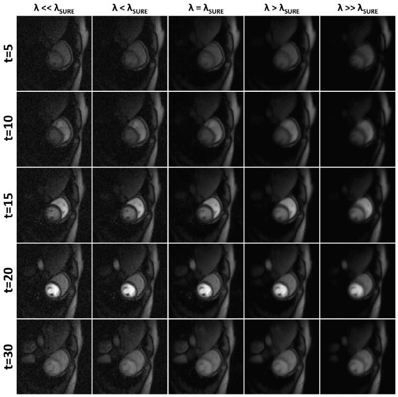
Figure 7: Block-wise SVT denoising results for GRE short-axis first-pass myocardial perfusion sequence. The effect of selecting too high or low a threshold value, as compared to the MSE/SURE optimal value, is demonstrated. All images are identically windowed and leveled.

The third denoising experiment was performed on the single-channel, first-pass myocardial perfusion real-time MRI sequence ($n_{x}=190$, $n_{y}=90$, $t=70$) that is also provided with the kt-SLR software package [19]. To simulate a low-field acquisition (1.0 T), such as with an open or interventional MRI system, complex Gaussian noise was added to the data originally acquired at 3.0 T using a GRE sequence. Following this addition, the noise level was estimated at $\tau=0.105$. Since the duration of this exam exceeded feasible breath-hold time, there is substantial respiratory motion at the end of the series. For this example, only block-wise SVT ($k=6$) denoising was performed, and executed at 101 threshold values equispaced over $[10^{-3},10^{5}]$. As in Example 2, $\Omega$ comprises one block for each image pixel, and only SURE can be computed due to the absence of ground truth.

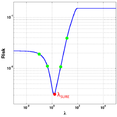
Figure 8: SURE for block-wise SVT as a function of threshold value, $\lambda$; the red dot indicates the optimal threshold value used in Fig. 7, and green dots correspond to the employed under- and over-estimated values.

Mirroring Figure 5, Figure 7 demonstrates the effect of threshold selection on different image frames from the perfusion series. In particular, images showing the transition of contrast from the right to left vertical, as well as later-stage onset of myocardial blush are shown. Of the 101 tested threshold values, 5 threshold settings corresponding to 2 over-estimation, 2 under-estimation, and the SURE-optimal value are depicted (see Figure 8). Under all display settings, temporal contrast dynamics are well preserved; however, threshold setting has a marked effect on noise level, spatial resolution, and contrast. As before, employing SVT with an under-estimated threshold fails to remove noise, as evident in the first two columns of Figure 7. Conversely, employing SVT with an over-estimated threshold will remove noise but also induce both spatial blurring and contrast loss. This is particularly evident in the 4th image row ($t=20$). At high threshold values, the contrast of pulmonary vasculature is diminished, and there is visible blurring of the papillary muscles, which appear as dark spots in the contrast-enhanced left ventricle. Finally, the SVT result obtained with the SURE-optimal threshold represents an ideal balance between these extremes, offering strong noise reduction without degradation of important anatomical features. As suggested by Figure 8, there may only exist a narrow parameter window in which effective denoising can be achieved, and the presented unbiased risk estimators can greatly aid in the identification of these optimal settings.

2.2 Extensions and generalizations

The three examples in the previous subsection demonstrate the utility of the unbiased risk estimation for SVT-based denoising of cardiac MRI series data. Of course, this methodology can also be applied to any other dynamic or parametric MRI series, including those discussed earlier such as functional MRI. Although exhaustive search over a wide range of threshold values was performed for the sake of exposition, the observed unimodality of the risk functional suggests that practical automated parameter selection for SVT denoising could be accelerated using a bisection strategy such as golden section search.

In addition to optimizing over a range of threshold values, unbiased risk estimation can also be used to identify the optimal block-size when using the local SVT model in (2.1). For example, one could imagine performing a sweep of $\lambda$ over a prescribed range of values for a collection of block-size values, and computing the lower envelope of this set of risk measures to investigate best achievable performance as a function of block-size. In addition to simply optimizing a denoising setup, this type of information can be used to guide the development of rank-based reconstruction frameworks for undersampled dynamic and/or parallel MRI.

3 SURE Formulas for Singular Value Thresholding

In [32], Stein gave a formula for an unbiased estimate of the mean-squared error of an estimator obeying a weak differentiability assumption and mild integrability conditions. Before reviewing this, recall that a function $g:\mathbb{R}^{p}\mapsto\mathbb{R}$ is said to be weakly differentiable with respect to the variable $x_{i}$ if there exists $h:\mathbb{R}^{p}\mapsto\mathbb{R}$ such that for all compactly supported and infinitely differentiable functions $\varphi$,

$$\int\varphi(x)h(x)\,dx=-\int\frac{\partial\varphi(x)}{\partial x_{i}}g(x)\,dx.$$

Roughly speaking, the derivatives can fail to exist over regions of Lebesgue measure zero.

Proposition 3.1 ([32, 14]).

Suppose that $Y_{ij}\stackrel{{\scriptstyle\textrm{iid}}}{{\sim}}\mathcal{N}(X_{ij},1)$. Consider an estimator $\hat{{\bm{X}}}$ of the form $\hat{{\bm{X}}}={\bm{Y}}+g({\bm{Y}})$, where $g_{ij}:\mathbb{R}^{m\times n}\mapsto\mathbb{R}$ is weakly differentiable with respect to $Y_{ij}$ and

$$\operatorname{\mathbb{E}}\left\{\left|Y_{ij}g_{ij}({\bm{Y}})\right|+\left|\frac{\partial}{\partial Y_{ij}}g_{ij}({\bm{Y}})\right|\right\}<\infty,$$

for $(i,j)\in\mathcal{I}:=\{1,\ldots,m\}\times\{1,\ldots n\}$. Then

$$\operatorname{\mathbb{E}}\|\hat{{\bm{X}}}-{\bm{X}}\|_{F}^{2}=\operatorname{\mathbb{E}}\bigl{\{}mn+2\mathrm{div}\,(g({\bm{Y}}))+\|g({\bm{Y}})\|_{F}^{2}\bigr{\}}.$$ (3.1)

The rest of this section establishes that $\mathrm{SVT}$ obeys these assumptions whereas the deduction of a closed-form expression for its divergence is deferred to Section 4. To achieve this, we record a simple fact that will allow us to study both the real- and complex-valued cases within the same framework. We identify below $\mathbb{R}^{m\times n}$ with $\mathbb{R}^{mn}$.

Lemma 3.2.

Let $g:\mathbb{R}^{m\times n}\mapsto\mathbb{R}^{m\times n}$ with components $g_{ij}:\mathbb{R}^{m\times n}\mapsto\mathbb{R}$. Assume $g({\bm{0}})={\bm{0}}$. If $g$ is Lipschitz with constant $L>0$, i.e.,

$$\forall\,{\bm{X}},{\bm{Y}}:\quad\|g({\bm{X}})-g({\bm{Y}})\|\leq L\|{\bm{X}}-{\bm{Y}}\|,$$

for some norm in $\mathbb{R}^{m\times n}$, then each $g_{ij}$ is weakly differentiable Lebesgue-a.e. in $\mathbb{R}^{m\times n}$. Furthermore, if ${\bm{Y}}\in\mathbb{R}^{m\times n}$ is distributed as in (1.1), then for all pairs $(i,j)$,

$$\operatorname{\mathbb{E}}\left\{\left|Y_{ij}g_{ij}({\bm{Y}})\right|\right\}<\infty\quad\text{ and }\quad\operatorname{\mathbb{E}}\left\{\left|\frac{\partial}{\partial Y_{ij}}g_{ij}({\bm{Y}})\right|\right\}<\infty.$$

Proof Since all norms are equivalent in finite dimensions, $g$ is also Lipschitz with respect to the Frobenius norm. Hence,

$$\forall\,{\bm{X}},{\bm{Y}}:\quad\|g({\bm{X}})-g({\bm{Y}})\|_{F}\leq L\|{\bm{X}}-{\bm{Y}}\|_{F}\quad\Longrightarrow\quad|g_{ij}({\bm{X}})-g_{ij}({\bm{Y}})|\leq L\|{\bm{X}}-{\bm{Y}}\|_{F},$$ (3.2)

for some constant $L$. By Rademacher’s theorem (see Section 3.1.2 in [12]) each component is differentiable Lebesgue-a.e. in $\mathbb{R}^{m\times n}$. Furthermore, these components are weakly differentiable (see Theorem 1 and 2, Section 6.2, in [12]), and both the derivatives and weak derivatives are Lebesgue-a.e. equal.

Regarding the integrability, since $g({\bm{0}})={\bm{0}}$, (3.2) yields $\|g({\bm{Y}})\|_{F}^{2}\leq L^{2}\|{\bm{Y}}\|_{F}^{2}$ and we deduce

$$\operatorname{\mathbb{E}}\|g({\bm{Y}})\|_{F}^{2}\leq L^{2}\operatorname{\mathbb{E}}\|{\bm{Y}}\|_{F}^{2}=L^{2}(mn+\|{\bm{X}}_{0}\|_{F}^{2})<\infty.$$

Furthermore, the Cauchy-Schwarz inequality gives

$$\operatorname{\mathbb{E}}\{|Y_{ij}g_{ij}({\bm{Y}})|\}\leq\operatorname{\mathbb{E}}\{Y_{ij}^{2}\}^{1/2}\operatorname{\mathbb{E}}\{g_{ij}({\bm{Y}})^{2}\}^{1/2}\leq L\left[(1+X_{0,ij}^{2})(mn+\|{\bm{X}}_{0}\|_{F}^{2})\right]^{1/2}<\infty.$$

Finally, (3.2) asserts that the derivatives of $g_{ij}$—whenever they exist—are bounded by $L$. Hence,

$$\operatorname{\mathbb{E}}\left\{\left|\frac{\partial}{\partial Y_{ij}}g_{ij}({\bm{Y}})\right|\right\}\leq\operatorname{\mathbb{E}}\left\{\left|\frac{\partial}{\partial Y_{ij}}g_{ij}({\bm{Y}})\right|^{2}\right\}^{1/2}\leq L,$$

which concludes the proof.  

For pedagogical reasons, we work with singular value thresholding first, before discussing more general spectral estimators in Section 4. Writing $g({\bm{Y}})=\mathrm{SVT}_{\lambda}({\bm{Y}})-{\bm{Y}}$ then, the conditions become

$$\operatorname{\mathbb{E}}\left\{\left|Y_{ij}g_{ij}({\bm{Y}})\right|+\left|\frac{\partial g_{ij}({\bm{Y}})}{\partial Y_{ij}}\right|\right\}\leq\operatorname{\mathbb{E}}\left\{\left|Y_{ij}\mathrm{SVT}_{\lambda}({\bm{Y}})_{ij}\right|+\left|\frac{\partial}{\partial Y_{ij}}\mathrm{SVT}_{\lambda}({\bm{Y}})_{ij}\right|\right\}+\operatorname{\mathbb{E}}\{Y_{ij}^{2}\}+1,$$

and we only need to study the weak differentiability and integrability of $\mathrm{SVT}$.

3.1 The real case

Lemma 3.3.

The mapping $\mathrm{SVT}_{\lambda}$, $\lambda>0$, obeys the assumptions of Proposition 3.1.

Proof By definition, $\mathrm{SVT}_{\lambda}$ is the proximity function of the nuclear norm. Since the nuclear norm is a convex, proper and lower semi-continuous function, $\mathrm{SVT}_{\lambda}$ is Lipschitz and non-expansive (see Chapter 6, Section 30 in [30]). Applying Lemma 3.2 proves the claim.  

The mapping $\mathrm{SVT}_{\lambda}$ may not be differentiable everywhere. Fortunately, since we are interested in weak differentiability, we can discard sets of Lebesgue measure zero. For instance, model (1.1) guarantees that ${\bm{Y}}$ is simple and has full-rank with probability one. Further, since $\mathrm{SVT}_{\lambda}$ acts by applying soft-thresholding to each singular value, it seems natural that matrices with at least one singular value equal to $\lambda$ will be a cause of concern. Consider then

$$\mathcal{F}:=\{{\bm{X}}\in\mathbb{R}^{m\times n}:\,\text{${\bm{X}}$ is simple, has full rank and no singular value exactly equal to $\lambda$}\}.$$

It is clear that the complement of $\mathcal{F}$ has Lebesgue measure zero. Consequently, we can restrict ourselves to the open set $\mathcal{F}$ to look for a divergence. The result below—a corollary of the general Theorem 4.3—establishes that $\mathrm{SVT}$ is differentiable over $\mathcal{F}$, and thus we have a divergence in the usual sense.

Corollary 3.4.

The mapping $\mathrm{SVT}_{\lambda}$ is differentiable over $\mathcal{F}$ and we have

$$\mathrm{div}\,(\mathrm{SVT}_{\lambda}({\bm{X}}))=\sum_{i=1}^{\min(m,n)}\left[\mathbb{I}\{\sigma_{i}>\lambda\}+|m-n|\left(1-\frac{\lambda}{\sigma_{i}}\right)_{+}\right]+2\sum_{i\neq j,\,i,j=1}^{\min(m,n)}\frac{\sigma_{i}(\sigma_{i}-\lambda)_{+}}{\sigma_{i}^{2}-\sigma_{j}^{2}}.$$ (3.3)

Since $\mathrm{SVT}_{\lambda}$ is of the form (1.11) with

$$f_{i}(\sigma)=(\sigma-\lambda)_{+},\quad f_{i}^{\prime}(\sigma)=\mathbb{I}\{\sigma>\lambda\},$$ (3.4)

for $i=1,\ldots,\min(m,n)$ and $\sigma\neq\lambda$, we see that it is differentiable at the singular value matrix of any element of $\mathcal{F}$. Because the elements of $\mathcal{F}$ are also simple and full-rank, we conclude $\mathrm{SVT}_{\lambda}$ is differentiable over $\mathcal{F}$ by Lemma 4.1. Therefore, the proof of (3.3) is a special case of the general Theorem 4.3 from Section 4.

3.2 The complex case

In the complex case, we need to analyze the conditions for SURE with respect to model (1.9), which can be expressed in vector form as

$$\begin{bmatrix}\mathrm{Re}({\bm{Y}})\\ \mathrm{Im}({\bm{Y}})\end{bmatrix}=\begin{bmatrix}\mathrm{Re}({\bm{X}}_{0})\\ \mathrm{Im}({\bm{X}}_{0})\end{bmatrix}+\begin{bmatrix}\mathrm{Re}({\bm{W}})\\ \mathrm{Im}({\bm{W}})\end{bmatrix}.$$ (3.5)

We thus need to study the existence of the weak partial derivatives

$$\frac{\partial}{\partial\mathrm{Re}(Y_{ij})}\mathrm{Re}(\mathrm{SVT}_{\lambda})_{ij}\qquad\text{and}\qquad\frac{\partial}{\partial\mathrm{Im}(Y_{ij})}\mathrm{Im}(\mathrm{SVT}_{\lambda})_{ij},$$

and whether they satisfy our integrability conditions, as these are the only ones that play a role in the divergence.

Lemma 3.5.

The mappings $\mathrm{SVT}_{\lambda}$, $\mathrm{Re}{(\mathrm{SVT}_{\lambda})}$ and $\mathrm{Im}{(\mathrm{SVT}_{\lambda})}$ obey the assumptions of Proposition 3.1.

Proof As in the real case, $\mathrm{SVT}_{\lambda}$ is the prox-function of the nuclear norm and is thus Lipschitz and non-expansive (see Proposition 2.27 in [1]). Hence, the real and imaginary parts are Lipschitz. Applying Lemma 3.2 to both the real and imaginary components proves the claim.  

For the divergence, we write

$$\mathrm{div}\,(\mathrm{SVT}_{\lambda}({\bm{X}}))=\mathrm{div}_{\mathrm{Re}({\bm{X}})}\,(\mathrm{Re}(\mathrm{SVT}_{\lambda})({\bm{X}}))+\mathrm{div}_{\mathrm{Im}({\bm{X}})}\,(\mathrm{Im}(\mathrm{SVT}_{\lambda})({\bm{X}})).$$ (3.6)

As in the real case, we can discard sets of Lebesgue measure zero. Consider then the analogue of $\mathcal{F}$, whose complement has Lebesgue measure zero.

Corollary 3.6.

The mapping $\mathrm{SVT}_{\lambda}$ is differentiable over $\mathcal{F}$, and we have

$$\mathrm{div}\,(\mathrm{SVT}_{\lambda}({\bm{X}}))=\sum_{i=1}^{\min(m,n)}\left[\mathbb{I}\{\sigma_{i}>\lambda\}+(2|m-n|+1)\left(1-\frac{\lambda}{\sigma_{i}}\right)_{+}\right]+4\sum_{i\neq j,\,i,j=1}^{\min(m,n)}\frac{\sigma_{i}(\sigma_{i}-\lambda)_{+}}{\sigma_{i}^{2}-\sigma_{j}^{2}}.$$ (3.7)

The argument regarding the differentiability of $\mathrm{SVT}_{\lambda}$ applies here as well. The proof of the closed-form expression for the divergence is a special case of the general Theorem 4.5 from Section 4 with $f_{i}$ as in (3.4).

4 Differentiability of Spectral Functions: General SURE Formulas

This section introduces some results concerning the differentiability of spectral functions. To simplify the exposition, we work with $m\times n$ matrices ${\bm{X}}$ with $m\geq n$, as all our arguments apply with minor modifications to ${\bm{X}}^{*}$. Below, $\{{\bm{E}}^{ij}\}_{(i,j)\in\mathcal{I}}$ is the canonical basis of $\mathbb{R}^{n\times m}$, ${\bm{I}}_{n\times n}$ is the $n$-dimensional identity matrix and we set

$${\bm{I}}_{m\times n}=\begin{bmatrix}{\bm{I}}_{n\times n}\\ {\bm{0}}\end{bmatrix}.$$

In the real and complex cases, we make use of the reduced and full SVD. The reduced SVD is written as ${\bm{X}}={\bm{U}}{\bm{\Sigma}}{\bm{V}}^{*}$, where ${\bm{U}}$ is $m\times n$ with orthonormal columns and ${\bm{V}}$ is unitary. In the full SVD, ${\bm{X}}=\tilde{{\bm{U}}}{\bm{\Sigma}}{\bm{V}}^{*}$ where $\tilde{{\bm{U}}}$ is $m\times m$ and extends ${\bm{U}}$ to a unitary matrix. Finally, we recall from Section 1 that a spectral function is of the form $f({\bm{X}})={\bm{U}}f({\bm{\Sigma}}){\bm{V}}^{*}$ with

$$f({\bm{\Sigma}})=\operatorname{diag}(f_{1}(\sigma_{1}),\ldots,f_{n}(\sigma_{n})),$$ (4.1)

where we assume that each $f_{i}:\mathbb{R}_{+}\mapsto\mathbb{R}_{+}$ is differentiable. We note that we can relax the differentiability assumption and only require differentiability in a neighborhood of the spectrum of the matrix under study.

To find a closed-form for the divergence of $f$, we first need to determine whether $f$ is differentiable. Using notation from differential calculus (see [10]), recall that $f$ is differentiable at ${\bm{X}}$ if there exists a linear mapping $\mathrm{d}f_{{\bm{X}}}$, called the differential of $f$ at ${\bm{X}}$, such that for all ${\bm{\Delta}}$,

$$\lim_{{\bm{\Delta}}\rightarrow{\bm{0}}}\frac{\|f({\bm{X}}+{\bm{\Delta}})-f({\bm{X}})-\mathrm{d}f_{{\bm{X}}}[{\bm{\Delta}}]\|_{F}}{\|{\bm{\Delta}}\|_{F}}=0.$$

Differentiation obeys the standard rules of calculus and we have

$$\mathrm{d}f[{\bm{\Delta}}]=\mathrm{d}{\bm{U}}[{\bm{\Delta}}]\,f({\bm{\Sigma}})\,{\bm{V}}^{*}+{\bm{U}}\,\mathrm{d}(f\circ{\bm{\Sigma}})[{\bm{\Delta}}]\,{\bm{V}}^{*}+{\bm{U}}\,f({\bm{\Sigma}})\,\mathrm{d}{\bm{V}}[{\bm{\Delta}}]^{*}.$$ (4.2)

where, to lighten the notation above, we have not indicated the point ${\bm{X}}$ at which the differential is calculated (we shall use subscripts whenever necessary). By the chain rule, $\mathrm{d}(f\circ{\bm{\Sigma}})_{\bm{X}}[{\bm{\Delta}}]=\mathrm{d}f_{\bm{\Sigma}}[\mathrm{d}{\bm{\Sigma}}_{\bm{X}}[{\bm{\Delta}}]]$ so that the differentiability of $f$ depends upon the existence of differentials for ${\bm{U}}$, ${\bm{V}}$ and ${\bm{\Sigma}}$ at ${\bm{X}}$ together with that of $f$ at ${\bm{\Sigma}}$.

Standard analysis arguments immediately establish that the function $f$ is differentiable at ${\bm{\Sigma}}$ whenever ${\bm{\Sigma}}$ is simple, as in this case there is no ambiguity as to which function $f_{i}$ is being applied to the singular values. Furthermore, the differentiability of the SVD of a simple matrix with full-rank is a consequence of Theorem 1 and Theorem 2 in [23] applied to ${\bm{X}}^{*}{\bm{X}}$ and ${\bm{X}}{\bm{X}}^{*}$ (see also [16] and [33]). We summarize these arguments in the following lemma.

Lemma 4.1.

Let ${\bm{X}}={\bm{U}}{\bm{\Sigma}}{\bm{V}}^{*}$ be a simple and full-rank matrix and $f$ be a spectral function.

1. The factors of the SVD are differentiable in a neighborhood of ${\bm{X}}$.

2. If $f$ is differentiable at ${\bm{\Sigma}}$, then it is differentiable at ${\bm{X}}$.

We now focus on determining the divergence of $f$ in closed-form. Since there are differences between the real- and complex-valued cases, we treat them separately.

4.1 The real case

Lemma 4.1 asserts that the SVD is differentiable at any simple matrix ${\bm{X}}$ with full-rank. The following result shows that we can determine the differentials of each factor in closed-form.

Lemma 4.2.

Let ${\bm{X}}$ be simple and full-rank. Then the differentials of ${\bm{U}}$ and ${\bm{V}}$ are given by

$$\mathrm{d}{\bm{U}}[{\bm{\Delta}}]=\tilde{{\bm{U}}}{\bm{\Omega}}_{\tilde{{\bm{U}}}}[{\bm{\Delta}}],\qquad\mathrm{d}{\bm{V}}[{\bm{\Delta}}]={\bm{V}}{\bm{\Omega}}_{\bm{V}}[{\bm{\Delta}}]^{*},$$

where ${\bm{\Omega}}_{\tilde{{\bm{U}}}}$ and ${\bm{\Omega}}_{\bm{V}}$ are given in closed-form (4.8) ($\mathrm{d}{\bm{U}}$ is independent of the choice of $\tilde{{\bm{U}}}$). Finally, $\mathrm{d}{\bm{\Sigma}}$ is given by (4.7).

Proof We follow the same method as in [10], which also appears in [27]. Let ${\bm{X}}\in\mathbb{R}^{m\times n}$ ($m\geq n$). For any matrix ${\bm{\Delta}}\in\mathbb{R}^{m\times n}$, we have

$$\mathrm{d}{\bm{X}}[{\bm{\Delta}}]=\mathrm{d}{\bm{U}}[{\bm{\Delta}}]{\bm{\Sigma}}{\bm{V}}^{*}+{\bm{U}}\mathrm{d}{\bm{\Sigma}}[{\bm{\Delta}}]{\bm{V}}^{*}+{\bm{U}}{\bm{\Sigma}}\mathrm{d}{\bm{V}}[{\bm{\Delta}}]^{*}.$$ (4.3)

Since $\tilde{{\bm{U}}}$ and ${\bm{V}}$ are orthogonal, it follows that

$$\tilde{{\bm{U}}}^{*}\mathrm{d}{\bm{X}}[{\bm{\Delta}}]{\bm{V}}=\tilde{{\bm{U}}}^{*}\mathrm{d}{\bm{U}}[{\bm{\Delta}}]{\bm{\Sigma}}+\tilde{{\bm{U}}}^{*}{\bm{U}}\mathrm{d}{\bm{\Sigma}}[{\bm{\Delta}}]+\tilde{{\bm{U}}}^{*}{\bm{U}}{\bm{\Sigma}}\mathrm{d}{\bm{V}}[{\bm{\Delta}}]^{*}{\bm{V}}.$$

Introduce the matrices

$${\bm{\Omega}}_{\tilde{{\bm{U}}}}[{\bm{\Delta}}]=\tilde{{\bm{U}}}^{*}\mathrm{d}{\bm{U}}[{\bm{\Delta}}]\qquad\text{and}\qquad{\bm{\Omega}}_{\bm{V}}[{\bm{\Delta}}]=\mathrm{d}{\bm{V}}[{\bm{\Delta}}]^{*}{\bm{V}},$$

so that

$$\tilde{{\bm{U}}}^{*}{\bm{\Delta}}{\bm{V}}={\bm{\Omega}}_{\tilde{{\bm{U}}}}[{\bm{\Delta}}]{\bm{\Sigma}}+{\bm{I}}_{m\times n}\mathrm{d}{\bm{\Sigma}}[{\bm{\Delta}}]+{\bm{I}}_{m\times n}{\bm{\Sigma}}{\bm{\Omega}}_{\bm{V}}[{\bm{\Delta}}],$$ (4.4)

where we used the fact that $\mathrm{d}{\bm{X}}$ is the identity, whence $\mathrm{d}{\bm{X}}[{\bm{\Delta}}]={\bm{\Delta}}$. Moreover,

$${\bm{0}}=\mathrm{d}{\bm{I}}_{n\times n}({\bm{\Delta}})={\bm{V}}^{*}\mathrm{d}{\bm{V}}[{\bm{\Delta}}]+\mathrm{d}{\bm{V}}[{\bm{\Delta}}]^{*}{\bm{V}}\quad\Longrightarrow\quad{\bm{V}}^{*}\mathrm{d}{\bm{V}}[{\bm{\Delta}}]=-\mathrm{d}{\bm{V}}[{\bm{\Delta}}]^{*}{\bm{V}},$$

which says that ${\bm{\Omega}}_{\bm{V}}[{\bm{\Delta}}]$ is anti-symmetric. Similarly,

$${\bm{0}}=\mathrm{d}{\bm{I}}_{n\times n}({\bm{\Delta}})={\bm{U}}^{*}\mathrm{d}{\bm{U}}[{\bm{\Delta}}]+\mathrm{d}{\bm{U}}[{\bm{\Delta}}]^{*}{\bm{U}}\quad\Longrightarrow\quad{\bm{U}}^{*}\mathrm{d}{\bm{U}}[{\bm{\Delta}}]=-\mathrm{d}{\bm{U}}[{\bm{\Delta}}]^{*}{\bm{U}},$$

and thus the upper $n\times n$ block of ${\bm{\Omega}}_{\tilde{{\bm{U}}}}[{\bm{\Delta}}]$ is also anti-symmetric. This fact and the skew-symmetry of ${\bm{\Omega}}_{\bm{V}}[{\bm{\Delta}}]$ yield the relations

$$\Omega_{\tilde{{\bm{U}}},ii}[{\bm{\Delta}}] = 0,\qquad i=1,\ldots,n,$$

$$\Omega_{{\bm{V}},ii}[{\bm{\Delta}}] = 0,\qquad i=1,\ldots,n,$$

$$(\tilde{{\bm{U}}}^{*}{\bm{\Delta}}{\bm{V}})_{ij} = \Omega_{\tilde{{\bm{U}}},ij}[{\bm{\Delta}}]\sigma_{j}+\sigma_{i}\Omega_{{\bm{V}},ij}[{\bm{\Delta}}],\qquad i\neq j,\quad i,j=1,\ldots,n,$$ (4.5)

$$-(\tilde{{\bm{U}}}^{*}{\bm{\Delta}}{\bm{V}})_{ji} = \Omega_{\tilde{{\bm{U}}},ij}[{\bm{\Delta}}]\sigma_{i}+\sigma_{j}\Omega_{{\bm{V}},ij}[{\bm{\Delta}}],\qquad i\neq j,\quad i,j=1,\ldots,n,$$ (4.6)

and

$$\mathrm{d}\sigma_{i}[{\bm{\Delta}}]=(\tilde{{\bm{U}}}^{*}{\bm{\Delta}}{\bm{V}})_{ii},\qquad i=1,\ldots,n.$$ (4.7)

In particular, (4.5) and (4.6) can be summarized in the system of linear equations

$$\begin{bmatrix}\sigma_{j}&\sigma_{i}\\ \sigma_{i}&\sigma_{j}\end{bmatrix}\begin{bmatrix}\Omega_{\tilde{{\bm{U}}},ij}[{\bm{\Delta}}]\\ \Omega_{{\bm{V}},ij}[{\bm{\Delta}}]\end{bmatrix}=\begin{bmatrix}(\tilde{{\bm{U}}}^{*}{\bm{\Delta}}{\bm{V}})_{ij}\\ -(\tilde{{\bm{U}}}^{*}{\bm{\Delta}}{\bm{V}})_{ji}\end{bmatrix},\qquad i\neq j,\quad i,j=1,\ldots,n.$$

Since ${\bm{X}}$ is simple, the coefficient matrix is invertible, and thus

$$\begin{bmatrix}\Omega_{\tilde{{\bm{U}}},ij}[{\bm{\Delta}}]\\ \Omega_{{\bm{V}},ij}[{\bm{\Delta}}]\end{bmatrix}=-\frac{1}{\sigma_{i}^{2}-\sigma_{j}^{2}}\begin{bmatrix}\sigma_{j}&\sigma_{i}\\ -\sigma_{i}&-\sigma_{j}\end{bmatrix}\begin{bmatrix}(\tilde{{\bm{U}}}^{*}{\bm{\Delta}}{\bm{V}})_{ij}\\ (\tilde{{\bm{U}}}^{*}{\bm{\Delta}}{\bm{V}})_{ji}\end{bmatrix},\qquad i\neq j,\quad i,j=1,\ldots,n.$$ (4.8)

These relations determine both $\mathrm{d}{\bm{\Sigma}}[{\bm{\Delta}}]$, ${\bm{\Omega}}_{\bm{V}}[{\bm{\Delta}}]$ and the upper $n\times n$ block of ${\bm{\Omega}}_{\tilde{{\bm{U}}}}[{\bm{\Delta}}]$ completely. The lower $(m-n)\times n$ block of ${\bm{\Omega}}_{\tilde{{\bm{U}}}}[{\bm{\Delta}}]$ is determined from (4.4), as

$$(\tilde{{\bm{U}}}^{*}{\bm{\Delta}}{\bm{V}})_{ij}=\Omega_{\tilde{{\bm{U}}},ij}[{\bm{\Delta}}]\sigma_{j},\qquad i=n+1,\ldots,m,\quad j=1,\ldots,n.$$ (4.9)

Since ${\bm{X}}$ has full-rank, this completely determines ${\bm{\Omega}}_{\tilde{{\bm{U}}}}[{\bm{\Delta}}]$. We conclude that (i) $\mathrm{d}{\bm{\Sigma}}[{\bm{\Delta}}]$, ${\bm{\Omega}}_{{\bm{V}}}[{\bm{\Delta}}]$ and ${\bm{\Omega}}_{{\bm{U}}}[{\bm{\Delta}}]$ are uniquely characterized by the SVD of ${\bm{X}}$, and (ii) they act linearly on ${\bm{\Delta}}$. Furthermore, the differentials obey (4.3). We now prove that $\mathrm{d}{\bm{U}}[{\bm{\Delta}}]$ is independent of the choice of $\tilde{{\bm{U}}}$. Decompose ${\bm{\Omega}}_{\tilde{{\bm{U}}}}[{\bm{\Delta}}]$ and $\tilde{{\bm{U}}}$ as

$${\bm{\Omega}}_{\tilde{{\bm{U}}}}[{\bm{\Delta}}]=\begin{bmatrix}{\bm{\Omega}}_{{\bm{U}}}[{\bm{\Delta}}]\\ {\bm{\Omega}}_{{\bm{Q}}}[{\bm{\Delta}}]\end{bmatrix}\qquad\text{and}\qquad\tilde{{\bm{U}}}=\begin{bmatrix}{\bm{U}}&{\bm{Q}}\end{bmatrix},$$

where ${\bm{\Omega}}_{{\bm{U}}}[{\bm{\Delta}}]$ denotes the upper $n\times n$ block of ${\bm{\Omega}}_{\tilde{{\bm{U}}}}[{\bm{\Delta}}]$ (which depends only on ${\bm{U}}$ by (4.8)) and ${\bm{\Omega}}_{{\bm{Q}}}[{\bm{\Delta}}]$ denotes the lower $(m-n)\times n$ block of ${\bm{\Omega}}_{\tilde{{\bm{U}}}}[{\bm{\Delta}}]$ (which by (4.9) equals ${\bm{Q}}^{*}{\bm{\Delta}}{\bm{V}}{\bm{\Sigma}}^{-1}$). Then

$$\mathrm{d}{\bm{U}}[{\bm{\Delta}}]=\tilde{{\bm{U}}}{\bm{\Omega}}_{\tilde{{\bm{U}}}}[{\bm{\Delta}}]={\bm{U}}{\bm{\Omega}}_{{\bm{U}}}[{\bm{\Delta}}]+{\bm{Q}}{\bm{\Omega}}_{{\bm{Q}}}[{\bm{\Delta}}]={\bm{U}}{\bm{\Omega}}_{{\bm{U}}}[{\bm{\Delta}}]+({\bm{Q}}{\bm{Q}}^{*}){\bm{\Delta}}{\bm{V}}{\bm{\Sigma}}^{-1},$$

which is well defined since the orthogonal projector ${\bm{Q}}{\bm{Q}}^{*}$ is independent of the choice of ${\bm{Q}}$.  

Since Lemma 4.2 provides a closed-form expression for the differentials, computing the value of the divergence is now a matter of calculus.

Theorem 4.3.

Let $f$ be a matrix-valued spectral function and suppose ${\bm{X}}\in\mathbb{R}^{m\times n}$ is simple and has full-rank. Then

$$\mathrm{div}\,(f({\bm{X}}))=\sum_{i=1}^{\min(m,n)}\left(f^{\prime}_{i}(\sigma_{i})+|m-n|\frac{f^{\prime}_{i}(\sigma_{i})}{\sigma_{i}}\right)+2\sum_{i\neq j,\,i,j=1}^{\min(m,n)}\frac{\sigma_{i}f_{i}(\sigma_{i})}{\sigma_{i}^{2}-\sigma_{j}^{2}}.$$ (4.10)

Proof Assume $m\geq n$ without loss of generality. Let $\{\tilde{{\bm{u}}}_{i}\}_{i=1}^{m}$ and $\{{\bm{v}}_{i}\}_{i=1}^{n}$ denote the columns of $\tilde{{\bm{U}}}$ and ${\bm{V}}$, and set

$${\bm{\Delta}}^{ij}=\tilde{{\bm{u}}}_{i}{\bm{v}}_{j}^{*},\qquad(i,j)\in\mathcal{I}.$$

Then $\{{\bm{\Delta}}^{ij}\}_{(i,j)\in\mathcal{I}}$ is an orthonormal basis for $\mathbb{R}^{m\times n}$ and, furthermore, $\tilde{{\bm{U}}}^{*}{\bm{\Delta}}^{ij}{\bm{V}}={\bm{E}}^{ij}$. Since $\{{\bm{\Delta}}^{ij}\}_{(i,j)\in\mathcal{I}}$ is an orthonormal basis,

$$\mathrm{div}\,(f({\bm{X}}))=\sum_{(i,j)\in\mathcal{I}}\left\langle{\bm{\Delta}}^{ij},\mathrm{d}f[{\bm{\Delta}}^{ij}]\right\rangle.$$ (4.11)

Note that (4.2) yields

$$\mathrm{d}f[{\bm{\Delta}}^{ij}]=\tilde{{\bm{U}}}^{*}({\bm{\Omega}}_{\tilde{{\bm{U}}}}[{\bm{\Delta}}^{ij}]f({\bm{\Sigma}})+{\bm{I}}_{m\times n}\mathrm{d}(f\circ{\bm{\Sigma}})[{\bm{\Delta}}^{ij}]+{\bm{I}}_{m\times n}f({\bm{\Sigma}}){\bm{\Omega}}_{\bm{V}}[{\bm{\Delta}}^{ij}]){\bm{V}}^{*}.$$

Next, from (4.7) we obtain

$$\mathrm{d}\sigma_{k}[{\bm{\Delta}}^{ij}]=\delta_{ki}\delta_{kj},\qquad(i,j)\in\mathcal{I},\quad k=1,\ldots,n.$$

By the same arguments, from (4.8) we obtain

$$\begin{bmatrix}\Omega_{\tilde{{\bm{U}}},kl}[{\bm{\Delta}}^{ij}]\\ \Omega_{{\bm{V}},kl}[{\bm{\Delta}}^{ij}]\end{bmatrix}=-\frac{1}{\sigma_{k}^{2}-\sigma_{l}^{2}}\begin{bmatrix}\sigma_{l}&\sigma_{k}\\ -\sigma_{k}&-\sigma_{l}\end{bmatrix}\begin{bmatrix}\delta_{ik}\delta_{jl}\\ \delta_{il}\delta_{jk}\end{bmatrix},\qquad(i,j)\in\mathcal{I},\quad k,l=1,\ldots,n,\quad k\neq l,$$

and from (4.9),

$$\Omega_{\tilde{{\bm{U}}},kl}[{\bm{\Delta}}^{ij}]=\frac{\delta_{ik}\delta_{jl}}{\sigma_{l}},\qquad(i,j)\in\mathcal{I},\quad k=n+1,\ldots,m,\quad l=1,\ldots,n.$$

Now follow (4.11) and decompose the divergence as

$$\mathrm{div}\,(f({\bm{X}})) = \sum_{(i,j)\in\mathcal{I}}\left\langle{\bm{E}}^{ij},{\bm{\Omega}}_{\tilde{{\bm{U}}}}[{\bm{\Delta}}^{ij}]f({\bm{\Sigma}})+{\bm{I}}_{m\times n}\mathrm{d}(f\circ{\bm{\Sigma}})[{\bm{\Delta}}^{ij}]+{\bm{I}}_{m\times n}f({\bm{\Sigma}}){\bm{\Omega}}_{\bm{V}}[{\bm{\Delta}}^{ij}]\right\rangle$$

$$= S^{\tilde{{\bm{U}}}}+S^{{\bm{\Sigma}}}+S^{{\bm{V}}}.$$

We see that $S^{{\bm{V}}}$ is equal to

$$S^{{\bm{V}}}=\sum_{i\neq j,\,i,j=1}^{n}f_{ij}({\bm{\Sigma}})\Omega_{{\bm{V}},ij}[{\bm{\Delta}}^{ij}]=\sum_{i\neq j,\,i,j=1}^{n}\frac{f_{i}(\sigma_{i})}{\sigma_{i}^{2}-\sigma_{j}^{2}}(\sigma_{i}\delta_{ii}\delta_{jj}+\sigma_{j}\delta_{ij}\delta_{ji})=\sum_{i\neq j,\,i,j=1}^{n}\frac{\sigma_{i}f_{i}(\sigma_{i})}{\sigma_{i}^{2}-\sigma_{j}^{2}},$$

whereas

$$S^{{\bm{\Sigma}}}=\sum_{i,j=1}^{n}\mathrm{d}f_{ij}[\mathrm{d}\Sigma_{ij}[{\bm{\Delta}}^{ij}]]=\sum_{i,j=1}^{n}\delta_{ij}f_{i}^{\prime}(\sigma_{i})=\sum_{i=1}^{n}f_{i}^{\prime}(\sigma_{i}).$$

Finally, $S^{\tilde{{\bm{U}}}}$ decomposes as

$$S^{\tilde{{\bm{U}}}}=\sum_{i,j=1}^{n}\left\langle{\bm{E}}^{ij},{\bm{\Omega}}_{\tilde{{\bm{U}}}}[{\bm{\Delta}}^{ij}]f({\bm{\Sigma}})\right\rangle+\sum_{i=n+1}^{m}\sum_{j=1}^{n}\left\langle{\bm{E}}^{ij},{\bm{\Omega}}_{\tilde{{\bm{U}}}}[{\bm{\Delta}}^{ij}]f({\bm{\Sigma}})\right\rangle.$$

Using (4.8), the first term is equal to

$$\sum_{i,j=1}^{n}\left\langle{\bm{E}}^{ij},{\bm{\Omega}}_{\tilde{{\bm{U}}}}[{\bm{\Delta}}^{ij}]f({\bm{\Sigma}})\right\rangle=-\sum_{i\neq j,\,i,j=1}^{n}\frac{f_{j}(\sigma_{j})}{\sigma_{i}^{2}-\sigma_{j}^{2}}(\sigma_{j}\delta_{ii}\delta_{jj}+\sigma_{i}\delta_{ij}\delta_{ji})=\sum_{i\neq j,\,i,j=1}^{n}\frac{\sigma_{i}f_{i}(\sigma_{i})}{\sigma_{i}^{2}-\sigma_{j}^{2}},$$

while it follows from (4.9) that the second equals

$$\sum_{i=n+1}^{m}\sum_{j=1}^{n}\left\langle{\bm{E}}^{ij},{\bm{\Omega}}_{\tilde{{\bm{U}}}}[{\bm{\Delta}}^{ij}]f({\bm{\Sigma}})\right\rangle=\sum_{i=1}^{m-n}\sum_{j=1}^{n}\left\langle{\bm{E}}^{ij},{\bm{E}}^{ij}{\bm{\Sigma}}^{-1}f({\bm{\Sigma}})\right\rangle=(m-n)\sum_{i=1}^{n}\frac{f_{i}(\sigma_{i})}{\sigma_{i}}.$$

Since $n=\min(m,n)$, we conclude that

$$\mathrm{div}\,(f({\bm{X}}))=S^{\tilde{{\bm{U}}}}+S^{{\bm{\Sigma}}}+S^{{\bm{V}}}=\sum_{i=1}^{\min(m,n)}\left(f^{\prime}_{i}(\sigma_{i})+|m-n|\frac{f^{\prime}_{i}(\sigma_{i})}{\sigma_{i}}\right)+2\sum_{i\neq j,\,i,j=1}^{\min(m,n)}\frac{\sigma_{i}f_{i}(\sigma_{i})}{\sigma_{i}^{2}-\sigma_{j}^{2}}.$$

 

4.2 The complex case

Since the singular values are not analytic functions of the entries, we can only consider the derivatives of $f$ as a function of the real and imaginary parts of the entries of ${\bm{X}}$. Therefore, we identify $\mathbb{C}^{m\times n}$ with $\mathbb{R}^{m\times n}\times\mathbb{R}^{m\times n}$ and $f$ with a complex-valued function of $2mn$ variables. This has the particular consequence that the differential $\text{d}f$ at ${\bm{X}}\in\mathbb{C}^{m\times n}$—whenever it exists—obeys

$$\mathrm{d}f_{\bm{X}}[{\bm{\Delta}}]=\mathrm{d}f_{\bm{X}}[\mathrm{Re}({\bm{\Delta}})]+\mathrm{d}f_{\bm{X}}[\imath\mathrm{Im}({\bm{\Delta}})],$$

for all ${\bm{\Delta}}\in\mathbb{C}^{m\times n}$; here, $\imath$ is the imaginary unit. The differential seen as a function with domain $\mathbb{R}^{m\times n}\times\mathbb{R}^{m\times n}$ is of course linear. Lemma 4.2 may be adapted to the complex setting with minor modifications.

Lemma 4.4.

Let ${\bm{X}}$ be simple and full-rank. Then the differentials of ${\bm{U}}$ and ${\bm{V}}$ are given by

$$\mathrm{d}{\bm{U}}[{\bm{\Delta}}]=\tilde{{\bm{U}}}{\bm{\Omega}}_{\tilde{{\bm{U}}}}[{\bm{\Delta}}],\qquad\mathrm{d}{\bm{V}}[{\bm{\Delta}}]={\bm{V}}{\bm{\Omega}}_{\bm{V}}[{\bm{\Delta}}]^{*},$$

where ${\bm{\Omega}}_{\tilde{{\bm{U}}}}$ and ${\bm{\Omega}}_{\bm{V}}$ are given in closed-form (4.15) ($\mathrm{d}{\bm{U}}$ is independent of the choice of $\tilde{{\bm{U}}}$). Further, $\mathrm{d}{\bm{\Sigma}}$ is given by (4.13). For completeness, ${\bm{\Omega}}_{\tilde{{\bm{U}}}},{\bm{\Omega}}_{\bm{V}}:\mathbb{C}^{m\times n}\mapsto\mathbb{C}^{m\times n}$ while $\mathrm{d}{\bm{\Sigma}}:\mathbb{C}^{m\times n}\mapsto\mathbb{R}^{m\times n}$.

Proof Following the same steps as in the proof of Lemma 4.2, let ${\bm{X}}\in\mathbb{C}^{m\times n}$ ($m\geq n$). We see that (4.4) becomes

$$\tilde{{\bm{U}}}^{*}{\bm{\Delta}}{\bm{V}}={\bm{\Omega}}_{\tilde{{\bm{U}}}}[{\bm{\Delta}}]{\bm{\Sigma}}+{\bm{I}}_{m\times n}\mathrm{d}{\bm{\Sigma}}[{\bm{\Delta}}]+{\bm{I}}_{m\times n}{\bm{\Sigma}}{\bm{\Omega}}_{\bm{V}}[{\bm{\Delta}}],$$ (4.12)

where ${\bm{\Omega}}_{\bm{V}}$ and the upper $n\times n$ block of ${\bm{\Omega}}_{\tilde{{\bm{U}}}}$ are now skew-Hermitian. Since these matrices have purely imaginary entries on the diagonal,

$$\mathrm{d}\sigma_{i}[{\bm{\Delta}}]=\mathrm{Re}\{(\tilde{{\bm{U}}}^{*}{\bm{\Delta}}{\bm{V}})_{ii}\}=\frac{(\tilde{{\bm{U}}}^{*}{\bm{\Delta}}{\bm{V}})_{ii}+\overline{(\tilde{{\bm{U}}}^{*}{\bm{\Delta}}{\bm{V}})_{ii}}}{2},\qquad i=1,\ldots,n,$$ (4.13)

and

$$\Omega_{\tilde{{\bm{U}}},ii}[{\bm{\Delta}}]\sigma_{i}+\Omega_{{\bm{V}},ii}[{\bm{\Delta}}]\sigma_{i}=\mathrm{Im}\{(\tilde{{\bm{U}}}^{*}{\bm{\Delta}}{\bm{V}})_{ii}\}\imath=\frac{(\tilde{{\bm{U}}}^{*}{\bm{\Delta}}{\bm{V}})_{ii}-\overline{(\tilde{{\bm{U}}}^{*}{\bm{\Delta}}{\bm{V}})_{ii}}}{2},\qquad i=1,\ldots,n.$$ (4.14)

Furthermore, it is not hard to see that the system (4.8) becomes

$$\begin{bmatrix}\Omega_{\tilde{{\bm{U}}},ij}[{\bm{\Delta}}]\\ \Omega_{{\bm{V}},ij}[{\bm{\Delta}}]\end{bmatrix}=-\frac{1}{\sigma_{i}^{2}-\sigma_{j}^{2}}\begin{bmatrix}\sigma_{j}&\sigma_{i}\\ -\sigma_{i}&-\sigma_{j}\end{bmatrix}\begin{bmatrix}({\bm{U}}^{*}{\bm{\Delta}}{\bm{V}})_{ij}\\ \overline{({\bm{U}}^{*}{\bm{\Delta}}{\bm{V}})_{ji}}\end{bmatrix},\qquad i\neq j,\quad i,j=1,\ldots,n,$$ (4.15)

and the expression equivalent to (4.9) is

$$(\tilde{{\bm{U}}}^{T}{\bm{\Delta}}{\bm{V}})_{ij}=\Omega_{\tilde{{\bm{U}}},ij}[{\bm{\Delta}}]\sigma_{j},\qquad i=n+1,\ldots,m,\quad j=1,\ldots,n.$$ (4.16)

As in the real case, this shows $\mathrm{d}{\bm{\Sigma}}[{\bm{\Delta}}]$, ${\bm{\Omega}}_{{\bm{V}}}[{\bm{\Delta}}]$ and ${\bm{\Omega}}_{{\bm{U}}}[{\bm{\Delta}}]$ act linearly on ${\bm{\Delta}}$, and that they are uniquely characterized by the SVD of ${\bm{X}}$. Furthermore, the same argument allows us to show that the differential of ${\bm{U}}$ is independent of the choice of $\tilde{{\bm{U}}}$, concluding the proof.  

As in the real case, we restrict attention to a simple and full-rank ${\bm{X}}\in\mathbb{C}^{m\times n}$. We need to determine two terms for the divergence as discussed in Section 3.2. Now if $\{{\bm{\Delta}}^{ij}\}_{(i,j)\in\mathcal{I}}$ is an orthonormal basis for $\mathbb{R}^{m\times n}$, then $\{\imath{\bm{\Delta}}^{ij}\}_{(i,j)\in\mathcal{I}}$ is an orthonormal basis for $\imath\mathbb{R}^{m\times n}$. With the divergence as in (3.6),

$$\mathrm{div}\,(f({\bm{X}})) = \sum_{(i,j)\in\mathcal{I}}\mathrm{Re}(\left\langle{\bm{\Delta}}^{ij},\mathrm{d}f[{\bm{\Delta}}^{ij}]\right\rangle)+\sum_{(i,j)\in\mathcal{I}}\mathrm{Im}(\left\langle{\bm{\Delta}}^{ij},\mathrm{d}f[\imath{\bm{\Delta}}^{ij}]\right\rangle)$$

$$= \mathrm{Re}\left(\sum_{(i,j)\in\mathcal{I}}\left\langle{\bm{\Delta}}^{ij},\mathrm{d}f[{\bm{\Delta}}^{ij}]-\imath\mathrm{d}f[\imath{\bm{\Delta}}^{ij}]\right\rangle\right).$$

The analogue of Theorem 4.3 is this:

Theorem 4.5.

Let $f$ be a matrix-valued spectral function and suppose ${\bm{X}}\in\mathbb{C}^{m\times n}$ is simple and has full-rank. Then

$$\mathrm{div}\,(f({\bm{X}}))=\sum_{i=1}^{\min(m,n)}\left(f_{i}^{\prime}(\sigma_{i})+(2|m-n|+1)\frac{f_{i}(\sigma_{i})}{\sigma_{i}}\right)+4\sum_{i\neq j,\,i,j=1}^{\min(m,n)}\frac{\sigma_{i}f_{i}(\sigma_{i})}{\sigma_{i}^{2}-\sigma_{j}^{2}}.$$ (4.17)

Proof Since ${\bm{X}}$ is simple and has full-rank, Lemma 4.4 holds, and

$$\mathrm{d}f[{\bm{E}}^{ij}]-\imath\mathrm{d}f[{\bm{E}}^{ij}]=\tilde{{\bm{U}}}\left[({\bm{\Omega}}_{\tilde{{\bm{U}}}}[{\bm{E}}^{ij}]-\imath{\bm{\Omega}}_{\tilde{{\bm{U}}}}[\imath{\bm{E}}^{ij}])f({\bm{\Sigma}})+{\bm{I}}_{m\times n}f({\bm{\Sigma}})({\bm{\Omega}}_{\bm{V}}[{\bm{E}}^{ij}]-\imath{\bm{\Omega}}_{\bm{V}}[\imath{\bm{E}}^{ij}])\right]{\bm{V}}^{*}\\ +\tilde{{\bm{U}}}{\bm{I}}_{m\times n}\mathrm{d}f_{{\bm{\Sigma}}}[\mathrm{d}{\bm{\Sigma}}[{\bm{E}}^{ij}]-\imath\mathrm{d}{\bm{\Sigma}}[\imath{\bm{E}}^{ij}]]{\bm{V}}^{*}.$$ (4.18)

Put ${\bm{L}}^{ij}=\tilde{{\bm{U}}}^{*}{\bm{E}}^{ij}{\bm{V}}$ for $(i,j)\in\mathcal{I}$ for short. From (4.13), we get

$$\mathrm{d}\sigma_{i}[{\bm{E}}^{ij}]-\imath\mathrm{d}\sigma_{i}[\imath{\bm{E}}^{ij}]=L_{kk}^{ij}$$

for $(i,j)\in\mathcal{I}$ and $k=1,\ldots,n$. By the same arguments, (4.15) gives

$$\begin{bmatrix}\Omega_{\tilde{{\bm{U}}},kl}[{\bm{E}}^{ij}]-\imath\Omega_{\tilde{{\bm{U}}},kl}[\imath{\bm{E}}^{ij}]\\ \Omega_{{\bm{V}},kl}[{\bm{E}}^{ij}]-\imath\Omega_{{\bm{V}},kl}[{\bm{E}}^{ij}]\end{bmatrix}=-\frac{1}{\sigma_{k}^{2}-\sigma_{l}^{2}}\begin{bmatrix}\sigma_{l}&\sigma_{k}\\ -\sigma_{k}&-\sigma_{l}\end{bmatrix}\begin{bmatrix}2L^{ij}_{kl}\\ 0\end{bmatrix},$$

for $(i,j)\in\mathcal{I}$, $k,l=1,\ldots,n$, and $k\neq l$. Next, (4.16) gives

$$\Omega_{\tilde{{\bm{U}}},kl}[{\bm{E}}^{ij}]=2\frac{L^{ij}_{kl}}{\sigma_{l}},$$

for $(i,j)\in\mathcal{I}$, $k=n+1,\ldots,m$, and $l=1,\ldots,n$. Finally, (4.14) implies

$${\bm{\Omega}}_{\tilde{{\bm{U}}},kk}[{\bm{E}}^{ij}]+\Omega_{{\bm{V}},kk}[{\bm{E}}^{ij}]-\imath(\Omega_{\tilde{{\bm{U}}},kk}[\imath{\bm{E}}^{ij}]+\Omega_{{\bm{V}},kk}[\imath{\bm{E}}^{ij}])=\frac{L^{ij}_{kk}}{\sigma_{k}},$$

for $k=1,\ldots,n$. Now, set

$$S^{\tilde{{\bm{U}}}} = \sum_{(i,j)\in\mathcal{I}}\left\langle{\bm{L}}^{ij},({\bm{\Omega}}_{\tilde{{\bm{U}}}}[{\bm{E}}^{ij}]-\imath{\bm{\Omega}}_{\tilde{{\bm{U}}}}[\imath{\bm{E}}^{ij}])f({\bm{\Sigma}})\right\rangle,$$

$$S^{{\bm{\Sigma}}} = \sum_{(i,j)\in\mathcal{I}}\left\langle{\bm{L}}^{ij},{\bm{I}}_{m\times n}f({\bm{\Sigma}})({\bm{\Omega}}_{\bm{V}}[{\bm{E}}^{ij}]-\imath{\bm{\Omega}}_{\bm{V}}[\imath{\bm{E}}^{ij}])\right\rangle,$$

$$S^{{\bm{V}}} = \sum_{(i,j)\in\mathcal{I}}\left\langle{\bm{L}}^{ij},{\bm{I}}_{m\times n}\mathrm{d}f_{{\bm{\Sigma}}}[\mathrm{d}{\bm{\Sigma}}[{\bm{E}}^{ij}]-\imath\mathrm{d}{\bm{\Sigma}}[\imath{\bm{E}}^{ij}]]\right\rangle.$$

Then it is clear that

$$S^{{\bm{V}}} = \sum_{(i,j)\in\mathcal{I}}\sum_{k\neq l,\,k,l=1}^{n}\frac{2f_{k}(\sigma_{k})\sigma_{k}|L^{ij}_{kl}|^{2}}{\sigma_{k}^{2}-\sigma_{l}^{2}}+\sum_{k=1}^{n}f_{k}(\sigma_{k})\sum_{(i,j)\in\mathcal{I}}\overline{L^{ij}_{kk}}({\bm{\Omega}}_{{\bm{V}},kk}[{\bm{E}}^{ij}]-\imath{\bm{\Omega}}_{{\bm{V}},kk}[\imath{\bm{E}}^{ij}])$$

$$= 2\sum_{k\neq l,\,k,l=1}^{n}\frac{f_{k}(\sigma_{k})\sigma_{k}}{\sigma_{k}^{2}-\sigma_{l}^{2}}+\sum_{k=1}^{n}f_{k}(\sigma_{k})\sum_{(i,j)\in\mathcal{I}}\overline{L^{ij}_{kk}}({\bm{\Omega}}_{{\bm{V}},kk}[{\bm{E}}^{ij}]-\imath{\bm{\Omega}}_{{\bm{V}},kk}[\imath{\bm{E}}^{ij}]),$$

and

$$S^{{\bm{\Sigma}}}=\sum_{(i,j)\in\mathcal{I}}\sum_{k=1}^{n}f_{k}^{\prime}(\sigma_{k})|L_{kk}^{ij}|^{2}=\sum_{k=1}^{n}f_{k}^{\prime}(\sigma_{k}).$$

Finally,

$$S^{\tilde{{\bm{U}}}} =-\sum_{(i,j)\in\mathcal{I}}\sum_{k\neq l,\,k,l=1}^{n}\frac{2f_{l}(\sigma_{l})\sigma_{l}|L_{kl}^{ij}|^{2}}{\sigma_{k}^{2}-\sigma_{l}^{2}}+\sum_{k=1}^{n}f_{k}(\sigma_{k})\sum_{(i,j)\in\mathcal{I}}\overline{L^{ij}_{kk}}({\bm{\Omega}}_{\tilde{{\bm{U}}},kk}[{\bm{E}}^{ij}]-\imath{\bm{\Omega}}_{\tilde{{\bm{U}}},kk}[\imath{\bm{E}}^{ij}])$$

$$\qquad\qquad+\sum_{(i,j)\in\mathcal{I}}\sum_{k=n+1}^{m}\sum_{l=1}^{n}2\frac{f_{l}(\sigma_{l})|L^{ij}_{kl}|^{2}}{\sigma_{l}}$$

$$=2\sum_{k\neq l,\,k,l=1}^{n}\frac{f_{k}(\sigma_{k})\sigma_{k}}{\sigma_{k}^{2}-\sigma_{l}^{2}}+2(m-n)\sum_{k=1}^{n}\frac{f_{k}(\sigma_{k})}{\sigma_{k}}+\sum_{k=1}^{n}f_{k}(\sigma_{k})\sum_{(i,j)\in\mathcal{I}}\overline{L^{ij}_{kk}}({\bm{\Omega}}_{\tilde{{\bm{U}}},kk}[{\bm{E}}^{ij}]-\imath{\bm{\Omega}}_{\tilde{{\bm{U}}},kk}[\imath{\bm{E}}^{ij}]).$$

Since

$$\sum_{(i,j)\in\mathcal{I}}\overline{L^{ij}_{kk}}\left({\bm{\Omega}}_{\tilde{{\bm{U}}},kk}[{\bm{E}}^{ij}]-\imath{\bm{\Omega}}_{\tilde{{\bm{U}}},kk}[\imath{\bm{E}}^{ij}]+{\bm{\Omega}}_{{\bm{V}},kk}[{\bm{E}}^{ij}]-\imath{\bm{\Omega}}_{{\bm{V}},kk}[\imath{\bm{E}}^{ij}]\right)=\sum_{(i,j)\in\mathcal{I}}\frac{|L^{ij}_{kk}|^{2}}{\sigma_{k}}=\frac{1}{\sigma_{k}},$$

we conclude

$$\mathrm{div}\,(f({\bm{X}})) = \mathrm{Re}\left(S^{\tilde{{\bm{U}}}}+S^{{\bm{\Sigma}}}+S^{{\bm{V}}}\right)$$

$$= \sum_{i=1}^{\min(m,n)}\left(f_{i}^{\prime}(\sigma_{i})+(2|m-n|+1)\frac{f_{i}(\sigma_{i})}{\sigma_{i}}\right)+4\sum_{i\neq j,\,i,j=1}^{\min(m,n)}\frac{\sigma_{i}f_{i}(\sigma_{i})}{\sigma_{i}^{2}-\sigma_{j}^{2}},$$

where we used $n=\min(m,n)$.  

4.3 An extension to all matrix arguments

Theorems 4.3 and 4.5 provide the divergence of a matrix-valued spectral function in closed-form for simple, full-rank arguments. Here, we indicate that these formulas have a continuous extension to all matrices. Before continuing, we introduce some notation. For a given ${\bm{X}}$, we denote as $\kappa\leq n$ the number of distinct singular values while $s_{i}$ and $d_{i}$, $i=1,\ldots,\kappa$, denote the $i$-th distinct singular value and its multiplicity.

As previously discussed, when ${\bm{\Sigma}}$ is simple there is no ambiguity as to which $f_{i}$ is being applied to a singular value. However, when ${\bm{\Sigma}}$ is not simple, the ambiguities make $f$ nondifferentiable unless $f_{i}\equiv f$ for $i=1,\ldots,n$.

Theorem 4.6.

Let $f$ be a matrix-valued spectral function, with $f_{i}\equiv f$ for $i=1,\ldots,n$, and $f(0)=0$. Then the divergence extends by continuity to any ${\bm{X}}\in\mathbb{R}^{m\times n}$, and is given by

$$\mathrm{div}\,(f({\bm{X}})) = \sum_{i:\,s_{i}>0}\left[\left(d_{i}+{d_{i}\choose 2}\right)f^{\prime}(s_{i})+\left(|m-n|d_{i}+{d_{i}\choose 2}\right)\frac{f(s_{i})}{s_{i}}\right]$$ (4.19)

$$+ \sum_{i:\,s_{i}=0}\left[(|m-n|+1)d_{i}+2{d_{i}\choose 2}\right]f^{\prime}(0)+2\sum_{i\neq j,\,i,j=1}^{\kappa}d_{i}d_{j}\frac{s_{i}f(s_{i})}{s_{i}^{2}-s_{j}^{2}},$$

and to any ${\bm{X}}\in\mathbb{C}^{m\times n}$,

$$\mathrm{div}\,(f({\bm{X}})) = \sum_{i:\,s_{i}>0}\left[\left(d_{i}+2{d_{i}\choose 2}\right)f^{\prime}(s_{i})+\left((2|m-n|+1)d_{i}+2{d_{i}\choose 2}\right)\frac{f(s_{i})}{s_{i}}\right]$$ (4.20)

$$+ \sum_{i:\,s_{i}=0}\left[2(|m-n|+1)d_{i}+4{d_{i}\choose 2}\right]f^{\prime}(0)+4\sum_{i\neq j,\,i,j=1}^{\kappa}d_{i}d_{j}\frac{s_{i}f(s_{i})}{s_{i}^{2}-s_{j}^{2}}.$$

Proof We only prove (4.19) as the same arguments apply to (4.20). The key idea involves non-tangential limits defined below. Suppose we have a sequence $\{{\bm{X}}_{k}\}$ of full-rank matrices with ${\bm{X}}_{k}\rightarrow{\bm{X}}$ as $k\rightarrow\infty$; we establish that the limit $\mathrm{div}(f({\bm{X}}_{k}))$ is independent of the sequence. Since (4.10) depends only on the singular values of ${\bm{X}}_{k}$, we can focus on the sequence of singular values. Let $\{\sigma_{i}\}_{i=1}^{n}$ be the singular values of ${\bm{X}}$, and let $\{\sigma_{i}^{k}\}_{i=1}^{n}$ be those of ${\bm{X}}_{k}$. We have

$$\mathrm{div}\,(f({\bm{X}}_{k}))=\sum_{i=1}^{\min(m,n)}\left(f^{\prime}(\sigma_{i}^{k})+|m-n|\frac{f(\sigma_{i}^{k})}{\sigma_{i}^{k}}\right)+2\sum_{i\neq j,\,i,j=1}^{\min(m,n)}\frac{\sigma_{i}^{k}f(\sigma_{i}^{k})}{(\sigma_{i}^{k})^{2}-(\sigma_{j}^{k})^{2}}.$$

The first terms are easy to analyze. In fact,

$$\lim_{k\rightarrow\infty}f^{\prime}(\sigma_{i}^{k})=f^{\prime}(\sigma_{i})\quad\text{and}\quad\lim_{k\rightarrow\infty}\frac{f(\sigma_{i}^{k})}{\sigma_{i}^{k}}=\begin{cases}\frac{f(\sigma_{i})}{\sigma_{i}},&\text{if $\sigma_{i}>0$,}\\ f^{\prime}(0),&\text{if $\sigma_{i}=0$.}\end{cases}$$

The remaining term can be decomposed as

$$\sum_{i\neq j,\,i,j=1}^{\min(m,n)}\frac{\sigma_{i}^{k}f(\sigma_{i}^{k})}{(\sigma_{i}^{k})^{2}-(\sigma_{j}^{k})^{2}}=\left[\sum_{i\neq j,\,\sigma_{i}=\sigma_{j}}^{\min(m,n)}+\sum_{i\neq j,\,\sigma_{i}\neq\sigma_{j}}^{\min(m,n)}\right]\frac{\sigma_{i}^{k}f(\sigma_{i}^{k})}{(\sigma_{i}^{k})^{2}-(\sigma_{j}^{k})^{2}}:=I_{0}+I_{1}.$$ (4.21)

We now formalize the notion of non-tangential limit. Consider a pair $(i,j)$ with $i\neq j$ and $\sigma_{i}=\sigma_{j}:=\sigma$, and define

$$\delta^{k}_{i}=\sigma_{i}^{k}-\sigma,\quad\delta^{k}_{j}=\sigma_{j}^{k}-\sigma\quad\text{and}\quad\rho^{k}_{ij}=\delta^{k}_{j}/\delta^{k}_{i}.$$

We say that ${\bm{X}}_{k}$ approaches ${\bm{X}}$ non-tangentially if there exists a constant $c_{ij}>0$ such that $|\rho^{k}_{ij}-1|>c_{ij}$. Roughly speaking, the matrices ${\bm{X}}_{k}$ approach ${\bm{X}}$ fast enough, so that they remain simple, and have full-rank. We have

$$\frac{\sigma_{i}^{k}f(\sigma_{i}^{k})-\sigma_{j}^{k}f(\sigma_{j}^{k})}{(\sigma_{i}^{k})^{2}-(\sigma_{j}^{k})^{2}} = \frac{\sigma}{2\sigma+\delta^{k}_{i}+\delta^{k}_{j}}\left(\frac{f(\sigma+\delta_{i}^{k})-f(\sigma+\delta_{j}^{k})}{\delta_{i}^{k}-\delta_{j}^{k}}\right)$$

$$+ \frac{1}{2\sigma+\delta^{k}_{i}+\delta^{k}_{j}}\left(\frac{1}{1-\rho_{ij}^{k}}f(\sigma+\delta_{i}^{k})-\frac{\rho^{k}_{ij}}{1-\rho_{ij}^{k}}f(\sigma+\delta_{j}^{k})\right).$$

We distinguish two cases. If $\sigma>0$, we see that

$$\lim_{k\rightarrow\infty}\frac{\sigma_{i}^{k}f(\sigma_{i}^{k})-\sigma_{j}^{k}f(\sigma_{j}^{k})}{(\sigma_{i}^{k})^{2}-(\sigma_{j}^{k})^{2}}=\frac{1}{2}f^{\prime}(\sigma)+\frac{1}{2}\frac{f(\sigma)}{\sigma}$$

whereas when $\sigma=0$ we obtain

$$\lim_{k\rightarrow\infty}\frac{\sigma_{i}^{k}f(\sigma_{i}^{k})-\sigma_{j}^{k}f(\sigma_{j}^{k})}{(\sigma_{i}^{k})^{2}-(\sigma_{j}^{k})^{2}}=f^{\prime}(0)$$

and, therefore,

$$I_{0}=\sum_{i:\,s_{i}=0}{d_{i}\choose 2}f^{\prime}(0)+\frac{1}{2}\sum_{i:\,s_{i}>0}{d_{i}\choose 2}\left(f^{\prime}(s_{i})+\frac{f(s_{i})}{s_{i}}\right).$$

The second sum $I_{1}$ in (4.21) is easier to analyze, as it can be seen that

$$\lim_{k\rightarrow\infty}\sum_{i\neq j,\,\sigma_{i}\neq\sigma_{j}}^{\min(m,n)}\frac{\sigma_{i}^{k}f(\sigma_{i}^{k})}{(\sigma_{i}^{k})^{2}-(\sigma_{j}^{k})^{2}}=\sum_{i\neq j,\,i,j=1}^{\kappa}d_{i}d_{j}\frac{s_{i}f(s_{i})}{s_{i}^{2}-s_{j}^{2}},$$

concluding the proof.  

5 Discussion

Beyond MRI, SVT denoising also has potential application for medical imaging modalities outside of MRI. For example, in perfusion X-ray computed tomography (CT) studies, where some anatomical region (e.g., the kidneys) is repeatedly scanned to visualize hemodynamics, X-ray tube energy is routinely lowered to limit the ionizing radiation dose delivered to the patient. However, this can result in a substantial increase of image noise. Recent works (e.g., [4]) have shown that retrospective denoising of low-dose CT data can often yield diagnostic information comparable to full-dose images. It may be possible to adapt SVT, and the proposed risk estimators, for the CT dose reduction problem as well.

Following the successful application of compressive sensing theory [7, 9] for accelerated MRI (e.g.,  [20, 35]), the use of low-rank constraints for undersampled MRI reconstruction is also of increasing interest. For the dynamic and parametric acquisition scenarios described above, the generalization from denoising to undersampled reconstruction is straightforward in light of recent developments on the topic of matrix completion [6, 29]. To date, low-rank reconstruction methods have been deployed for accelerated cardiac imaging [13, 19, 36] and dynamic contrast-enhanced MRI (DCE-MRI) of the breast [13]. More recently, it has been demonstrated that reconstructing accelerated parallel MRI data under low-rank constraints [21, 37] can obviate the need for expensive and potentially error-prone patient-specific calibration procedures as well as facilitate previously impractical acquisition strategies. As with the denoising application, parameter selection is an outstanding challenge in undersampled reconstruction problems. Unlike the denoising problem, only incomplete noisy data is available and Stein’s method is not directly applicable. Recently, for undersampled MRI reconstruction, Ramani et al. [28] demonstrated that Stein’s method can be used to generate an unbiased risk estimator for the predicted MSE of $\ell_{1}$-minimization reconstructions, and that this can be used for automated parameter optimization. An interesting future direction of research will lie in determining if the models developed in this work facilitate development of a similar framework for the low-rank matrix recovery problem.

Acknowledgements

E. C. is partially supported by AFOSR under grant FA9550-09-1-0643, by ONR under grant N00014-09-1-0258 and by a gift from the Broadcom Foundation. C. S-L. is partially supported by a Fulbright-CONICYT Scholarship and by the Simons Foundation. J. D. T. and the Mayo Clinic Center for Advanced Imaging Research are partially supported by National Institute of Health grant RR018898. E. C. would like to thank Rahul Mazumder for fruitful discussions about this project.

References

• [1] H. H. Bauschke and P. L. Combettes. Convex analysis and monotone operator theory in Hilbert spaces. CMS Books in Mathematics. Springer, 2011.
• [2] T. Blu and F. Luisier. The SURE-LET approach to image denoising. IEEE Transactions on Image Processing, 16(11):2778–2786, 2007.
• [3] J. Bogaert, S. Dymarkowski, and A. M. Taylor. Clinical cardiac MRI. Medical Radiology: Diagnostic Imaging. Springer, 2005.
• [4] A. Borsdorf, R. Raupach, T. Flohr, and J. Hornegger. Wavelet based noise reduction in CT-images using correlation analysis. IEEE Transactions on Medical Imaging, 27(12):1695–1703, 2008.
• [5] J. A. Cadzow. Signal enhancement - a composite property mapping algorithm. IEEE Transactions on Acoustics, Speech and Signal Processing, 36(1):49–62, 1988.
• [6] E. J. Candès and B. Recht. Exact matrix completion via convex optimization. Foundations of Computational Mathematics, 9(6):717–772, 2009.
• [7] E. J. Candès, J. Romberg, and T. Tao. Robust uncertainty principles: exact signal reconstruction from highly incomplete frequency information. IEEE Transactions on Information Theory, 52(2):489–509, 2006.
• [8] C.-A. Deledalle, S. Vaiter, G. Peyré, J. Fadili, and C. Dossal. Risk estimation for matrix recovery with spectral regularization. arXiv:1205.1482v1, May 2012.
• [9] D.L. Donoho. Compressed sensing. IEEE Transactions on Information Theory, 52(4):1289–1306, 2006.
• [10] A. Edelman. Handouts for 18.325: Matrix jacobians without wedge products, 2005.
• [11] B. Efron, T. Hastie, I. Johnstone, and R. Tibshirani. Least angle regression. Annals of Statistics, 32:407–499, 2004.
• [12] L. C. Evans and R. F. Gariepy. Measure theory and fine properties of functions. Boca Raton, FL: CRC Press, 1992.
• [13] J. Haldar and Z.-P. Liang. spatiotemporal imaging with partially separable functions: a matrix recovery approach. In Proceedings of the IEEE International Symposium on Biomedical Imaging (ISBI), pages 716–719, 2010.
• [14] I. Johnstone. Gaussian estimation: Sequence and wavelet models. Springer Texts in Statistics. Manuscript, December 2007.
• [15] F. Lam, S. D. Babacan, J. P. Haldar, N. Schuff, and Z.-P. Liang. Denoising diffusion-weighted MR magnitude image sequences using low rank and edge constraints. In Proceedings of the IEEE International Symposium on Biomedical Imaging (ISBI), pages 1401–1404, 2012.
• [16] A. Lewis and H. Sendov. Twice differentiable spectral functions. SIAM Journal on Matrix Analysis and Applications, 23(2):368–386, 2001.
• [17] Z.-P. Liang. Spatiotemporal imaging with partially separable functions. In Proceedings of the IEEE International Symposium on Biomedical Imaging (ISBI), pages 988–991, 2007.
• [18] Z.-P. Liang and P. C. Lauterbur. Principles of Magnetic Resonance Imaging: A Signal Processing Perspective. Biomedical Engineering. IEEE, 2000.
• [19] S. G. Lingala, Y. Hu, E. DiBella, and M. Jacob. Accelerated dynamic MRI exploiting sparsity and low-rank structure: kt-SLR. IEEE Transactions on Medical Imaging, 30(5):1042–1054, 2011.
• [20] M. Lustig, D. L. Donoho, and J. M. Pauly. Sparse MRI: The application of compressed sensing for rapid mr imaging. Magnetic Resonance in Medicine, 58(6):1182–1195, 2007.
• [21] M. Lustig, M. Elad, and J. M. Pauly. Calibrationless parallel imaging reconstruction by structured low-rank matrix completion. In Proceedings of the 18th Annual Meeting of the International Society for Magnetic Resonance in Medicine (ISMRM), page 2870, 2010.
• [22] Bydder M. and Du J. Noise reduction in multiple-echo data sets using singular value decomposition. Magnetic Resonance Imaging, 24(7):849–856, 2006.
• [23] J. R. Magnus. On differentiating eigenvalues and eigenvectors. Econometric Theory, 1(2):pp. 179–191, 1985.
• [24] J. V. Manjon, P. Coupe, L. Concha, A. Buades, L. Collins, and M. Robles. DWI denoising using overcomplete local PCA decomposition. In Proceedings of the 20th Annual Meeting of the International Society for Magnetic Resonance in Medicine (ISMRM), page 3580, 2012.
• [25] H. M. Nguyen, X. Peng, M. N. Do, and Z.-P. Liang. Spatiotemporal denoising of MR spectroscopic imaging data by low-rank approximations. In Proceedings of the IEEE International Symposium on Biomedical Imaging (ISBI), pages 857–860, 2011.
• [26] J. N. Oshinski, J. G. Delfino, P. Sharma, A. M. Gharib, and Pettigrew R. I. Cardiovascular magnetic resonance at 3.0 T: current state of the art. Journal of Cardiac Magnetic Resonance, 12(1):55, 2010.
• [27] T. Papadopoulo and M. I. A. Lourakis. Estimating the jacobian of the singular value decomposition: Theory and applications. In Proceedings of the European Conference on Computer Vision, ECCV’00, pages 554–570. Springer, 2000.
• [28] S. Ramani, Z. Liu, J. Rosen, J.-F. Nielsen, and J. A. Fessler. Regularization parameter selection for nonlinear iterative image restoration and MRI reconstruction using GCV and SURE-based methods. IEEE Transactions on Image Processing, 21(8):3659–3672, 2012.
• [29] B. Recht, M. Fazel, and P. A. Parrilo. Guaranteed minimum rank solutions to linear matrix equations via nuclear norm minimization. SIAM Review, 52(3):471–501, 2010.
• [30] R. T. Rockafellar. Convex analysis. Princeton landmarks in mathematics. Princeton, NJ: Princeton University Press, 1997.
• [31] B. Shariff and Y. Bresler. Physiologically improved NCAT Phantom (PINCAT) enables in-silico study of the effects of beat-to-beat variability on cardiac MR. In Proceedings of the 15th Annual Meeting of the International Society for Magnetic Resonance in Medicine (ISMRM), page 3418, 2007.
• [32] C. M. Stein. Estimation of the mean of a multivariate normal distribution. The Annals of Statistics, 9(6):pp. 1135–1151, 1981.
• [33] D. Sun and J. Sun. Nonsmooth matrix valued functions defined by singular values. http://www.math.nus.edu.sg/ matsundf/SS3.pdf, December 2002.
• [34] C. G. Thomas, R. A. Harshman, and R. S. Menon. Noise reduction in BOLD-based fMRI using component analysis. NeuroImage, 17(3):1521–1537, 2002.
• [35] J. D. Trzasko and A. Manduca. Highly undersampled magnetic resonance image reconstruction via homotopic 0subscript0\ell_{0} -minimization. IEEE Transactions on Medical Imaging, 28(1):106–121, 2009.
• [36] J. D. Trzasko and A. Manduca. Local versus global low-rank promotion in dynamic MRI series reconstruction. In Proceedings of the 19th Annual Meeting of the International Society for Magnetic Resonance in Medicine (ISMRM), page 4371, 2011.
• [37] J. D. Trzasko and A. Manduca. CLEAR: Calibration-free parallel imaging using locally low-rank encouraging reconstruction. In Proceedings of the 20th Annual Meeting of the International Society for Magnetic Resonance in Medicine (ISMRM), page 517, 2012.