An Online Manifold Learning Approach for Model Reduction of Dynamical Systems

Abstract

This article discusses a newly developed online manifold learning method, subspace iteration using reduced models (SIRM), for the dimensionality reduction of dynamical systems. This method may be viewed as subspace iteration combined with a model reduction procedure. Specifically, starting with a test solution, the method solves a reduced model to obtain a more precise solution, and it repeats this process until sufficient accuracy is achieved. The reduced model is obtained by projecting the full model onto a subspace that is spanned by the dominant modes of an extended data ensemble. The extended data ensemble in this article contains not only the state vectors of some snapshots of the approximate solution from the previous iteration but also the associated tangent vectors. Therefore, the proposed manifold learning method takes advantage of the information of the original dynamical system to reduce the dynamics. Moreover, the learning procedure is computed in the online stage, as opposed to being computed offline, which is used in many projection-based model reduction techniques that require prior calculations or experiments. After providing an error bound of the classical POD-Galerkin method in terms of the projection error and the initial condition error, we prove that the sequence of approximate solutions converge to the actual solution of the original system as long as the vector field of the full model is locally Lipschitz on an open set that contains the solution trajectory. Good accuracy of the proposed method has been demonstrated in two numerical examples, from a linear advection-diffusion equation to a nonlinear Burgers equation. In order to save computational cost, the SIRM method is extended to a local model reduction approach by partitioning the entire time domain into several subintervals and obtaining a series of local reduced models of much lower dimensionality. The accuracy and efficiency of the local SIRM are shown through the numerical simulation of the Navier–Stokes equation in a lid-driven cavity flow problem.

1 Introduction

The simulation, control, design, and analysis of the methods and algorithms for many large-scale dynamical systems are often computationally intensive and require massive computing resources if at all possible. The idea of model reduction is to provide an efficient computational prototyping tool to replace a high-order system of differential equations with a system of a substantially lower dimension, whereby only the most dominant properties of the full system are preserved. During the past several decades, several model reduction methods have been studied, such as Krylov subspace methods [4], balanced truncation [16, 23, 12], and proper orthogonal decomposition (POD) [16, 13]. More techniques can be found in  [3] and [2]. These model reduction methods are usually based on offline computations to build the empirical eigenfunctions of the reduced model before the computation of the reduced state variables. Most of the time these offline computations are as complex as the original simulation. For these reasons, an efficient reduced model with high fidelity based on online manifold learning is preferable. However, much less effort has been expended in the field of model reduction via online manifold learning. In  [22], an incremental algorithm involving adaptive periods was proposed. During these adaptive periods the incremental computation is restarted until a quality criterion is satisfied. In [14] and [17] state vectors from previous time steps are extracted to span a linear subspace in order to construct the reduced model for the next step. In  [18] dynamic iteration using reduced order models (DIRM) combines the idea of the waveform relaxation technique and model reduction, which simulates each subsystem that is connected to model reduced versions of the other subsystems.

A new framework of iterative manifold learning, subspace iteration using reduced models (SIRM), is proposed in this article for the reduced modeling of high-order nonlinear dynamical systems. Similar to the well-known Picard iteration for solving ODEs, a trial solution is set at the very beginning. Using POD, a set of updated empirical eigenfunctions are constructed in each iteration by extracting dominant modes from an extended data ensemble; then, a more accurate solution is obtained by solving the reduced equation in a new subspace spanned by these empirical eigenfunctions. The extended data ensemble contains not only the state vectors of some snapshots of the trajectory in the previous iteration but also the associated tangent vectors. Therefore, the manifold learning process essentially takes advantage of the information from the original dynamical system. Both analytical results and numerical simulations indicate that a sequence of functions asymptotically converges to the solution of the full system. Moreover, the aforementioned method can be used to test (and improve) the accuracy of a trial solution of other techniques. A posterior error estimation can be estimated by the difference between the trial solution and a more precise solution obtained by SIRM.

The remainder of this article is organized as follows. Since algorithms in this article fall in the category of projection methods, the classic POD-Galerkin method and its ability to minimize truncation error are briefly reviewed in section 2. After presenting the SIRM algorithm in section 3, we provide convergence analysis, complexity analysis, and two numerical examples. Then SIRM is combined with the time domain partition in section 4, and a local SIRM method is proposed to decrease redundant dimensions. The performance of this technique is evaluated in a lid-driven cavity flow problem. Finally, conclusions are offered.

2 Background of Model Reduction

Let $J=[0,T]$ denote the time domain, $x:J\to\mathbb{R}^{n}$ denote the state variable, and $f:J\times\mathbb{R}^{n}\to\mathbb{R}^{n}$ denote the discretized vector field. A dynamical system in $\mathbb{R}^{n}$ can be described by an initial value problem

(1) $$\dot{x}=f(t,x);\ \ \ \ \ x(0)=x_{0}.$$

By definition, $x(t)$ is a flow that gives an orbit in $\mathbb{R}^{n}$ as $t$ varies over $J$ for a fixed $x_{0}$. The orbit contains a sequence of states (or state vectors) that follow from $x_{0}$.

2.1 Galerkin projection

For a $k$-dimensional linear subspace $S$ in $\mathbb{R}^{n}$, there exists an $n\times k$ orthonormal matrix $\Phi=[\phi_{1},...,\phi_{k}]$, the columns of which form a complete basis of $S$. The orthonormality of the column matrix requires that $\Phi^{T}\Phi=I$, where $I$ is an identity matrix. Any state $x\in\mathbb{R}^{n}$ can be projected onto $S$ by a linear projection. The projected state is given by $\Phi^{T}x\in\mathbb{R}^{k}$ in the subspace coordinate system, where superscript $T$ denotes the matrix transpose. Let $P:=\Phi\Phi^{T}$ denote the projection matrix in $\mathbb{R}^{n}$. Then, the same projection in the original coordinate system is represented by $\tilde{x}(t):=Px(t)\in\mathbb{R}^{n}$.

Let $\Phi^{T}f(t,\Phi z)$ denote a reduced-order vector field formed by Galerkin projection. The corresponding reduced model for $z(t)\in\mathbb{R}^{k}$ is

(2) $$\dot{z}=\Phi^{T}f(t,\Phi z);\ \ \ \ \ z_{0}=\Phi^{T}x_{0}.$$

An approximate solution in the original coordinate system $\hat{x}(t)=\Phi z(t)\in\mathbb{R}^{n}$ is equivalent to the solution of the following ODE:

(3) $$\dot{\hat{x}}=Pf(t,\hat{x});\ \ \ \ \ \hat{x}_{0}=Px_{0}.$$

It is well-known that the existence and uniqueness of a solution for system (1) can be proved by the Picard iteration.

Lemma 1 (Picard–Lindelöf existence and uniqueness [15]).

Suppose there is a closed ball of radius $b$ around a point $x_{0}\in\mathbb{R}^{n}$ such that $f:J_{a}\times B_{b}(x_{0})\to\mathbb{R}^{n}$ is a uniformly Lipschitz function of $x\in B_{b}(x_{0})$ with constant $K$, and a continuous function of $t$ on $J_{a}=[0,a]$. Then the initial value problem (1) has a unique solution $x(t)\in B_{b}(x_{0})$ for $t\in J_{a}$, provided that $a=b/M$, where

(4) $$M=\mathop{\max}\limits_{(t,x)\in J_{a}\times B_{b}(x_{0})}\left\|{f(t,x)}\right\|.$$

Similarly, a reduced model formed by Galerkin projection also has a unique local solution if the original vector field is Lipschitz. Moreover, the existence and uniqueness of solutions do not depend on the projection operator.

Lemma 2 (local existence and uniqueness of reduced models).

With $a$, $J_{a}$, $b$, $B_{b}(x_{0})$, $M$, and $f(t,x)$ defined in Lemma 1, the reduced model (3) has a unique solution $\hat{x}(t)\in B_{b}(x_{0})$ at the interval $t\in J_{0}=[0,a/2]$ for a given initial condition $\hat{x}(0)=\hat{x}_{0}$, provided that $a=b/M$ and $\left\|\hat{x}_{0}-x_{0}\right\|<b/2$.

Proof.

Since $f(t,x)$ is a uniformly Lipschitz function of $x$ with constant $K$ for all $(t,x)\in J_{a}\times B_{b}(x_{0})$, then

$$\left\|{f(t,x_{1})-f(t,x_{2})}\right\|\leq K\left\|{x_{1}-x_{2}}\right\|$$

for $x_{1},x_{2}\in B_{b}(x_{0})$ with $t\in J_{a}$. Since $P$ is a projection matrix, $\left\|P\right\|=1$. As a consequence,

$$\left\|Pf(t,x_{1})-Pf(t,x_{2})\right\|\leq\left\|P\right\|\left\|{f(t,x_{1})-f(t,x_{2})}\right\|\leq K\left\|{x_{1}-x_{2}}\right\|,$$

which justifies that the projected vector field $Pf(t,x)$ is also Lipschitz with constant $K$ for the same domain. Since $\left\|\hat{x}_{0}-x_{0}\right\|<b/2$, we have $B_{b/2}(\hat{x}_{0})\subset B_{b}(x_{0})$. By Lemma 1, $\dot{\hat{x}}=Pf(t,\hat{x})$ has a uniquely local solution $\hat{x}(t)\in B_{b/2}(\hat{x}_{0})$ for $t\in[0,a_{1}]\cap J_{a}$, where $a_{1}$ is given by

$$a_{1}=\frac{b/2}{{\mathop{\max}\limits_{(t,x)\in{J_{0}}\times{B_{b}}({x_{0}})}\left\|{\Phi f(t,x)}\right\|}}.$$

Since $\left\|{\Phi f(t,x)}\right\|\leq\left\|{f(t,x)}\right\|$, we have $a_{1}\geq b/2M=a/2$. Therefore, $J_{0}\subset[0,a_{1}]\cap J_{a}$, and there exists a unique solution $\hat{x}(t)\in B_{b}(x_{0})$ for the interval $J_{0}$.  ∎

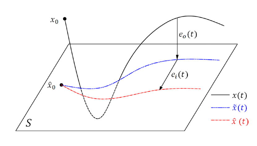
The error of the reduced model formed by the Galerkin projection can be defined as $e(t):=\hat{x}(t)-x(t)$. Let $e_{o}(t):=(I_{k}-P)e(t)$, which denotes the error component orthogonal to $S$, and $e_{i}(t):=Pe(t)$, which denotes the component of error parallel to $S$ (see Figure 1). Thus, we have

(5) $$e_{o}(t)=\tilde{x}(t)-x(t),$$

which directly comes from the projection. However, since the system is evolutionary with time, further approximations of the projection-based reduced model result in an additional error $e_{i}(t)$, and we have

(6) $$e_{i}(t)=\hat{x}(t)-\tilde{x}(t).$$

Although $e_{i}(t)$ and $e_{o}(t)$ are orthogonal to each other, they are not independent [19].

Figure 1: Illustration of the actual solution $x(t)$ for the original system (1), the projected solution $\tilde{x}(t)$ on $S$, and the approximate solution $\hat{x}(t)$ computed by the reduced model (3). The component of error orthogonal to $S$ is given by $e_{o}(t)=\tilde{x}(t)-x(t)$ and the component of error parallel to $S$ is given by $e_{i}(t)=\hat{x}(t)-\tilde{x}(t)$. This figure is reproduced from [19].

Lemma 3.

Consider the initial value problem (1) over the interval $J_{0}=[0,a/2]$. $a$, $J_{a}$, $b$, $B_{b}(x_{0})$, $M$, $P$, $x(t)$, $\tilde{x}(t)$, $\hat{x}(t)$, $e(t)$, $e_{o}(t)$, and $e_{i}(t)$ are defined as above. Suppose $f(t,x)$ is a uniformly Lipschitz function of $x$ with constant $K$ and a continuous function of $t$ for all $(t,x)\in J_{a}\times B_{b}(x_{0})$. Then the error $e(t)=\hat{x}(t)-x(t)$ in the infinity norm for the interval $J_{0}$ is bounded by

(7) $$\left\|e\right\|_{\infty}\leq e^{Ka/2}\left\|e_{o}\right\|_{\infty}+e^{Ka/2}\left\|{e_{i}(0)}\right\|.$$

Proof.

Since $f(t,x)$ is a uniformly Lipschitz function for any $(t,x)\in J_{a}\times B_{b}(x_{0})$, Lemmas 1 and 2 respectively imply the unique existences of $x(t)\in B_{b}(x_{0})$ and $\hat{x}(t)\in B_{b}(x_{0})$. Moreover, we can uniquely determine $\tilde{x}(t)\in B_{b}(x_{0})$ by $\tilde{x}(t)=Px(t)$. Therefore, $x(t)$, $\tilde{x}(t)$, and $\hat{x}(t)$ are all well-defined for any $t\in J_{0}$.

Substituting (1) and (3) into the differentiation of $e_{o}(t)+e_{i}(t)=\hat{x}(t)-x(t)$ yields

(8) $$\dot{e}_{o}+\dot{e}_{i}=Pf(t,\hat{x})-f(t,x).$$

Left multiplying (8) by $P$, expanding $\hat{x}$, and recognizing that $P^{2}=P$ gives

$$\dot{e}_{i}(t)=P(f(t,x+e_{o}+e_{i})-f(t,x)).$$

Using this equation by expanding $\left\|e_{i}(t+h)\right\|$ and applying triangular inequality yields

$$\begin{array}[]{l}\left\|{{e_{i}}(t+h)}\right\|=\left\|{{e_{i}}(t)+hPf(t,x+{e_{o}}+{e_{i}})-hPf(t,x)}\right\|+\mathcal{O}({h^{2}})\vskip 3.0pt plus 1.0pt minus 1.0pt\\ \ \ \ \ \ \ \ \ \ \ \ \ \ \ \ \leq\left\|{{e_{i}}(t)}\right\|+h\left\|{Pf(t,x+{e_{o}}+{e_{i}})-Pf(t,x+{e_{o}})}\right\|\vskip 3.0pt plus 1.0pt minus 1.0pt\\ \ \ \ \ \ \ \ \ \ \ \ \ \ \ \ \ \ \ \ \ \ \ \ +h\left\|{Pf(t,x+{e_{o}})-Pf(t,x)}\right\|+\mathcal{O}({h^{2}}).\end{array}$$

Rearranging this inequality and applying the Lipschitz conditions gives

$$\frac{{\left\|{{e_{i}}(t+h)}\right\|-\left\|{{e_{i}}(t)}\right\|}}{h}\leq K\left\|{{e_{i}}(t)}\right\|+K\left\|{{e_{o}}(t)}\right\|+\mathcal{O}(h).$$

Since $\mathcal{O}(h)$ can be uniformly bounded independent of $e_{i}(t)$, using the mean value theorem and letting $h\to 0$ give

$$\frac{{\rm{d}}}{{{\rm{d}}t}}\left\|{{e_{i}}(t)}\right\|\leq K\left\|{{e_{i}}(t)}\right\|+K\left\|{{e_{o}}(t)}\right\|.$$

Rewriting the above inequality into integral form, $\left\|{{e_{i}}(t)}\right\|\leq\alpha(t)+K\int_{0}^{t}{\left\|{{e_{i}}(\tau)}\right\|{\rm{d}}\tau}$, where $\alpha(t):=\left\|{{e_{i}}(0)}\right\|+K\int_{0}^{t}{\left\|{{e_{o}}(\tau)}\right\|{\rm{d}}\tau}$, and using Gronwall’s lemma, we obtain

$$\left\|{{e_{i}}(t)}\right\|\leq\alpha(t)+\int_{0}^{t}{\alpha(s)K\exp\left({\int_{s}^{t}{Kd\tau}}\right){\rm{ds}}}.$$

By definition, ${\left\|{{e_{o}}}\right\|_{\infty}}\geq\left\|{{e_{o}}(t)}\right\|$ for any $t\in J_{0}$. It follows that $\alpha(t)\leq\left\|{{e_{i}}(0)}\right\|+Kt\left\|{{e_{o}}}\right\|_{\infty}$. Simplifying the integral of the right-hand side of the above inequality gives

$${\left\|{{e_{i}}}(t)\right\|}\leq(e^{Ka/2}-1){\left\|{{e_{o}}}\right\|_{\infty}}+e^{Ka/2}\left\|{{e_{i}}(0)}\right\|,$$

for any $t\in J_{0}$. Combining the above inequality with $\left\|{e}\right\|_{\infty}\leq\left\|{e_{i}}\right\|_{\infty}+\left\|{e_{o}}\right\|_{\infty}$, one can obtain (7).  ∎

Remark: The above lemma provides a bound for $\|e_{i}(t)\|$ in terms of $\|e_{o}\|_{\infty}$ and $\|e_{i}(0)\|$. We have $\left\|e_{i}(0)\right\|=0$ when the initial condition of the reduced model is given by $\hat{x}_{0}=Px_{0}$ for (3). In this situation, (7) becomes ${\left\|{{e}}\right\|_{\infty}}\leq e^{Ka/2}{\left\|{{e_{o}}}\right\|_{\infty}}$. Considering $\left\|{e}\right\|_{\infty}\geq\left\|{e_{o}}\right\|_{\infty}$, $\left\|{e}\right\|_{\infty}=0$ holds if and only if $\left\|{e_{o}}\right\|_{\infty}=0$.

Obviously, $J_{0}$ is not the maximal time interval of the existence and uniqueness of $x(t)$ and $\hat{x}(t)$. For convenience, we simply assume that $x(t)$ and $\hat{x}(t)$ globally exist on $J=[0,T]$ throughout the rest of this article. Otherwise, we can shrink $J$ to a smaller interval, which starts from $0$, such that both $x(t)$ and $\hat{x}(t)$ are well-defined on $J$. Let $\mathcal{D}$ be an open set that contains $x(t)$, $\tilde{x}(t)$, and $\hat{x}(t)$ for all $t\in J$. Under this assumption, Lemma 3 is still valid if $J_{0}$ and $B_{b}(x_{0})$ are substituted by $J$ and $\mathcal{D}$, respectively.

2.2 POD

In order to provide an accurate description for the original system, the POD method can be used to deliver a set of empirical eigenfunctions such that the error for representing the given data onto the spanned subspace is optimal, in a least squares sense [11]. Assume that $m$ precomputed snapshots form a matrix, $X:=[x(t_{1}),...,x(t_{m})]$. Then, the truncated singular value decomposition (SVD)

(9) $$X\approx\Phi\Lambda\Psi^{T}$$

provides the POD basis matrix $\Phi\in\mathbb{R}^{n\times k}$, where $\Lambda\in\mathbb{R}^{k\times k}$ is a diagonal matrix that consists of the first $k$ nonnegative singular values arranged in decreasing order. $P$ is then obtained by $\Phi\Phi^{T}$.

Let $E$ denote the energy of the full system, which is approximated by the square of the Frobenius norm of snapshot matrix $X$, $E=\int_{{0}}^{{T}}{{{\left\|{x(t)}\right\|}^{2}}\>\mathrm{d}t}\approx\|X\|_{F}^{2}=\sum\nolimits_{\alpha=1}^{r}{\lambda_{\alpha}^{2}}$, where $r=\min(n,m)$. Let $E^{\prime}$ denote the energy in the optimal $k$-dimensional subspace, $E^{\prime}=\int_{{0}}^{{T}}{{{\left\|{{P}x(t)}\right\|}^{2}}\>\mathrm{d}t}\approx\|PX\|_{F}^{2}=\sum\nolimits_{\alpha=1}^{k}{\lambda_{\alpha}^{2}}$. A criterion can be set to limit the approximation error in the energy by a certain fraction $\eta$. Then, we seek $k\ll r$ so that

(10) $${{E^{\prime}}\mathord{\left/{\vphantom{{E^{\prime}}E}}\right.\kern-1.2pt}E}>\eta.$$

The key for POD and other projection-based reduced models is to find a subspace where all the state vectors approximately reside. Although these methods can significantly increase the computational speed during the online stage, the cost of data ensemble construction in the offline stage is often very expensive. For these reasons, developing an inexpensive online manifold learning technique is a desirable objective.

3 SIRM

The SIRM method is introduced by combining subspace iteration with a model reduction procedure in this section. The idea of subspace construction is to enhance the POD method by feeding it with information drawn from the observed state of the system and its time derivation. Then, a more precise solution is solved by projecting the original system onto this subspace. The subspace construction is carried out iteratively until a convergent solution is achieved.

3.1 Algorithm of SIRM

In this article, a $k$-dimensional subspace $S$ is called invariant of $x(t)$ (or invariant for short) if $x(t)\in S$ for all $t\in J$. In this case, $Px(t)=x(t)$, which means that $P$ is an invariant projection operator on the trajectory and that $\tilde{x}(t)=x(t)$. As mentioned above, $e_{o}(t)=0$ holds if and only if $e(t)=0$. Then, $\hat{x}(t)=x(t)$. Inserting (1) and (3) into $\dot{\hat{x}}(t)=\dot{x}(t)$, one can achieve $Pf(t,x)=f(t,x)$, which is equivalent to $f(t,x)\in S$. In fact, $(x(t),f(t,x))$ can be considered a point in the tangent bundle $TS$, which coincides with the Cartesian product of $S$ with itself. As an invariant projection, $P$ preserves not only the state vectors along the solution orbit but also the associated tangent vectors, i.e., the dynamics.

On the $j$th iteration, the aim is to construct a subspace $S^{j}$ such that both $\hat{x}^{j-1}$ and $f(t,\hat{x}^{j-1})$ are invariant under the associated projection operator $P^{j}$, i.e.,

(11) $$P^{j}(\hat{x}^{j-1})=\hat{x}^{j-1},$$

(12) $$P^{j}(f(t,\hat{x}^{j-1}))=f(t,\hat{x}^{j-1}).$$

Thus, both $\hat{x}^{j-1}(t)$ and $f(t,\hat{x}^{j-1}(t))$ reside in $S^{j}$ for all $t\in J=[0,T]$.

If the solution orbit is given at discrete times $t_{1},...,t_{m}$, then we have an $n\times m$ state matrix

(13) $$\hat{X}^{j}:=[\hat{x}^{j}(t_{1}),...,\hat{x}^{j}(t_{m})].$$

Accordingly, the samples of tangent vectors along the approximating orbit can form another $n\times m$ matrix,

(14) $$\hat{F}^{j}:=[f(t_{1},\hat{x}^{j}(t_{1})),...,f(t_{m},\hat{x}^{j}(t_{m}))].$$

A combination of $\hat{X}^{j}$ and $\hat{F}^{j}$ gives an information matrix, which is used to represent an extended data ensemble

(15) $$\hat{Y}^{j}:=[\hat{X}^{j},\gamma\hat{F}^{j}],$$

where $\gamma$ is a weighting coefficient. The basis vectors of $S^{j}$ can be obtained by using SVD of $\hat{Y}^{j-1}$. $\gamma=1$ is a typical value that is used to balance the truncation error of $\hat{X}^{j}$ and $\hat{F}^{j}$. It can be noted that a large $m$ value will lead to intensive computation, but the selected snapshots should reflect the main dimensions of states and tangent vectors along the solution trajectory. When the width of each time subinterval (partitioned by $t_{i}$) approaches zero, $S^{j}$ can be given by the column space of $\hat{Y}^{j-1}$.

Algorithm 1 SIRM

0:  The initial value problem (1).

0:  An approximate solution $\hat{x}(t)$.

  Set a test function $\hat{x}^{0}(t)$ as the trial solution. Initialize the iteration number $j=0$.

  repeat

     1: Update the iteration number $j=j+1$.

     2: Assemble snapshots of an approximate solution $\hat{x}^{j-1}(t)$ into matrix form $\hat{X}^{j-1}$.

     3: Compute vector field matrix $\hat{F}^{j-1}$ associated with snapshots in $\hat{X}^{j-1}$.

     4: Form an information matrix for the extended data ensemble $\hat{Y}^{j-1}=[\hat{X}^{j-1},\gamma\hat{F}^{j-1}]$.

     5: Based on $\hat{Y}^{j-1}$, compute the empirical eigenfunctions $\Phi^{j}$ through POD.

     6: Project the original equation onto a linear subspace spanned by $\Phi^{j}$ and form a reduced model.

     7: Solve the reduced model and obtain an approximate solution $z^{j}(t)$ in the subspace coordinate system.

     8: Express the updated solution in the original coordinate system $\hat{x}^{j}(t)=\Phi^{j}z^{j}(t)$.

  until $\left\|\hat{x}^{j}-\hat{x}^{j-1}\right\|_{\infty}<\epsilon$, where $\epsilon$ is the error tolerance.

  Obtain the final approximate solution $\hat{x}(t)=\hat{x}^{j}(t)$.

Algorithm 1 lists the comprehensive procedures of the SIRM method. A new subspace $S^{j}$ is constructed in each iteration, followed by an approximate solution $\hat{x}^{j-1}(t)$. As $\hat{x}^{j}(t)\to x(t)$, $S^{j}$ approaches an invariant subspace. For this reason, SIRM is an iterative manifold learning procedure, which approximates an invariant subspace by a sequence of subspaces. A complete iteration cycle begins with a collection of snapshots from the previous iteration (or an initial test function). Then, a subspace spanned by an information matrix is constructed. Empirical eigenfunctions are generated by POD, and finally a reduced-order equation obtained by Galerkin projection (2) is solved.

3.2 Convergence Analysis

In this subsection, we first provide a local error bound for the sequence of approximate solutions $\{\hat{x}^{j}(t)\}$ obtained by SIRM, which paves the way for the proof of local and global convergence of the sequence.

It can be noted that both $x^{j-1}(t)\in S^{j}$ and $f(t,x^{j-1})\in S^{j}$ hold for all $t\in J_{0}$ only in an ideal situation. If $S^{j}$ is formed by extracting the first few dominant modes from the information matrix of the extended data ensemble (15), neither (11) nor (12) can be exactly satisfied. Let $\varepsilon^{j}$ quantify the projection error,

(16) $$\varepsilon^{j}:=\int_{{0}}^{a/2}{{{\left\|{\left({I-{P^{j}}}\right){{\hat{x}}^{j-1}}(\tau)}\right\|}^{2}}\>\mathrm{d}\tau+}\gamma^{2}\int_{{0}}^{a/2}{{{\left\|{\left({I-{P^{j}}}\right)f(\tau,{{\hat{x}}^{j-1}})}\right\|}^{2}}\>\mathrm{d}\tau}.$$

If SVD is used to construct the empirical eigenfunctions, $\varepsilon^{j}$ can be estimated by

(17) $$\varepsilon^{j}\approx\sum\limits_{\alpha=k^{j}+1}^{r}{(\lambda_{\alpha}^{j})^{2}},$$

where $\lambda_{\alpha}^{j}$ is the $\alpha$th singular value of the information matrix $\hat{Y}^{j-1}$, and $k^{j}$ is the adaptive dimension of $S^{j}$ such that the truncation error produced by SVD is bounded by $\varepsilon^{j}\leq\varepsilon$. The following lemma gives an error bound for the limit of the sequence $\{\hat{x}^{j}(t)\}$.

Lemma 4.

Consider solving the initial value problem (1) over the interval $J_{0}=[0,a/2]$ by the SIRM method. $a$, $J_{a}$, $b$, $B_{b}(x_{0})$, $M$, $P$, $x(t)$, $\tilde{x}(t)$, $\hat{x}(t)$, $e(t)$, $e_{o}(t)$, and $e_{i}(t)$ are defined as above. The superscript $j$ denotes the $j$th iteration. Suppose $f(t,x)$ is a uniformly Lipschitz function of $x$ with constant $K$ and a continuous function of $t$ for all $(t,x)\in J_{a}\times B_{b}(x_{0})$. Then $\{\hat{x}^{j}(t)\}$ approaches $x(t)$ with an upper bound of $\left\|e\right\|_{\infty}$ given by

(18) $$\chi=\frac{{\sqrt{a\varepsilon}{e^{Ka/2}}}}{{{\sqrt{2}\gamma}(1-Ka{e^{Ka/2}}/2)}}+\frac{2\theta e^{Ka/2}}{{1-Ka{e^{Ka/2}}/2}}$$

for all $t\in J_{0}$ provided that

(19) $$a<\min\left[\frac{b}{M},\frac{2e^{-Kb/2M}}{K}\right],$$

where $\theta$ is the maximal error of the initial states in reduced models, and $\theta<b/2$.

Proof.

As proved in Lemma 3, $x(t)$, $\tilde{x}(t)$, and $\hat{x}(t)$ are well-defined over the interval $J_{0}$. Moreover, $x(t)$, $\tilde{x}(t)$, and $\hat{x}(t)\in B_{b}(x_{0})$ for all $t\in J_{0}$. Multiplying (8) on the left by $I-P^{j}$, we obtain the evolution equation for $e_{o}^{j}(t)$,

$$\dot{e}^{j}_{o}=-(I-P^{j})f(t,x),$$

which is equivalent to

(20) $$\dot{e}_{o}^{j}=(I-{P^{j}})[f(t,x+{e^{j-1}})-f(t,x)]-(I-{P^{j}})f(t,x+{e^{j-1}}).$$

Considering that $x(t)\in B_{b}(x_{0})$, $\hat{x}^{j-1}(t)\in B_{b}(x_{0})$ for all $t\in J_{0}$ and $f(t,x)$ is a uniformly Lipschitz function for all $(t,x)\in J_{a}\times B_{b}(x_{0})$ with constant $K$, it follows that

(21) $$\left\|{f(t,x+e^{j-1})-f(t,x)}\right\|\leq K\left\|{e^{j-1}(t)}\right\|.$$

Since $P^{j}$ is a projection matrix, we have $\left\|I-P^{j}\right\|=1$. This equation together with (20) and (21) yields

(22) $$\left\|\dot{e}_{o}^{j}(t)\right\|\leq K\left\|{{e^{j-1}}(t)}\right\|+\left\|{(I-{P^{j}})f(t,x+{e^{j-1}})}\right\|.$$

For $h>0$, the expansion of $e_{o}^{j}(t+h)$ gives

(23) $$\left\|{e_{o}^{j}(t+h)}\right\|\leq\left\|{e_{o}^{j}(t)}\right\|+h\left\|{\dot{e}_{o}^{j}(t)}\right\|+\mathcal{O}(h^{2}).$$

Rearranging (23) and applying (22) results in

(24) $$\frac{{\left\|{e_{o}^{j}(t+h)}\right\|-\left\|{e_{o}^{j}(t)}\right\|}}{h}\leq K\left\|{{e^{j-1}}(t)}\right\|+\left\|{(I-{P^{j}})f(t,x+{e^{j-1}})}\right\|+\mathcal{O}(h),$$

where the $\mathcal{O}(h)$ term may be uniformly bounded independent of $e_{o}^{j}(t)$. Integrating (24) with respect to $t$ yields

(25) $$\left\|{e_{o}^{j}(t)}\right\|\leq K\int_{{0}}^{t}{\left\|{{e^{j-1}}(\tau)}\right\|\>\mathrm{d}\tau}+\int_{{0}}^{t}{\left\|{(I-{P^{j}})f(\tau,x+{e^{j-1}})}\right\|\>\mathrm{d}\tau}+\left\|e_{o}^{j}(0)\right\|.$$

For $t\in J_{0}$, the first term on the right-hand side is bounded by $Ka\left\|{{e^{j-1}}}\right\|_{\infty}$/2. Using the definition of $\varepsilon^{j}$ in (16) and the fact that $\varepsilon^{j}\leq\varepsilon$ for each $j$, we obtain

$$\varepsilon\geq\gamma^{2}\int_{{0}}^{a/2}{{{\left\|{\left({I-{P^{j}}}\right)f(\tau,{{\hat{x}}^{j-1}})}\right\|}^{2}}\>\mathrm{d}\tau}.$$

By the Cauchy–Schwarz inequality, the second term on the right-hand side of (25) is bounded by $\sqrt{a\varepsilon/2{\gamma^{2}}}$ when $t\leq a/2$. It follows that

$$\left\|{e_{o}^{j}(t)}\right\|\leq\frac{{Ka{{\left\|{{e^{j-1}}}\right\|}_{\infty}}}}{2}+\sqrt{\frac{{a\varepsilon}}{{2{\gamma^{2}}}}}+\left\|{e_{o}^{j}(0)}\right\|.$$

Using (7) in Lemma 3, this inequality yields

(26) $${\left\|{{e^{j}}}\right\|_{\infty}}\leq\frac{Ka{{{{{e^{Ka/2}}}}}}{\left\|{{e^{j-1}}}\right\|_{\infty}}}{2}+\frac{{\sqrt{a\varepsilon}e^{Ka/2}}}{{\sqrt{2}{\gamma}}}+e^{Ka/2}\left\|e_{o}^{j}(0)\right\|+e^{Ka/2}\left\|e_{i}^{j}(0)\right\|.$$

If the error of the initial condition is bounded by $\left\|e^{j}(0)\right\|\leq\theta$ for each iteration, then $\left\|e_{o}^{j}(0)\right\|\leq\theta$, and $\left\|e_{i}^{j}(0)\right\|\leq\theta$. As a result,

(27) $${\left\|{{e^{j}}}\right\|_{\infty}}\leq\frac{Ka{{{{{e^{Ka/2}}}}}}{\left\|{{e^{j-1}}}\right\|_{\infty}}}{2}+\frac{{\sqrt{a\varepsilon}e^{Ka/2}}}{{\sqrt{2}{\gamma}}}+2\theta e^{Ka/2}.$$

By (19), $Ka{{{{{e^{Ka/2}}}}}}/2<Ka{{{{{e^{Kb/2M}}}}}}/2<1$. Using the definition of $\chi$ in (18), (27) can be rewritten as

(28) $$\|e^{j}\|_{\infty}-\chi\leq Ka{{{{{e^{Ka/2}}}}}}/2(\|e^{j-1}\|_{\infty}-\chi).$$

It follows that if $\|e^{j}\|_{\infty}-\chi>0$ for all $j$, it converges to $0$ linearly. Otherwise, once $\|e^{j_{0}-1}\|_{\infty}-\chi\leq 0$ for some $j_{0}$, then $\|e^{j_{0}}\|_{\infty}\leq\chi$, and so does $\|e^{j}\|_{\infty}$ for all $j>j_{0}$. Therefore, we have

(29) $$\mathop{\limsup}\limits_{j\to+\infty}{\left\|{{e^{j}}}\right\|_{\infty}}\leq\chi,$$

which means $\left\|e^{j}(t)\right\|$ is bounded by $\chi$ as $j\to+\infty$ for all $t\in J_{0}$.  ∎

The first term of $\chi$ is introduced by the truncation error. By decreasing the width of time intervals among neighboring snapshots and increasing the number of POD modes, we can limit the value of $\varepsilon$. The second term of $\chi$ is the magnified error caused by $e^{j}(0)$. If both $\chi$ and $e^{j}(0)$ approach 0, we have the following theorem.

Theorem 5 (local convergence of SIRM).

Consider solving the initial value problem (1) over the interval $J_{0}=[0,a/2]$ by the SIRM method. $a$, $J_{a}$, $b$, $B_{b}(x_{0})$, $M$, $P$, $x(t)$, $\tilde{x}(t)$, $\hat{x}(t)$, $e(t)$, $e_{o}(t)$, and $e_{i}(t)$ are defined as above. The superscript $j$ denotes the $j$th iteration. Suppose $f(t,x)$ is a uniformly Lipschitz function of $x$ with constant $K$ and a continuous function of $t$ for all $(t,x)\in J_{0}\times B_{b}(x_{0})$. For each iteration, the reduced subspace $S^{j}$ contains $x_{0}$ and the initial state for the reduced model is given by $\hat{x}^{j}_{0}=P^{j}x_{0}$. Moreover, (12) is satisfied. Then the sequence $\{\hat{x}^{j}(t)\}$ uniformly converges to $x(t)$ for all $t\in J_{0}$, provided that

(30) $$a<\min\left[\frac{b}{M},\frac{2e^{-Kb/2M}}{K}\right].$$

Proof.

Since the initial state $\hat{x}^{j}_{0}$ is the projection of $x_{0}$ onto $S^{j}$, we have $e_{i}^{j}(0)=0$. Meanwhile, $x_{0}\in S^{j}$ results in $e_{o}^{j}(0)=0$. Then the initial error satisfies $e^{j}(0)=0$. On the other hand, (12) requires that $f(t,\hat{x}^{j-1})$ is invariant under the projection operator $P^{j}$, i.e., $(I-P^{j})f(t,\hat{x}^{j-1})=0$, which leads to $\varepsilon^{j}=0$. Therefore, in Lemma 4, both $\varepsilon$ and $\theta$ approach 0, and so does $\chi$. As a consequence, $\{\hat{x}^{j}(t)\}$ converges to the fixed point $x(t)$ for all $t\in J_{0}$.  ∎

It can be noted that the error bound $\chi$ of the SIRM method is completely determined by $\theta$ and $\varepsilon$. As an alternative to (15), a more straightforward form of the information matrix for the extended data ensemble can be written as

(31) $$\tilde{Y}^{j}:=[x_{0},\gamma\hat{F}^{j}],$$

and the SIRM method can still converge to $x(t)$ by Theorem 5. However, as a Picard-type iteration, SIRM can only be guaranteed to reduce local error within one iteration. If $\varepsilon$ and $\theta$ approach 0, (27) can be rewritten as

(32) $$\frac{{{{\left\|{{e^{j}}}\right\|}_{\infty}}}}{{{{\left\|{{e^{j-1}}}\right\|}_{\infty}}}}\leq\frac{Ka{e^{Ka/2}}}{2}.$$

When the interval $J_{0}$ is large, for example, $a>2/K$, the left-hand side might be greater than $1$. Thus, although $\hat{x}^{j}(t)$ has less local error than $\hat{x}^{j-1}(x)$, it might be less accurate in a global sense.

On the other hand, if the information matrix (15) is applied to the SIRM method, $\hat{x}^{j-1}(t)\in S^{j}$ is satisfied for each iteration. For any $t$, $\left\|{e_{o}^{j}(t)}\right\|$ denotes the distance from $x(t)$ to $S^{j}$, while $\left\|e^{j-1}(t)\right\|$ denotes the distance from $x(t)$ to $\hat{x}^{j-1}(t)$. Recognizing that $\hat{x}^{j-1}(t)\in S^{j}$, we have

(33) $$\left\|{e_{o}^{j}(t)}\right\|\leq\left\|e^{j-1}(t)\right\|.$$

If $\theta$ approaches 0, so does $\|e_{i}^{j}(0)\|$. Using (7) in Lemma 3, one obtains

(34) $$\frac{{{{\left\|{{e^{j}}}\right\|}_{\infty}}}}{{{{\left\|{{e^{j-1}}}\right\|}_{\infty}}}}\leq{e^{Ka/2}}.$$

This inequality still cannot guarantee that $\left\|e^{j-1}(t)\right\|<\left\|e^{j}(t)\right\|$ for all $t\in J$. However, when $a>2/K$ it provides a stronger bound than (32) does, which can effectively reduce the global error.

So far, we have proved convergence of SIRM for a local time interval $J_{0}=[0,a/2]$. Since the estimates used to obtain $J_{0}$ are certainly not optimal, the true convergence time interval is usually much larger. Supposing $J_{0}\subset J$, we will next prove that the convergence region $J_{0}$ can be extended to $J$ under certain conditions.

Theorem 6 (global convergence of SIRM).

Consider solving the initial value problem (1) over the interval $J=[0,T]$ by the SIRM method. $P$, $x(t)$, $\tilde{x}(t)$, $\hat{x}(t)$, $e(t)$, $e_{o}(t)$, and $e_{i}(t)$ are defined as above. The superscript $j$ denotes the $j$th iteration. Suppose $f(t,x)$ is a locally Lipschitz function of $x$ and a continuous function of $t$ for all $(t,x)\in J\times\mathcal{D^{\prime}}$, where $\mathcal{D^{\prime}}$ is an open set that contains $x(t)$ for all $t\in J$. For each iteration, the reduced subspace $S^{j}$ contains $x_{0}$ and the initial state for the reduced model is given by $\hat{x}^{j}_{0}=P^{j}x_{0}$. Moreover, (12) is satisfied. The sequence $\{\hat{x}^{j}(t)\}$ then uniformly converges to $x(t)$ for all $t\in J$.

Proof.

Since $\mathcal{D^{\prime}}$ is open, there exists a constant $b$ such that $b>0$, and $\mathcal{E}:=\cup_{t}{\bar{B}_{b}}(x(t))\subset\mathcal{D^{\prime}}$. Since $f(t,x)$ is locally Lipschitz on $J\times\mathcal{D^{\prime}}$ and $\mathcal{E}$ is compact, $f(t,x)$ is Lipschitz on $J\times\mathcal{E}$. Let $K$ denote the Lipschitz constant for $(t,x)\in J\times\mathcal{E}$. In addition, we can choose the value of $a$, which is bounded by (30). Let $J_{m}$ be the maximal interval in $J$ such that for all $t\in J_{m}$, $\hat{x}^{j}(t)\to x(t)$ uniformly as $j\to\infty$. Theorem 5 indicates that SIRM will generate a sequence of functions $\{\hat{x}^{j}(t)\}$ that uniformly converges to $x(t)$ for all $t\in J_{0}=[0,a/2]$. For this reason, we have $J_{0}\subset J_{m}$.

Now assume $J_{m}\neq J$. Then, there exists a $t_{i}\in J_{m}$ such that $t_{i}+a/2\leq T$, but $t_{i}+a/2\notin J_{m}$. $t_{i}\in J_{m}$ means for every $\kappa>0$ there exists an integer $M_{1}(\kappa)>0$ such that for all $j$ with $j>M_{1}(\kappa)$, $\hat{x}^{j}(t_{i})$ uniquely exists and $\left\|\hat{x}^{j}(t_{i})-x(t_{i})\right\|<\kappa$.

Consider the initial value problem

(35) $$\dot{y}=f(t,y);\ \ \ \ \ y(0)=y_{0}=x(t_{i}).$$

The corresponding reduced model of SIRM at iteration $l$ is given by

(36) $$\dot{\hat{y}}^{l}=P^{l}f(t,\hat{y}^{l});\ \ \ \ \ \hat{y}^{l}(0)=y_{0}+e^{l}(t_{i}),$$

where $e^{l}(t_{i})=\hat{x}^{l}(t_{i})-x(t_{i})$. For an arbitrary small positive number $\kappa^{\prime}$, Lemma 4 implies that there exists a positive integer $M_{2}(\kappa^{\prime})$ such that whenever $l>M_{2}(\kappa^{\prime})$ and $t\in J_{0}=[0,a/2]$,

$$\left\|\hat{y}^{l}(t)-y(t)\right\|<\chi+\kappa^{\prime}.$$

Plugging $\chi$ from (18) into this inequality and replacing $\theta$ by $\kappa$, we have

(37) $$\left\|\hat{y}^{l}(t)-y(t)\right\|\leq\frac{{\sqrt{a\varepsilon}{e^{Ka/2}}}}{{{\sqrt{2}\gamma}(1-Ka{e^{Ka/2}}/2)}}+\frac{2\kappa e^{Ka/2}}{{1-Ka{e^{Ka/2}}/2}}+\kappa^{\prime}.$$

In an ideal case, the truncation error is zero, i.e., $\varepsilon=0$. Then, the right-hand side of (37) can be arbitrarily small. The uniqueness lemma for ODE’s (Lemma 1) yields $y(t)=x(t_{i}+t)$ and $\hat{y}^{j}(t)=\hat{x}^{j}(t_{i}+t)$. Therefore, for every $\epsilon>0$, there exists an integer

(38) $$N(\epsilon)=M_{1}\left({\frac{{(1-Ka{e^{Ka/2}}/2)\epsilon}}{{4e^{Ka/2}}}}\right)+M_{2}\left({\frac{\epsilon}{2}}\right)$$

such that, as long as $j>N(\epsilon)$, $\left\|\hat{x}^{j}(t)-x(t)\right\|\leq\epsilon$ holds for all $t\in[0,t_{i}+a/2]$. Moreover, $t_{i}+a/2\leq T$. However, this contradicts our assumption that $t_{i}+a/2\notin J_{m}$. Therefore, $J_{m}=J$, i.e., $\hat{x}^{j}(t)$ uniformly converges to $x^{t}(t)$ for all $t\in J$.  ∎

3.3 Computational complexity

The computational complexity of the SIRM method for solving an initial value problem is discussed in this subsection. We follow [19] when we estimate the computational cost of the procedures related to the standard POD-Galerkin approach.

Let $\gamma(n)$ be the cost of computing the original vector field $f(t,x)$, and let $\hat{\gamma}(k,n)$ be the cost of computing the reduced vector field $\Phi^{T}f(t,\Phi z)$ based on the POD-Galerkin approach. In the full model, the cost of one-step time integration using Newton iteration is given by $b\gamma(n)/5+b^{2}n/20$ if all $n\times n$ matrices are assumed to be banded and have $b+1$ entries around the diagonal [19]. Thus, the total cost of the full model for $N_{T}$ steps is given by

(39) $$N_{T}\cdot\left(b\gamma(n)/5+b^{2}n/20\right).$$

Next, we analyze the complexity of Algorithm 1. Assuming a trial solution is given initially, the computational cost for each iteration mainly involves the following procedures. In procedure 3, an $n\times m$ vector field matrix, $\hat{F}^{j-1}$, is computed based on $m$ snapshots. In procedure 5, from an $n\times 2m$ information matrix, $\hat{Y}^{j-1}$, the empirical eigenfunctions $\Phi^{j}$ can be obtained in $4m^{2}n$ operations by SVD [25]. In procedure 6, the original system is projected onto a subspace spanned by $\Phi^{j}$, and this cost is denoted by $\beta(k,n)$. For a linear time-invariant system, $\dot{x}=Ax$, $\beta(k,n)$ represents the cost to compute $(\Phi^{j})^{T}A\Phi^{j}$, which is given by $bnk$ for sparse $A$. For a general system, $\beta(k,n)$ is a nonlinear function of $n$. In procedure 7, the reduced model is evolved for $N_{T}$ steps by an implicit scheme to obtain $z^{j}(t)$. If the reduced model inherits the same scheme from the full model, then one-step time integration needs $k\hat{\gamma}(k,n)/5+k^{3}/15$ operations [19]. In procedure 8, an $n\times m$ snapshot matrix $\hat{X}^{j}(t)$ is constructed through $\hat{x}(t_{i})=\Phi z(t_{i})$. Table 1 shows the asymptotic complexity for each basic procedure mentioned above. Let $N_{I}$ denote the number of iterations; then, the total cost of Algorithm 1 is given by

(40) $$N_{I}\cdot\left(4m^{2}n+\beta(k,n)+N_{T}\cdot\left(k\hat{\gamma}(k,n)/5+k^{3}/15\right)+m\gamma(n)+mnk\right).$$

Notice that the first three terms in (40) represent the cost for the classic POD-Galerkin method, while construction of the extended data ensemble needs extra computational overhead, $m\gamma(n)+mnk$, for each iteration. On one hand, the subspace dimension $k$ is no greater than the number of sampling points $m$, which means $mnk<4m^{2}n$. On the other hand, we can always choose an optimal $m$ value such that $m\ll N_{T}$. Thus, the extra computational overhead plays a secondary role in (40), and the computational complexity of Algorithm 1 is approximately equal to the number of iterations, $N_{I}$, multiplied by the cost of the standard POD-Galerkin approach.

Table 1: Complexity of Algorithm 1 for one iteration using an implicit scheme for time integration

Procedure	Complexity
Compute a vector field matrix $\hat{F}^{j-1}$	$m\gamma(n)$
SVD: empirical eigenfunctions $\Phi^{j}$	$4m^{2}n$
Construct a reduced model	$\beta(k,n)$
Evolve the reduced model	$N_{T}(k\hat{\gamma}(k,n)/5+k^{3}/15)$
Obtain an approximate solution $\hat{X}^{j}$	$mnk$

Algorithm 1 does not explicitly specify the trial solution $\hat{x}^{0}(t)$. In fact, the convergence of SIRM does not depend on $\hat{x}^{0}(t)$, as previously shown. Thus, we can simply set $\hat{x}^{0}(t)$ as a constant, i.e., $\hat{x}^{0}(t)=x_{0}$. However, a “good” trial solution could lead to a convergent solution in fewer iterations and could thus decrease the total computational cost. For example, if the full model is obtained by a finite difference method with $n$ grid points and time step $\delta t$, a trial solution could be obtained by a coarse model, using the same scheme but $n/10$ grid points with time step $10\times\delta t$. Thus, the coarse model can cost less than $1\%$ of the required operations in the full model.

Notice that $\hat{\gamma}(k,n)\ll\gamma(n)$ is achieved only when the analytical formula of $\Phi^{T}f(t,\Phi z)$ can be significantly simplified, especially when $f(t,x)$ is a low-degree polynomial of $x$ [19]. Otherwise, it is entirely possible that the reduced model could be more expensive than the original one. Because of this effect, there is no guarantee that Algorithm 1 can speed up a general nonlinear system. However, it should be emphasized that the POD-Galerkin approach is not the only method that can be used to construct a reduced model in the framework of SIRM; in principle, it can be substituted by a more efficient model reduction technique when $f(t,x)$ contains a nonlinear term, such as trajectory piecewise linear and quadratic approximations [20, 21, 26, 6], the empirical interpolation method [10], or its variant, the discrete empirical interpolation method [5]. This article, however, focuses on using SIRM to obtain an accurate solution without a precomputed database. Therefore, the numerical simulations in the next subsection are still based on the classic POD-Galerkin approach.

3.4 Numerical Results

The proposed algorithm, SIRM, is illustrated in this subsection by a linear advection-diffusion equation and a nonlinear Burgers equation. These examples focus on demonstrating the capability of SIRM to deliver accurate results using reduced models. We also show an application of SIRM for the posteriori error estimation of a coarse model.

3.4.1 Advection-Diffusion Equation

Let $u=u(t,x)$. Consider the one-dimensional advection-diffusion equation with constant moving speed $c$ and diffusion coefficient $\nu$,

(41) $$u_{t}=-cu_{x}+\nu u_{xx},$$

on space $x\in[0,1]$. Without loss of generality, periodic boundary conditions are applied,

(42) $$\begin{array}[]{l}u(t,0)=u(t,1),\\ u_{x}(t,0)=u_{x}(t,1).\\ \end{array}$$

The initial condition is provided by a cubic spline function,

(43) $$u(0,x)=\left\{\begin{array}[]{ccl}\vspace{3pt}1-\frac{3}{2}s^{2}+\frac{3}{4}s^{3}&\text{if }&0\leq s\leq 1,\\ \frac{1}{4}(2-s)^{3}&\text{if }&1<s\leq 2,\\ 0&\text{if }&s>2,\end{array}\right.$$

where $s=10\times|x-1/3|$. The fully resolved model is obtained through a high-resolution finite difference simulation with spatial discretization by $n$ equally spaced grid points. The advection term is discretized by the first-order upwind difference scheme with the explicit two-step Adams–Bashforth method for time integration, while the diffusion term is discretized by the second-order central difference scheme with the Crank–Nicolson method for time integration.

(a)

(b)

Figure 2: (a) The velocity profiles at $t=0$ and $t=0.5$ of the one-dimensional advection-diffusion equation with constant speed $c=0.5$ and diffusion coefficient $\nu=10^{-3}$. $n=500$ grid points are used to obtain the full model for the fixed space domain $[0,1]$. The trial solution is obtained by extracting the first 10 Fourier modes from a coarse model based on $k^{0}=20$ grid points. When $\eta=10^{-8}$, it takes one iteration for SIRM to obtain an accurate solution by 12 modes. (b) Convergence of SIRM for different $\eta$ and $k^{0}$ values. Plot of the maximal $L_{2}$ error, $\|e^{j}\|_{\infty}=\sup\{\|\hat{u}^{j}(t)-u(t)\|:t\in[0,0.5]\}$, between the benchmark solution $u(t)$ and the iterative solution $\hat{u}^{j}(t)$ for $t\in[0,0.5]$.

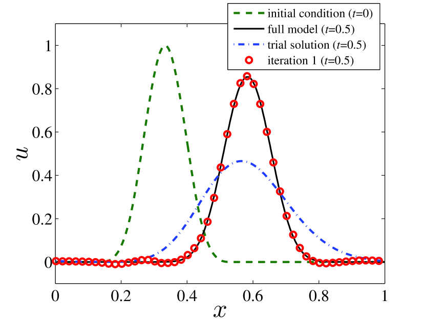
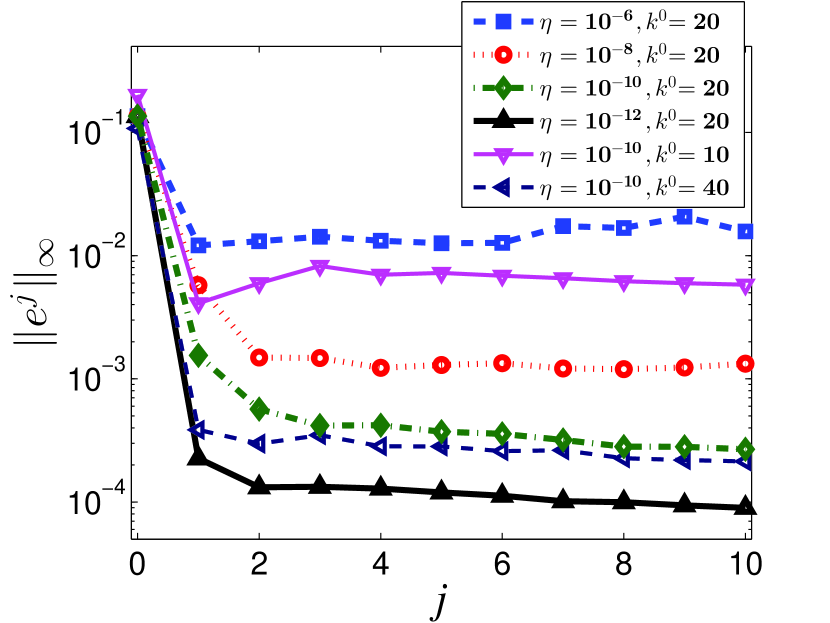
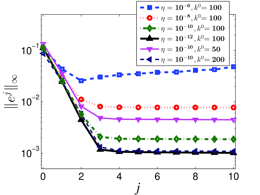
For our numerical experiments, we consider a system with $c=0.5$ and $\nu=10^{-3}$, which gives rise to a system with diffusion as well as advection propagating to the right. This can be seen in Figure 2(a), where the initial state and the final state (at $t=0.5$) are shown. The full model (reference benchmark solver) is computed through $n=500$ grid points. Thus, the unit step can be set as $\delta t=10^{-3}$ such that the Courant–Friedrichs–Lewy (CFL) condition is satisfied for the stability requirement, i.e., $c\delta t/\delta x\leq 1$. In order to initialize SIRM, a smaller simulation is carried out by the finite difference method with a coarse grid of $k^{0}=20$ and a larger time step of $2.5\times 10^{-2}$. In order to obtain a smooth function for the trial solution, the coarse solution is filtered by extracting the first $10$ Fourier modes. When $\eta=10^{-8}$, the full-order equation is projected onto a subspace spanned by $k=12$ dominant modes during the first iteration and a better approximation is obtained. For different $\eta$ and $k^{0}$ values, Figure 2(b) compares the maximal $L_{2}$ error between the benchmark solution $u(t)$ and the iterative solution $\hat{u}^{j}(t)$ for $t\in[0,0.5]$ in the first $10$ iterations. Each subspace dimension is adaptively determined by (10). If $k^{0}=20$, the first three iterations of SIRM respectively use 9, 9, and 11 dominant modes when $\eta=10^{-6}$; use 12, 14, and 14 dominant modes when $\eta=10^{-8}$; use 14, 17, and 18 dominant modes when $\eta=10^{-10}$; and use 17, 19, and 20 dominant modes when $\eta=10^{-12}$. As expected, a smaller $\eta$ value results in a smaller truncation error produced by SVD and the total error, $\|e^{j}\|_{\infty}$, for an approximate solution. Meanwhile, a trial solution with a higher initial dimension, $k^{0}$, could also significantly decrease the error for the first 10 iterations. It is also noted that $\|e^{j}\|_{\infty}$ is not a monotonically decreasing function of $j$, especially when $\eta=10^{-6}$ and $k^{0}=20$. This does not contradict the convergence analysis in the previous subsection. As a variant of the Picard iteration, the SIRM method achieves a better local solution in each iteration. As (34) indicates, we can only guarantee ${\left\|{{e^{j}}}\right\|}_{\infty}\leq{e^{Ka/2}{\left\|{{e^{j-1}}}\right\|}_{\infty}}$ in a global sense.

Before switching to the next numerical example, we compare the performance of SIRM with another online manifold learning technique, DIRM [18]. The DIRM method splits the whole system into $m_{n}$ subsystems. Starting with a trial solution, DIRM simulates each subsystem in turn and repeats this process until a globally convergent solution is obtained. For iteration $j$, DIRM connects the unreduced subsystem $i$ with the reduced versions of all other subsystems and simulates the resulting system

(44) $$\begin{array}[]{l}\dot{x}_{i}^{j}={f_{i}}(t,{X^{j}_{i}}),\\ \dot{z}_{l}^{j}=(\Phi_{l}^{j})^{T}{f_{l}}(t,{X^{j}_{i}}),\ \ \ \ \ \ \ \ \ \ l=1,...,i-1,i+1,...,m_{n},\\ \end{array}$$

where $X^{j}_{i}=[\Phi_{1}^{j}z_{1}^{j};...;\Phi_{i-1}^{j}z_{i-1}^{j};x_{i}^{j};\Phi_{i+1}^{j}z_{i+1}^{j};...;\Phi_{m_{n}}^{j}z_{m_{n}}^{j}]$. If $x_{i}^{j}\in\mathbb{R}^{n/m_{n}}$ and $z_{l}^{j}\in\mathbb{R}^{k}$, the reduced model of DIRM has a dimension of $m_{n}k+m/m_{n}$. Since DIRM reduces the dimension for each subsystem, rather than the original system, it inevitably keeps some redundant dimensions.

Table 2: The minimal subspace dimension of DIRM and SIRM that is required for solving the one-dimensional advection-diffusion equation when the error of the first iteration is smaller than $10^{-3}$, i.e., $\|e^{1}\|_{\infty}<10^{-3}$. Parameter values are $n=500$, $c=0.5$, $\delta t=10^{-3}$. The time domain is $[0,0.5]$. The trial solution is obtained by extracting the first 10 Fourier modes from a coarse simulation based on $20$ grid points.

	$\nu=10^{-1}$	$\nu=10^{-2}$	$\nu=10^{-3}$	$\nu=10^{-4}$
DIRM	92	92	116	116
SIRM	13	12	15	16

Table 2 compares the minimal subspace dimension of DIRM and SIRM that is required for solving (41) when the error of the first iteration is smaller than $10^{-3}$. We use all the aforementioned parameters except scanning $\nu$ from $10^{-1}$ to $10^{-4}$. For the DIRM application, the whole system with $n=500$ is divided into 25 subsystems, and the dimension of each subsystem is 20. When $\nu$ is greater than $10^{-2}$, the DIRM method uses three modes for each subsystem, and therefore the dimension of DIRM is $3\times 24+20=92$. When $\nu$ decreases to $10^{-3}$ and less, DIRM requires four modes for each system in order to maintain high accuracy, and the subspace dimension grows to $4\times 24+20=116$. Since SIRM requires fewer modes and simulates only one reduced system rather than 20 subsystems, it is much more efficient than DIRM for solving (41).

3.4.2 Viscous Burgers Equation

The viscous Burgers equation is similar to the advection-diffusion equation except, in the case of the viscous Burgers equation, the advection velocity is no longer constant. The general form of the one-dimensional Burgers equation is given by

(45) $$u_{t}=-uu_{x}+\nu u_{xx},$$

where $\nu$ is the diffusion coefficient. Let $\Omega=[0,1]$ denote the computational domain. Periodic boundary conditions (42) are applied. The cubic spline function (43) is used for the initial condition.

(a)

(b)

Figure 3: (a) The velocity profiles at $t=0$ and $t=1$ of the one-dimensional Burgers equation with constant diffusion coefficient $\nu=10^{-3}$. $n=2000$ grid points are used to obtain the full model for the fixed space domain $[0,1]$, while $k^{0}=100$ grids are used to obtain a coarse model. The first 10 Fourier modes are extracted to construct the trial solution. When $\eta=10^{-10}$, it takes three iterations for SIRM to obtain an accurate solution. (b) Convergence of SIRM for different $\eta$ and $k^{0}$ values. Plot of the maximal $L_{2}$ error, $\|e^{j}\|_{\infty}=\sup\{\|\hat{u}^{j}(t)-u(t)\|:t\in[0,1]\}$, between the benchmark solution $u(t)$ and the iterative solution $\hat{u}^{j}(t)$.

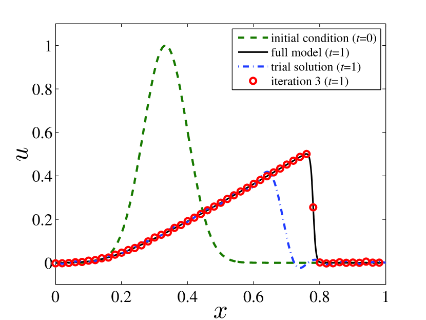
In the numerical simulation, the diffusion coefficient is given by $\nu=10^{-3}$. The full model is obtained using $n=2000$ grid points, while the trial solution is obtained by extracting the first $10$ Fourier modes from a coarse simulation with $k^{0}=100$ grid points. Because the one-dimensional Burgers equation has a positive velocity, a wave will propagate to the right with the higher velocities overcoming the lower velocities and creating steep gradients. This steepening continues until a balance with the dissipation is reached, as shown by the velocity profile at $t=1$ in Figure 3(a). Because states of the Burgers equation have high variability with time evolution, more modes are necessary in order to present the whole solution trajectory with high accuracy. Meanwhile, the SIRM method requires more iterations to obtain convergence.

The convergence plot for SIRM is shown in Figure 3(b). Equation (10) gives an adaptive dimension, $k$, in each iteration: their values are 21, 38, and 60 for the first three iterations when $\eta=10^{-6}$; are 26, 49, and 85 when $\eta=10^{-8}$; are 30, 62, and 105 when $\eta=10^{-10}$; and are 34, 76, and 129 when $\eta=10^{-12}$. When $\eta\leq 10^{-8}$, the error of the approximate solution decreases in the first few iterations and then converges to a fixed value, which is mainly determined by the truncation error produced by SVD. In order to achieve higher resolution, for each iteration, more snapshots are needed for each iteration to construct the information matrix and include more modes in the associated reduced model.

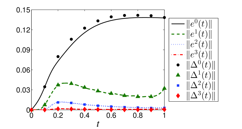
What is more, the SIRM method can be used to estimate errors of other approximate models as well. The Euclidean distance between the actual solution $u(t)$ and the approximate solution $\hat{u}^{0}(t)$ as a function of $t$ can indicate the accuracy of a coarse model (or a reduced model),

(46) $$\|e^{0}(t)\|=\|u(t)-\hat{u}^{0}(t)\|.$$

However, in many applications, the actual solution $u(t)$ is unknown or very expensive to obtain. In this case, the SIRM method can be used to obtain a more precise solution $\hat{u}^{1}(t)$, and the Euclidean distance between $\hat{u}^{1}(t)$ and $\hat{u}^{0}(t)$ can be used as an error estimator,

(47) $$\|\Delta^{0}(t)\|=\|\hat{u}^{1}(t)-\hat{u}^{0}(t)\|.$$

Although $\hat{u}^{1}(t)$ is only guaranteed to have higher accuracy than $\hat{u}^{0}(t)$ locally, (47) can be applied to identify whether and when the trial solution has a significant discrepancy from the actual solution. More generally, the error of the iterative solution $\hat{u}^{j}(t)$ computed by SIRM,

(48) $$\|e^{j}(t)\|=\|u(t)-\hat{u}^{j}(t)\|,$$

can (at least locally) be approximated by the difference between $\hat{u}^{j+1}(t)$ and $\hat{u}^{j}(t)$, as follows:

(49) $$\|\Delta^{j}(t)\|=\|\hat{u}^{j+1}(t)-\hat{u}^{j}(t)\|.$$

For this reason, the criterion $\left\|\hat{x}^{j}-\hat{x}^{j-1}\right\|_{\infty}<\epsilon$ is used in Algorithm 1 to indicate convergence of SIRM.

Revisiting the one-dimensional Burgers equation, Figure 4 shows that $\|\Delta^{j}(t)\|$ is a good approximation for the actual error $\|e^{j}(t)\|$ for $t\in[0,1]$.

Figure 4: Comparison of the actual error $\|e^{j}(t)\|=\|u(t)-\hat{u}^{j}(t)\|$ with the estimated error $\|\Delta^{j}(t)\|=\|\hat{u}^{j+1}(t)-\hat{u}^{j}(t)\|$ for $t\in[0,1]$, where $u(t)$ is the actual solution of the one-dimensional Burgers equation computed by $2000$ grid points, $\hat{u}^{0}(t)$ is the trial solution obtained by extracting the first 10 Fourier modes from a coarse simulation based on 100 grid points, and $\hat{u}^{j}(t)$ ($j\neq 0$) are iterative solutions computed by the SIRM method.

4 Local SIRM

In the previous section, the presented analysis and simulations illustrate that under certain conditions the SIRM method is able to obtain a convergent solution in the global time domain. However, the SIRM method still has existing redundancy with respect to both dimensionality and computation, as described in the following, that could be improved.

First, the reduced subspace formed by POD in SIRM keeps some redundant dimensions of the original system in each iteration. To explain this, consider a large-scale dynamical system whose solution exhibits vastly different states as it evolves over a large time horizon. In order to obtain a highly accurate representation for the entire trajectory, we need a subspace with relatively high dimensionality to form a surrogate model. However, projection-based model reduction techniques usually generate small but full matrices from large (but sparse) matrices. Thus, unless the reduced model uses significantly fewer modes, computing the reduced model could potentially be more expensive than computing the original one. Notice that the orbit of a dynamical system (1) is a one-dimensional curve; thus, it is desired that a local section of curve be embedded into a linear subspace of much lower dimensionality.

Second, for each iteration, SIRM requires that the entire trajectory be computed from the initial time to the final time of interest, $T$, which causes computational redundancy. As a variant of the Picard iteration, the rate of convergence of SIRM could be very slow for a nonlinear system with a large time domain. Under certain conditions, SIRM has a locally linear convergence. As inequality (28) indicates, when $t\in J_{0}$ the rate of convergence of $\|e^{j}\|_{\infty}-\chi$ is given by $Ka\exp(Ka/2)/2$. However, as (34) suggests, we cannot guarantee that SIRM could obtain a better global solution in each iteration. Meanwhile, if we have already obtained convergence at $t=a$ for some $0<a\leq T$, it would be a waste of computation to return to $t=0$ for the next iteration.

Thus, it is preferable to partition the entire time domain into several smaller subintervals, obtain a convergent solution for one subinterval, and then move forward to the next. A simple concept of time-domain partition was already introduced in [7] in the context of the standard POD-Galerkin method. As opposed to time domain partition, space domain partition [1] and parameter domain partition [8] also have be devolved to construct local reduced models using partial snapshots from a precomputed database. In this section, we combine the idea of time domain partition with SIRM and propose a local SIRM algorithm for model reduction. For each subinterval, the resulting method constructs a convergent sequence of approximating trajectories solved in subspaces of significantly lower dimensionality. Convergence analysis and the relation of the presented method with some other numerical schemes are also discussed. Then, we demonstrate its effectiveness in an example of the Navier–Stokes simulation of a lid-driven cavity flow problem.

4.1 Algorithm of Local SIRM

Suppose the entire time domain $J:=[0,T]$ is partitioned into $M$ smaller subintervals $J_{1},...,J_{M}$ with $J_{i}:=[t_{i-1},t_{i}]$. We slightly abuse the notation and denote the subinterval index by the subscript $i$. Let $t_{0}=0$ and $t_{M}=T$, such that $J=\cup_{i=1}^{M}{J_{i}}$. At subinterval $J_{i}$, the local solution trajectory approximately resides in a linear subspace $S_{i}$ spanned by column vectors in $\Phi_{i}$. Let $\Phi_{i}$ be orthonormal; then the reduced equation formed by the Galerkin projection is given by

(50) $$\dot{z}=\Phi_{i}^{T}f(t,\Phi_{i}z)$$

for $t\in J_{i}$. The SIRM method can be applied to approach a locally invariant subspace and obtain a convergent solution $x(t)$ for this subinterval. Specifically, we initially set a trial solution, $\hat{x}^{0}(t)$ for $t\in J_{i}$. During iteration $j$, an extended data ensemble, $\hat{Y}^{j-1}_{i}$, which contains a small number of snapshots within the subinterval, is constructed and then served to generate the empirical eigenfunctions of the subspace to be used in the next iteration cycle. After locally projecting the full model onto this subspace and constructing a reduced model through (50), the time integration is carried out in a low-dimensional space to obtain an updated approximate solution. Once sufficient accuracy is achieved, one can move forward to the next subinterval.

Suppose a convergent solution ${{{\hat{x}}}(t)}$ for subinterval $J_{i-1}$ is obtained by the SIRM method. Then, the ending state of $J_{i-1}$, $\hat{x}(t_{i-1})$, is the starting state of the next subinterval $J_{i}$. There are several options to estimate the trial solution $\hat{x}^{0}(t)$ for $t\in J_{i}$, and we just list a few here. One can simply set the trial solution as a constant, which means $\hat{x}^{0}(t)=\hat{x}(t_{i-1})$ for $t\in J_{i}$ (although this is inaccurate). Alternatively, a coarse model can be used to obtain a rough estimation of ${{\hat{x}}^{0}}(t)$. These two methods can also be used for SIRM, as discussed in the previous section. The third option is to use the time history of the solution trajectory to obtain an initial estimation of the invariant subspace. Similar to [14, 17], one can assume that the solution for subinterval $J_{i}$ approximately resides in the invariant subspace of the previous subinterval. Thus, a set of empirical eigenfunctions can be generated by SVD of the state matrix or the information matrix formed by snapshots in $J_{i-1}$. Especially, if only the starting snapshot and the ending snapshot are used to construct the initial information matrix, we have

(51) $$\hat{Y}_{i}^{0}=[\hat{x}(t_{i-2}),\hat{x}(t_{i-1}),\gamma f({t_{i-2}},\hat{x}(t_{i-2})),\gamma f({t_{i-1}},\hat{x}(t_{i-1}))].$$

After projecting the full model onto this subspace, we can calculate the trial solution for $t\in J_{i}$. Since we do not have snapshots for $t<0$, the time-history-based initialization cannot be used for the first subinterval.

After obtaining a trial solution for a subinterval, SIRM is used to obtain a better approximation of the actual solution. When the width of a subinterval is small enough, the reduced equation has a significantly lower dimension. Let $m$ denote the number of sampling snapshots in the whole trajectory and $m^{\prime}$ denote the number of sampling snapshots within one time interval. For each $i$, both $\hat{x}(t_{i-1})$ and $\hat{x}(t_{i})$ are sampled for the extended data ensemble. Thus, $m=(m^{\prime}-1)\times M+1$. If $m^{\prime}=2$, the information matrix $\hat{Y}_{i}^{j}$ can be constructed from snapshots at $t_{i-1}$ and $t_{i}$,

(52) $$\hat{Y}_{i}^{j}=[\hat{x}(t_{i-1}),\hat{x}^{j}({t_{i}}),\gamma f({t_{i-1}},\hat{x}(t_{i-1})),\gamma f({t_{i}},\hat{x}^{j}({t_{i}}))].$$

Then, $\Phi^{j}_{i}$ can be constructed by the SVD. When $m^{\prime}$ is small enough, say, $m^{\prime}\leq 5$, there is no need to further reduce dimensions from $\hat{Y}_{i}^{j}$. Instead, $\Phi^{j}_{i}$ can be computed more efficiently by the Gram–Schmidt process. Algorithm 2 represents the complete process of the local SIRM method.

Algorithm 2 Local SIRM

0:  The initial value problem (1).

0:  An approximate solution $\hat{x}(t)$.

  Divide the whole time domain into smaller subintervals $J_{1},...,J_{M}$.

  for subinterval $i$ do

     Set a test function $\hat{x}^{0}(t)$ as the trial solution.

     Obtain a local solution by SIRM.

  end for

Using the formula (40), we can obtain the computational complexity for Algorithm 2. Table 3 illustrates the complexity of the full model, the (global) SIRM method, and the local SIRM method. Compared with the full model, the SIRM and local SIRM methods are more efficient only when the following conditions are satisfied: (1) The standard POD-Galerkin approach is significantly faster than the original model, and (2) the number of sampling points $m$ is much smaller than the total number of time steps $N_{T}$.

Next, we compare the computational complexity of SIRM and its variant, local SIRM. In order to achieve the same level of accuracy for the same problem, the number of iterations needed, $N_{I}$, for Algorithm 1 is usually much greater than the average number of iterations needed, $N_{I}^{\prime}$, for one subinterval of Algorithm 2. In addition, since $m\simeq Mm^{\prime}$, we can assume $k\simeq Mk^{\prime}$. Although there is no general formula for $\beta(k,n)$, we may expect that it is at least a linear function of $k$, and therefore $\beta(k,n)\geq M\beta(k^{\prime},n)$ holds. In fact, SIRM can be considered a special case of the local SIRM method where $M=1$, and the local reduced model offers more flexibility to choose a subspace dimension. Furthermore, the unit step of (50) could be the same as the unit step of the full model $\delta t$ when computing the time integration. Suppose SVD or the time integration plays a dominant role in determining the complexity of Algorithm 1; a local reduced model can obtain at least $M$ times speedups.

Table 3: Complexity of the full model, SIRM, and local SIRM using implicit schemes for time integration

Full model	$N_{T}\cdot\left(b\gamma(n)/5+b^{2}n/20\right)$
SIRM	$N_{I}\cdot\left(4m^{2}n+\beta(k,n)+N_{T}\cdot\left(k\hat{\gamma}(k,n)/5+k^{3}/15\right)+m\gamma(n)+mnk\right)$
Local SIRM	$N_{I}^{\prime}\cdot\left(4mm^{\prime}n+M\beta(k^{\prime},n)+N_{T}\cdot\left(k^{\prime}\hat{\gamma}(k^{\prime},n)/5+k^{\prime 3}/15\right)+m\gamma(n)+mnk^{\prime}\right)$

Based on the aforementioned complexity analysis, we discuss some heuristics for some parameter choice strategies of the local SIRM method. Although the selection of $m$ has some flexibility, a good choice of $m$ should balance accuracy and computational speed. Once $m$ is determined, in order to generate maximal speedups for one iteration, each subinterval contains a small number of sampling snapshots, say, $m^{\prime}=2$ or $m^{\prime}=3$. Numerical study in section 4.3 indicates that if $m$ remains constant, a large $m^{\prime}$ value cannot significantly increase the accuracy for the lid-driven cavity flow problem. If the Gram–Schmidt process is used to form a set of orthonormal eigenvectors, the dimension of each local subspace, $k^{\prime}$, can be directly determined by $m^{\prime}$. Usually, $k^{\prime}=2m^{\prime}$ if the solution trajectory is represented by one curve. The multiplier 2 stems from the fact that the information matrix contains both state vectors and their corresponding tangent vectors. For the lid-driven cavity flow problem, since the solution involves both $\psi$ and $\omega$, we have $k^{\prime}=4m^{\prime}$.

4.2 Convergence Analysis

We have already shown the capability of SIRM to effectively approach a globally invariant subspace for a dynamical system, and thus generate a sequence of functions that converges to the actual solution. As an extension of SIRM, local SIRM generates a set of local invariant subspaces and obtains corresponding local solutions. The union of all these local solutions forms a full trajectory for the original system.

We begin here with the first subinterval. In an ideal situation, $x_{0}\in S_{1}^{j}$, while the state and the vector field satisfy $\hat{x}^{j-1}(t)\subset S_{1}^{j}$ and $f(t,\hat{x}^{j-1}(t))\subset S_{1}^{j}$ for all $t\in J_{1}$, respectively. As Theorem 6 indicates, the sequence $\{\hat{x}^{j}(t)\}$ generated by the local SIRM method approaches $x(t)$ for $t\in J_{1}$. If the vector field is Lipschitz, then the local solution to (1) on subinterval $J_{2}$ continually depends on the initial condition $x(t_{1})$. For this reason, starting from $\hat{x}(t_{1})$, we can obtain a sequence of functions that converges to $x(t)$ for $t\in J_{2}$. We can then move forward to the rest of the subintervals and achieve the following theorem.

Theorem 7 (convergence of local SIRM).

Consider solving the initial value problem (1) by local SIRM for the time domain $J=[0,T]$, which is partitioned into $M$ smaller subintervals $J_{1},...,J_{M}$ with $J_{i}:=[t_{i-1},t_{i}]$. Suppose $f(t,x)$ is a locally Lipschitz function of $x$ and a continuous function of $t$ for all $(t,x)\in J\times\mathcal{D^{\prime}}$, where $\mathcal{D^{\prime}}$ is an open set that contains $x(t)$ for all $t\in J$. For subinterval $J_{i}$, the SIRM method is applied to obtain an approximation for the local solution. Let $x(t)$ be the local solution of the full model, and let $\hat{x}^{j}(t)$ be the solution of the reduced model at iteration $j$. For each iteration, the reduced subspace $S^{j}_{i}$ contains $\hat{x}(t_{i-1})$. Furthermore, the vector field satisfies $f(t,\hat{x}^{j-1})\subset S^{j}_{i}$ for all $t\in J_{i}$. Then, for all $i\in\{1,...,M\}$ and $t\in J_{i}$, the sequence of functions $\{\hat{x}^{j}(t)\}$ uniformly converges to $x(t)$.

Finally, it is interesting to consider the local SIRM method as a generalization of many current time integration schemes. We can again consider $m^{\prime}=2$ as an example. The time-history initialization provides a linear subspace spanned by $\hat{Y}_{i}^{0}$ to estimate the trial solution for $t\in J_{i}$. Especially, when $t=t_{i}$, the initial estimation of the state vector is given by

(53) $$\hat{x}^{0}({t_{i}})=\hat{Y}_{i}^{0}\cdot\varsigma_{i}^{0},$$

where $\hat{Y}_{i}^{0}$ is given by (51) and $\varsigma_{i}^{0}$ is a vector that contains four elements. Suppose the width of each subinterval equals $\delta T$ and the width of one time step of integration equals $\delta t$. As $\delta T\to\delta t$, local SIRM degenerates to the two-step Adams–Bashforth scheme if

$$\varsigma_{i}^{0}=\left[0,1,-\frac{\delta t}{2\gamma},\frac{3\delta t}{2\gamma}\right]^{T}.$$

On the other hand, if one uses the SIRM method to obtain a better estimation at $t=t_{i}$, the approximate solution is given by

(54) $$\hat{x}^{1}({t_{i}})=\hat{Y}_{i}^{1}\cdot\varsigma_{i}^{1},$$

where it is assumed that only two snapshots are used to construct the information matrix $\hat{Y}_{i}^{1}$, as expressed by (52). As $\delta T\to\delta t$, local SIRM degenerates to the Crank–Nicolson scheme if

$$\varsigma_{i}^{1}=\left[1,0,\frac{\delta t}{2\gamma},\frac{\delta t}{2\gamma}\right]^{T}.$$

More generally, suppose $m^{\prime}$ snapshots are sampled from the previous subinterval. Then, as $\delta T\to\delta t$, the time-history initialization can degenerate to the $m^{\prime}$-step Adams–Bashforth method if proper coefficients are set for $\varsigma_{i}^{0}$. In addition, if the $Y_{i}^{j}$ has $m^{\prime}+1$ snapshots from $J_{i}$, and the first $m^{\prime}$ snapshots are overlapping with $J_{i-1}$, then each iteration defined by SIRM can degenerate to the $m^{\prime}$-step Adams-Moulton method. Furthermore, if $\delta T=m^{\prime}\delta t$, then each iteration defined by SIRM is a generalized form of the $m^{\prime}$-order Runge–Kutta method with variable coefficients.

However, as a manifold learning approach, local SIRM applies reduced models to determine the coefficient values for each subinterval. This is more flexible than a common scheme for time integration because the latter uses predesigned coefficients for each column of the information matrix. Therefore, the local SIRM method has the ability to provide more stable results for a fixed time interval. Even if $\delta T\gg\delta t$, local SIRM can still generate stable results with high accuracy. In the next subsection, the local SIRM approach is applied to a lid-driven cavity flow problem.

4.3 Cavity Flow Problem

Consider a lid-driven cavity flow problem in a rectangular domain $\Omega=[0,1]\times[0,1]$. The space domain is fixed in time. Mathematically, the problem can be represented in terms of the stream function $\psi$ and vorticity $\omega$ formulation of the incompressible Navier–Stokes equation. In nondimensional form, the governing equations are given as

(55) $$\psi_{xx}+\psi_{yy}=-\omega,$$

(56) $$\omega_{t}=-\psi_{y}\omega_{x}+\psi_{x}\omega_{y}+\frac{1}{\rm{Re}}\left(\omega_{xx}+\omega_{yy}\right),$$

where Re is the Reynolds number and $x$ and $y$ are the Cartesian coordinates. The velocity field is given by $u=\partial\psi/\partial y$, $v=-\partial\psi/\partial x$. No-slip boundary conditions are applied on all nonporous walls including the top wall moving at speed $U=1$. Using Thom’s formula [24], these conditions are, then, written in terms of stream function and vorticity. For example on the top wall one might have

(57) $$\psi_{B}=0,$$

(58) $$\omega_{B}=\frac{-2\psi_{B-1}}{h^{2}}-\frac{U}{h},$$

where subscript $B$ denotes points on the moving wall, subscript $B-1$ denotes points adjacent to the moving wall, and $h$ denotes grid spacing. Expressions for $\psi$ and $\omega$ at remaining walls with $U=0$ can be obtained in an analogous manner. The initial condition is set as $u(x,y)=v(x,y)=0$. The discretization is performed on a uniform mesh with finite difference approximations. For the time integration of (56), the implicit Crank–Nicolson scheme is applied for the diffusion term, and the explicit two-step Adams–Bashforth method is employed for the advection term.

In the numerical simulation, the Reynolds number is given by Re$=1000$. The full model uses $129\times 129$ grid points and $\delta t=5\times 10^{-3}$ as a unit time step. The whole time domain, $[0,50]$, is divided into 250 subintervals. For each subinterval, the trial solution is obtained through a simulation based on $33\times 33$ coarse grid points with a unit time step of $4\delta t$. The same discretization scheme is applied for the coarse model. Thus, the coarse model can cost less than $1/64$ of the required operations in the full model. A sequence of functions defined by local SIRM is used to approach the local solution.

(a)

(b)

Figure 5: Streamline pattern for driven cavity problem with Re=$1000$. (a) The full model uses $129\times 129$ grid points. (b) The approximating result obtained through local SIRM. The whole time domain, $[0,50]$, is partitioned into 250 subintervals. For each subinterval, a trial solution is calculated from $33\times 33$ grid points. An average of five iterations are used to achieve a better approximation. We plot the contours of $\psi$ whose values are $-1\times 10^{-10}$, $-1\times 10^{-7}$, $-1\times 10^{-5}$, $-1\times 10^{-4}$, $-0.01$, $-0.03$, $-0.05$, $-0.07$, $-0.09$, $-0.1$, $-0.11$, $-0.115$, $-0.1175$, $1\times 10^{-8}$, $1\times 10^{-7}$, $1\times 10^{-6}$, $1\times 10^{-5}$, $5\times 10^{-5}$, $1\times 10^{-4}$, $2.5\times 10^{-4}$, $1\times 10^{-3}$, $1.3\times 10^{-3}$, and $3\times 10^{-3}$.

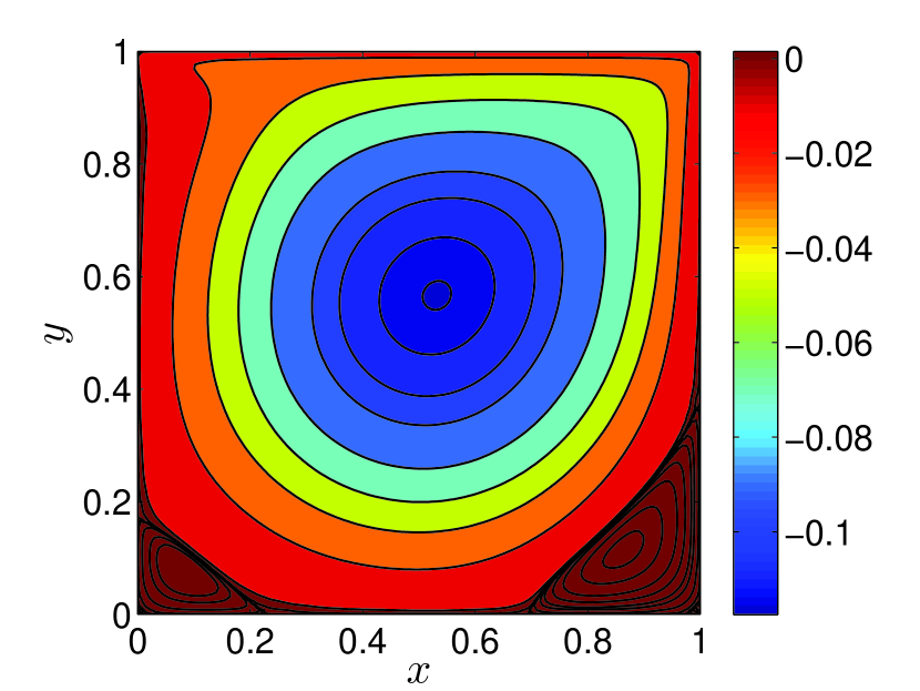
The streamline contours for the lid-driven cavity flow are shown in Figure 5. In 5(a), the full model matches well with the numerical results from [9], and the values of $\psi$ of the contours are the same as shown in Table III of [9]. Local SIRM provides an approximate solution. The main error occurs around the vortex center, where the contour of $\psi=-0.1175$ is missing in 5(b).

(a)

(b)

Figure 6: (a) Comparison of the velocity component $u(x=0.5,y)$ along the $y$-direction passing the geometric center between the full model, the coarse model, and the local SIRM method at $t=50$. (b) Comparison of the velocity component $v(x,y=0.5)$ along the $x$-direction passing geometric center between the full model, the coarse model, and the local SIRM method at $t=50$.

Figure 7: Comparison of the computational time of the full model and the local SIRM method for the lid-driven cavity flow problem. As the resolution increases from $65\times 65$ to $257\times 257$, the dimension of the full system, $n$, increases from $2\times 65^{2}$ to $2\times 257^{2}$. Using a log-log plot, the asymptotic complexity can be determined by the linear regression coefficient.

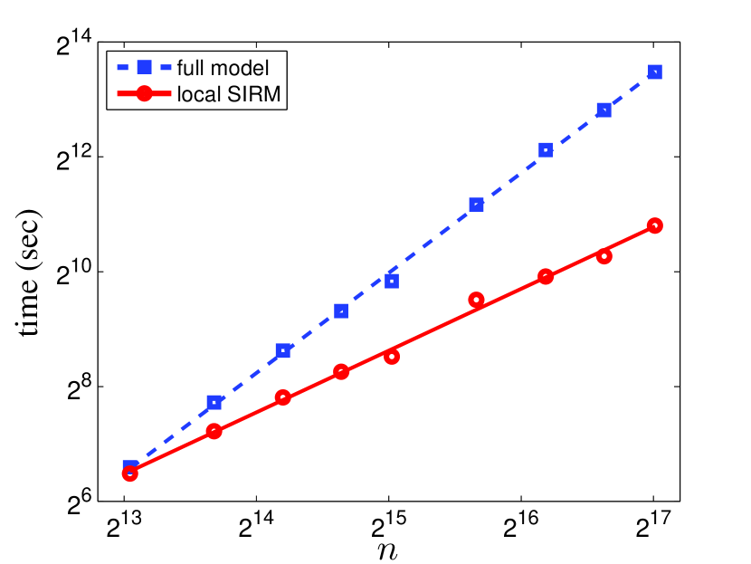
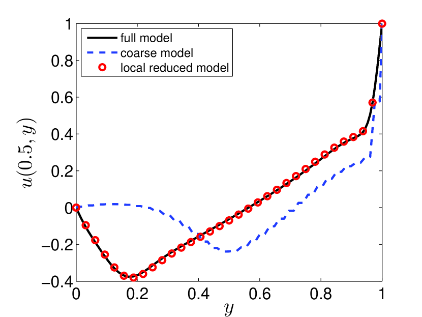
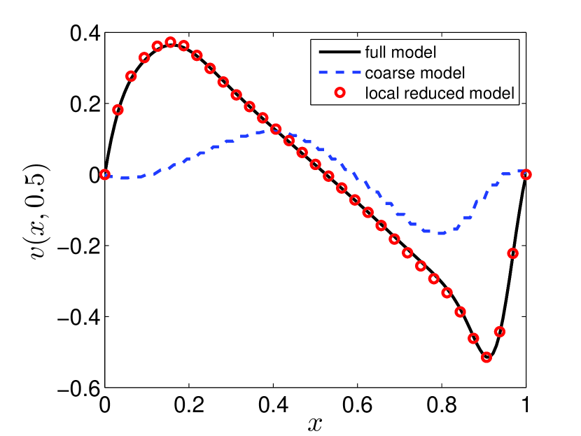
Figure 6 shows the velocity profiles for $u$ along the vertical line and $v$ along the horizontal line passing through the geometric center of the cavity. The coarse model provides a trial solution, which significantly deviates from the actual one. Then, local SIRM is used to obtain much more accurate results. For each iteration, three snapshots and their corresponding tangent vectors are used to form the information matrix. Instead of POD, the Gram–Schmidt process is applied here to form a set of orthonormal empirical eigenfunctions. Since the local data ensemble contains both $\psi$ and $\omega$ as well as the associated tangent vectors, the subspace dimension is $12$. An average of five iterations are carried out to obtain a local convergent solution for each subinterval.

Since an explicit scheme is used for the advection term, the CFL condition, $u\delta t/\delta x+v\delta t/\delta y\leq 1$ is a necessary condition for stability. Therefore, if the number of grid points increases from $65\times 65$ to $257\times 257$, the unit time step decreases from $10^{-2}$ to $2.5\times 10^{-3}$ accordingly. Accounting for this, the asymptotic computational complexity of the full model for the entire time domain is no less than $\mathcal{O}(n^{1.5})$. The above analysis only focuses on the advection term. Since the diffusion term uses an implicit scheme, there is no extra limit to the unit time step for the stability requirement. However, a large $n$ will lead to a slower convergence for many iterative methods, such as the successive over-relaxation method or the conjugate gradient method. Thus, $\mathcal{O}(n^{1.5})$ provides only a low bound estimation for the full model.

Since the Navier–Stokes equation contains only linear and quadratic terms, the complexity of the reduced model constructed by the Galerkin projection for one-step integration does not explicitly depend on $n$. Moreover, the computational complexity of all the other terms of local SIRM in Table 3 depends at most linearly on $n$. Thus, we may roughly estimate that the overall complexity of local SIRM is $\mathcal{O}(n)$. Figure 7 compares the running time of the full model and the running time of SIRM for different resolutions in (55) and (56). Except $n$ and $\delta t$, all the parameters remain the same. The linear regression indicates that the asymptotic complexity of the full model is $\mathcal{O}(n^{1.74})$, and the asymptotic complexity of the reduced model is $\mathcal{O}(n^{1.07})$ using the same scheme.

Table 4: The maximal $L_{2}$ error between the benchmark solution and approximate solutions solved by the local SIRM method for different $m$ and $m^{\prime}$ values.

	$m^{\prime}=2$	$m^{\prime}=3$	$m^{\prime}=5$	$m^{\prime}=6$	$m^{\prime}=10$
$m=500$	0.5689	0.5499	0.5407	0.5411	0.5403
$m=250(m^{\prime}-1)$	1.5029	0.5499	0.2335	0.1930	0.1175

Finally, Table 4 shows the maximal $L_{2}$ error for the local SIRM method using different $m$ and $m^{\prime}$ values. If each local reduced equation is solved in a larger subinterval with more modes while the total number of sampling snapshots remains the same, there is no significant improvement in accuracy. On the other hand, if the length of each subinterval remains the same but we sample more snapshots, a more accurate solution can be achieved. Thus, a good $m$ value should balance accuracy and cost of the reduced model, while a small $m^{\prime}$ is desired for the lid-driven cavity flow problem.

5 Conclusion

In this article, a new online manifold learning framework, subspace iteration using reduced models (SIRM), was proposed for the reduced-order modeling of large-scale nonlinear problems where both the data sets and the dynamics are systematically reduced. This framework does not require prior simulations or experiments to obtain state vectors. During each iteration cycle, an approximate solution is calculated in a low-dimensional subspace, providing many snapshots to construct an information matrix. The POD (SVD) method could be applied to generate a set of empirical eigenfunctions that span a new subspace. In an ideal case, a sequence of functions defined by SIRM uniformly converges to the actual solution of the original problem. This article also discussed the truncation error produced by SIRM and provided an error bound. The capability of SIRM to solve a high-dimensional system with high accuracy was demonstrated in several linear and nonlinear equations. Moreover, SIRM could also be used as a posterior error estimator for other coarse or reduced models.

In addition, the local SIRM method was developed as an extension that can reduce the cost of SIRM. The SIRM method is used to obtain a better approximate solution for each subinterval of a partitioned time domain. Because each subinterval has less state variation, the associated reduced model could be small enough. The numerical results of the nonlinear Navier–Stokes equation through a cavity flow problem implied that the local SIRM method could obtain significant speedups for a large-scale problem while maintaining good accuracy.

There are some interesting open questions to study in the future. For example, since the choice of the extended data ensemble is not unique, there might be other methods that can be used to form an information matrix that results in a more efficiently reduced model. It should be noted that the POD-Galerkin approach is not the only technique that can be used to extract the dominant modes from an information matrix and to construct a reduced model. How to combine SIRM with other model reduction techniques that exhibit higher efficiency remains a topic for future research.

References

- [1] D. Amsallem, M. J. Zahr, and C. Farhat, Nonlinear model order reduction based on local reduced-order bases, Int. J. Numer. Meth. Engng, 92 (2012), pp. 891–916.
- [2] A. C. Antoulas, Approximation of Large-Scale Dynamical Systems, SIAM, Philadelphia, PA, 2005.
- [3] A. C. Antoulas, D. C. Sorensen, and S. Gugercin, A survey of model reduction methods for large-scale systems, Contemp. Math., 280 (2001), pp. 193–219.
- [4] Z. Bai, Krylov subspace techniques for reduced-order modeling of large-scale dynamical systems, Appl. Numer. Math., 43 (2002), pp. 9–44.
- [5] S. Chaturantabut and D. C. Sorensen, Nonlinear model reduction via discrete empirical interpolation, SIAM J. Sci. Comput., 32 (2010), pp. 2737–2764.
- [6] Y. Chen and J. White, A quadratic method for nonlinear model order reduction, in Proc. Int. Conf. Modeling and Simulation of Microsystems, 2000, pp. 477–480.
- [7] M. Dihlmann, M. Drohmann, and B. Haasdonk, Model reduction of parametrized evolution problems using the reduced basis method with adaptive time partitioning, Technical Report 2011-13, Stuttgart Research Centre for Simulation Technology, Stuttgart, Germany, May 2011.
- [8] J. L. Eftang, A. T. Patera, and E. M. Rønquist, An “” certified reduced basis method for parametrized elliptic partial differential equations, SIAM J. Sci. Comput., 32 (2010), pp. 3170–3200.
- [9] U. Ghia, K. N. Ghia, and C. T. Shin, High-Re solutions for incompressible flow using the Navier–Stokes equations and a multigrid method, J. Comput. Phys., 48 (1982), pp. 387–411.
- [10] M. A. Grepl, Y. Maday, N. C. Nguyen, and A. T. Patera, Efficient reduced-basis treatment of nonaffine and nonlinear partial differential equations, M2AN Math. Model. Numer. Anal., 41 (2007), pp. 575–605.
- [11] P. Holmes, J. L. Lumley, G. Berkooz, and C. W. Rowley, Turbulence, Coherent Structures, Dynamical Systems and Symmetry, Cambridge Univ. Press, Cambridge, UK, 2nd ed., 2002.
- [12] S. Lall, J. E. Marsden, and S. Glavas̆ki, A subspace approach to balanced truncation for model reduction of nonlinear control systems, Int. J. Robust. Nonlinear Control, 12 (2002), pp. 519–535.
- [13] M. Loève, Probability Theory, Van Nostrand, Princeton, N.J., 1955.
- [14] R. Markovinović and J. D. Jansen, Accelerating iterative solution methods using reduced-order models as solution predictors, Int. J. Numer. Meth. Engng, 68 (2006), pp. 525–541.
- [15] J. D. Meiss, Differential Dynamical Systems, SIAM, Philadelphia, PA, 2007.
- [16] B. C. Moore, Principal component analysis in linear systems: Controllability, observability, and model reduction, IEEE Trans. Automat. Contr., 26 (1981), pp. 17–32.
- [17] M. L. Rapún and J. M. Vega, Reduced order models based on local POD plus Galerkin projection, J. Comput. Phys., 229 (2010), pp. 3046–3063.
- [18] M. Rathinam and L. R. Petzold, Dynamic iteration using reduced order models: A method for simulation of large scale modular systems, SIAM J. Numer. Anal., 40 (2002), pp. 1446–1474.
- [19] , A new look at proper orthogonal decomposition, SIAM J. Numer. Anal., 41 (2003), pp. 1893–1925.
- [20] M. Rewieński and J. White, A trajectory piecewise-linear approach to model order reduction and fast simulation of nonlinear circuits and micromachined devices, IEEE Trans. Comput. Aided Des. Integr. Circuits Syst., 22 (2003), pp. 155–170.
- [21] , Model order reduction for nonlinear dynamical systems based on trajectory piecewise-linear approximations, Linear Algebra Appl., 415 (2006), pp. 426–454.
- [22] D. Ryckelynck, A priori hyperreduction method: An adaptive approach, J. Comput. Phys., 202 (2005), pp. 346–366.
- [23] J. M. A. Scherpen, Balancing for nonlinear systems, Systems Control Letters, 21 (1993), pp. 143–153.
- [24] A. Thom, The flow past circular cylinders at low speed, Proc. Roy. Soc. Lond. A., 141 (1933), pp. 651–669.
- [25] L. N. Trefethen and D. Bau, Numerical Linear Algebra, SIAM, Philadelphia, PA, 1997.
- [26] D. S. Weile, E. Michielssen, and K. Gallivan, Reduced-order modeling of multiscreen frequency-selective surfaces using Krylov-based rational interpolation, IEEE Trans. Antennas Propag., 49 (2001), pp. 801–813.