A Study of Different Modeling Choices For Simulating Platelets Within the Immersed Boundary Method

Abstract

The Immersed Boundary (IB) method is a widely-used numerical methodology for the simulation of fluid-structure interaction problems. The IB method utilizes an Eulerian discretization for the fluid equations of motion while maintaining a Lagrangian representation of structural objects. Operators are defined for transmitting information (forces and velocities) between these two representations. Most IB simulations represent their structures with piecewise-linear approximations and utilize Hookean spring models to approximate structural forces. Our specific motivation is the modeling of platelets in hemodynamic flows. In this paper, we study two alternative representations – radial basis functions (RBFs) and Fourier-based (trigonometric polynomials and spherical harmonics) representations – for the modeling of platelets in two and three dimensions within the IB framework, and compare our results with the traditional piecewise-linear approximation methodology. For different representative shapes, we examine the geometric modeling errors (position and normal vectors), force computation errors, and computational cost and provide an engineering trade-off strategy for when and why one might select to employ these different representations.

1 Introduction

The Immersed Boundary (IB) Method was introduced by Charles Peskin in the early 1970’s to solve the coupled equations of motion of a viscous, incompressible fluid and one or more massless, elastic surfaces or objects immersed in the fluid [26]. Rather than generating a body-fitted grid for both exterior and interior regions of each surface at each timestep and using these to determine the fluid motion, Peskin instead employed a uniform Eulerian Cartesian grid over the entire domain and discretized the immersed boundaries by a set of points that are not constrained to lie on the grid. In Peskin’s work as well as many of the follow-on works, this set of points was connected via piecewise linear segments with Hookean spring models being used for approximating structural forces. Spreading and interpolation operations are then defined for transferring force and velocity information between the Lagrangian-defined structures and the Eulerian-discretized equations of motion.

The IB method was originally developed to model blood flow in the heart and through heart valves [26, 28, 29], but has since been used in a wide variety of other applications, particularly in biofluid dynamics problems where complex geometries and immersed elastic membranes or structures are present and make traditional computational approaches difficult. Examples include platelet aggregation in blood clotting [6, 10, 11], swimming of organisms [6, 7], biofilm processes [3], mechanical properties of cells [1], cochlear dynamics [2], and insect flight [22, 23].

We are motivated by the application of the IB method to platelet aggregation in blood clotting. Real platelets circulate with the blood in an inactive state in which they have a discoidal shape. In order to participate in clot formation, a platelet must undergo an activation process, one aspect of which is that the platelet changes shape and becomes more spherical. In IB modeling, inactive platelets are approximately elliptical or ellipsoidal in 2D and 3D, respectively, while activated platelets are approximately circular in 2D and spherical in 3D. Piecewise linear approximations of platelets are currently used within IB methods applied to platelet aggregation (e.g. [6, 10, 11]). We seek to explore alternative methods for the modeling of platelets that might decrease the computational time necessary to maintain and update platelet geometry and motion with comparable or better error characteristics to the standard piecewise linear models.

In this paper, we examine two alternative representations for platelets: interpolation with Fourier-based techniques (trigonometric polynomials in 2D and spherical harmonics in 3D) and interpolation with radial basis functions (restricted to the unit circle in 2D and unit sphere in 3D). Fourier methods have frequently been used for the modeling of circular and spherical objects (e.g. [31]). A recent result of Fornberg and Piret shows that both trigonometric polynomials and spherical harmonics are just special cases of radial basis functions (RBFs) when one chooses the shape parameter in a particular limit [13]. Additionally, error estimates for RBF interpolation on the circle and sphere have been given for a much wider range of target functions than just $C^{\infty}$ [19, 21, 24].

To perform a platelet IB computation, one must (1) have a representation of the surface of the platelet and (2) be able to compute forces (internal structural forces) at a specified collection of material points on the platelet surface. Once forces are determined, they are “projected” to an Eulerian mesh in which they are incorporated into the solution of the Navier-Stokes equations for determining the motion of the fluid. Based upon the updated fluid velocity field, the platelet’s position and shape are updated. We will not detail how the projection and interpolation are accomplished as this has been amply discussed in other works (e.g. [25]). Our focus is instead restricted to models for representing the platelet objects and how these can be used for constructing and maintaining the object’s representation, computing the normal vectors to the object, and computing the internal structural forces.

For results, we will compare the piecewise linear, Fourier, and RBF based methods for two different shapes in 2D and two different shapes in 3D that typify observed platelet geometries. We compare the errors in reconstructing these shapes, computing the normal vectors, and computing the forces. We provide a discussion of the engineering trade-offs we observe with respect to error and computational costs. Our results indicate that the RBF and Fourier models are viable alternatives to the piecewise linear models for platelet-like geometries in terms of errors versus computational cost. We furthermore find that the RBF models give better results for objects of varying smoothness than the Fourier models, and thus appear to be more promising in applications.

The paper is organized as follows. In Section 2 we present the three different modeling approaches: piecewise linear, Fourier, and RBFs. In Section 3 we review the components necessary for handling immersed elastic structures in the IB method. In Section 4 we provide implementation details for all three models in terms of computing normal vectors and forces for the platelets. Results are partitioned into two sections by spatial dimension. In Section 5 we present our comparison of the three modeling methodologies for 2D platelet objects, while in Section 6 we present our comparison for 3D platelet objects. Section 7 contains a summary of our findings.

2 Geometric Modeling Strategies

In this section we present the three different geometric modeling approaches to be examined. We first present the (traditional) piecewise linear approach for modeling two and three dimensional platelet structures. We then present our two alternative strategies based on a parametric representation of the surface: Fourier-based models (trigonometric series in 2D and spherical harmonic series in 3D) and radial basis function (RBF) models. Implementation details for all three methodologies are provided in Section 4.

2.1 Piecewise Linear Models

In the traditional (IB) method, parametric representations of the surface are rarely formed explicitly. Typically, a piecewise linear representation of the boundary is maintained. In 2D, the piecewise linear interpolant is a set of line segments between pairs of IB points. However, to perform secondary computations (such as computing normals) with a greater level of accuracy than what the piecewise linear interpolant would offer, piecewise quadratic interpolants are typically fitted to a set of IB points(e.g. [37, §3.1.1]).

Given a parameter $\lambda$, the piecewise quadratic representation is therefore defined as:

$$x(\lambda) \approx a_{x}{\lambda}^{2}+b_{x}{\lambda}+c_{x},$$ (1)

$$y(\lambda) \approx a_{y}{\lambda}^{2}+b_{y}{\lambda}+c_{y}.$$ (2)

The coefficients are computed by solving two linear systems of equations for each IB point; the right hand sides to these systems of equations are simply the x and y coordinates of the three IB points to which the piecewise quadratics are fitted to. Once the coefficients are obtained, one can now compute derivatives (and therefore normals and other quantities) at each IB point.

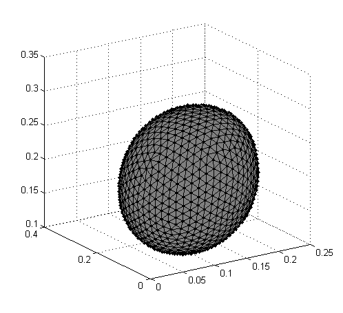
In 3D, the piecewise linear interpolant is a triangulation of the IB points (e.g. [11]). An example of such a triangulated surface is given in Figure 1. Secondary computations, such as computing normals and forces are computed from the triangulation as discussed in Section 4.1.

Figure 1: Illustration of the triangulation of a set of IB points in 3D.

2.2 Parametric models

The Fourier and RBF models we propose are both based on explicit parametric representations of the objects. Since our target objects are platelets, which in 2D models are nearly elliptical or circular and in 3D models are nearly ellipsoidal or spherical, we choose circular (or polar) and spherical parameterizations in 2D and 3D, respectively. Before discussing the two modeling approaches, we introduce some notation and put the modeling problem in the context of a reconstruction problem using interpolation.

In 2D, we use the following polar parametric notation to represent any of the objects:

$$\boldsymbol{x}(\lambda)=(x(\lambda),y(\lambda)),$$ (3)

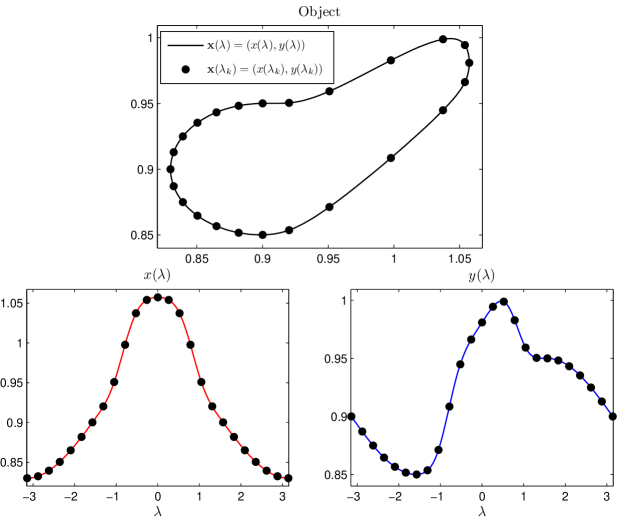
where $-\pi\leq\lambda\leq\pi$ and $\boldsymbol{x}(-\pi)=\boldsymbol{x}(\pi)$. In the case the object is a circle of radius $r$, $\boldsymbol{x}(\lambda)=(r\cos\lambda,r\sin\lambda)$. In general, given a finite collection of values of the object, $\{\boldsymbol{x}(\lambda_{k})\}_{k=1}^{N}$ = $\{(x(\lambda_{k}),y(\lambda_{k}))\}_{k=1}^{N}$, our goal is to reconstruct $\boldsymbol{x}(\lambda)$ from smooth interpolations of each of its components. We refer to these values as the data sites and the set of values $\{\lambda_{k}\}_{k=1}^{N}$ as the nodes. Figure 2 illustrates this reconstruction problem, of which the main ingredient is the interpolation of a function defined on the unit circle.

Figure 2: Illustration of the parametric representation of a 2D object $\boldsymbol{x}(\lambda)$ and the reconstruction from a finite number of data sites. The top figure shows the 2D object together with discrete data sites $\boldsymbol{x}(\lambda_{k})=(x_{k},y_{k})$. The bottom left figure shows the $x$ component of the object in parametric space and its values at the node set $\{\lambda_{k}\}_{k=1}^{N}$, while the right figure shows the $y$ component and its corresponding values. The goal is to reconstruct $x(\lambda)$ and $y(\lambda)$ from interpolations of these values at the node sets shown and then use these to reconstruct $\boldsymbol{x}(\lambda)$.

In 3D, we represent any of the objects using the following spherical parametric notation:

$$\boldsymbol{x}(\lambda,\theta)=(x(\lambda,\theta),y(\lambda,\theta),z(\lambda,\theta)),$$ (4)

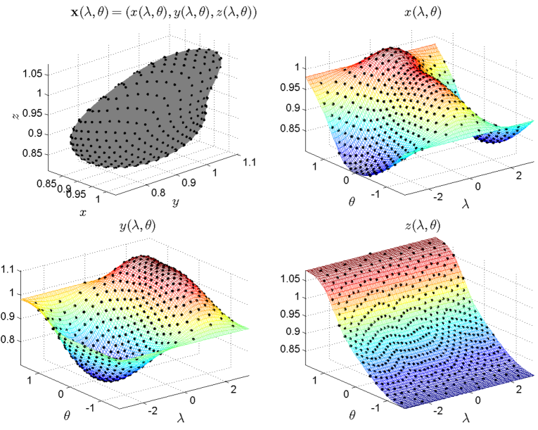
where $-\pi\leq\lambda\leq\pi$ and $-\pi/2\leq\theta\leq\pi/2$. Here the end conditions on $\boldsymbol{x}$ in $\lambda$ are $\boldsymbol{x}(-\pi,\theta)=\boldsymbol{x}(\pi,\theta)$, while the end conditions in $\theta$ are $\boldsymbol{x}(\lambda,\pi/2)=\boldsymbol{x}(\lambda+\pi,\pi/2)$ and $\boldsymbol{x}(\lambda,-\pi/2)=\boldsymbol{x}(\lambda+\pi,-\pi/2)$ for $-\pi\leq\lambda\leq 0$ and $\boldsymbol{x}(\lambda,\pi/2)=\boldsymbol{x}(\lambda-\pi,\pi/2)$ and $\boldsymbol{x}(\lambda,-\pi/2)=\boldsymbol{x}(\lambda-\pi,-\pi/2)$ for $0<\lambda\leq\pi$. These end conditions on $\theta$ are to enforce continuity of $\boldsymbol{x}$ at the poles of the spherical coordinate system. In the case the object is a sphere of radius $r$, $\boldsymbol{x}(\lambda,\theta)=(r\cos\lambda\cos\theta,r\sin\lambda\cos\theta,r\sin\theta)$. Similar to 2D, our goal is to reconstruct a general object $\boldsymbol{x}(\lambda,\theta)$ from smooth interpolations of each of its components which are given at some finite collection of locations $\{\boldsymbol{x}(\lambda_{k},\theta_{k})\}_{k=1}^{N}$ = $\{(x(\lambda_{k},\theta_{k}),y(\lambda_{k},\theta_{k}),z(\lambda_{k},\theta_{k}))\}_{k=1}^{N}$. We again refer to these values as the data sites and $\{(\lambda_{k},\theta_{k})\}_{k=1}^{N}$ as the nodes. Figure 3 illustrates this reconstruction problem, of which the main ingredient is the interpolation of a function defined on the unit sphere.

Figure 3: Illustration of the parametric representation of a 3D object $\boldsymbol{x}(\lambda,\theta)$ and the reconstruction from a finite number of data sites. Top left figure shows the 3D object together with discrete data sites $\{(x(\lambda_{k},\theta_{k}),y(\lambda_{k},\theta_{k}),z(\lambda_{k},\theta_{k})\}_{k=1}^{N}$ represented as black solid spheres. Top right figure shows the $x$ component of the object in spherical parametric space and its values at the node set $\{(\lambda_{k},\theta_{k})\}_{k=1}^{N}$ (marked by black solid spheres), while the bottom left and right figures show the respective $y$ and $z$ components and their corresponding values. The goal is to reconstruct $x(\lambda,\theta)$, $y(\lambda,\theta)$, and $z(\lambda,\theta)$ from interpolations of the values at the node sets shown and then use these to reconstruct $\boldsymbol{x}(\lambda,\theta)$.

2.2.1 Fourier Models

Since the modeling problems involve interpolation on the unit circle in 2D and the unit sphere in 3D, a natural choice for constructing these interpolants are Fourier based methods: trigonometric function for 2D objects and spherical harmonics for 3D objects. These methods have been used extensively for geometric modeling (see for example [31] and the references therein). We briefly review both of these interpolation techniques in the context of Figures 2 and 3.

Using the notation from Figure 2, we first discuss the case of reconstructing the $x(\lambda)$ component of $\boldsymbol{x}(\lambda)$. In the case that the number of nodes $N$ is even, we consider a trigonometric interpolant to this data of the form

$$p^{x}(\lambda)=c^{x}_{0}+\sum_{k=1}^{N/2}c^{x}_{2k-1}\cos k\lambda+\sum_{k=1}^{N/2-1}c^{x}_{2k}\sin k\lambda.$$ (5)

While there is an analogous formula for odd values of $N$, we omit this discussion and limit our current study to even values of $N$. The coefficients $c^{x}_{k}$ are determined by the interpolation conditions $p^{x}(\lambda_{k})=x(\lambda_{k})$, $k=1,\ldots,N$. The solution to this problem can be written in terms of the following linear system:

$$\begin{bmatrix}\vspace{0.1in}1&\cos\lambda_{1}&\sin\lambda_{1}&\cdots&\cos\dfrac{N-2}{2}\lambda_{1}&\sin\dfrac{N-2}{2}\lambda_{1}&\cos\dfrac{N}{2}\lambda_{1}\\ 1&\cos\lambda_{2}&\sin\lambda_{2}&\cdots&\cos\dfrac{N-2}{2}\lambda_{2}&\sin\dfrac{N-2}{2}\lambda_{2}&\cos\dfrac{N}{2}\lambda_{2}\\ \vdots&\vdots&\ddots&\vdots&\vdots&\vdots&\vdots\\ 1&\cos\lambda_{N}&\sin\lambda_{N}&\cdots&\cos\dfrac{N-2}{2}\lambda_{N}&\sin\dfrac{N-2}{2}\lambda_{N}&\cos\dfrac{N}{2}\lambda_{N}\end{bmatrix}\begin{bmatrix}c_{0}^{x}\vspace{0.1in}\\ c_{1}^{x}\vspace{0.1in}\\ \vdots\\ c_{N-1}^{x}\end{bmatrix}=\begin{bmatrix}x_{1}\vspace{0.1in}\\ x_{2}\vspace{0.1in}\\ \vdots\\ x_{N}\end{bmatrix},$$ (6)

where $x_{k}=x(\lambda_{k})$, $k=1,\ldots,N$. A similar construction to (5) is given for the $y(\lambda)$ component of $\boldsymbol{x}(\lambda)$, which we denote by $p^{y}(\lambda)$. Our trigonometric representation of a 2D object like the one in Figure 2 is given by

$${\boldsymbol{p}}(\lambda)=(p^{x}(\lambda),p^{y}(\lambda)).$$ (7)

We turn our attention now to interpolation with spherical harmonics and use the notation from Figure 3 to describe the reconstruction of the $x(\lambda,\theta)$ component of $\boldsymbol{x}(\lambda,\theta)$. The dimension of the space of all spherical harmonics of degree $M$ is given by $(M+1)^{2}$. For simplicity, we thus restrict our attention to the case that the number of nodes is given by $N=(M+1)^{2}$. In this case, we look for a spherical harmonic interpolant of the form

$$p^{x}(\lambda,\theta)=\sum_{\ell=0}^{M}\left[\sum_{m=0}^{\ell}c^{x}_{\ell,2m}Y_{\ell}^{2m}(\lambda,\theta)+\sum_{m=1}^{\ell}c^{x}_{\ell,2m-1}Y_{\ell}^{2m-1}(\lambda,\theta)\right],$$ (8)

where $Y_{\ell}^{2m}$ and $Y_{\ell}^{2m-1}$ are defined as follows:

$$Y_{\ell}^{2m}(\lambda,\theta) :=\sqrt{\frac{2\ell+1}{4\pi}\frac{(\ell-m)!}{(\ell+m)!}}\cos(m\lambda)P_{\ell}^{m}(\sin\theta),\quad m=0,\ldots,\ell,$$ (9)

$$Y_{\ell}^{2m-1}(\lambda,\theta) :=\sqrt{\frac{2\ell+1}{4\pi}\frac{(\ell-m)!}{(\ell+m)!}}\sin(m\lambda)P_{\ell}^{m}(\sin\theta),\quad m=1,\ldots,\ell.$$ (10)

Here $P_{\ell}^{m}$ is an associated Legendre function of degree $\ell$ and order $m$. The coefficients $c^{x}_{k}$ are determined by the interpolation conditions $p^{x}(\lambda_{k},\theta_{k})=x(\lambda_{k},\theta_{k})$, $k=1,\ldots,N$. The linear system corresponding to these conditions is given by

$$\begin{bmatrix}Y_{0}^{0}(\lambda_{1},\theta_{1})&Y_{1}^{0}(\lambda_{1},\theta_{1})&Y_{1}^{1}(\lambda_{1},\theta_{1})&Y_{1}^{2}(\lambda_{1},\theta_{1})&\cdots\\ Y_{0}^{0}(\lambda_{2},\theta_{2})&Y_{1}^{0}(\lambda_{2},\theta_{2})&Y_{1}^{1}(\lambda_{2},\theta_{2})&Y_{1}^{2}(\lambda_{2},\theta_{2})&\cdots\\ \vdots&\vdots&\vdots&\vdots&\vdots\\ Y_{0}^{0}(\lambda_{N},\theta_{N})&Y_{1}^{0}(\lambda_{N},\theta_{N})&Y_{1}^{1}(\lambda_{N},\theta_{N})&Y_{1}^{2}(\lambda_{N},\theta_{N})&\cdots\\ \end{bmatrix}\begin{bmatrix}c^{x}_{1}\\ c^{x}_{2}\\ \vdots\\ c^{x}_{N}\end{bmatrix}=\begin{bmatrix}x_{1}\\ x_{2}\\ \vdots\\ x_{N}\end{bmatrix},$$ (11)

where $x_{k}=x(\lambda_{k},\theta_{k})$, $k=1,\ldots,N$. Unlike the trigonometric case, this linear system can be singular depending on how the nodes are arranged [5, §2]. We avoid this possibility by choosing the nodes in an “optimal” manner as discussed in Section 4.2. For a good review of the properties of spherical harmonic interpolants see [35]. A similar construction to (8) is given for the $y(\lambda,\theta)$ and $z(\lambda,\theta)$ components of $\boldsymbol{x}(\lambda,\theta)$, which we denote by $p^{y}(\lambda,\theta)$ and $p^{z}(\lambda,\theta)$. Our spherical harmonic representation of a 3D object like the one in Figure 3 is given by

$${\boldsymbol{p}}(\lambda,\theta)=(p^{x}(\lambda,\theta),p^{y}(\lambda,\theta),p^{z}(\lambda,\theta)).$$ (12)

2.2.2 RBF Models

The RBF method is a popular tool for approximating multidimensional scattered data. An excellent overview of the theory and application of this method can be found in the two relatively recent books of Fasshauer [4] and Wendland [34]. The restriction of the RBF method to interpolation on a circle and on a sphere began to receive considerable attention from a theoretical standpoint starting in the mid 1990s (see [5, §6] for a discussion). When restricted to these domains, the RBF method is sometimes referred to as the zonal basis function (ZBF) or spherical basis function (SBF) method in the literature [34, Ch. 17]. We will, however, use the more popular term RBF to describe the interpolation technique. Several studies have been devoted to providing error estimates for RBF interpolation on circles and spheres; see, for example, [21, 24]. In the first of these papers, it is shown these interpolants can provide spectral accuracy provided the underlying target function is sufficiently smooth. The latter of these studies gives error estimates in the case that the target function belongs to some Sobolev space. Recently, the RBF method has been successfully used for approximating derivatives of scalar and vector-valued quantities on the surface of a sphere and incorporated into methods for solving partial differential equations numerically in spherical geometries [15, 8, 9].

The construction of the 2D and 3D RBF models of the objects is similar, so we discuss them together. Using the notation of Figures 2 and 3, and focusing on the reconstructions of the $x(\lambda)$ and $x(\lambda,\theta)$ components of the objects, the corresponding RBF interpolants are given by

$$\text{2D}: \quad s^{x}(\lambda) =\sum_{k=1}^{N}c^{x}_{k}\phi\left(\sqrt{2-2\cos(\lambda-\lambda_{k})}\right),$$ (13)

$$\text{3D}: \quad s^{x}(\lambda,\theta) =\sum_{k=1}^{N}c^{x}_{k}\phi\left(\sqrt{2(1-\cos\theta\cos\theta_{k}\cos(\lambda-\lambda_{k})-\sin\theta\sin\theta_{k})}\right).$$ (14)

Here $\phi$ is some scalar-valued, positive (semi-) definite radial kernel. The square root term in (13) is just the Euclidean distance between the points described in polar coordinates by $\lambda$ and $\lambda_{k}$, while the square root term in (14) is similarly the Euclidean distance between the points described in spherical coordinates by $(\lambda,\theta)$ and $(\lambda_{k},\theta_{k})$. The coefficients $c^{x}_{k}$ in either (13) or (14) are again determined by the interpolation conditions. These conditions lead to the following linear system of equations:

$$\underbrace{\begin{bmatrix}\phi\left(r_{1,1}\right)&\cdots&\phi\left(r_{1,N}\right)\\ \phi\left(r_{2,1}\right)&\cdots&\phi\left(r_{2,N}\right)\\ \vdots&\ddots&\vdots\\ \phi\left(r_{N,1}\right)&\cdots&\phi\left(r_{N,N}\right)\end{bmatrix}}_{\displaystyle A}\begin{bmatrix}c^{x}_{1}\\ c^{x}_{2}\\ \vdots\\ c^{x}_{N}\end{bmatrix}=\begin{bmatrix}x_{1}\\ x_{2}\\ \vdots\\ x_{N}\end{bmatrix},$$ (15)

where $x_{k}=x(\lambda_{k})$ and $r_{j,k}=\sqrt{2-2\cos(\lambda_{j}-\lambda_{k})}$ for 2D objects, and $x_{k}=x(\lambda_{k},\theta_{k})$ and $r_{j,k}$ $=\sqrt{2(1-\cos\theta_{j}\cos\theta_{k}\cos(\lambda_{j}-\lambda_{k})-\sin\theta_{j}\sin\theta_{k})}$ for 3D objects. Note that $r_{j,k}=r_{k,j}$ so that the linear system (15) is symmetric. More importantly, this linear system is guaranteed to be non-singular for the appropriate choice of $\phi$. In this study we restrict our attention to the multiquadric (MQ) and inverse multiquadric (IMQ) radial kernels, which are popular in applications and are given explicitly by

MQ: $$\phi(r)=\sqrt{1+(\varepsilon r)^{2}},$$ (16)

IMQ: $$\phi(r)=\dfrac{1}{\sqrt{1+(\varepsilon r)^{2}}}.$$ (17)

Here $\varepsilon$ is called the shape parameter. For both the MQ and IMQ, the linear system (15) is guaranteed to be non-singular (provided $\varepsilon>0$). Furthermore, for the IMQ, the $A$ matrix in this linear system is guaranteed to be positive definite. A full discussion of the non-singularity of (15) for various radial kernels can be found in either [4] or [34]. We postpone the discussion of choosing $\varepsilon$ to Section 4.3.2. We do, however, note that in the limit that $\varepsilon\rightarrow 0$ a RBF interpolant on a circle converges to a trigonometric interpolant, while a RBF interpolant on a sphere converges to a spherical harmonic interpolant [13] (strictly speaking this was only shown for the case of the sphere, but the arguments from [13] carry directly over to the case of the circle as well). Thus, trigonometric and spherical harmonic interpolation can be viewed as a special case of RBF interpolation.

We denote the RBF representations of a 2D object like the one in Figure 2 by

$${\boldsymbol{s}}(\lambda)=(s^{x}(\lambda),s^{y}(\lambda)),$$ (18)

where $s^{y}(\lambda)$ interpolates $y(\lambda)$ and has the form of (13). Similarly we denote the RBF representation of a 3D object like the one in Figure 3 by

$${\boldsymbol{s}}(\lambda,\theta)=(s^{x}(\lambda,\theta),s^{y}(\lambda,\theta),s^{z}(\lambda,\theta)),$$ (19)

where $s^{y}(\lambda,\theta)$ and $s^{z}(\lambda,\theta)$ interpolate $y(\lambda,\theta)$ and $z(\lambda,\theta)$, respectively, and have the form of (14).

We conclude this section by noting that the RBF method is more flexible than the Fourier-based methods in regard to altering the parameterization for the objects. For example, if one were to find that a more general ellipse or ellipsoid provided a better parameterization of the object than a circle or sphere, then the RBF method can be naturally extended to this new parameterization. The only change to (13) or (14) would be to replace the distance measure in the argument of $\phi$ with the appropriate (Euclidean) distance measure on the target object for the parametrization. More general objects, including ones with higher genus, are also possible; see [14] for a theoretical and numerical discussion.

3 Immersed Boundary Modeling

In this section we review the components needed for an immersed boundary model of platelets. Our focus here is on the computation of normal vectors and on the modeling of elasticity. For a discussion of how forces generated from immersed objects are transferred to the underlying Eulerian mesh and how the fluid velocity is updated see, for example,[25].

Normal vectors do not play a prominent role in most traditional IB calculations. Our interest in them is motivated by their other uses in the modeling of platelet aggregation. In addition to the fluid-structure interactions modeled using the IB method, the platelet problem requires solution of advection-diffusion equations for chemicals in the fluid domain outside of the moving platelets, along with boundary conditions on the chemical concentration at the fluid-platelet interface. Normal vectors along the platelet boundary are needed for determining when an Eulerian grid point is inside or outside of the platelet, and for imposing the boundary conditions. For further discussion of this, see [38].

3.1 Components for 2D

We denote the 2D platelet using the parametric representation $\boldsymbol{x}(\lambda)$ given in (3) and define

$$\boldsymbol{\tau}:=\frac{\partial}{\partial\lambda}\boldsymbol{x}(\lambda)=\left(\frac{\partial}{\partial\lambda}x(\lambda),\frac{\partial}{\partial\lambda}y(\lambda)\right)=(\boldsymbol{\tau}_{x},\boldsymbol{\tau}_{y}).$$ (20)

The unit tangent and normal vectors to $\boldsymbol{x}(\lambda)$ are then given as

$$\hat{\boldsymbol{\tau}}: =\frac{\boldsymbol{\tau}}{\|\boldsymbol{\tau}\|}=(\hat{\boldsymbol{\tau}}_{x},\hat{\boldsymbol{\tau}}_{y}),$$ (21)

$$\hat{\boldsymbol{\eta}}: =(-\hat{\boldsymbol{\tau}}_{y},\hat{\boldsymbol{\tau}}_{x})$$ (22)

For the force model in 2D, we use the fiber model defined in [27]. According to this model, the elastic force density on $\boldsymbol{x}(\lambda)$ at the location $\boldsymbol{x}(\lambda_{i})$ is given by

$$\mathbf{F}(\boldsymbol{x}(\lambda_{i}))=\left.\frac{\partial}{\partial\lambda}(T\hat{\boldsymbol{\tau}})\right|_{\lambda_{i}},$$ (23)

where $T=K(\|\boldsymbol{\tau}\|)$ is the fiber tension. In our platelet model, we choose $K$ as a linear function, $K=K_{0}\|\boldsymbol{\tau}\|$, where $K_{0}$ is the Hookean spring constant. In this case, (23) reduces to

$$\mathbf{F}(\boldsymbol{x}(\lambda_{i}))=K_{0}\left.\frac{\partial}{\partial\lambda}\left(\|\boldsymbol{\tau}\|\hat{\boldsymbol{\tau}}\right)\right|_{\lambda_{i}}=K_{0}\left.\frac{\partial^{2}}{\partial\lambda^{2}}\boldsymbol{x}(\lambda)\right|_{\lambda_{i}}.$$ (24)

The 2D spring force model traditionally used in piecewise linear representations is a scaled second-order, central-difference approximation to the above fiber model (assuming springs of zero rest length). From the physical standpoint, each IB point in a 2D object is thought to be connected to each of its neighbors via springs. For tension forces, there are only two neighbors attached to each IB point via springs. This spring force is expressed as:

$$\mathbf{F}(\boldsymbol{x}_{i})=K_{0}(\boldsymbol{x}_{i+1}-2\boldsymbol{x}_{i}+\boldsymbol{x}_{i-1}).$$ (25)

3.2 Components for 3D

We denote the 3D platelet using the parametric representation $\boldsymbol{x}(\lambda,\theta)$ given in (4) and define

$$\boldsymbol{\tau}^{\lambda}:= \frac{\partial}{\partial\lambda}\boldsymbol{x}(\lambda,\theta)=\left(\frac{\partial}{\partial\lambda}x(\lambda,\theta),\frac{\partial}{\partial\lambda}y(\lambda,\theta),\frac{\partial}{\partial\lambda}z(\lambda,\theta)\right),$$ (26)

$$\boldsymbol{\tau}^{\theta}:= \frac{\partial}{\partial\theta}\boldsymbol{x}(\lambda,\theta)=\left(\frac{\partial}{\partial\theta}x(\lambda,\theta),\frac{\partial}{\partial\theta}y(\lambda,\theta),\frac{\partial}{\partial\theta}z(\lambda,\theta)\right).$$ (27)

The unit tangent vectors to $\boldsymbol{x}(\lambda,\theta)$ are then given by

$$\hat{\boldsymbol{\tau}}^{\lambda}:=\frac{\boldsymbol{\tau}^{\lambda}}{\|\boldsymbol{\tau}^{\lambda}\|}\quad\text{and}\quad\hat{\boldsymbol{\tau}}^{\theta}:=\frac{\boldsymbol{\tau}^{\theta}}{\|\boldsymbol{\tau}^{\theta}\|},$$ (28)

while the unit normal vector is given by

$$\hat{\boldsymbol{\eta}}:=\frac{\boldsymbol{\tau}^{\lambda}\times\boldsymbol{\tau}^{\theta}}{\|\boldsymbol{\tau}^{\lambda}\times\boldsymbol{\tau}^{\theta}\|}.$$ (29)

The force model we use in 3D differs depending on whether a piecewise linear representation for the object is used or a parametric representation. Traditionally, piecewise linear representations (triangulated surfaces) in 3D have been used in conjunction with spring forces. In this model, a spring is assumed to be placed along each triangle edge (again, we assume these springs have a rest length of zero). Then, the total force acting on an IB point at $\boldsymbol{x}_{i}$ due to its $k$ nearest neighbors is:

$$\mathbf{F}(\boldsymbol{x}_{i})=K_{0}\sum_{j\neq i}(\boldsymbol{x}_{i}-\boldsymbol{x}_{j}),$$ (30)

where the sum is over $k$ IB points. The nearest neighbors are typically defined from the triangulation, i.e. as members of the adjacency list of $\boldsymbol{x}_{i}$. This is the same strategy that we follow.

For our parametric representation of platelets, we use surface tension as the model to compute tension forces. The force due to surface tension is then given by

$$\mathbf{F}=\gamma(2H)\hat{\boldsymbol{\eta}},$$ (31)

where $\gamma$ is the coefficient of surface tension. $H$ is the mean curvature of the surface, and can be computed as [17, §16.5]

$$H=\frac{eG-2fF+gE}{2(EG-F^{2})},$$ (32)

where $E$, $F$, and $G$ are coefficients of the first fundamental form,

$$E=\boldsymbol{\tau}^{\lambda}\cdot\boldsymbol{\tau}^{\lambda},\;F=\boldsymbol{\tau}^{\lambda}\cdot\boldsymbol{\tau}^{\theta},\;G=\boldsymbol{\tau}^{\theta}\cdot\boldsymbol{\tau}^{\theta},$$ (33)

and $e$, $f$, and $g$ are coefficients of the second fundamental form,

$$e=\left(\frac{\partial}{\partial\lambda}\boldsymbol{\tau}^{\lambda}\right)\cdot\hat{\boldsymbol{\eta}},\;f=\left(\frac{\partial}{\partial\theta}\boldsymbol{\tau}^{\lambda}\right)\cdot\hat{\boldsymbol{\eta}},\;g=\left(\frac{\partial}{\partial\theta}\boldsymbol{\tau}^{\theta}\right)\cdot\hat{\boldsymbol{\eta}}.$$ (34)

4 Implementation Details

In this section we present the implementation details for evaluating the positions on the Lagrangian objects, computing normals to the surface of the object, and computing the internal forces as presented in the previous section. For the piecewise linear representation, these surface normals and forces are computed at the IB points. For the parametric representations using Fourier and RBF models, these values are computed at some set of sample sites, which do not necessarily correspond to the data sites. With these operations defined, it is possible to employ the traditional spreading and interpolation operators for transferring the forces and velocity respectively between the Lagrangian and Eulerian discretizations.

4.1 Piecewise Linear Models

In 2D, normals are computed at the IB points using the piecewise quadratic representation presented in Section 2.1. For each IB point, we first solve for the coefficients in (1) and (2) using the IB point and its two neighbors. Using (1) and (2), we next compute the tangent vector at each IB point using (21) and then determine the normal vector using (22).

In 3D, we compute the normal vectors at each IB point by first computing the normal vector at the circumcenter of each of the triangles. We then obtain the normal vector at a vertex (IB point) by a weighted average of the values of the normal vectors at the circumcenters of the triangles connected to the vertex. Specifically, we weight these facet normals by the angle at which that facet is incident on the vertex at which we require a normal. This approach takes into account the geometric configuration of each facet [32].

The implementation of the forces follows directly from the simple spring force model in both 2D (25) and 3D (30). We note that while the 2D implementation follows naturally from a constitutive model, the 3D implementation is a purely algorithmic extension of the 2D case.

4.2 Parametric Models

For the parametric models, we use the continuous representations of the objects from either the Fourier or RBF based interpolants to approximate the normal vectors and forces. This involves analytically computing derivatives of these interpolants and then evaluating the derivatives at some set of $M$ locations in the parametric space that corresponds to the set of sample sites. In 2D, we denote the set of sample sites by $\{\boldsymbol{x}(\lambda^{\rm e}_{j})\}_{j=1}^{M}$ and refer to the set of parametric values $\{\lambda^{\rm e}_{j}\}_{j=1}^{M}$ as the evaluation points. Similarly for 3D, we denote the sample sites by $\{\boldsymbol{x}(\lambda^{\rm e}_{j},\theta^{\rm e}_{j})\}_{j=1}^{M}$ and refer to $\{(\lambda^{\rm e}_{j},\theta^{\rm e}_{j})\}_{j=1}^{M}$ as the evaluation points. The method we use is similar to the pseudospectral or spectral collocation method (e.g. [12, 33]), except that the derivatives are not evaluated at interpolation nodes.

Before describing the implementation details for the Fourier and RBF models, we discuss the node and evaluation points used.

4.3 Node and Evaluation points

For our 2D objects, we use $N$ equally-spaced points on the interval $(-\pi,\pi]$ as the node set $\{\lambda_{k}\}_{k=1}^{N}$, and take $N$ to be even. This gives a uniform sampling in the parametric space and allows fast algorithms to be used for computing the interpolants as discussed below. Additionally, since the shape of our target objects are near circular or elliptical, these nodes give a good distribution of data sites on the object. We also use $M>>N$ equally-spaced points in the interval $(-\pi,\pi]$ as the set of evaluation points $\{\lambda^{\rm e}_{j}\}_{j=1}^{M}$ since this also results in a set of sample sites that are well distributed over the object.

To get a good sampling of our nearly ellipsoidal or spherical objects in 3D, we cannot resort to using equally spaced points in the spherical coordinate system as our node sets $\{(\lambda_{k},\theta_{k})\}_{k=1}^{N}$ because of the inherent “pole problem”. Instead we use node sets that give a quasi-uniform distribution of data sites on the unit sphere. Since only a maximum of 20 points can be evenly distributed on a sphere, there are a myriad of methods to define and generate a quasi-uniform distribution for larger numbers of points [18]. We use two of these methods: maximal determinant (MD) for our spherical harmonic models and minimal energy (ME) for our RBF models. Both of these methods are discussed in [35] and many of these two point sets for various $N$ can be downloaded from [36]. The MD points are generated by finding a distribution of points that maximize the determinant of a certain “Gram matrix” related to (11). The ME points are generated by finding a distribution of nodes that minimize an electrostatic type energy potential. For spherical harmonic interpolation, the MD points lead to much better results both in terms of accuracy and stability [35]. For RBF interpolation, the ME points typically yield better results in terms of accuracy [8, 9] for larger shape parameters $\varepsilon$. For smaller values, the MD points give better results because of the connection to spherical harmonics as $\varepsilon\rightarrow 0$ [13]. For the set of evaluation points, $\{(\lambda^{\rm e}_{j},\theta^{\rm e}_{j})\}_{j=1}^{M}$, we use $M>>N$ ME points for both the spherical harmonic and RBF models, which again results in a well distributed set of sample sites on the object.

4.3.1 Fourier Models

The first step in computing the normal vectors and forces for the 2D trigonometric model (7) is to compute the interpolation coefficients $c_{k}^{x}$ and $c_{k}^{y}$, $k=1,\ldots,N$ (see (5)). Since we are using equally spaced node points $\{\lambda_{k}\}_{k=1}^{N}$, we can avoid having to solve (6) directly for these coefficients and can instead compute them by means of the fast Fourier transforms (e.g. [33, §3]) at a cost of $O(N\log N)$.

We next compute the derivatives of the interpolants to obtain the following approximation to (20):

$$\frac{\partial}{\partial\lambda}\boldsymbol{x}(\lambda)\bigr{|}_{\lambda=\lambda^{\rm e}_{j}}\approx\frac{\partial}{\partial\lambda}{\boldsymbol{p}}(\lambda)\bigr{|}_{\lambda=\lambda^{\rm e}_{j}},\;j=1,\ldots,M.$$ (36)

We then determine the normal vector at $\boldsymbol{x}(\lambda^{\rm e}_{j})$ by normalizing the vector above and switching the components according to (21) and (22). We similarly obtain an approximation of the force (24) from the second derivative of the interpolants:

$$\frac{\partial^{2}}{\partial\lambda^{2}}\boldsymbol{x}(\lambda)\bigr{|}_{\lambda=\lambda^{\rm e}_{j}}\approx\frac{\partial^{2}}{\partial\lambda^{2}}{\boldsymbol{p}}(\lambda)\bigr{|}_{\lambda=\lambda^{\rm e}_{j}},\;j=1,\ldots,M.$$ (37)

For the 3D spherical harmonic model (12), the first step in computing the normal vectors and forces is again to compute the interpolation coefficients $c_{k}^{x}$, $c_{k}^{y}$, and $c_{k}^{z}$, $k=1,\ldots,N$, (see (8)). Unlike the trigonometric interpolant, there are unfortunately no fast algorithms for computing these coefficients. Since we use relatively small values of $N$, we thus resort to determining the coefficients by solving the linear system (11) using a direct $LU$ factorization of the interpolation matrix. By using the MD points as the nodes in this model, we are guaranteed that this system is non-singular and relatively well conditioned [35]. We note that in context of the IB method simulation, the node points will stay fixed throughout the simulation so that the $LU$ factorization of the interpolation matrix from (11) needs to be done only once at the initial time-step and then stored. Thus, for all other time-steps the coefficients can be determined in $O(N^{2})$ computations.

After the coefficients are determined, we compute the following six derivatives to obtain approximations to (26) and (27):

$$\frac{\partial}{\partial\lambda}\boldsymbol{x}(\lambda,\theta)\bigr{|}_{(\lambda,\theta)=(\lambda^{\rm e}_{j},\theta^{\rm e}_{j})} \approx\frac{\partial}{\partial\lambda}{\boldsymbol{p}}(\lambda,\theta)\bigr{|}_{(\lambda,\theta)=(\lambda^{\rm e}_{j},\theta^{\rm e}_{j})},\;j=1,\ldots,M,$$ (38)

$$\frac{\partial}{\partial\theta}\boldsymbol{x}(\lambda,\theta)\bigr{|}_{(\lambda,\theta)=(\lambda^{\rm e}_{j},\theta^{\rm e}_{j})} \approx\frac{\partial}{\partial\theta}{\boldsymbol{p}}(\lambda,\theta)\bigr{|}_{(\lambda,\theta)=(\lambda^{\rm e}_{j},\theta^{\rm e}_{j})},\;j=1,\ldots,M.$$ (39)

We then compute the normal vectors using these approximations in (28) and (29).

The computation of the force requires the approximation to the normal vectors and an approximation to the mean curvature (32). For the values of $E$, $F$, and $G$ in the mean curvature computation (see (33)), we use the approximations (38) and (39). For the values of $e$, $f$, and $g$, we use the approximations

$$\frac{\partial^{2}}{\partial\lambda^{2}}\boldsymbol{x}(\lambda,\theta)\bigr{|}_{(\lambda,\theta)=(\lambda^{\rm e}_{j},\theta^{\rm e}_{j})} \approx\frac{\partial^{2}}{\partial\lambda^{2}}{\boldsymbol{p}}(\lambda,\theta)\bigr{|}_{(\lambda,\theta)=(\lambda^{\rm e}_{j},\theta^{\rm e}_{j})},\;j=1,\ldots,M,$$ (40)

$$\frac{\partial^{2}}{\partial\theta\partial\lambda}\boldsymbol{x}(\lambda,\theta)\bigr{|}_{(\lambda,\theta)=(\lambda^{\rm e}_{j},\theta^{\rm e}_{j})} \approx\frac{\partial^{2}}{\partial\theta\partial\lambda}{\boldsymbol{p}}(\lambda,\theta)\bigr{|}_{(\lambda,\theta)=(\lambda^{\rm e}_{j},\theta^{\rm e}_{j})},\;j=1,\ldots,M,$$ (41)

$$\frac{\partial^{2}}{\partial\theta^{2}}\boldsymbol{x}(\lambda,\theta)\bigr{|}_{(\lambda,\theta)=(\lambda^{\rm e}_{j},\theta^{\rm e}_{j})} \approx\frac{\partial^{2}}{\partial\theta^{2}}{\boldsymbol{p}}(\lambda,\theta)\bigr{|}_{(\lambda,\theta)=(\lambda^{\rm e}_{j},\theta^{\rm e}_{j})},\;j=1,\ldots,M.$$ (42)

4.3.2 RBF Models

The normal vectors and forces for the RBF models are computed in the same fashion as for the Fourier models discussed above; one just needs to replace the Fourier interpolants ${\boldsymbol{p}}(\lambda)$ and ${\boldsymbol{p}}(\lambda,\theta)$ with the RBF interpolants ${\boldsymbol{s}}(\lambda)$ from (18) and ${\boldsymbol{s}}(\lambda,\theta)$ from (19), respectively. We thus omit a full description. We will, however, discuss the shape parameter $\varepsilon$ and the computation of the interpolation coefficients.

Infinitely smooth radial kernels like the MQ (16) and IMQ (17) feature a free shape parameter $\varepsilon$. It has generally been reported in the literature that there is typically an optimal value of $\varepsilon$ that produces the best accuracy in the interpolants with these kernels and that this value tends to decrease with increasing smoothness of the underlying function being approximated (e.g. [30]). However, as $\varepsilon$ decreases to zero these smooth kernels become increasingly flat and the shifts of $\phi$ in (13) and (14) become less and less distinguishable from one another. If one follows the direct approach of solving for the expansion coefficients via (15) and then evaluating the interpolant via (13) or (14) (which is denoted by RBF-Direct in the current literature) for $\varepsilon$ in this flat regime, then ill-conditioning can entirely contaminate the computation. For RBF interpolation on a sphere, this ill-conditioning can be completely bypassed by replacing the RBF-Direct algorithm with the RBF-QR algorithm of Fornberg and Piret [13]. The framework for this algorithm can also naturally be adapted to the task of computing RBF interpolants on the unit circle in a stable manner for all $\varepsilon$.

We have implemented both the RBF-QR algorithm and the RBF-Direct approach and present results in Sections 5.2.1 and 6.2.1 illustrating the behavior of the RBF interpolants for the full range of $\varepsilon$ and the connection to Fourier based methods. However, we have opted to use the RBF-Direct approach in implementation since it is computationally more efficient and the coding is much less involved for computing the normals and forces. Additionally, we have found that with the RBF-Direct approach and the values of $N$ that we considered it is possible to get as good or better results than the Fourier based methods. For increasingly large values of $N$, or objects whose parameterizations are very smooth, it may be necessary to switch to the RBF-QR algorithms to exploit the better accuracy that can sometimes be achieved for increasingly small values of $\varepsilon$.

For the RBF-Direct approach, the interpolation coefficients for both the 2D and 3D objects can be determined by solving the linear system (15) (with the appropriate choice of $r_{j,k}$ for the dimension of interest). In the case of 2D objects with equally spaced points, solving this system directly can be bypassed by means of the fast Fourier transform and the coefficients can be computed in $O(N\log N)$ operations [20]. This follows by observing that the matrix in (15) is circulant (for any radial kernel $\phi$) and can be diagonalized via the discrete Fourier transform matrix [16, §4.7.7]. For the 2D models, we use the MQ radial kernel (16).

As in the case of the spherical harmonic model, there are no fast direct algorithms for determining the interpolation coefficients for the 3D RBF model (19) and we thus resort to using a direct method. However, unlike the spherical harmonic model the system is symmetric and, as discussed in Section 2.2.2, for the right choice of $\phi$ it is positive definite. Thus, a Cholesky factorization of the matrix can be used which reduces the memory costs and the need for pivoting over the $LU$ factorization method used in the spherical harmonic model. We also note that the initial cost of computing the Cholesky factorization is lower than the $LU$ factorization, but since this is only done once initially there is no real savings in an IB simulation. We have opted to use the IMQ kernel (16) to exploit the use of the Cholesky factorization.

5 2D Platelet Modeling Results

In this section, we present the results of our comparative study between using the piecewise linear approach as traditionally used within the IB method and our two alternative parametric approaches in 2D: RBF and Fourier (trigonometric polynomials) interpolation. Recall that within an IB timestep, the typical procedure employed is as follows. Given the locations of the immersed boundaries, both the normals and forces on an object are computed. The forces are then projected to an Eulerian grid and used as right-hand-side forcing to the Navier-Stokes equations. Based upon an update velocity field, the positions of the IB points are updated. In our comparison, we thus examine the geometric modeling capabilities, accuracy of the normal computations, and accuracy of the computation of the forces. As discussed in the previous section, we distinguish between the data sites and sample sites for the parametric models. Data sites are the positions along the object at which the parametric models are interpolating. It is at these positions that we propose updating the geometric information of the object (for instance, at the conclusion of a timestep when the object’s movement within the flow field is updated). Sample sites (which are normally more numerous compared to the data sites) are the positions along the object at which normals and forces are computed. It is from these positions that we propose projecting the IB forces. In all experiments, $100$ sample sites are used as this represents the typical number of IB points that would be used per platelet object in a traditional 2D immersed boundary computation (and hence a reasonable standard against which to compare our new methods for the purposes of determining the feasibility of replacement). All errors are computed by taking the maximum of the two-norm difference between the approximations and the true values.

5.1 Test Cases

We consider 2 prototypical test objects and define them based upon perturbations of idealized shapes (an ellipse and a circle). Let $\textbf{x}_{ideal}$ be a function representing the idealized, unperturbed shapes as given by the following equation:

$$\boldsymbol{x}_{ideal}=(x_{c}+a\cos\lambda,y_{c}+b\sin\lambda)$$ (43)

where $-\pi\leq\lambda\leq\pi$. Here $(x_{c},y_{c})$ denotes the object center and $a$ and $b$ denote the radii. The two objects used for our comparison are defined as follows:

$$\text{\text@underline{Object 1}:}\quad\boldsymbol{x}_{2d\,obj1} = \left[1.0+A\exp\left(\frac{-(1-\cos\lambda)^{2}}{\sigma_{1}}\right)\right]\,\boldsymbol{x}_{ideal},$$ (44)

$$\text{\text@underline{Object 2}:}\quad\boldsymbol{x}_{2d\,obj2} = \left[1.0+B\exp\left(\frac{(-(1-\cos^{2}\lambda)^{1.5})}{\sigma_{2}}\right)\right]\,\boldsymbol{x}_{ideal}.$$ (45)

For Object 1, we use the following parameters: $x_{c}=y_{c}=0.9$, $a=0.04$, $b=0.05$, $A=0.09$ and $\sigma_{1}=0.1$. For Object 2, we use the following parameters: $x_{c}=y_{c}=0.2$, $a=b=0.1$, $B=0.04$ and $\sigma_{2}=0.9$.

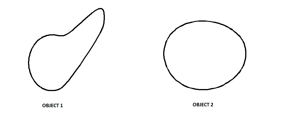
Figure 4 displays the two test objects (44) and (45). Object 1 is a smooth (in terms of regularity) yet highly perturbed ellipse, while Object 2 is a non-smooth perturbation of a circle. It can be shown that the parameterization (45) for this object has only two continuous derivatives.

Figure 4: The test objects (44) and (45) for the 2D study.

5.2 Comparison of Reconstructing the Objects

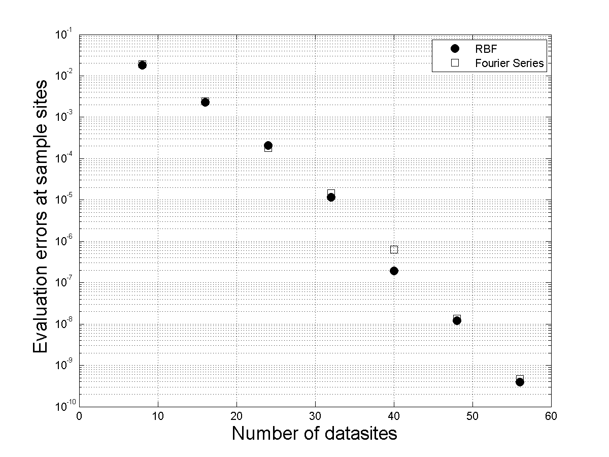
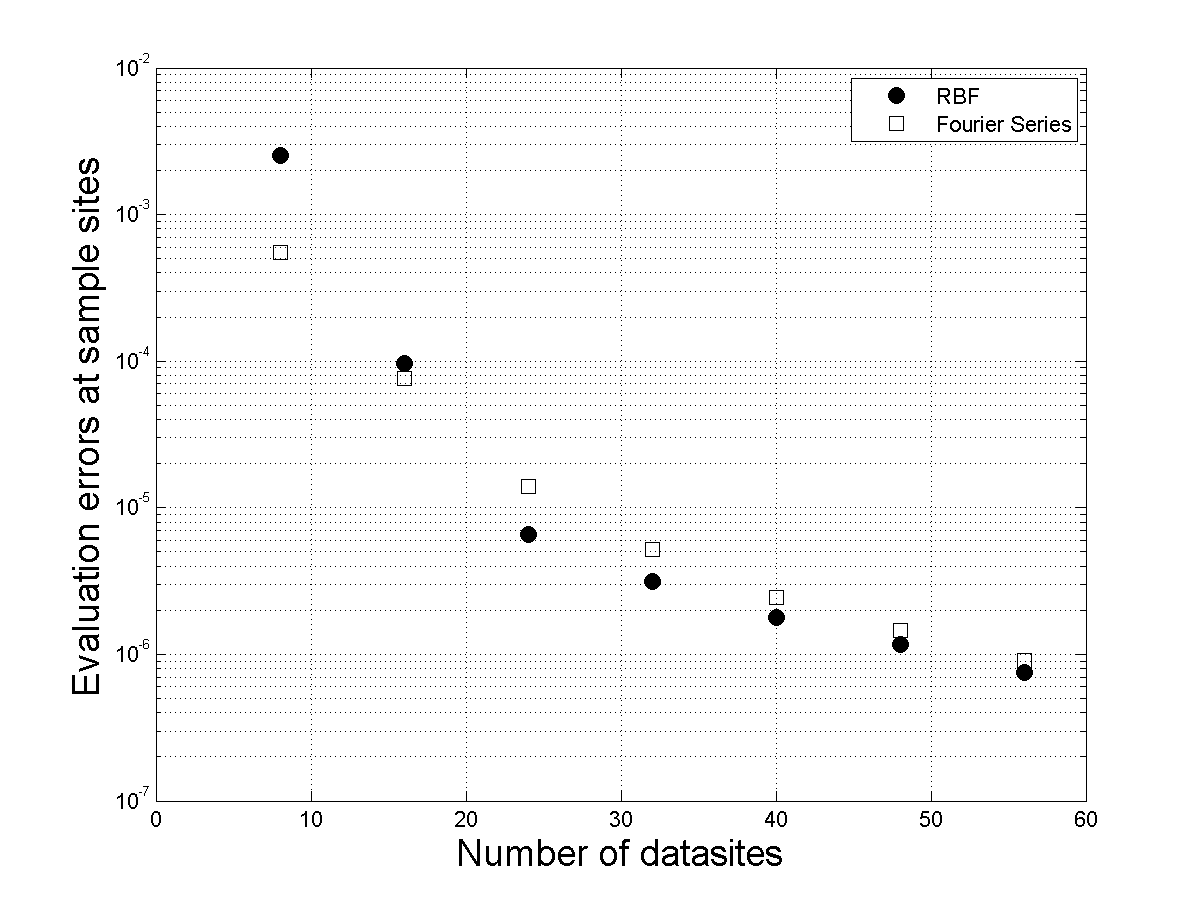
We first examine the errors in reconstructing the objects using the RBF and Fourier approaches. In Figure 5 we present the errors in reconstructing the objects as a function of the number of data sites. The error at the sample sites gives an indication of the modeling capability of the RBF and Fourier methods. We can see from this figure that both the RBF and Fourier models are converging at a spectral rate for Object 1 (left figure), but at a much slower rate for Object 2 (right figure). This is expected since Object 1 is infinitely smooth, while Object 2 has only two continuous derivatives. The RBF and Fourier models perform similarly for Object 1. For Object 2, the RBF model shows better reconstruction properties as the number of sample sites increases above 20. No direct comparison with the piecewise linear model is given as the piecewise linear IB method always samples at the interpolating points.

Figure 5: Error in the reconstruction of the shape of the objects (left is Object 1 and right is Object 2) evaluated at $M=100$ sample sites as a function of the number of data sites. Circles denote the errors in the RBF model and squares denote the errors for the Fourier model. For the RBF model, the shape parameter for Object 1 was set to $\varepsilon=0.9$ and for Object 2, it was set to $\varepsilon=3.6$.

5.2.1 Shape Parameter Study

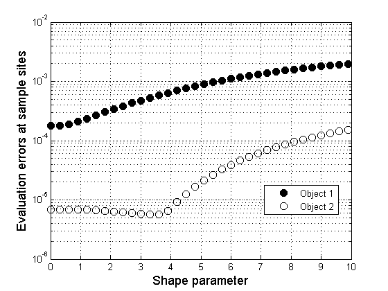
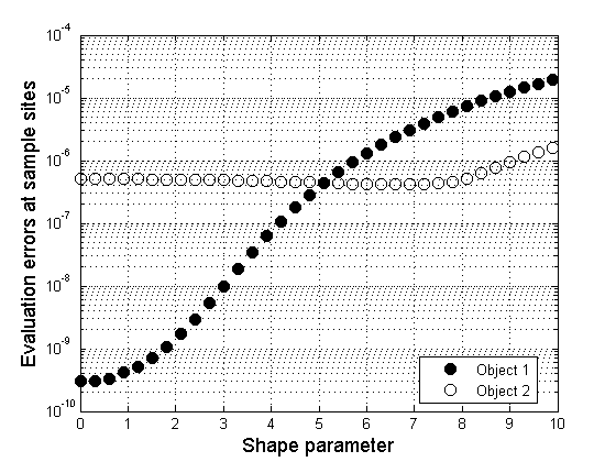
In this section, we examine the impact of the shape parameter on the reconstruction errors of the RBF model. Figure 6 displays the reconstruction errors for the two objects as a function of the shape parameter using $N=24$ data sites. A similar comparison for $N=56$ data sites is given in Figure 7. For $\varepsilon\lesssim 0.85$, it was necessary to use the RBF-QR algorithm [13] (adapted to the unit circle) to compute the model in a numerically stable manner for the $N=56$ case. We can see from both figures that the errors are smallest for $\varepsilon\approx 0$ for the smooth Object 1 and increase quite dramatically as $\varepsilon$ increases. For the non-smooth Object 2, there is a much larger range of $\varepsilon$ for which the errors are small, and this range includes values for which the RBF-Direct approach can be used without issues of numerical instabilities.

Figure 6: Errors in the RBF reconstructions of the objects using $N=24$ data sites and $M=100$ sample sites as a function of the shape parameter.

Figure 7: Errors in the RBF reconstructions of the objects using $N=56$ data sites and $M=100$ sample sites as a function of the shape parameter.

We used Figures 6 and 7 to help guide our selection of $\varepsilon$ for the numerical experiments. However, we found from extensive tests on other objects, that if the object is smooth, and RBF-Direct is to be used, then one generally wants to choose $\varepsilon$ as small as the numerical conditioning allows. For non-smooth objects there is much more freedom in the choice and the results will not vary that greatly. It is unclear if we should expect smooth or non-smooth objects in an IB simulation.

We conclude this section by noting that there are several algorithms that have been devoted to selecting an “optimal” shape parameter [4, §17]. However, these are too costly to be used every time-step of an IB simulation. We are thus advocating using a fixed $\varepsilon$ for all time-steps. This value could be selected based on an expected typical shape for the immersed objects and one of the algorithms from [4, §17] or from trial and error. We will report on these strategies in a follow up paper where the RBF models are used in actual IB method simulations.

5.3 Comparison of Normal Vectors and Forces

We next focus on the errors in the parametric models in the approximation of the normal vectors to the objects and the forces. In this case, we compare the results to the traditional piecewise linear models.

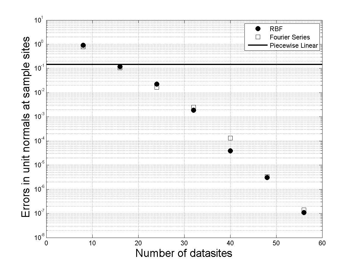
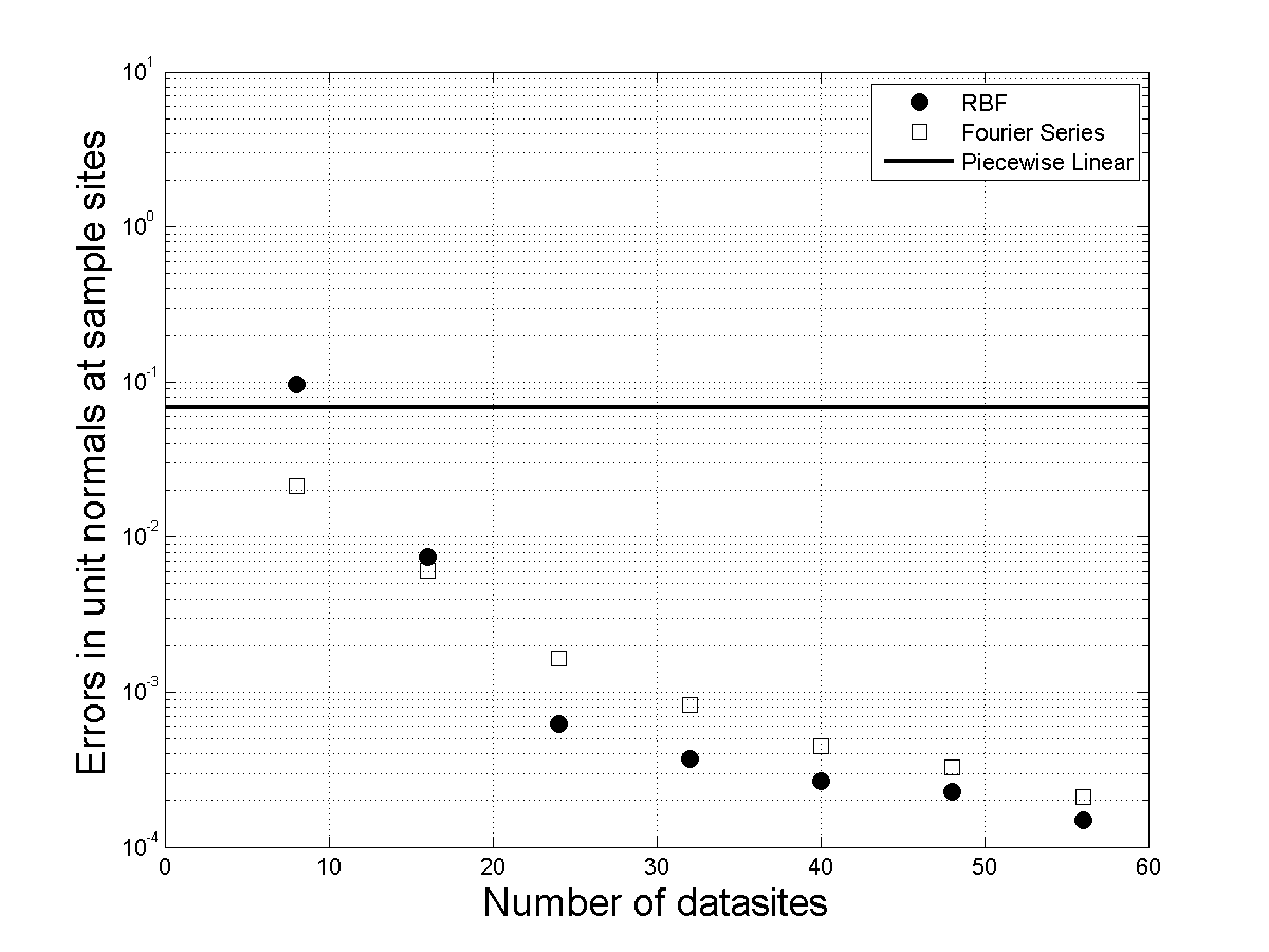
Figure 8 displays the errors in the normal vectors at $M=100$ sample sites as a function of the number of data sites $N$ for both the RBF and Fourier models. A solid line denoting the errors in the normal vectors for $100$ IB points is given for comparison using the method for the piecewise linear models discussed in Section 4.1. We can see from this figure that at about $N=18$ data sites the errors for both the RBF and Fourier models of Object 1 are lower than the piecewise linear model. The errors are similar between both parametric models and decrease rapidly with increasing $N$. The results for Object 2 are even more favorable for the parametric models compared to the piecewise linear model. For increasing $N$ the RBF model appears to have an advantage over the Fourier model.

Figure 8: Errors in the approximations of the normal vectors to the objects at $100$ sample sites as a function of the number of data sites $N$. The left plot is for Object 1, while the right one is for Object 2. The line denotes the error for the method used in the piecewise linear model with $100$ IB points. Circles denote the errors for the RBF model and squares denote the Fourier model. For the RBF model, $\varepsilon=0.9$ for Object 1 and $\varepsilon=3.6$ for Object 2.

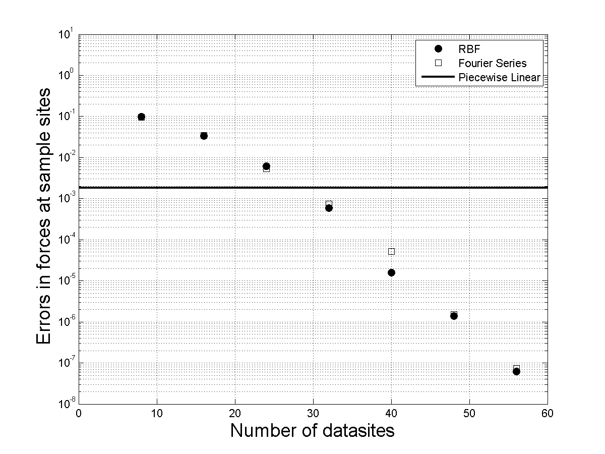
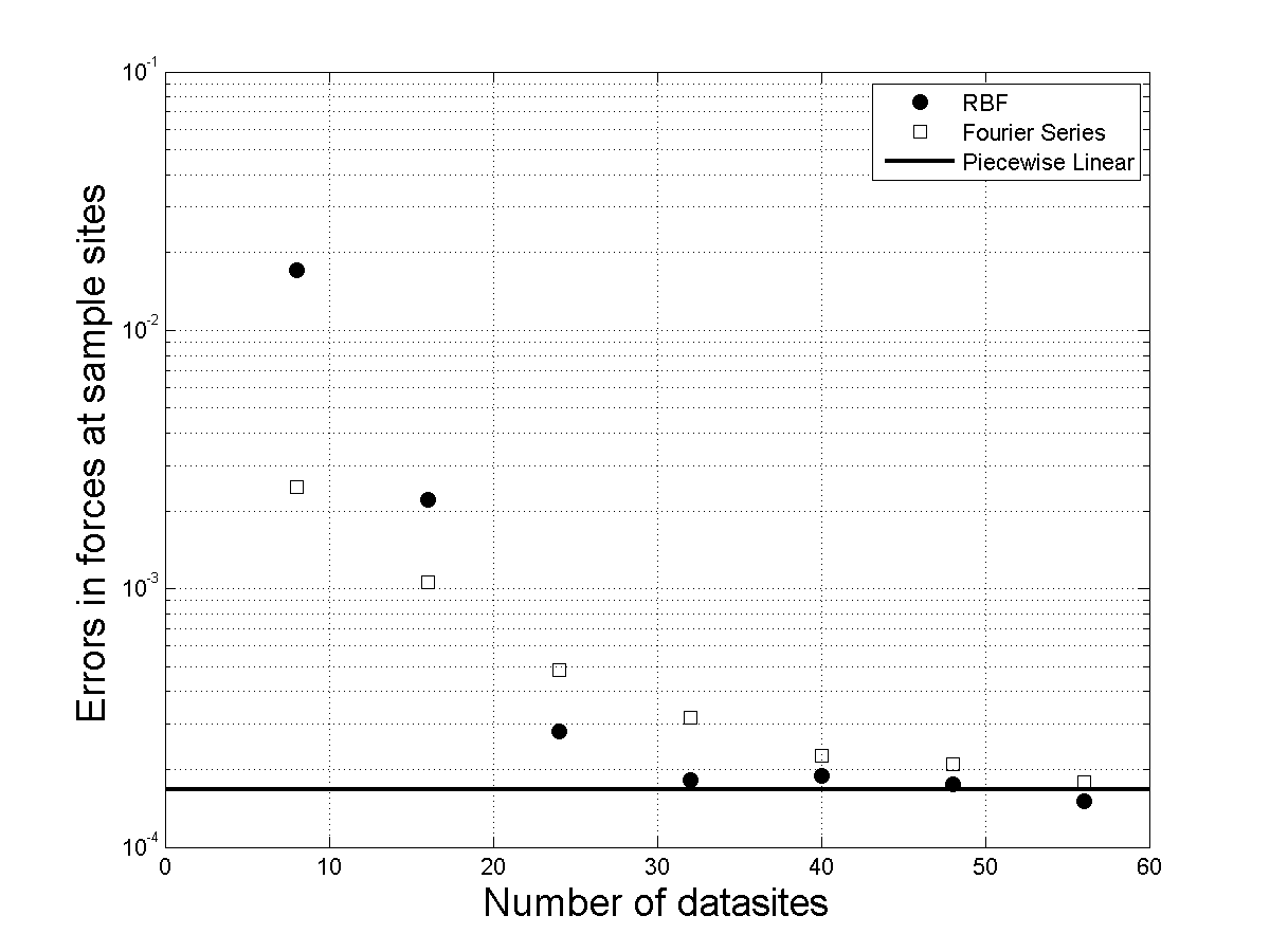
We lastly examine the errors in the force computation incurred by the two parametric models and the traditional piecewise linear model. Figure 9 shows the errors in forces evaluated at $100$ sample sites as a function of the number of data sites $N$. In all experiments, the force constant $K_{0}$ is set to $0.2$. The solid line in Figure 9 denotes the error for the piecewise linear model computed at $100$ IB points. For Object 1, we can see from the left plot of this figure that the errors for both parametric models are lower than the piecewise linear model starting at about $N=30$ data sites. Again, both the RBF and Fourier models give similar results for this object. For the non-smooth Object 2, it requires about $N=32$ data sites for the RBF model to match the errors of the piecewise linear model, while it takes approximately $N=56$ data sites for the Fourier model to give similar errors. We note that the errors for both the RBF and Fourier models do not fall as sharply for the non-smooth Object 2 as the number of datasites is increased. This is because Object 2 is generated from a function that has only two derivatives, and the force computation involves computing a second derivative. It therefore follows that these global methods would therefore not converge as they would in the case of the smooth Object 1.

Figure 9: Errors in the approximation of the forces evaluated at $M=100$ sample sites as a function of the number of data sites $N$ for Object 1 (left) and Object 2 (right). The black line denotes the errors for a piecewise linear model with $100$ IB points. Circles denote the errors for the RBF model and squares denote the errors for the Fourier model. For the RBF model, $\varepsilon=0.9$ for Object 1 and $\varepsilon=3.6$ for Object 2.

5.4 Comparison of the Computational Cost

We conclude the 2D results experiments with an examination of the computational cost associated with the three methods. We measure the computational cost as the elapsed wallclock time required to compute the interpolation coefficients, evaluate the interpolants, compute the normal vectors and compute the forces. Under the assumption that all objects will be evaluated at the same parametric sites at each timestep, for both parametric models we pre-compute the matrices for evaluating the interpolants, the derivatives, and the force operator once the interpolation coefficients have been determined (see Section 4.2 for details). We do not account for this setup time in our timing results.

Since for the piecewise linear model the number of evaluation sites is the same as the number of data sites, the total computational cost includes only the time required to compute the normal vectors and forces (see Section 4.1 for details).

All computations were performed in Matlab version 7.10.0499 (64-bit) on a Windows desktop with a Intel Core i7 Sandy Bridge 3.4 GHz processor and 4 GB of 1600 MHz RAM. Times were measured using the tic and toc functions in Matlab . All results presented are averages of a 100 trials and are in seconds.

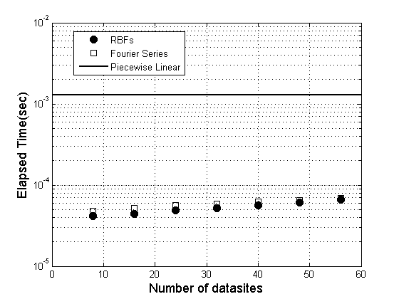
Figure 10 displays the elapsed time between the RBF, Fourier, and traditional piecewise linear models. The results for the RBF and Fourier models are displayed as a function of the number of data sites $N$ for a fixed number of $M=100$ sample sites. The results for the piecewise linear model are for a fixed number of $100$ IB points. We can see from the figure that the parametric models require significantly less time than the piecewise linear model. For $N=56$ data sites, the parametric models are over one order of magnitude faster.

Figure 10: Elapsed wallclock time (in seconds) for one object to perform interpolation, evaluation, the computation of normal vectors, and the computation of forces at $M=100$ sample sites as a function of the number of data sites $N$. The piecewise linear computations were done with $100$ IB points for comparison.

We note that all the evaluation and derivative computations for the parametric models can be formulated in terms of matrices in order to avoid the need to first solve for the coefficients every time step of the IB simulation. Thus, the results we present are not optimal in terms of computational time. If, however, during the IB simulation the sample sites change, then the step of going first through the coefficients as we have done will be necessary.

6 3D Platelet Modeling Results

Following a similar approach to the last section, we present here the results from a comparative study between using the traditional piecewise linear approach as used within the IB method and our two alternative parametric approaches in 3D: RBF and Fourier (spherical harmonics) interpolation. We examine the reconstruction capabilities of the models and the accuracy in computing normal vectors and forces. As in the 2D tests, we distinguish between data sites and sample sites. In all experiments unless otherwise specified, $M=1024$ sample sites are used as this represents the typical number of IB points that would be used per platelet object in a traditional 3D IB computation (and hence a reasonable standard against which to compare our new methods for the purposes of determining the feasibility of replacement). All errors are computed by taking the maximum of the two-norm difference between the approximations and the true values.

6.1 Test Cases

We again consider 2 prototypical test objects and define them based on perturbations of idealized shapes (an ellipsoid and a sphere). Let $\textbf{x}_{ideal}$ be a function representing the idealized, unperturbed shapes as given by the following equation:

$$\boldsymbol{x}_{ideal}=(x_{c}+a\cos\lambda\cos\theta,y_{c}+b\sin\lambda\cos\theta,z_{c}+c\sin\theta),$$ (46)

where $-\pi\leq\lambda\geq\pi$ and $-\frac{\pi}{2}\leq\theta\leq\frac{\pi}{2}$. Here $(x_{c},y_{c},z_{c})$ denotes the object center, $a$ and $b$ are the equatorial radii, and $c$ is the polar radius. The two objects used for our comparison are defined as follows:

$$\text{\text@underline{Object 1}: }\quad\boldsymbol{x}_{3d\,obj1} = \left[1.0+A\exp\left(\frac{r_{c}^{2}}{\sigma_{1}}\right)\right]\,\boldsymbol{x}_{ideal},$$ (47)

$$\text{\text@underline{Object 2}: }\quad\boldsymbol{x}_{3d\,obj2} = \left[1.0+B\exp\left(\frac{r_{c}^{2.5}}{\sigma_{2}}\right)\right]\,\boldsymbol{x}_{ideal}.$$ (48)

where $r_{c}=1-\cos\theta\cos\theta_{c}\cos(\lambda-\lambda_{c})-\sin\theta\sin\theta_{c}$. For Object 1, we use the following parameters: $x_{c}=y_{c}=z_{c}=0.9$, $a=0.1$, $b=0.2$, $c=0.09$, $A=0.09$ and $\sigma_{1}=0.2$. For Object 2, we use the following parameters: $x_{c}=y_{c}=0.1$, $z_{c}=0.2$, $a=b=c=0.1$, $B=0.04$ and $\sigma_{2}=\frac{16}{25}$. For both objects $\lambda_{c}=0$ and $\theta_{c}=\frac{\pi}{2}$.

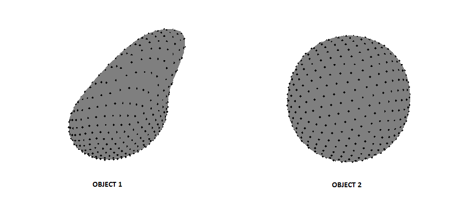
Figure 11 displays the two test objects (47) and (48). Object 1 is a smooth (in terms of regularity) yet highly perturbed ellipsoid, while the Object 2 is a non-smooth perturbation of a sphere. It can be shown that the parameterization (48) has only three continuous derivatives.

Figure 11: The test objects (47) and (48) for the 3D study.

6.2 Comparison of Reconstructing the Objects

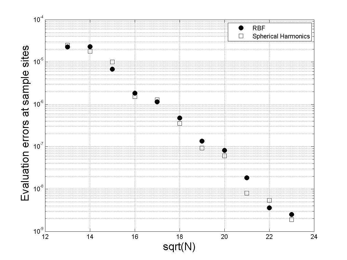
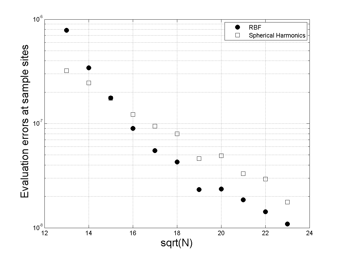
As in the 2D results, we first examine the errors in reconstructing the objects using the two parametric models. Figure 12 displays the errors in reconstructing the objects as a function of the square root of the number of data sites $N$. We use $\sqrt{N}$ since these are 2D objects and thus the reciprocal of this value gives a good measure of the spacing between data sites. These errors give a indication of the modeling capability of the RBF and Fourier methods. The results are similar to what we observed in 2D. For the smooth Object 1 (left plot in Figure 12), the RBF and Fourier models are converging at a spectral rate, but at a much slower rate for non-smooth Object 2. The RBF and Fourier models are giving similar errors for Object 1, with a few values of $N$ where the spherical harmonic method is clearly better. For Object 2, the RBF model consistently gives better results than the spherical harmonic model as $N$ increases. No direct comparison with the piecewise linear model is given as the piecewise linear IB method always samples at the interpolating points.

Figure 12: Error in the reconstruction of the shape of the objects (left is Object 1 and right is Object 2) evaluated at $M=1024$ sample sites as a function of the square root of the number of data sites $N$. Circles denote the errors in the RBF model and squares denote the errors for the Fourier model. For the RBF model, the shape parameter for Object 1 was set to $\varepsilon=0.9$ and for Object 2 was set to $\varepsilon=1.5$. Data sites for the RBF model are the ME points, while the data sites for the Fourier model are the MD points.

6.2.1 Shape Parameter Study

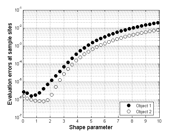
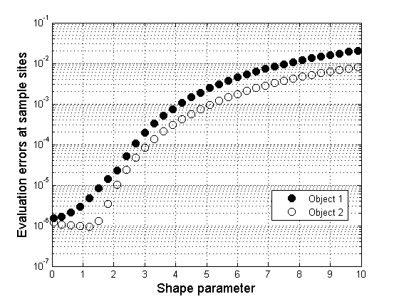
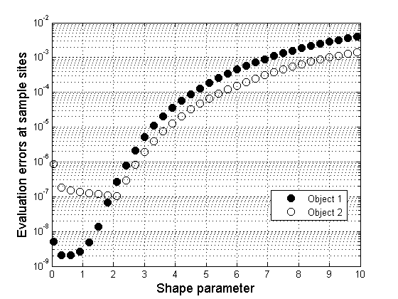
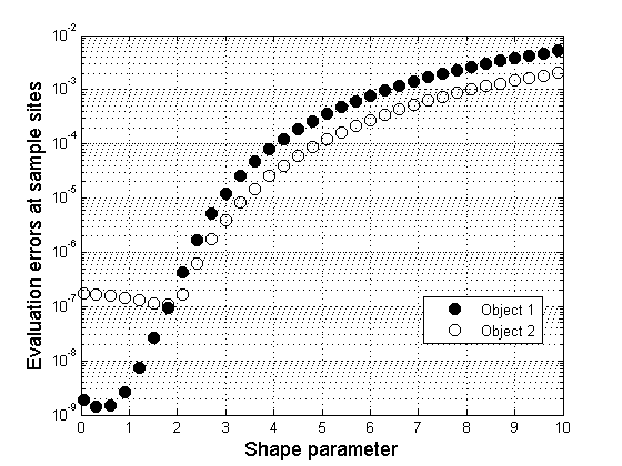
Figures 13 and 14 display the reconstruction errors of the RBF model for the two objects as a function of the shape parameter using $N=256$ data sites and $N=529$ data sites, respectively. The left plot of each of these figures contains the results for the ME points, while the right plot contains the results for the MD points. For $\varepsilon\lesssim 0.85$, it was necessary to use the RBF-QR algorithm [13] to compute the model in a numerically stable manner for the $N=529$ case. We see similar results to the 2D shape parameter study from Section 5.2.1. For the smooth Object 1 and the MD points the errors decrease rapidly as $\varepsilon$ decreases and reach a minimum near $\varepsilon=0$ (at $\varepsilon=0$ in the $N=256$ case), which correspond to a spherical harmonic interpolant on these nodes. For the ME points we see the error rise right as $\varepsilon$ gets to zero. For the non-smooth Object 2 and both types of nodes, we see that the error reaches a minimum at a larger value of $\varepsilon$ that is well within the numerically safe range of RBF-Direct. The errors then increase slightly as $\varepsilon$ decreases toward zero (with a jump up at $\varepsilon=0$ in the case of the ME points). From both Figures 13 and 14, we see that the errors in the RBF model are much better for the MD points when $\varepsilon$ is near zero, but as $\varepsilon$ increases away from zero the errors are better for the ME points.

We make similar comments to those at the end of Section 5.2.1 in regards to selection of the shape parameter for the 3D case, and thus refer the reader there.

Figure 13: Error in the shape at $1024$ sample sites as a function of the shape parameter for $256$ data sites on Object 1 (solid circles) and Object 2 (open circles) using minimal energy points (left) and maximal determinant points (right) for the data sites.

Figure 14: Error in the shape at $1024$ sample sites as a function of the shape parameter for $529$ data sites on Object 1 (solid circles) and Object 2 (open circles) using minimal energy points (left) and maximal determinant points (right) for the data sites.

6.3 Comparison of Normal Vectors and Forces

We next focus on the errors in the parametric models in the approximation of the normal vectors to the objects and the forces. In the case of computing the normal vectors, we compare the results to the traditional piecewise linear models based on triangulations of the surface. As discussed in Section 4.1, a comparison against the traditional piecewise linear 3D force model is not appropriate since this model is described purely algorithmically, and hence the underlying material constitutive model is not known and cannot be computed exactly even though the shape is known analytically.

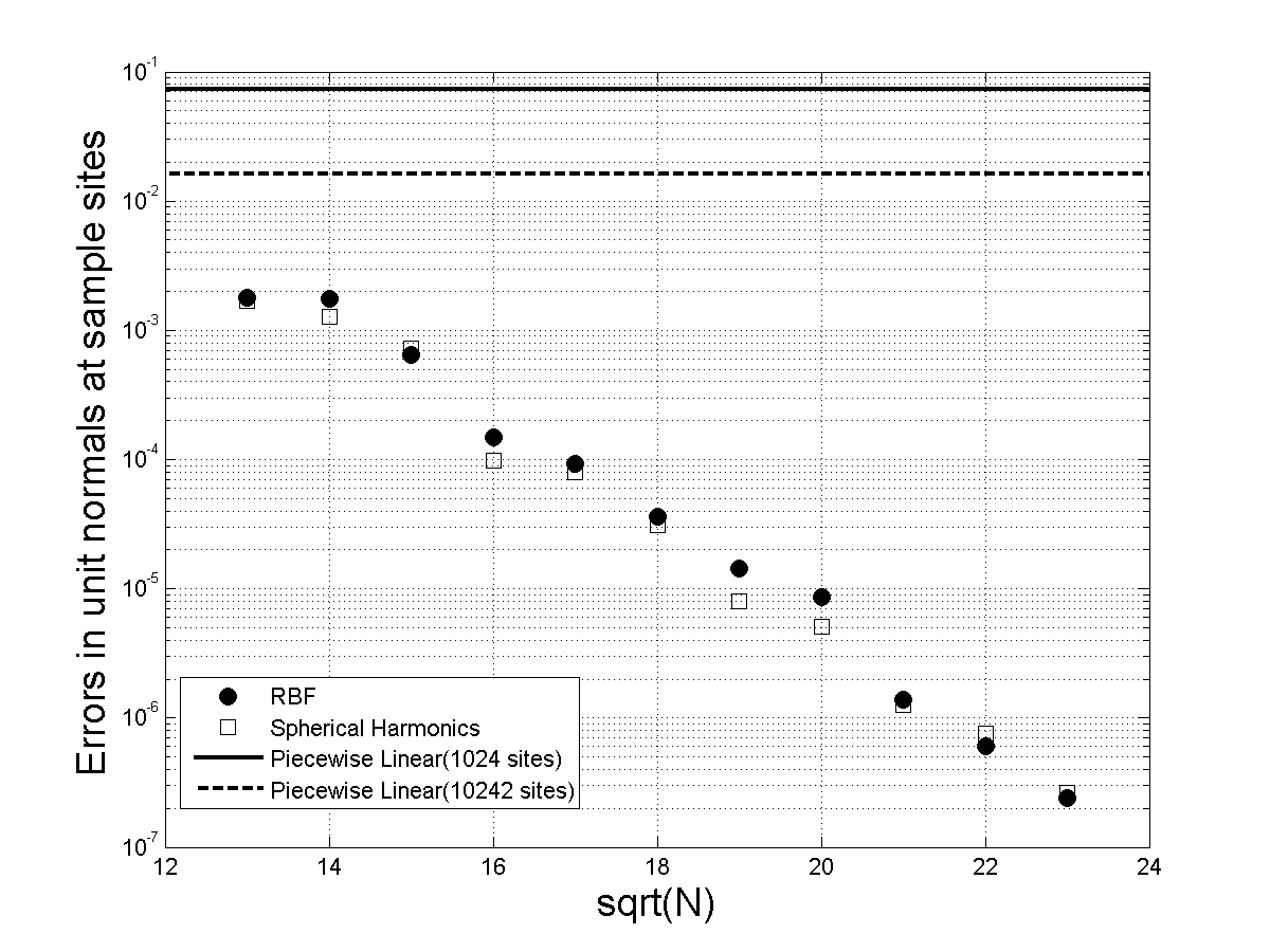
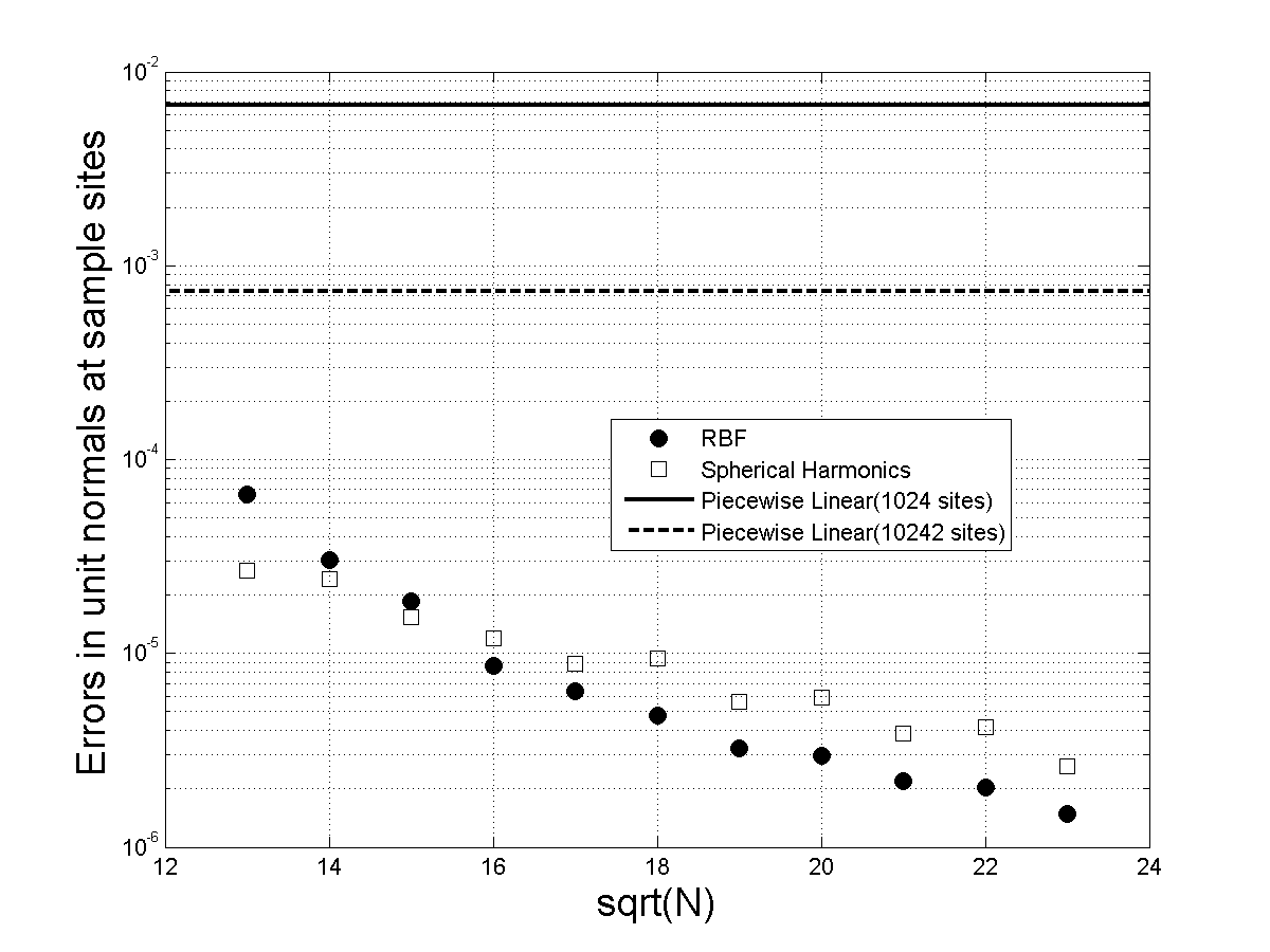
Figure 15 displays the errors in the normal vectors at $M=1024$ sample sites as a function of the square root of the number of data sites $N$. The solid and dashed lines in both plots from this figure denote the errors in the normal vectors at $1024$ and $10242$ IB points. We see that increasing the number of IB points, decreases the errors in the normal vectors. However, unlike the 2D case, both parametric models always give better results in the normal vector computations even for the high value of $10242$ IB points. Additionally, the errors in these computations for Object 1 are similar for the RBF and Fourier models. For Object 2, the RBF model gives consistently better results for increasing data sites $N$.

Figure 15: Errors in the approximations of the normal vectors to the 3D objects at $M=1024$ sample sites as a function of the square root of the number of data sites $N$. The left plot is for Object 1, while the right one is for Object 2. The solid line denotes the error for the method used in the piecewise linear model with $1024$ IB points and the dashed line corresponds to the error with $10242$ IB points. Circles denote the errors for the RBF model and squares denote the Fourier model. For the RBF model, $\varepsilon=0.9$ for Object 1 and $\varepsilon=1.5$. Data sites for the RBF model are the ME points, while the data sites for the Fourier model are the MD points.

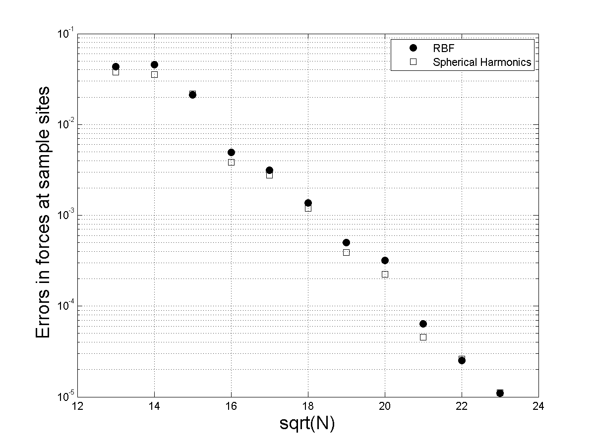
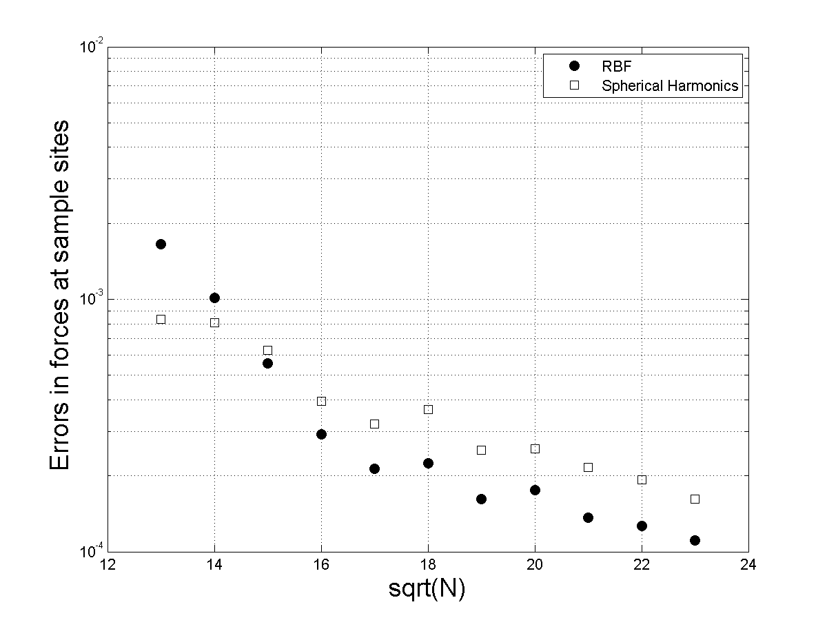
We lastly focus on the errors in the computation of the forces that occur in both parametric models. Figure 16 displays the errors in forces evaluated at $1024$ sample sites as a function of the square root of the number of data sites $N$. In all experiments, both the coefficient of surface tension $\gamma$ and the spring constant $K_{0}$ are set to 0.2. We see that the results between smooth and non-smooth objects are consistent with those from the shape reconstruction and normal vector approximations.

Figure 16: Errors in the approximations of the forces evaluated at $M=1024$ sample sites as a function of the square root of the number of data sites $N$ for Object 1 (left) and Object 2 (right). Circles denote the errors for the RBF model and squares denote the Fourier model. For the RBF model, $\varepsilon=0.9$ for Object 1 and $\varepsilon=1.5$. Data sites for the RBF model are the ME points, while the data sites for the Fourier model are the MD points.

6.4 Comparison of the Computational Cost

We conclude the 3D results experiments by examining the computational cost associated with the three methods. As in the 2D experiments, we measure the computational cost as the elapsed wallclock time required to compute the interpolation coefficients, evaluate the interpolants, compute the normal vectors and compute the forces. We pre-compute and store the $LU$ decomposition of the spherical harmonic interpolation matrix (11) and the Cholesky decomposition $LL^{T}$ of the RBF interpolation matrix (15). We also pre-compute matrices for evaluating the interpolants, the derivatives, and the force operator once the interpolation coefficients have been determined (see Section 4.2 for details). We do not account for these pre-computations in our timing results. As in 2D, all computations were performed in Matlab using the machine described in Section 5.4.

Since for the piecewise linear model the number of evaluation sites is the same as the number of data sites, the total computational cost includes only the time required to compute the normal vectors and forces (see Section 4.1 for details), we do not include the time to compute the triangulation of the surface.

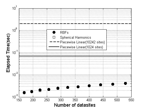
Figure 17 displays the elapsed time between the RBF, Fourier, and traditional piecewise linear models. The results for the RBF and Fourier models are displayed as a function of the number of data sites $N$ for a fixed number of $M=1024$ sample sites. Two results are presented for the piecewise linear model: one with $1024$ IB points (solid) line and one with $10242$ IB points (dashed line). We can see from the figure that the parametric models require significantly less time than the piecewise linear model, especially for the $10242$ case. For $N=529$ data sites, the parametric models are over one order of magnitude faster than the piecewise linear model with $1024$ IB points and nearly 3 orders of magnitude better with $10242$ IB points.

Figure 17: Elapsed wallclock time (in seconds) for one object to perform interpolation, evaluation, the computation of normal vectors, and the computation of forces at $M=1024$ sample sites as a function of the number of data sites $N$. The piecewise linear computations were done with $1024$ IB points (solid line) and $10242$ IB points (dashed line) for comparison.

7 Summary

The IB method is a common numerical methodology for applications involving fluid structure interactions. Our particular interest in this method is in simulating platelet aggregation during blood clotting. In this application, the platelets are modeled as immersed elastic structures whose shape changes dynamically in response to blood flow and chemistry. One of the fundamental ingredients of this application of the IB method (and many others involving immersed structures) is how to model the platelets geometrically, so that internal structural forces can be computed at specified locations on the platelet surface. The current strategy is to use piecewise linear models for representing the platelets. In this paper we have presented two alternative geometric models for platelets: RBFs and Fourier-based methods. Both of these models are based on a parametric representation of the surface using polar coordinates in 2D and spherical coordinates in 3D. This choice of parameterization is motivated by the observed shape of platelets both during their inactive and active states. We have described how these new models can be used for constructing and maintaining the platelet’s representation, computing the normal vectors to the platelet surface, and computing the internal structural forces. We have presented numerical comparisons between the traditional piecewise linear models and the new RBF and Fourier-based models in both 2D and 3D. Our findings indicate that both the RBF and Fourier methods provide viable alternatives to the traditional approach in terms of geometric modeling accuracy, force accuracy, and computational efficiency.

Although both the RBF and Fourier-based methods provided comparable results in terms of error characteristics and computational efficiency, we would advocate the use of the RBF-based models for the following reasons:

• they are easier to implement;

• they have accuracy similar to that of Fourier methods for smoothly-perturbed objects with similar computational costs;

• they are more accurate than Fourier methods for roughly perturbed objects with similar computational costs;

• they are more flexible than Fourier methods in terms of changing the underlying parameterizations of the objects (e.g. changing to an elliptical parameterization rather than polar) [14].

One issue with the RBF models is how to choose an appropriate shape parameter. We will study this issue as part of our next step in applying the RBF-based models in an IB simulation. This step will involve implementing the RBF-based models in a full IB simulation of platelet aggregation. The simulation will require projection of the forces from the sample points to the Eulerian mesh, computation of the Navier-Stokes system with forcing based upon the platelets, and then movement of the platelets via updating of the RBF data points. We will study how the shape parameter affects the simulations and compare the results of these simulations to those based on the traditional piecewise linear models for platelets.

Acknowledgments: We would like to acknowledge useful discussions concerning this work within the CLOT group at the University of Utah and with Prof. Robert Guy (UC-Davis). Support for this work came in part from NIGMS grant R01-GM090203 (VS, ALF, RMK), from NSF grant DMS-0540779 (ALF, GBW), and from NSF grant DMS-0934581 (GBW).

References

- [1] G. Agresar, J. J. Linderman, G. Tryggvason, K. G. Powell, An adaptive, cartesian, front-tracking method for the motion, deformation and adhesion of circulating cells, Journal of Computational Physics 143 (1998) 346–380.
- [2] R. P. Beyer, A computational model of the cochlea using the immersed boundary method, Journal of Computational Physics 98 (1992) 145–162.
- [3] R. Dillon, L. Fauci, A. Fogelson, D. Gaver, Modeling biofilm processes using the Immersed Boundary method, Journal of Computational Physics 129 (1996) 85–108.
- [4] G. E. Fasshauer, Meshless Approximation Methods with MATLAB, Interdisciplinary Mathematical Sciences - Vol. 6, World Scientific Publishers, Singapore, 2007.
- [5] G. E. Fasshauer, L. L. Schumaker, Scattered data fitting on the sphere, in: M. Daehlen, T. Lyche, L. L. Schumaker (eds.), Mathematical Methods for Curves and Surface, Vol.2 of the Proceedings of the 4th Int. Conf. on Mathematical Methods for Curves and Surfaces, Lillehammer, Norway, Vanderbilt University Press, Nashville Tennessee, 1998.
- [6] L. J. Fauci, A. L. Fogelson, Truncated newton methods and the modeling of complex immersed elastic structures, Communications on Pure and Applied Mathematics 66 (1993) 787–818.
- [7] L. J. Fauci, C. S. Peskin, A computational model of aquatic animal locomotion, Journal of Computational Physics 77 (1988) 85–108.
- [8] N. Flyer, G. B. Wright, Transport schemes on a sphere using radial basis functions, J. Comp. Phys. 226 (2007) 1059–1084.
- [9] N. Flyer, G. B. Wright, A radial basis function method for the shallow water equations on a sphere, Proc. Roy. Soc. A 465 (2009) 1949–1976.
- [10] A. L. Fogelson, A mathematical model and numerical method for studying platelet adhesion and aggregation during blood clotting, Journal of Computational Physics 1 (1984) 111–134.
- [11] A. L. Fogelson, R. D. Guy, Immersed-boundary-type models of intravascular platelet aggregation, Computer Methods in Applied Mechanics and Engineering 197 (2008) 2087 – 2104.
- [12] B. Fornberg, A Practical Guide to Pseudospectral Methods, Cambridge University Press, Cambridge, 1996.
- [13] B. Fornberg, C. Piret, A stable algorithm for flat radial basis functions on a sphere, SIAM J. Sci. Comp. 30 (2007) 60–80.
-
[14]
E. Fuselier, G. Wright, Scattered data interpolation on embedded submanifolds
with restricted positive definite kernels: Sobolev error estimates, SIAM
Journal on Numerical Analysis 50 (3) (2012) 1753–1776.
URL http://epubs.siam.org/doi/abs/10.1137/110821846 - [15] Q. T. L. Gia, Approximation of parabolic pdes on spheres using spherical basis functions, Adv. Comput. Math. 22 (2005) 377–397.
- [16] G. H. Golub, C. F. van Loan, Matrix Computations, 3rd ed., Johns Hopkins University Press, Baltimore, 1996.
- [17] A. Gray, Modern Differential Geometry of Curves and Surfaces with Mathematica, CRC Press, Boca Raton, FL, 1997.
- [18] D. P. Hardin, E. B. Saff, Discretizing manifolds via minimum energy points, Notices Amer. Math. Soc. 51 (2004) 1186–1194.
[19]
S. Hubbert, T. M. Morton, -error estimates for radial basis function
interpolation on the sphere, J. Approx. Theory 129 (2004) 58–77.
URL http://portal.acm.org/citation.cfm?id=1022246.1022249 - [20] S. Hubbert, S. Müller, Interpolation with circular basis functions, Numerical Algorithms 42 (2006) 75–90.
- [21] K. Jetter, J. Stöckler, J. D. Ward, Error estimates for scattered data interpolation on spheres, Math. Comput. 68 (226) (1999) 733–747.
- [22] L. A. Miller, C. S. Peskin, When vortices stick: an aerodynamic transition in tiny insect flight, The Journal of Experimental Biology 207 (2004) 3073–3088.
- [23] L. A. Miller, C. S. Peskin, A computational fluid dynamics of ’clap and fling’ in the smallest insects, The Journal of Experimental Biology 208 (2005) 195–212.
- [24] F. J. Narcowich, X. Sun, J. D. Ward, H. Wendland, Direct and inverse Sobolev error estimates for scattered data interpolation via spherical basis functions, Found. Comput. Math. 7 (3) (2007) 369–390.
- [25] E. P. Newren, A. L. Fogelson, R. D. Guy, R. M. Kirby, Unconditionally stable discretizations of the immersed boundary equations, Journal of Computational Physics 222 (2007) 702–719.
- [26] C. S. Peskin, Numerical analysis of blood flow in the heart, Journal of Computational Physics 25 (1977) 220–252.
- [27] C. S. Peskin, The immersed boundary method, Acta Numerica 11 (2002) 479–517.
- [28] C. S. Peskin, D. M. McQueen, Modeling prosthetic heart valves for numerical analysis of blood flow in the heart, Journal of Computational Physics 37 (1980) 113–132.
- [29] C. S. Peskin, D. M. McQueen, A three-dimensional computational method for blood flow in the heart: I. immersed elastic fibers in a viscous incompressible fluid, Journal of Computational Physics 81 (1989) 372–405.
- [30] S. Rippa, An algorithm for selecting a good value for the parameter c in radial basis function interpolation, Adv. Comput. Math. 11 (1999) 193–210.
- [31] L. Shen, H. Farid, M. A. McPeek, Modeling three-dimensional morphological structures using spherical harmonics, Evolution 4 (63) (2009) 1003–1016.
- [32] G. Thürmer, C. A. Wüthrich, Computing vertex normals from polygonal facets, journal of graphics, gpu, and game tools 3 (1) (1998) 43–46.
- [33] L. N. Trefethen, Spectral Methods in MATLAB, Society for Industrial and Applied Mathematics, Philadelphia, PA, USA, 2000.
- [34] H. Wendland, Scattered data approximation, vol. 17 of Cambridge Monographs on Applied and Computational Mathematics, Cambridge University Press, Cambridge, 2005.
- [35] R. S. Womersley, I. H. Sloan, How good can polynomial interpolation on the sphere be?, Adv. Comput. Math. 23 (2001) 195–226.
- [36] R. S. Womersley, I. H. Sloan, Interpolation and cubature on the sphere, Website, http://web.maths.unsw.edu.au/ rsw/Sphere/ (2007).
- [37] J. Yang, An embedded-boundary formulation for large-eddy simulation of turbulent flows interacting with moving boundaries, Ph.D. thesis, University of Maryland, College Park, College Park, Maryland (2005).
[38]
L. Yao, A. L. Fogelson, Simulations of chemical transport and reaction in a
suspension of cells i: an augmented forcing point method for the stationary
case, International Journal for Numerical Methods in Fluids 69 (11) (2012)
1736–1752.
URL http://dx.doi.org/10.1002/fld.2661