The geometry of percolation fronts in two-dimensional lattices with spatially varying densities

Abstract

Percolation theory is usually applied to lattices with a uniform probability $p$ that a site is occupied or that a bond is closed. The more general case, where $p$ is a function of the position $x$, has received less attention. Previous studies with long-range spatial variations in $p(x)$ have only investigated cases where $p$ has a finite, non-zero gradient at the critical point $p_{c}$. Here we extend the theory to two-dimensional cases in which the gradient can change from zero to infinity. We present scaling laws for the width and length of the hull (i.e. the boundary of the spanning cluster). We show that the scaling exponents for the width and the length depend on the shape of $p(x)$, but they always have a constant ratio $4/3$ so that the hull’s fractal dimension $D=7/4$ is invariant. On this basis, we derive and verify numerically an asymptotic expression for the probability $h(x)$ that a site at a given distance $x$ from $p_{c}$ is on the hull.

1 Introduction

Percolation theory is a powerful tool in describing systems of randomly located objects that are placed on the sites or bonds of a network [1]. The sites or bonds are independently occupied with a probability $p$ or remain vacant with probability $1-p$. The task of percolation theory is to identify the properties of the clusters formed by the connected components. In most theoretical studies, $p$ is assumed to be equal everywhere (i.e. the system is assumed to be uniform). However, in many real-world applications, it is more natural to allow some variation in $p$ among the sites or bonds. In spatial systems, $p$ often depends on the position. For example, if occupied sites represent particles that diffuse from the right-hand edge of a two-dimensional lattice and are absorbed on the left-hand edge, then the concentration of particles exhibits a gradient [2] and the system looks qualitatively like the lattice in figure 1. Gradients also frequently arise in the spatial distribution of biological populations because the environmental conditions may change gradually in space (e.g. from lower to higher elevation along a hillside). If occupied sites represent the presence of a species, the population can exhibit a spatial transition from isolated individuals to a large connected component [3, 4].

Figure 1: Site percolation on a triangular lattice where occupied sites (grey hexagons) are more abundant towards increasing $x$-coordinates. The hull (black curve) marks the boundary between the vacant spanning cluster on the left and the occupied spanning cluster on the right. The hull width $w$, defined in (1), is the standard deviation in the hull’s $x$-coordinates.

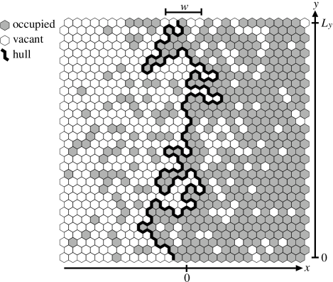
Given such a transition in connectivity, the focus of gradient percolation is on the hull [5], defined as the interface between adjacent occupied and vacant clusters that both fully span the lattice’s $y$-direction (black curve in figure 1). The hull has been used in practice, for example, in studies of the surface structure of polymers [7], of the treeline dividing woodland from grassland [3, 4], of the boundary of urban settlements [8] and as an example of a non-trapping self-avoiding random walk whose properties have been investigated theoretically [9, 10] and with computer simulations [11, 12]. Apart from its many applications, gradient percolation is also an active field of theoretical investigation. It allows highly accurate measurements of the smallest occupancy probability $p_{c}$ for which an infinite spanning cluster of occupied sites exists. The value of $p_{c}$ is equal for gradient and non-gradient (i.e. uniform) lattices. Introducing a gradient has the advantage that $p$ does not need to be carefully fine-tuned to achieve excellent numerical results [13, 14]. Furthermore, the geometry of the hull is particularly intriguing. Suppose the hull connects the sequence of coordinates $(x_{1},y_{1}=0),\ldots,(x_{l},y_{l}=L_{y})$ delineating the boundary of the spanning cluster, where $L_{y}$ is the system size in the $y$-direction. If $p$ can be approximated near $p_{c}$ by a linear function $p(x)=ax+p_{c}$, then the hull width $w$, defined as the standard deviation of the hull’s $x$-coordinates,

$$w=\sqrt{\frac{\sum_{i}x_{i}^{2}}{l}-\left(\frac{\sum_{i}x_{i}}{l}\right)^{2}},$$ (1)

is known to scale as $a^{-4/7}$ in the limit $a\to 0$. The hull length $l$ is proportional to $L_{y}a^{-3/7}$ and, on length scales below $w$, the hull’s fractal dimension is $D=7/4$ [2]. These non-trivial scaling laws – recently proved rigorously by Nolin [15, 16] – have sparked a lot of interest (see [17] for a survey of the literature) and some researchers have generalized the results to gradients in more complicated lattice models [18, 19, 20, 21, 22, 23]. So far, all studies have assumed that $p(x)$ can be treated, at least locally, as a linear function (figure 2(a)). However, this is frequently not the case in reality. As $a\to 0$, higher order terms in the Taylor expansion of $p$ may become dominant so that $w$ and $l$ do not diverge, although this is predicted when interpreting $w\propto a^{-4/7}$ and $l\propto L_{y}a^{-3/7}$ literally. Local linearization is not possible either if the gradient does not exist at all, for instance if $p$ jumps discontinuously from one value to another.

Figure 2: The studied occupancy probabilities $p(x)$. (a): Linear function. This has been, at least as a local approximation, the assumption in all previous studies of gradient percolation. (b): Discontinuous function ($b=0$ in (2)). (c) and (d): Continuous function with infinite or zero slope at $x=0$ ($0<b<1$ or $b>1$, respectively).

Here we examine representative cases in which no linear approximation for $p(x)$ exists at $p_{c}$. We investigate the class of functions

$$p(x)=\cases{\max(0,\,p_{c}-a(-x)^{b})&if $x<0$,\cr\min(1,\,p_{c}+ax^{b})&if $x\geq 0$\cr}$$ (2)

for $b\geq 0$ and $a>0$. If $b=0$, $p(x)$ makes a discontinuous jump over the percolation threshold $p_{c}$ (figure 2(b)). For $0<b<1$, $p(x)$ is continuous, but the gradient at $p_{c}$ is infinite (figure 2(c)). If $b>1$, the gradient is zero (figure 2(d)), so that $|p(x)-p_{c}|$ approaches zero faster than any linear function at $x=0$. We have chosen the coefficient $a$ in (2) to be equal on the positive and negative $x$-axis. This is a convenient choice because, as we show below, the probability to find the hull at a coordinate $x$ is in this case symmetric about $x=0$. The results described below can be easily generalized to cases where the coefficients differ in the positive and negative direction. We present numerical simulations for site percolation on triangular lattices, where $p_{c}=1/2$, and apply periodic boundary conditions in the $y$-direction ($L_{y}\geq 4096$). For a comparison, we also performed simulations for site and bond percolation on square lattices. We found the same scaling exponents, indicating that they are independent of the lattice type and presumably also valid in continuum models [24].

2 Hull width, length and fractal dimension

Figure 3: Illustration of the relation between hull width $w$ and correlation length $\xi$ near $x=0$, where the hull meanders between islands of vacant and occupied sites. The linear size of these obstacles is of the order of $\xi$. Therefore, the hull width $w$, which measures the fluctuations of the hull around $x=0$, is also approximately $\xi$.

Figure 4: (a) The hull width $w$ versus $a$ for different values of $b$ in (2) from computer simulations (shown as circles, squares, and diamonds). The lines indicate the expected power law $w\propto a^{-B}$ with $B=\nu/(\nu b+1)$. The number next to each line states the value of $B$. Error bars are smaller than the symbol sizes. (b) The normalized hull length $l/L_{y}$ scales $\propto a^{-C}$ with $C=1/(\nu b+1)$ as displayed by the lines. (c) The fractal dimension $D$ of the hull is determined with the equipaced polygon method [25] described in the appendix. In this method, we compute the mean Euclidean distance $\bar{d}(k)$ between hull coordinates that are $k$ steps apart. A numerical estimate of $D$ can be obtained by fitting $\bar{d}(k)\propto k^{1/D}$. We observe that $D=7/4$ is independent of $b$. Inset: $D=1.75$, numerically calculated as the derivative $\rmd(\log k)/\rmd(\log\bar{d})$, is within the error bars for almost three orders of magnitude of $k$.

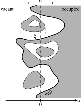
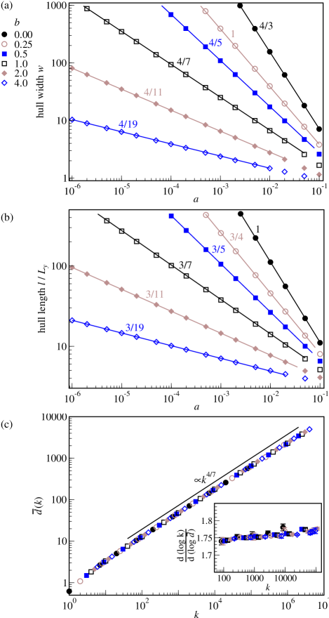
Let us first consider the hull width $w$ in the discontinuous case ($b=0$ in (2)). Because $a>0$, the hull must navigate around those occupied clusters to the left that are not part of the occupied spanning cluster (figure 3). Similarly, on the right-hand side, excursions of the hull must steer clear of smaller vacant islands that have not merged with the vacant spanning cluster. The typical linear size of these smaller clusters is given by the correlation length $\xi$ which scales in uniform systems $\propto|p-p_{c}|^{-\nu}$ if $p\approx p_{c}$. Because the critical exponent $\nu$ is equal to $4/3$ in two dimensions [1, 26] and because the hull width scales in proportion to the cluster sizes, we expect $w\propto a^{-4/3}$. Our numerical simulations confirm this intuition (black filled circles in figure 4a).

If $b>0$, the situation is more complicated because $p(x)$, and hence also $\xi(p(x))$, change gradually as a function of $x$. For $b=1$, Sapoval et al. [2] have pointed out that we can still derive the correct scaling behaviour by assuming that $w$ is proportional to the correlation length at $w$. The self-consistent relation $w\propto\xi(p(w))$, where the local correlation length satisfies $\xi(p(x))\propto|p(x)-p_{c}|^{-\nu}$ and $p(x)=p_{c}+ax$, yields the aforementioned $w\propto a^{-\nu/(\nu+1)}=a^{-4/7}$ (black open squares in figure 4a). Carrying out the calculation more generally for $p(x)$ given by (2) with arbitrary $b$ and assuming $a$ to be small, we obtain

$$w\propto a^{-\nu/(\nu b+1)}.$$ (3)

The same self-consistency requirement has been noticed and tested for the Ising quantum chain [28, 29], where the exponent $\nu$ however has a value different from the exponent in percolation. In figure 4(a), we compare data from numerical simulations with the prediction of equation (3) based on the two-dimensional percolation exponent $\nu=4/3$. The data show excellent agreement.

There is a similar scaling relation between the normalized hull length $l/L_{y}$ and $a$, where $l$ is the number of steps in the hull in a lattice of vertical dimension $L_{y}$. The scaling of $l/L_{y}$ cannot be derived as intuitively as the scaling of the hull width. However, previous numerical evidence in the case $b=1$ has supported the hypothesis $l/L_{y}\propto a^{-3/7}$ [2], now known to be correct [15]. For arbitrary $b$, our data (figure 4b) indicate the more general relation

$$l/L_{y}\propto a^{-1/(\nu b+1)},$$ (4)

which includes the scaling law for $b=1$ as a special case.

The scaling of $l$ and $w$ is related to the fractal dimension $D$ of the hull as follows. For a given value $a=a_{1}$ and system size $L_{y,1}$, let us denote the hull length by $l_{1}$ and the width by $w_{1}$. If we coarse-grain the hull by measuring it with rulers whose length is $A$ times longer than the lattice constant, we need $l_{2}\propto A^{-D}l_{1}$ rulers to cover the full length of the hull [30]. The width and the system size, however, are linear objects: it requires $w_{2}\propto A^{-1}w_{1}$ rulers to span across the hull’s $x$- and $L_{y,2}\propto A^{-1}L_{y,1}$ rulers to cover its $y$-extent. Thus, measured in units that are increased by a factor $A$, the hull length, width and system size all appear smaller by either a factor $A^{-D}$ or $A^{-1}$. Now suppose that the hull geometry scales as $w\propto a^{-B}$ and $l\propto L_{y}a^{-C}$. We obtain the same $w_{2}$ and $L_{y,2}$ as before if the lattice constant remains our fundamental length scale, but we first replace $a_{1}$ by $a_{2}\propto A^{1/B}a_{1}$ and then, from the original system of length $L_{y,1}$, we cut out a strip of size $A^{-1}L_{y,1}$. In this geometry $l_{2}\propto(A^{-1}L_{y,1})(A^{-C/B}a_{1}^{-C})\propto A^{-(1+C/B)}l_{1}$. Comparing this with our previous expression for $l_{2}$, we conclude that

$$D=1+\frac{C}{B}.$$ (5)

Inserting $B=\nu/(\nu b+1)$ and $C=1/(\nu b+1)$ from equations (3) and (4) we find $D=1+1/\nu=7/4$, independent of $b$. We also measured the fractal dimension directly using an independent numerical method (following [25, 12] and outlined in the appendix) and again find good agreement with $D=7/4$ (figure 4c). The fractal dimension of cluster hulls has recently received a lot of interest. In uniform percolation, where $p=p_{c}$ at all sites (i.e. $a=0$ in (2)), $D=7/4$ is now known to be exact, thanks to mathematical advances in stochastic Loewner evolution [26]. Recent work by Nolin and Werner [27] proves that the Hausdorff dimension remains $7/4$ if $p$ is near, but not exactly equal to $p_{c}$. In constant gradients ($b=1$ in (2)), $D=7/4$ was already conjectured in early studies [2] and related to the scaling of $w$ and $l$. Our results demonstrate that $D=7/4$ holds much more generally. Although $B=\nu/(\nu b+1)$ and $C=1/(\nu b+1)$ depend on $b$ and thus differ in the different scenarios depicted in figure 2, the ratio $B/C=\nu$ and hence the fractal dimension $D=1+1/\nu$ are invariant properties of the hull geometry.

3 Hull density profile

Figure 5: (a) Hull density $h$ as a function of position $x$ for $b=0$ in equation (2). Inset: data collapse for $\tilde{h}(\tilde{x})=a^{(1-\nu)(\nu b+1)}h(a^{-\nu/(\nu b+1)}\tilde{x})$. (b) Hull density for a piecewise continuous function $p(x)$ with multiple discontinuities. The local value of $p(x)$ is given by the grey numbers under the graph. In every interval of constant $p$, $h$ is approximately exponential, resulting in straight lines in this logarithmic plot. (c) Hull density for $b=4$.

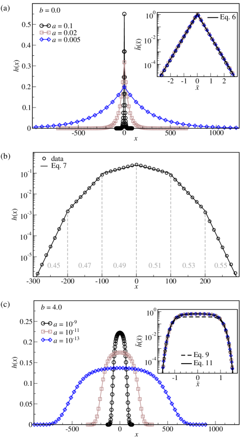
The hull width and length are simple measures of the hull geometry, but the distribution of the hull’s $x$-coordinates contains yet more information. For fixed $x$, we define the hull density $h(x)$ as the fraction of coordinates $(x,y)$ in the lattice that are on the hull. We focus first on the case $b=0$ where $p(x)=p_{c}\mp a$ provided that $a$ is sufficiently small. The $\mp$ sign is to be interpreted as a minus (plus) sign for negative (positive) $x$. Our simulations for $b=0$ show that $h(x)$ has a maximum at $x=0$ and falls off exponentially and symmetrically to both sides (figure 5a),

$$h(x)=E_{0}a^{\nu-1}\exp(-Fa^{\nu}|x|),$$ (6)

where $E_{0}$ and $F$ are positive constants. The exponential decay of $h(x)$ is reminiscent of the off-critical correlation function $g_{c}(\mathbf{r})\propto\exp(-|\mathbf{r}|/\xi)$ in uniform percolation, where $g_{c}(\mathbf{r})$ denotes the probability that $\mathbf{r}$ and the origin are part of the same finite cluster. The decay rate $(Fa^{\nu})^{-1}$ has the same scaling as the correlation length $\xi$, namely $\propto|p-p_{c}|^{-\nu}$ for both $p<p_{c}$ and $p>p_{c}$. However, there is one important difference between $(Fa^{\nu})^{-1}$ and the correlation length. In uniform percolation, $\xi$ has different amplitudes on the sub- and supercritical branch [31]. By contrast, we observe that $F$ is equal for $x<0$ and $x\geq 0$.

Equation (6) has several interesting consequences. First, $h(x)$ is a symmetric function (i.e. $h(x)=h(-x)$). We observed this symmetry in all investigated lattice types (triangular site percolation, square site and bond percolation). Second, (6) is consistent with the scaling relations (3) and (4) of the width and length for $b=0$. This can be proved by inserting (6) into $l=\int_{-\infty}^{\infty}h(x)dx$ and $w^{2}=\int_{-\infty}^{\infty}(x^{2}h(x)dx)/l$. Third, after appropriate rescaling of $h$, the function $\tilde{h}(\tilde{x})=a^{1-\nu}h(a^{-\nu}\tilde{x})$ is independent of $a$ (see the data collapse in the inset of figure 5(a)).

The case $b>0$, where $p(x)$ changes continuously, requires a little more effort than $b=0$, where $p(x)$ is constant except for one discontinuity. Our goal is to approximate $h(x)$ for $b>0$ by discretizing $p(x)$. To this end, let us consider the intermediate case where $p$ has more than one discontinuity: $p(x)=0$ for $x<x_{1}$, $p(x)=\pi_{1}$ for $x\in[x_{1},x_{2})$, $\ldots$, $p(x)=\pi_{n-1}$ for $x\in[x_{n-1},x_{n})$ and $p(x)=1$ for $x_{n}\leq x$ with $0<\pi_{1}<\ldots\pi_{n-1}<1$. Let us assume that the length $(x_{i}-x_{i-1})$ of each plateau is larger than the exponential decay length $(F|\pi_{i}-p_{c}|^{\nu})^{-1}$. In this case, $h$ consists of piecewise exponential functions $\propto\exp(\pm F|\pi_{i}-p_{c}|^{\nu}x)$ that are continuously joined together at the breakpoints $x_{1},\ldots,x_{n}$ (an example is shown in figure 5b). In terms of a differential equation, we can express this as

$$\frac{\rmd}{\rmd x}\log h(x)=\pm F|p(x)-p_{c}|^{\nu},$$ (7)

where $F$ is a constant. The plus sign holds for $p(x)<p_{c}$; otherwise the minus sign applies.

We now make two approximations to obtain an analytic expression for $h(x)$ if $p(x)$ changes continuously. First we assume that the rate of change in $p(x)$ is small compared to the characteristic decay length $(F|p(x)-p_{c}|^{\nu})^{-1}$ for all $x$. This allows us to insert (2) directly into (7). We obtain

$$\frac{\rmd}{\rmd x}\log h(x)=\pm Fa^{\nu}(\mp x)^{\nu b}$$ (8)

for $x$ in the interval $[-(p_{c}/a)^{1/b},((1-p_{c})/a)^{1/b}]$. We know from (3) that the hull width is a vanishing fraction of the width of this interval for $a\to 0^{+}$. Thus, our second approximation consists of extending (8) over the entire real line. The solution is

$$h(x)=E_{b}a^{(\nu-1)/(\nu b+1)}\exp\left(-\frac{F}{\nu b+1}a^{\nu}|x|^{\nu b+1}\right),$$ (9)

where we have factored out $a^{(\nu-1)/(\nu b+1)}$ from the integration constant so that, according to (4), the remaining factor $E_{b}$ does not depend on $a$.

4 Discussion

Straightforward integration proves that (9) is consistent with the scaling of the hull width in (3). Because (9) also satisfies the scaling of the length (4), it implies the correct fractal dimension $7/4$ according to (5). In addition to the scaling laws, (9) also provides an analytic expression for the functional form of the hull density profile: $h(x)$ is, in this approximation, proportional to a generalized normal distribution [32]. For $b=1/\nu$, we predict a Gaussian profile. Another special case is $b=0$, where we retrieve the Laplace distribution of (6). For $0\leq b<1/\nu$ the distribution is leptokurtic (i.e. it has a narrower peak and fatter tails than a Gaussian); for $b>1/\nu$ it is platykurtic (broader peak, thinner tails).

Figure 6: The transformation from $h$ to $f_{b}$ according to (10) shows that the hull density decays as $\exp(-Fa^{\nu}x^{\nu b+1}/(\nu b+1))$ with the same factor $F\approx 4.3$ for all $b$.

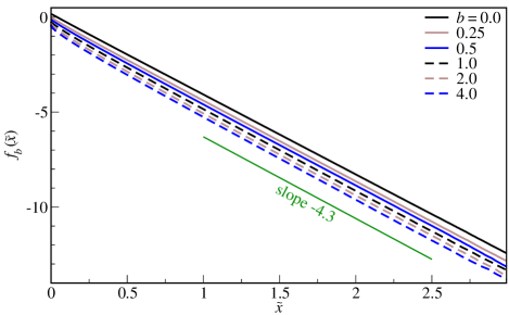
For any particular $b$ in (9), the rescaled hull density $\tilde{h}(\tilde{x})=a^{(1-\nu)/(\nu b+1)}h(a^{-\nu/(\nu b+1)}\tilde{x})$ is independent of $a$ (insets in figures 5(a) and 5(c)). Rescaling can even go further. Above we have assumed that the constant $F$ in (7) is independent of $b$ so that the functions

$$f_{b}(\tilde{x})=\log\{a^{(1-\nu)/(\nu b+1)}h[((\nu b+1)a^{-\nu}\tilde{x})^{1/(\nu b+1)}]\}$$ (10)

ought to be linear functions with the same slope $-F$ for all $b$. Figure 6 demonstrates that this is indeed true for $\tilde{x}\gtrsim 1$, which is valid if $x\gtrsim w$. From linear regression to $f_{b}$, we estimate $F=4.3\pm 0.1$.

For $b\ll 1$, a simple line in figure 6 fits the data very well for all $\tilde{x}>0$ and this is presumably exact for $b=0$. However, as $b$ becomes larger, there are visible departures from the asymptotic line for $\tilde{x}\ll 1$. In this regime, $p(x)$ varies significantly over length scales comparable to the correlation length, thus violating the assumption behind (8). If $b\gg 1$, we are effectively dealing with a system at the critical point confined to the strip $-(p_{c}/a)^{1/b}<x<((1-p_{c})/a)^{1/b}$. Some properties of critical cluster geometry in a strip are known exactly [33, 34, 35]. From the known results for the “one-pinch point density” in rectangular domains [36], it is plausible that $h(x)$ is analytic and has a Taylor expansion around $x=0$ with leading terms $h(x)=h(0)+h^{\prime\prime}(0)x^{2}/2+O(x^{4})$ and $h^{\prime\prime}(0)<0$. As a consequence, as $x\to 0$ we expect $\log(h)$ to be approximately quadratic (i.e. $\log(h(x))\approx G_{0}-H_{0}x^{2}$), in contrast to $\log(h(x))\approx G_{\infty}-H_{\infty}|x|^{\nu b+1}$ for $|x|\to\infty$ as predicted by (9).

Figure 7: If the hull density is locally approximated as a function proportional to $\exp(-H|x|^{J})$, the best fitting exponent $J$ increases as $\nu b+1$ in the tail (i.e. as $x\to\infty$), but is close to $2$ for $b>3/4$ in the core (i.e. as $x\to 0$).

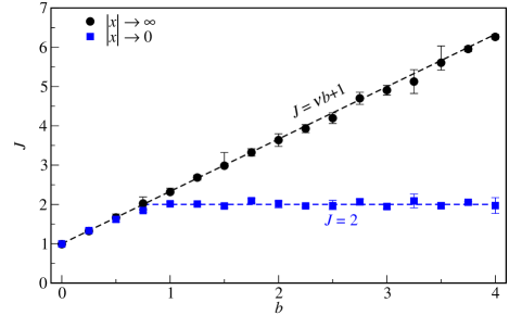
We test this hypothesis with nonlinear least-squares regressions of the general form $G-H|x|^{J}$ to fit either the core or the tail of $\log(h(x))$. The best fitting exponents for $|x|\to\infty$ are indeed consistent with $J=\nu b+1$ (figure 7) for all $b$. Performing the regression around $x=0$, on the other hand, we find a crossover from $J=\nu b+1$ to $J=2$ at $b\approx 1/\nu=3/4$. This suggests that for $b<1/\nu$, (9) approximates the hull density well, but for $b>1/\nu$ we should replace it with

$$h(x)\approx E_{b}a^{(\nu-1)/(\nu b+1)}\exp\left(-\frac{F}{\nu b+1}a^{\nu}|x|^{\nu b+1}-K_{b}a^{2\nu/(\nu b+1)}x^{2}\right).$$ (11)

This approximation has the observed asymptotic behaviour for both $x=0$ and $|x|\to\infty$: $h(x)$ is Gaussian in the center, but drops more rapidly in the tails. In the inset of figure 5(c) we have used $F=4.3$ from above and fitted $E_{b}$ and $K_{b}$ to the hull density for $b=4$. The regression curve indeed fits the core of the distribution better than (9) and also provides an excellent approximation in the tails.

5 Conclusion

In summary, we have investigated a generalization of gradient percolation where the occupancy probability $p(x)$ is nonlinear at the critical point $p_{c}$. If, to lowest-order, $|p(x)-p_{c}|=a|x|^{b}$ for $a>0$ and $b\geq 0$, then the hull width and length scale as $w\propto a^{-\nu/(\nu b+1)}$ and $l\propto a^{-1/(\nu b+1)}$. The hull’s fractal dimension $D=7/4$ is independent of $b$. The hull density is symmetric and drops for $x$ far away from $p_{c}$ in proportion to $\exp(-Fa^{\nu}|x|^{\nu b+1}/(\nu b+1))$, where $F$ is a lattice-dependent constant independent of $a$ and $b$. Closer to $p_{c}$, the hull density becomes approximately Gaussian if $b>1/\nu$.

Appendix. Equipaced polygon method to determine the fractal dimension

There are many different ways to determine the fractal dimension of the hull. We tested several of them and found that the equipaced polygon method of [25] provides a good trade-off between simplicity and consistent numerical results. We begin by labeling all hull coordinates $(x_{i},y_{i})$ with a subscript $i$ equal to the number of steps required to reach this position along a walk on the hull starting at the bottom of the lattice. At this stage, the hull is described by a sequence of coordinates $(x_{1},y_{1}=0)\ldots(x_{l},y_{l}=L_{y})$, where $l$ is the hull length. For a given $k$ and for $1\leq i\leq l-k$, we then calculate the Euclidean distances $d_{i}(k)$ between $(x_{i},y_{i})$ and $(x_{i+k},y_{i+k})$. Finally we compute the mean $\bar{d}(k)=\sum_{i}d_{i}(k)/(l-k+1)$. If the hull is a fractal of dimension $D$, we expect $\bar{d}(k)\propto k^{1/D}$ [4].

References

- [1] Stauffer D and Aharony A 1991 Introduction to Percolation Theory (London: Taylor & Francis)
- [2] Sapoval B, Rosso M and Gouyet J F 1985 J. Physique Lett. 46 L149–56
- [3] Milne B T, Johnson A R, Keitt T H, Hatfield C A, David J and Hraber P T 1996 Ecology 77 805–821
- [4] Gastner M T, Oborny B, Zimmermann D K and Pruessner G 2009 Am. Nat. 174 E23–39
- [5] Voss R F 1984 J. Phys. A 17 L373–L377
- [6] Grassberger P 2002 Comput. Phys. Commun. 147 64–70
- [7] Wool R P and Long J M 1993 Macromolecules 26 5227–39
- [8] Makse H A, Andrade J S Jr, Batty M, Havlin S and Stanley H E 1998 Phys. Rev. E 58 7054–62
- [9] Weinrib A and Trugman S A 1985 Phys. Rev. B 31 2993–7
- [10] Saleur H and Duplantier B 1987 Phys. Rev. Lett. 58 2325–2328
- [11] Ziff R M, Cummings P T and Stell G 1984 J. Phys. A 17 3009–3017
- [12] Ziff R M 1986 Phys. Rev. Lett. 56 545–548
- [13] Rosso M, Gouyet J F and Sapoval B 1985 Phys. Rev. B 32 6053–4
- [14] Ziff R M and Sapoval B 1986 J. Phys. A 19 L1169–72
- [15] Nolin P 2008 Ann. Probab. 36, 1748–1776
- [16] Nolin P 2008 Electron. J. Probab. 13, 1562–1623
- [17] Gouyet J-F and Rosso M 2005 Physica A 357 86–96
- [18] Kolb M, Gouyet J F and Sapoval B 1987 Europhys. Lett. 3 33–8
- [19] Boissin N and Herrmann H J 1991 J. Phys. A 24 L43–7
- [20] Lemarchand A, Nainville I and Mareschal M 1996 Europhys. Lett. 36 227–31
- [21] Sapoval B, Baldassarri A and Gabrielli A 2004 Phys. Rev. Lett. 93 098501
- [22] Loscar E S, Guisoni N and Albano E V 2009 Phys. Rev. E 80 051123
- [23] Gastner M T, Oborny B, Ryabov A B and Blasius B 2011 Phys. Rev. Lett. 106 128103
- [24] Quintanilla J, Torquato S and Ziff R M 2000 J. Phys. A 33 L399–L407
- [25] Kaye B H and Clark G G 1985 Part. Part. Syst. Char. 2 143–8
- [26] Smirnov S and Werner W 2001 Math. Res. Lett. 8 729–44
- [27] Nolin P and Werner W 2009 J. Am. Math. Soc. 22 797–819
- [28] Platini T, Karevski D and Turban L 2007 J. Phys. A 40 1467–79
- [29] Collura M, Karevski D and Turban L 2009 J. Stat. Mech. P08007
- [30] Mandelbrot B B 1967 Science 156 636–8
- [31] Delfino G, Viti J and Cardy J 2010 J. Phys. A 43 152001
- [32] Nadarajah S 2005 J. Appl. Statist. 32 685–94
- [33] Schramm O 2001 Electron. Commun. Prob. 6 115–20
- [34] Simmons J J H, Kleban P, Dahlberg K and Ziff R M 2007 J. Stat. Mech. P06012
- [35] Ikhlef Y and Ponsaing A 2012 arXiv:1202.5476v1
- [36] Flores S M, Kleban P and Ziff R M 2012 arXiv:1201.6405