Distributed High Dimensional Information Theoretical Image Registration via Random Projections

Abstract

Information theoretical measures, such as entropy, mutual information, and various divergences, exhibit robust characteristics in image registration applications. However, the estimation of these quantities is computationally intensive in high dimensions. On the other hand, consistent estimation from pairwise distances of the sample points is possible, which suits random projection (RP) based low dimensional embeddings. We adapt the RP technique to this task by means of a simple ensemble method. To the best of our knowledge, this is the first distributed, RP based information theoretical image registration approach. The efficiency of the method is demonstrated through numerical examples.

1 Introduction

Machine learning methods are notoriously limited by the high dimensional nature of the data. This problem may be alleviated via the random projection (RP) technique, which has been successfully applied, e.g., in the fields of classification [1, 2, 3], clustering [4], independent subspace analysis [5], search for approximate nearest neighbors [6], dimension estimation of manifolds [7], estimation of geodesic paths [8], learning mixture of Gaussian models [9], compression of image and text data [10], data stream computation [11, 12] and reservoir computing [13]. For a recent RP review, see [14]. We note that the RP technique is closely related to the signal processing method of compressed sensing [15].

As it has been shown recently in a number of works [16, 17, 18, 19], the RP approach has potentials in patch classification and image registration. For example, [16] combines the votes of random binary feature groups (ferns) for the classification of random patches in a naive Bayes framework. Promising registration methods using $L_{1}$ and $L_{2}$ (Euclidean distance, correlation) norms have been introduced in [17] and [18, 19], respectively.

Information theoretical cost functions, however, exhibit more robust properties in multi-modal image registration [20, 21, 22]. Papers [20, 21] apply k-nearest neighbor based estimation. However, the computation of these quantities is costly in high dimensions [23] and the different image properties (e.g., colors, intensities of neighborhood pixels, gradient information, output of spatial filters, texture descriptors) may easily lead to high dimensional representation. The task is formulated as the estimation of discrete mutual information in [22] and the solution is accomplished by equidistant sampling of $D$ points from randomly positioned straight lines. The method estimates a histogram of $N^{2D}$ bins, where $N$ is the number of bins of the image, which may considerably limit computational efficiency.

Here we address the problem of information theoretical image registration in case of high dimensional features. Particularly, we demonstrate that Shannon’s multidimensional differential entropy can be efficiently estimated for high dimensional image registration purposes through RP methods. Our solution enables distributed evaluation. The presented approach extends the method presented in [5] in the context of independent subspace analysis (ISA) [24], where we exploited the fact that ISA can be formulated as the optimization problem of the sum of entropies under certain conditions [25]. Here, to our best knowledge, we present the first distributed RP based information theoretical image registration approach.

The paper is structured as follows: In Section 2 we shortly review the image registration problem as well as the method of random projections. Section 3 formulates our RP based solution idea for image registration. Section 4 contains the numerical illustrations. Conclusions are drawn in Section 5.

2 Background

First, we describe the image registration task (Section 2.1) followed by low distortion embeddings and random projections (Section 2.2).

2.1 The Image Registration Problem

In image registration one has two images, $\mathbf{I}_{\text{ref}}$ and $\mathbf{I}_{\text{test}}$, as well as a family of geometrical transformations, such as scaling, translation, affine transformations, and warping. We assume that the transformations can be described by some parameter $\bm{\theta}$ and let $\bm{\Theta}$ denote the set of the possible parameters. Let transformation with parameter $\bm{\theta}\in\bm{\Theta}$ on $\mathbf{I}_{\text{test}}$ produce $\mathbf{I}_{\text{test}}(\bm{\theta})$. The goal of image registration is to find the transformation (parameter $\bm{\theta}$) for which the warped test image $\mathbf{I}_{\text{test}}(\bm{\theta})$ is the ‘closest’ possible to reference image $\mathbf{I}_{\text{ref}}$. Formally, the task is

$$J(\bm{\theta})=S(\mathbf{I}_{\text{ref}},\mathbf{I}_{\text{test}}(\bm{\theta}))\rightarrow\max_{\bm{\theta}\in\bm{\Theta}},$$

where the similarity of two images is given by the similarity measure $S$. Registration depends on the similarity measure and one use – among other things – $L_{2}$ and $L_{1}$ norm, or different information theoretical similarity measures.

Let feature $f(p;\mathbf{I})\in\mathbb{R}^{D}$ denote the feature of image $\mathbf{I}$ associated with pixel $p\in{\mathbf{I}}$. In the simplest case, the feature is the pixel itself, but one can choose a neighborhood of the pixel, edge information at and around the pixel, the RGB values for colored images, or combinations of these. For registrations based on the $L_{q}$ norm $(q\in\{1,2\})$, the cost function takes the form

$$J_{q}(\bm{\theta})=-\sum_{p}\left\|f(p;\mathbf{I}_{\text{ref}})-f(p;\mathbf{I}_{\text{test}}(\bm{\theta}))\right\|_{q},$$

where for a vector $\mathbf{v}\in\mathbb{R}^{D}$ $\left\|\mathbf{v}\right\|_{q}=(\sum_{i=1}^{D}|v_{i}|^{q})^{1/q}$. Instead of the similarity of features in $\left\|\cdot\right\|_{1}$ and $\left\|\cdot\right\|_{2}$ norms, one might consider similarity by means of information theoretical concepts. An example is that we take the negative value of the joint entropy of the features of images $\mathbf{I}_{\text{ref}}$, $\mathbf{I}_{\text{test}}(\bm{\theta})$ as our cost function [26]:

$$J_{H}(\bm{\theta})=-H(\mathbf{I}_{\text{ref}},\mathbf{I}_{\text{test}}(\bm{\theta})),$$ (1)

where $H$ denotes Shannon’s multidimensional differential entropy [27]. One may replace entropy $H$ in (1) by other quantities, e.g., by the Rényi’s $\alpha$-entropy, the $\alpha$-mutual information, and the $\alpha$-divergence, to mention some of the candidate similarity measures [20].

2.2 Low Distortion Embeddings, Random Projection

Low distortion embedding and random projections are relevant for our purposes. Low distortion embedding intends to map a set of points of a high dimensional Euclidean space to a much lower dimensional one by preserving the distances between the points approximately. Such low dimensional approximate isometric embedding exists according to the Johnson-Lindenstrauss Lemma [28]:

Lemma (Johnson-Lindenstrauss).

Given a number $\varepsilon\in(0,1)$ and a point set $\{\mathbf{v}_{1},\ldots,\mathbf{v}_{T}\}\subset\mathbb{R}^{D}$ of $T$ elements. Then for $d=O(\ln(T)/\varepsilon^{2})$ there exists a Lipschitz mapping $f:\mathbb{R}^{D}\rightarrow\mathbb{R}^{d}$ such that

$$(1-\varepsilon)\left\|\mathbf{v}_{i}-\mathbf{v}_{j}\right\|_{2}\leq\left\|f(\mathbf{v}_{i})-f(\mathbf{v}_{j})\right\|_{2}\leq(1+\varepsilon)\left\|\mathbf{v}_{i}-\mathbf{v}_{j}\right\|_{2}$$ (2)

for any $1\leq i,j\leq T$.

During the years, a number of explicit constructions have appeared for the construction of $f$. Notably, one can show that the property embraced by (2) is satisfied with probability that approaches 1 for random linear mapping ($f(\mathbf{v})=\mathbf{Pv}$, $\mathbf{P}\in\mathbb{R}^{d\times D}$) provided that $\mathbf{P}$ is chosen to project to a random $d$-dimensional subspace [29].

Less strict conditions on $\mathbf{P}$ are also sufficient and many of them decreases computational costs. Introducing the notation $\mathbf{P}=\frac{1}{\sqrt{d}}\mathbf{R}$, i.e., $f(\mathbf{v})=\frac{1}{\sqrt{d}}\mathbf{Rv}$, $\mathbf{R}\in\mathbb{R}^{d\times D}$, it is sufficient that matrix elements $r_{ij}$ of matrix $\mathbf{R}=[r_{ij}]$ are drawn independently from the $N(0,1)$ standard normal distribution [30]. Other explicit constructions for $\mathbf{R}$ include Rademacher and (very) sparse distributions [31, 32]. More general methods are also available based on weak moment constraints [33, 34].

3 Method

In image registration information theoretical registration measures show robust characteristics when compared with $L_{1}$ and $L_{2}$ measures, e.g., in [21] directly for (1), and for $\alpha$-entropy, $\alpha$-mutual information, and $\alpha$-divergence in [20]. However, these estimations have high computational burdens since the dimension of the features in the cited references are $25$ and $64$ respectively. Here, we deal with the efficient estimation of cost function (1) that from now on we denote by $J$. We note that the idea of efficient estimation can be used for a number of information theoretical quantities, provided that they can be estimated by means of pairwise Euclidean distances of the samples.

Central to our RP based distributed method are the following:

1. The computational load can be decreased by

   1. dividing the samples into groups and then

   2. computing the averages of the group estimates [21].

   We call this the ensemble approach.

2. Estimation of the multidimensional entropy cost function $J$ can be carried out consistently by nearest neighbor methods using pairwise Euclidean distances of sample points [35, 36, 37].

Taking into account that low dimensional approximate isometric embedding of points of high dimensional Euclidean space can be addressed by the Johnson-Lindenstrauss Lemma and the related random projection methods, we suggest the following procedure for distributed RP based entropy (and thus $J$) estimation:

1. divide the $T$ feature samples $\{\mathbf{v}(1),\ldots,\mathbf{v}(T)\}\subset\mathbb{R}^{D}$ into $N$ groups indexed by sets $I_{1},\ldots,I_{N}$ so that each group contains $G$ samples,

2. for all fixed groups take the random projection of $\mathbf{v}$ as

   $$\mathbf{v}_{n}^{\text{RP}}(t):=\mathbf{R}_{n}\mathbf{v}(t)\quad(t\in I_{n};\,\,n=1,\ldots,N;\,\,\mathbf{R}_{n}\in\mathbb{R}^{d\times D}),$$

   Note: normalization factor $\frac{1}{\sqrt{d}}$ can be dropped in $\mathbf{P}=\frac{1}{\sqrt{d}}\mathbf{R}$ since it becomes an additive constant term for the case of the differential entropy, $H(c\mathbf{v})=H(\mathbf{v})+d\log(|c|)$.

3. average the estimated entropies of the RP-ed groups to get the estimation

   $$\hat{H}(\mathbf{v})=\frac{1}{N}\sum_{n=1}^{N}\hat{H}(\mathbf{v}_{n}^{\text{RP}}).$$ (3)

In the next section we illustrate the efficiency of the proposed RP based approach in image registration.

4 Illustrations

In our illustrations, we show examples that enable quantitative evaluation and reproduction:

1. We use $512\times 512$ images:

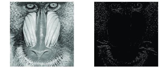
(b)

Figure 1: Illustration of the (a): Lena test, (b): mandrill test.

   1. In test Lena, we register the rotated versions of the red and green channels of image Lena, see Fig. 1(a).

   2. In the mandrill test we register the rotated versions of the gray-scale image of a mandrill baboon and its Sobel filtered version, see Fig. 1(b).

2. we chose to evaluate the objective function (1) for angles from $-10^{\circ}$ to $10^{\circ}$ by steps $0.5^{\circ}$ and in interval $[-1^{\circ},1^{\circ}]$ by steps $0.1^{\circ}$. In the ideal case the optimal degree $\theta^{*}$ is $0$. Our performance measure is the deviation from the optimal value.

In our simulations,

• we chose the $D=(2h+1)\times(2h+1)$ rectangle around each pixel as the feature $f$ of that pixel.

• coordinates of the $\mathbf{R}_{n}$ RP matrices were drawn independently from standard normal distribution, but more general constructions could also be used [33, 34].

• for each individual parameter, $10$ random runs were averaged. Our parameters included $h$, the linear size of the neighborhood that determines dimension $D$ of the feature, $G$, the size of the randomly projected groups and $d$, the dimension of RP.

• performance statistics are summarized by means of notched boxed plots, which show the quartiles ($Q_{1},Q_{2},Q_{3}$), depict the outliers, i.e., those that fall outside of interval $[Q_{1}-1.5(Q_{3}-Q_{1}),Q_{3}+1.5(Q_{3}-Q_{1})]$ by circles, and whiskers represent the largest and smallest non-outlier data points.

• we studied the efficiency of five different entropy estimating methods in (3) including

  • the recursive k-d partitioning scheme [38],

  • the $k$-nearest neighbor method [37],

  • generalized k-nearest neighbor graphs [39],

  • minimum spanning tree based entropy graphs [40, 36] and

  • the weighted nearest neighbor method [41].

  The methods will be referred to as kdp, kNN_k, kNN_1-k, MST and wkNN, respectively. kdp is a plug-in type method estimating the underlying density directly, hence especially efficient for small dimensional ($d$) problems. [39] extends the approach of [37] ($S=\{k\}$) to an arbitrary $S$ neighborhood subset ($S\subseteq\{1,\ldots,k\}$). In our experiments, we set $S=\{1,\ldots,k\}$. Instead of k-nearest graphs the total sum of pairwise distances is minimized over spanning trees in the MST method. The kNN_k, kNN_1-k, MST constructions belong to the general umbrella of quasi-additive functionals [40] providing statistically consistent estimation for the Rényi entropy ($H_{\alpha}$) [42] . The Shannon’s entropy $H$ is a special case of this family since $\lim_{\alpha\rightarrow 1}H_{\alpha}=H$. In our simulations, we chose $\alpha=0.95$. $k$, the number of neighbors in kNN_k, kNN_1-k was $5$. Finally, the wkNN technique makes use of a weighted combination of k-nearest neighbor estimators for different $k$ values.

• $h$, the neighborhood parameter was selected from the set $\{1,2,3,4,5,10,20,30\}$.

• $G$, the size of groups and $d$, the RP dimension took values $20$, $50$, $100$, $1,000$, $10,000$, $100,000$ and $1,2,5,8$, respectively.

• the $T$ feature points were distributed randomly into groups of size $G$ in order to increase the diversity of the individual groups.

In the first set of experiments we focused on the precision of the estimations on the Lena dataset. According to our experiences

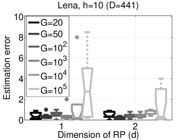
(a)

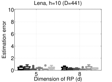
(b)

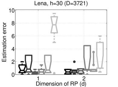
(c)

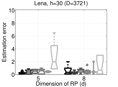
(d)

Figure 2: Estimation error as a function of the RP dimension $d$ on the Lena dataset for different $G$ group sizes. Method: kdp. (a)-(b): $h=10$. (c)-(d): $h=30$. First column: $d=1$, $2$. Second column: $d=5$, $8$.

• there is no relevant/visible difference in the precision of the estimations for $h\in\{1,2,3,4,5,10\}$. The estimation is even of high precision for $h=10$ that we illustrate in Fig. 2(a)-(b) for the kdp technique. The estimation errors are quite similar for $h=20$ and $30$, the latter is shown in Fig. 2(c)-(d). Here, one can notice a small uncertainty in the estimations for smaller RP dimensions ($d=1,2$), which is moderately present for larger $d$ values ($d=5,8$) – except for the largest studied group size $G=100,000$.

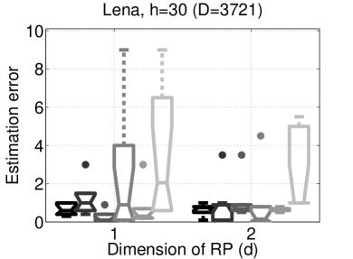
(a)

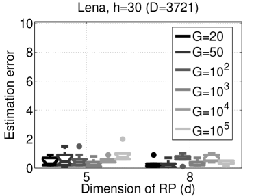
(b)

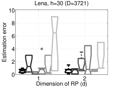
(c)

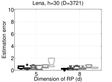
(d)

Figure 3: Estimation error as a function of the RP dimension $d$ on the Lena dataset for different $G$ group sizes. Neighbor size: $h=30$. (a)-(b): kNN_k method. (c)-(d): kNN_1-k method. First column: $d=1$, $2$. Second column: $d=5$, $8$.

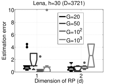
(a)

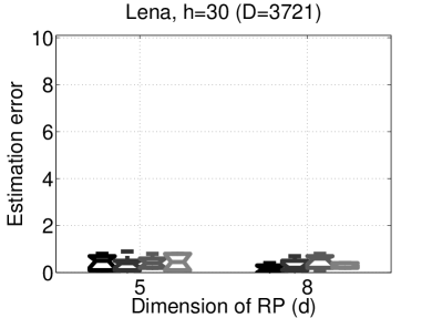
(b)

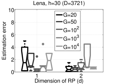
(c)

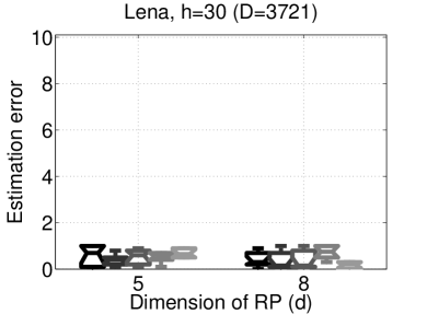
(d)

Figure 4: Estimation error as a function of the RP dimension $d$ on the Lena dataset for different $G$ group sizes. Neighbor size: $h=30$. (a)-(b): MST method. (c)-(d): wkNN method. First column: $d=1$, $2$. Second column: $d=5$, $8$.

• the obtained results are of similar precision on this dataset for all the studied entropy estimators. We illustrate this property for the most challenging $h=30$ value in Fig. 3 and Fig. 4.

In the second set of experiments we were dealing with the mandrill dataset, where different modalities of the same image (pixel, edge filtered version) had to be registered. Here,

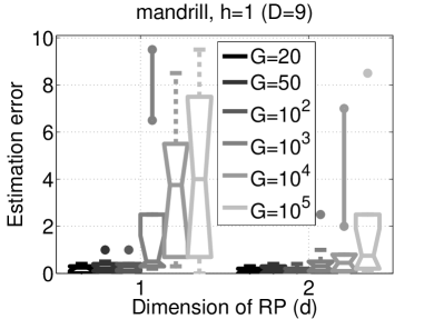
(a)

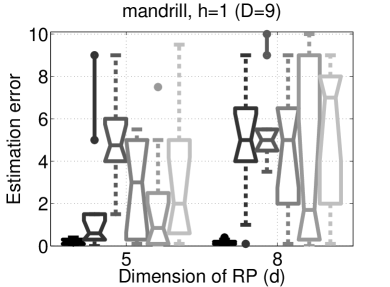
(b)

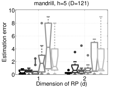
(c)

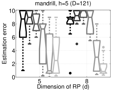
(d)

Figure 5: Estimation error as a function of the RP dimension $d$ on the mandrill dataset for different $G$ group sizes. Method: kdp. (a)-(b): neighbor size $h=1$. (c)-(d): $h=5$. First column: $d=1$, $2$. Second column: $d=5$, $8$.

• the kdp approach gradually deteriorates as the dimension of the underlying feature representation is increasing, i.e., as a function of $h$. For $h=1$, the method gives precise estimations for $d=1,2$ and small group sizes ($G=20,50,100$); other parameter choices result in uncertain estimations, see Fig. 5(a)-(b). By increasing the size of neighborhood ($h$), the estimations gradually break down. For $h=5$, the precisions are depicted in Fig. 5(c)-(d); the estimations are still acceptable. For $h=10$ we did not obtain valuable estimations for the kdp technique.

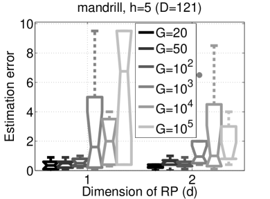
(a)

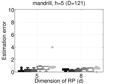
(b)

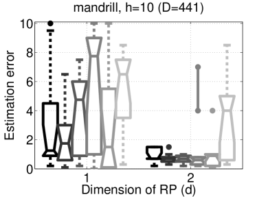
(c)

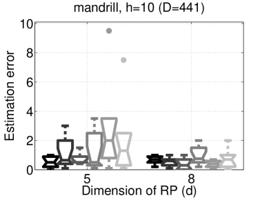
(d)

Figure 6: Estimation error as a function of the RP dimension $d$ on the mandrill dataset for different $G$ group sizes. Method: kNN_k. (a)-(b): neighbor size $h=5$. (c)-(d): $h=10$. First column: $d=1$, $2$. Second column: $d=5$, $8$.

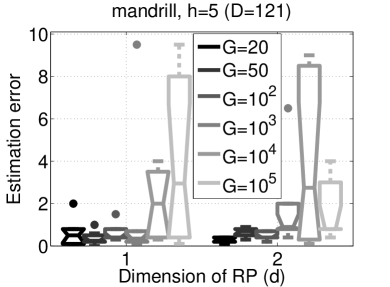
(a)

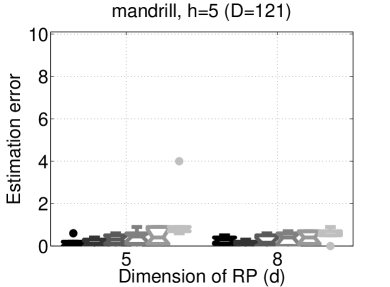
(b)

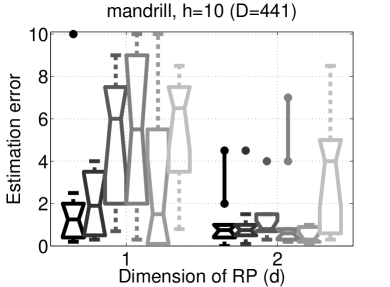
(c)

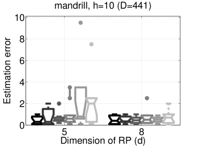
(d)

Figure 7: Estimation error as a function of the RP dimension $d$ on the mandrill dataset for different $G$ group sizes. Method: kNN_1-k. (a)-(b): neighbor size $h=5$. (c)-(d): $h=10$. First column: $d=1$, $2$. Second column: $d=5$, $8$.

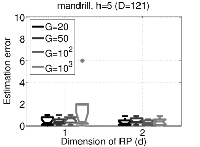
(a)

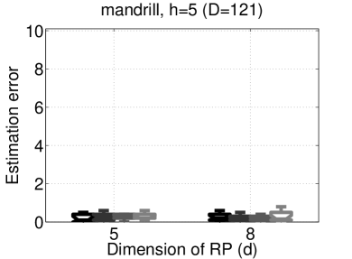
(b)

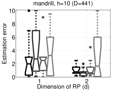
(c)

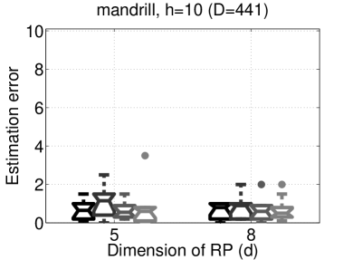
(d)

Figure 8: Estimation error as a function of the RP dimension $d$ on the mandrill dataset for different $G$ group sizes. Method: MST. (a)-(b): neighbor size $h=5$. (c)-(d): $h=10$. First column: $d=1$, $2$. Second column: $d=5$, $8$.

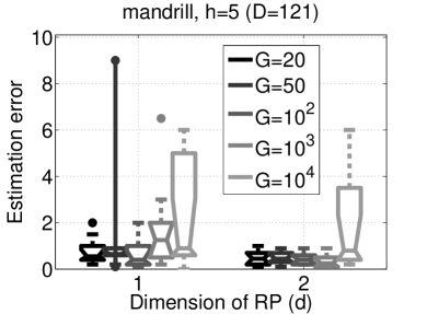
(a)

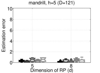
(b)

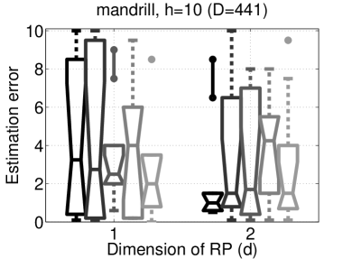
(c)

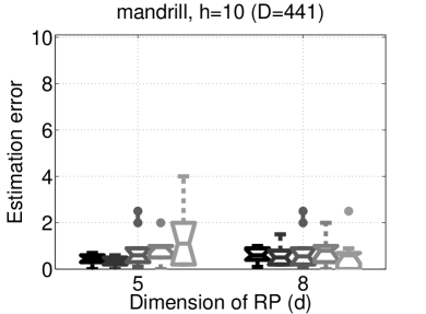
(d)

Figure 9: Estimation error as a function of the RP dimension $d$ on the mandrill dataset for different $G$ group sizes. Method: wkNN. (a)-(b): neighbor size $h=5$. (c)-(d): $h=10$. First column: $d=1$, $2$. Second column: $d=5$, $8$.

• in contrast to the kdp method, the kNN_k, kNN_1-k, MST and wkNN techniques are all capable of coping with the $h=5$ and $h=10$ values, as it is illustrated in Fig. 6, Fig. 7, Fig. 8 and Fig. 9, respectively. It can also be observed, that the RP dimension must be $d\geq 2$ here, and in case of $d=5,8$ one obtaines highly precise/certain estimations.

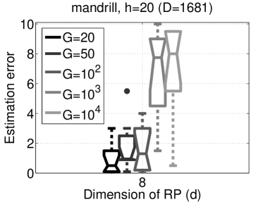
(a)

Figure 10: Estimation error for RP dimension $d=8$ and for different $G$ group sizes. Method: wkNN. Neighbor size: $h=20$.

• the only method which could cope with the increased $h=20$ neighbor size value, was the $wkNN$ technique. This result could be achieved for RP dimension $d=8$ making use of small group sizes ($G=20,50,100$), see Fig. 10.

The computation times are illustrated for the Lena ($h=30$) and mandrill dataset ($h=5$) for the kdp method in Fig.11(a) and Fig.11(b), respectively. As it can be seen, the ensemble approach with group size $G=20-100$ may speed up computations by several orders of magnitudes; similar trends can be obtained for the other estimators, too. Among the studied methods, the kdp technique was the most competitive in terms of computation time. We also present the computation times for the largest studied problem, Lena with $h=30$; compared to kdp

• the kNN_k and kNN_1-k techniques were within a factor of $1.5-2.5$ in terms of computation time,

• the wkNN method was $1.5-2$ ($3-4$) times slower compared to the kdp approach in case of $G\leq 1,000$ ($G=10,000$), and

• the MST based estimator was within a factor of $1.5-2$ compared to kdp in case of $G\leq 100$, and more than $6$ times slower for $G=1,000$.

As it can be seen in Fig. 11, the application of the reduced RP dimension can be advantageous in terms of computation time. Moreover, compared to schemes without dimensionality reduction ($d=D$ and $\mathbf{R}_{n}=\mathbf{I}$, $\forall n$), i.e., working directly on raw data, the presented RP based dimensionality approach can heavily speed-up computations. This behaviour is already present for $h=5$, as it is illustrated for $d=2$ on the mandrill dataset in Table 1.

Considering the possible $\mathbf{(h,d,G)}$ choices, according to our numerical experiences,

• often, small $d=2-5$ RP dimensions give rise to reliable estimations for several entropy methods,

• it is necessary to slowly increase $d$ as a function of the dimension of the feature representation (parameterized by $h$),

• in the studied parameter domain, group sizes of $G=50-100$ could provide precise estimations, and simultaneously open the door to massive speed-up by distributed solutions.

These results demonstrate the efficiency of our RP based approach.

5 Conclusions

We have shown that the random projection (RP) technique can be adapted to distributed information theoretical image registration. Our extensive numerical experiments including five different entropy estimators demonstrated that the proposed approach (i) can offer orders of magnitude in computation time, and (ii) provides robust estimation for large dimensional features.

It is very promising since it is parallel and fits multi-core architectures, including graphical processors. Since information theoretical measures are robust, our method may be useful in diverse signal processing areas with the advance of multi-core hardware.

About the author–ZOLTÁN SZABÓ (Applied Mathematics M.Sc. 2006, Ph.D. 2012, Informatics Ph.D. 2009) is a research fellow at the Eötvös Loránd University. In 2007, he won the Scientist of the Year Award of the Faculty of Informatics. In 2008, he obtained the Bronze Medal of the Pro Patria et Scientia Award of Hungarian Ph.D. Students. He is a reviewer at the IEEE Transactions on Neural Networks and Learning Systems, Signal, Image and Video Processing, Neurocomputing and IEEE Transactions on Signal Processing journals. His research interest include Independent Subspace Analysis and its extensions, information theory, kernel methods, group-structured dictionary learning and collaborative filtering.

About the author–ANDRÁS LŐRINCZ (Physics M.Sc. 1975, Solid State Physics Ph.D. 1978, Molecular Physics C.Sc. 1986, Laser Physics habilitation, 1998, Information Technology habilitation, 2009) is a senior researcher of Information Science at Eötvös Loránd University. He is a Fellow of the European Coordinating Committee for Artificial Intelligence. He has published more than 140 peer reviewed journal 80 peer reviewed conference papers on his research areas. He has been leading a group working on different aspects of intelligent systems.

(a)

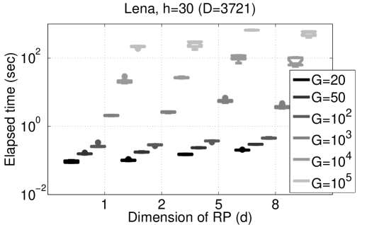
(a)

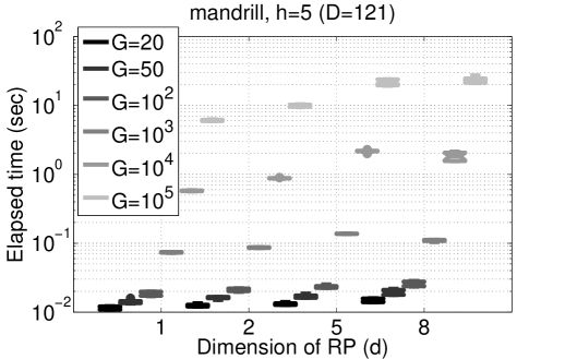
(b)

Figure 11: Computation time as a function of the RP dimension for different $G$ group sizes with log scale on the $y$ axis. Method: kdp. (a): Lena dataset, neighbor size $h=30$. (b): mandrill dataset, $h=5$.

	$G=20$	$G=50$	$G=100$	$G=1000$
kdp	$1.01$	$1.27$	$1.29$	$2.92$
kNN1-k (kNNk)	$2.25$	$5.71$	$12.65$	$125.84$
MST	$1.15$	$1.36$	$1.65$	$1.82$
wkNN	$1.30$	$2.59$	$4.88$	$16.05$

Table 1: Computation time versus raw data based method. Value $z>1$, means $z$ times improvement in computation time over the method not applying dimension reduction. Dataset: mandrill. Baseline: RP dimension $d=2$. Neighbor size: $h=5$.

References

- Fradkin and Madigan [2003] D. Fradkin, D. Madigan, Experiments with random projections for machine learning, in: International Conference on Knowledge Discovery and Data Mining (KDD 2003), pp. 517–522.
- Deegalla and Boström [2006] S. Deegalla, H. Boström, Reducing high-dimensional data by principal component analysis vs. random projection for nearest neighbor classification, in: International Conference on Machine Learning and Applications (ICMLA 2006), pp. 245–250.
- Goel et al. [????] N. Goel, G. Bebis, A. V. Nefian, Face recognition experiments with random projections, in: SPIE Conference on Biometric Technology for Human Identification, 2005, volume 5779, pp. 426–437.
- Fern and Brodley [2003] X. Z. Fern, C. E. Brodley, Random projection for high dimensional data clustering: A cluster ensemble approach, in: International Conference on Machine Learning (ICML-2003), pp. 186–193.
- Szabó and Lőrincz [2009] Z. Szabó, A. Lőrincz, Fast parallel estimation of high dimensional information theoretical quantities with low dimensional random projection ensembles, in: Independent Component Analysis and Signal Separation (ICA 2009), volume 5441 of Lecture Notes in Computer Science, Springer-Verlag, Berlin Heidelberg, 2009, pp. 146–153.
- Ailon and Chazelle [????] N. Ailon, B. Chazelle, Approximate nearest neighbors and the fast Johnson-Lindenstrauss transform, in: Annual ACM Symposium on Theory of Computing, 2006, pp. 557 – 563.
- Hegde et al. [????] C. Hegde, M. B. Wakin, R. G. Baraniuk, Random projections for manifold learning, in: Neural Information Processing Systems (NIPS 2007), pp. 641–648.
- Mahmoudi et al. [2008] M. Mahmoudi, P. Vandergheynst, M. Sorci, On the estimation of geodesic paths on sampled manifolds under random projections, in: International Conference on Image Processing (ICIP-2008), pp. 1840–1843.
- Dasgupta [2000] S. Dasgupta, Experiments with random projection, in: Conference on Uncertainty in Artificial Intelligence (UAI-2000), Morgan Kaufmann Publishers Inc., San Francisco, CA, USA, 2000, pp. 143–151.
- Bingham and Mannila [2001] E. Bingham, H. Mannila, Random projection in dimensionality reduction: applications to image and text data, in: International Conference on Knowledge Discovery and Data Mining (KDD 2001), pp. 245–250.
- Li et al. [2007] P. Li, T. J. Hastie, K. W. Church, Nonlinear estimators and tail bounds for dimension reduction in using Cauchy random projections, Journal of Machine Learning Research 8 (2007) 2497–2532.
- Menon et al. [2007] A. K. Menon, A. Pham, S. Chawla, A. Viglas, An incremental data-stream sketch using sparse random projections, in: SIAM International Conference on Data Mining (SDM 2007), pp. 563–568.
- Lukos̆evic̆ius and Jaeger [2009] M. Lukos̆evic̆ius, H. Jaeger, Reservoir computing approaches to recurrent neural network training, Computer Science Review 3 (2009) 127–149.
- Vempala [2005] S. S. Vempala, The Random Projection Method (DIMACS Series in Discrete Math), volume 65, 2005.
- Baraniuk et al. [2008] R. Baraniuk, M. Davenport, R. DeVore, M. Wakin, A simple proof of the restricted isometry property for random matrices, Constructive Approximation 28 (2008) 253–263.
- Özuysal et al. [2010] M. Özuysal, M. Calonder, V. Lepetit, P. Fua, Fast keypoint recognition using random ferns, IEEE Transactions on Pattern Analysis and Machine Intelligence 32 (2010) 448–461.
- Kokiopoulou et al. [2009] E. Kokiopoulou, D. Kressner, P. Frossard, Optimal image alignment with random measurements, in: European Signal Processing Conference (EUSIPCO 2009), pp. 1304–1308.
- Akselrod-Ballin et al. [2009] A. Akselrod-Ballin, D. Bock, R. C. Reid, S. K. Warfield, Accelerating feature based registration using the Johnson-Lindenstrauss lemma, in: Medical Image Computing and Computer-Assisted Intervention (MICCAI 2009), volume 5761 of Lecture Notes in Computer Science, Springer, 2009, pp. 632–639.
- Healy and Rohde [2007] D. M. Healy, G. K. Rohde, Fast global image registration using random projections, in: International Symposium on Biomedical Imaging (ISBI 2007), pp. 476–479.
- Neemuchwala et al. [2007] H. Neemuchwala, A. Hero, S. Zabuawala, P. Carson, Image registration methods in high dimensional space, International Journal of Imaging Systems and Technology 16 (2007) 130–145.
- Kybic [2004] J. Kybic, High-dimensional mutual information estimation for image registration, in: IEEE International Conference on Image Processing (ICIP’04), IEEE Computer Society, 2004, pp. 1779–1782.
- Bardera et al. [2006] A. Bardera, M. Feixas, I. Boada, M. Sbert, High-dimensional normalized mutual information for image registration using random lines, in: Third International Workshop on Biomedical Image Registration (WBIR 2006), volume 4057 of Lecture Notes in Computer Science, Springer-Verlag, Berlin Heidelberg, 2006, pp. 264–271.
- Arya et al. [1998] S. Arya, D. M. Mount, N. S. Netanyahu, R. Silverman, A. Y. Wu, An optimal algorithm for approximate nearest neighbor searching in fixed dimensions, Journal of the ACM (JACM) 45 (1998) 891 – 923.
- Cardoso [1998] J. Cardoso, Multidimensional independent component analysis, in: International Conference on Acoustics, Speech, and Signal Processing (ICASSP ’98), volume 4, pp. 1941–1944.
- Szabó et al. [2007] Z. Szabó, B. Póczos, A. Lőrincz, Undercomplete blind subspace deconvolution, Journal of Machine Learning Research 8 (2007) 1063–1095.
- García-Arteaga and Kybic [2008] J. D. García-Arteaga, J. Kybic, Regional image similarity criteria based on the Kozachenko-Leonenko entropy estimator, in: Computer Vision and Pattern Recognition Workshops (CVPRW-2008), pp. 1–8.
- Cover and Thomas [1991] T. M. Cover, J. A. Thomas, Elements of information theory, John Wiley and Sons, New York, USA, 1991.
- Johnson and Lindenstrauss [1984] W. B. Johnson, J. Lindenstrauss, Extensions of Lipschitz maps into a Hilbert space, Contemporary Mathematics 26 (1984) 189–206.
- Frankl and Maehara [1987] P. Frankl, H. Maehara, The Johnson-Lindenstrauss Lemma and the sphericity of some graphs, Journal of Combinatorial Theory Series A 44 (1987) 355 – 362.
- Indyk and Motwani [????] P. Indyk, R. Motwani, Approximate nearest neighbors: Towards removing the curse of dimensionality, in: ACM Symposium on Theory of Computing, 1998, pp. 604–613.
- Achlioptas [2003] D. Achlioptas, Database-friendly random projections: Johnson-Lindenstrauss with binary coins, Journal of Computer and System Sciences 66 (2003) 671–687.
- Li et al. [2006] P. Li, T. J. Hastie, K. W. Hastie, Very sparse random projections, in: International Conference on Knowledge Discovery and Data Mining (KDD-2006), ACM, New York, NY, USA, 2006, pp. 287–296.
- Arriga and Vempala [2006] R. I. Arriga, S. Vempala, An algorithmic theory of learning: Robust concepts and random projections, Machine Learning 63 (2006) 161–182.
- Matous̆ek [2008] J. Matous̆ek, On variants of the Johnson-Lindenstrauss lemma, Random Structures and Algorithms 33 (2008) 142–156.
- Kozachenko and Leonenko [1987] L. F. Kozachenko, N. N. Leonenko, On statistical estimation of entropy of random vector, Problems of Information Transmission 23 (1987) 95–101.
- Hero et al. [2002] A. Hero, B. Ma, O. Michel, J. Gorman, Applications of entropic spanning graphs, Signal Processing 19 (2002) 85–95.
- Leonenko et al. [2008] N. Leonenko, L. Pronzato, V. Savani, A class of Rényi information estimators for multidimensional densities, Annals of Statistics 36 (2008) 2153–2182.
- Stowell and Plumbley [2009] D. Stowell, M. D. Plumbley, Fast multidimensional entropy estimation by k-d partitioning, IEEE Signal Processing Letters 16 (2009) 537–540.
- Pál et al. [????] D. Pál, B. Póczos, C. Szepesvári, Estimation of Rényi entropy and mutual information based on generalized nearest-neighbor graphs, in: Neural Information Processing Systems (NIPS-2010), pp. 1849–1857.
- Yukich [1998] J. E. Yukich, Probability Theory of Classical Euclidean Optimization Problems, Springer, 1998.
- Sricharan and Hero [????] K. Sricharan, A. O. Hero, Weighted k-NN graphs for Rényi entropy estimation in high dimensions, in: IEEE Workshop on Statistical Signal Processing (SSP-2011), pp. 773–776.
- Rényi [????] A. Rényi, On measures of entropy and information, in: Proceedings of the Fourth Berkeley Symposium on Mathematical Statistics and Probability, 1961, volume 1, pp. 547–561.