Hall effect in heavy-fermion metals

Abstract

The heavy fermion systems present a unique platform in which strong electronic correlations give rise to a host of novel, and often competing, electronic and magnetic ground states. Amongst a number of potential experimental tools at our disposal, measurements of the Hall effect have emerged as a particularly important one in discerning the nature and evolution of the Fermi surfaces of these enigmatic metals. In this article, we present a comprehensive review of Hall effect measurements in the heavy-fermion materials, and examine the success it has had in contributing to our current understanding of strongly correlated matter. Particular emphasis is placed on its utility in the investigation of quantum critical phenomena which are thought to drive many of the exotic electronic ground states in these systems. This is achieved by the description of measurements of the Hall effect across the putative zero-temperature instability in the archetypal heavy-fermion metal YbRh₂Si₂. Using the Ce$M$In₅ (with $M=$ Co, Ir) family of systems as a paradigm, the influence of (antiferro-)magnetic fluctuations on the Hall effect is also illustrated. This is compared to prior Hall effect measurements in the cuprates and other strongly correlated systems to emphasize on the generality of the unusual magnetotransport in materials with non-Fermi liquid behavior.

	Contents	Page
1.	Introduction	1
	1.1.  Significance of Hall effect to heavy-fermion systems	1.1
	1.2.  Contemporary issues in heavy-fermion systems	1.2
	1.3.  Classification of quantum critical points via Hall effect	1.3
	1.4.  Outline and scope	1.4
2.	Basics of Hall effect and heavy-fermion systems	2
	2.1.  History of the Hall effect	2.1
	2.2.  The influence of magnetism: Anomalous Hall effect	2.2
	2.3.  Mechanisms contributing to the anomalous Hall effect	2.3
	2.3.1.  Skew scattering	2.3.1
	2.3.2.  Side-jump mechanism	2.3.2
	2.3.3.  Berry phase contributions	2.3.3

		Page
	2.4.  Hall effect and Fermi surface	2.4
	2.5.  Basic remarks on heavy-fermion systems	2.5
	2.6.  Anomalous Hall effect in heavy-fermion systems	2.6
3.	Theoretical work on the Hall effect	3
	3.1.  Theoretical Overview	3.1
	3.2.  Key results from Boltzmann theory	3.2
	3.3.  Hall effect within Fermi liquid theory	3.3
	3.4.  Quantum critical heavy fermion metals	3.4
	3.4.1.  “Conventional” Hertz-Moriya-Millis quantum
	criticality	3.4.1
	3.4.2.  Spin-fluctuation theory	3.4.2
	3.5.  Hall effect across Kondo breakdown quantum critical point	3.5
	3.5.1.  Quantum criticality in heavy fermion metals and
	jump of Hall coefficient	3.5.1
	3.5.2.  Crossover and scaling of the Hall coefficient at $T\neq 0$	3.5.2
4.	Experimental aspects of Hall effect measurements in metals	4
	4.1.  Measurement techniques	4.1
	4.2.  Advanced aspects of Hall effect measurements	4.2
	4.2.1.  Single-field Hall experiments	4.2.1
	4.2.2.  Crossed-field Hall experiments	4.2.2
	4.2.3.  Realization of crossed-field Hall experiments	4.2.3
	4.2.4.  Comparing single and crossed-field Hall experiments	4.2.4
5.	Hall effect and Kondo-breakdown quantum criticality	5
	5.1.  Hall effect evolution at the QCP in YbRh2Si2	5.1
	5.2.  Comparison to other candidates for Kondo breakdown	5.2
	5.3.  Hall effect and scaling behavior	5.3
6.	Hall effect in systems with 115 type of structure	6
	6.1.  Influence of magnetic fluctuations on superconductivity	6.1
	6.2.  Interplay magnetism and superconductivity in Ce$M$In5	6.2
	6.3.  Hall effect measurements on Ce$M$In5 systems	6.3
	6.3.1.  Scaling relations in Hall effect	6.3.1
	6.3.2.  CeCoIn5	6.3.2
	6.3.3.  CeIrIn5	6.3.3
	6.3.4.  Comparative remarks	6.3.4
7.	Comparison to Hall effect of other correlated materials	7
	7.1.  Copper oxide superconductors and related systems	7.1
	7.1.1.  Cuprates	7.1.1
	7.1.2.  Comparison of cuprates and heavy-fermion systems	7.1.2
	7.1.3.  Hall effect in oxy-pnictides and related systems	7.1.3
	7.2.  Other systems of related interest	7.2
	7.3.  Colossal magnetoresistive manganites	7.3
8.	Summary	8
9.	Appendix	9
	Acknowledgement	Acknowledgments
	References	Acknowledgments

1 Introduction

1.1 Significance of Hall effect in heavy-fermion systems

The heavy fermion metals represent an enigmatic class of strongly correlated electron systems, in which the strong hybridization between the conduction electrons and localized $f$ moments results in a Landau Fermi liquid (LFL) at low temperatures with heavily renormalized quasiparticle properties [1]. A dramatic manifestation of the strong many body effects in these systems was uncovered in 1979 with the discovery of superconductivity in CeCu₂Si₂ [2]. Predating the flurry of activity in the high temperature superconducting cuprates, this represented the first observation of superconductivity in an inherently magnetic environment. It was followed by the observation of superconductivity in many heavy fermion metals [3]. It has also motivated the search for electronic (more specifically, magnetic) mechanisms for superconducting pairing. The resurgence of research into the heavy fermion metals is primarily due to current interest in continuous quantum phase transitions—a zero-temperature instability which can be tuned by the use of a non-thermal control parameter [4, 5, 6]. The presence of such a zero-temperature instability is often manifested in a large region of the experimentally accessible phase space, as has been clearly demonstrated in many systems. The celebrated Landau-Fermi-liquid theory of conventional metals breaks down in the vicinity of such instabilities [5], and anomalous experimental behavior like a linear temperature dependence of the electrical resistivity [7], a non-saturating specific heat coefficient [8] and an apparent violation of the Wiedemann-Franz law [9, 10] have been observed. This instability also appears to be linked to the emergence of novel states of matter—for example superconductivity (as mentioned above) is often observed in the vicinity of a quantum phase transition [11]. A related development has been the growing realization that the physics of the heavy-fermion systems and the high-temperature superconducting cuprates have much in common. What makes this so fascinating is that unlike the heavy fermions metals, the parent high-transition-temperature (high-$T_{\rm c}$) superconductors are Mott insulators. In this context it is surprising that the superconducting and normal state properties of some heavy fermion systems are so similar to the high-$T_{\rm c}$ cuprates [12].

A microscopic explanation of the physics of the heavy-fermion systems calls for an understanding of how the Fermi surfaces of these complex systems evolve as a function of various experimental control parameters. Measurements of the de Haas–van Alphen (dHvA) effect and of angle resolved photo electron spectroscopy (ARPES) are amongst the most powerful tools for this purpose. In particular, dHvA effect measurements demonstrated [13] the applicability of a description by strongly renormalized quasiparticles in UPt₃. In general, however, extreme sensitivity to disorder along with prerequisites of very low temperatures and high fields have limited the application of these techniques to the heavy-fermion systems. It is in this context that measurements of the Hall effect [14]—a relatively simpler experimental technique—has proven illuminating. This is in spite of the fact that the Hall effect itself is a complex quantity, especially in systems like the heavy-fermion systems which usually have more than one band crossing the Fermi level. Moreover, the contribution from the anomalous Hall effect which results from skew scattering [15], is an important factor in materials comprised of an array of localized magnetic moments. However, it has been shown that at low temperatures the contribution from skew scattering is negligible in the heavy-fermion systems [16], and thus the experimentally measured Hall voltage predominantly arises from the normal part of the Hall effect. Consequently, at these temperatures the Hall effect can provide a crucial—albeit indirect—measure of the Fermi surface volume.

Measurements of the Hall effect have also been extremely useful in revealing the normal-state properties of heavy-fermion superconductors. For instance, the possible presence of a pseudogap-like precursor state to superconductivity in Ce$M$In₅ system ($M$ = Co, Ir) has been proposed. Comparison with prior results on the Hall effect in the superconducting cuprates reveals many striking similarities, indicating that the non-Fermi-liquid physics probably affect the Fermi surfaces of these diverse materials in a rather similar fashion. An anisotropic reconstruction of the Fermi surface by the formation of “hot” and “cold” regions with different scattering rates has been suggested, which then manifests itself in the form of two distinct scattering times that influence the resistivity and Hall effect in these materials in disparate manners [17, 18]. Recent measurements of the Hall effect in cuprates have reinforced its utility in uncovering the relation between quantum magnetism and superconductivity in these complex materials [19, 20, 21].

The theory of the Hall effect in strongly correlated systems remains an exceedingly difficult problem, in part due to the acute sensitivity of the Hall response to the constitution and topology of the Fermi surface. Earlier calculations on metals relied on approximating the Fermi surface to simple geometric constructions without taking into account the specific band structure of the materials under consideration [22, 23]. Unusual Hall behavior in the cuprates [24] triggered intense activity in this area, and besides a more generic geometric treatment [25], models like the nearly antiferromagnetic Fermi liquid [26] and the spin-charge separation [27] scenario, and others were employed to account for the experimental observations. For the heavy-fermion metals, the Hall constant was predicted to allow for a qualitative distinction between different scenarios for quantum criticality [28]. The Hall effect and the resistivity have also been calculated using current vertex corrections (CVC) on a Fermi liquid in the presence of antiferromagnetic fluctuations, in an attempt to unify observations in the cuprates and the heavy-fermion metals [29].

1.2 Contemporary issues in heavy-fermion systems

The recent interest in heavy-fermion systems stems from their model character in the investigation of quantum critical points. Although occurring at zero temperature, a quantum critical point (QCP) may lead to unusual properties up to surprisingly high temperatures. We shall see that the Hall effect is a sensitive tool to explore the nature of a QCP.

Two main approaches are available to describe QCPs in heavy fermion metals (cf. Fig. 1). Conventionally, the order parameter notation is generalized by incorporating quantum corrections. For the heavy-fermion systems magnetism is treated itinerantly giving rise to a spin-density wave (SDW) [4, 30, 31]. This approach relies on the fact that the composite quasiparticles formed by the Kondo effect stay intact at the quantum critical point, Fig. 1(a).

By contrast, more recent studies additionally incorporate quantum modes to become critical [32, 33]. In the case of the heavy-fermion systems the critical quantum modes are associated with the Kondo effect. When the Kondo effect becomes critical, the quasiparticles disintegrate at the QCP, Fig. 1(b). As a consequence, the Fermi surface is expected to jump at such an unconventional QCP. This is to be contrasted with the conventional QCP for which a continuous evolution of the Fermi surface is expected. Hence, the evolution of the Fermi surface is a fundamental feature distinguishing the Kondo breakdown from the SDW scenario. In fact, Hall effect measurements were suggested to characterize QCPs [28]. The second fundamental difference between the two scenarios is their scaling behavior. For the 3D SDW QCP an $E/T^{3/2}$ scaling is predicted for the spin dynamics, whereas an $E/T$ scaling is expected at a Kondo breakdown QCP. The first example for an unconventional QCP was identified in CeCu_6-xAu_x by observation of an $E/T$ scaling in inelastic neutron scattering measurements [34]. This Kondo breakdown scenario will be further discussed in section 3.5.2. In the following we shall see how Hall effect

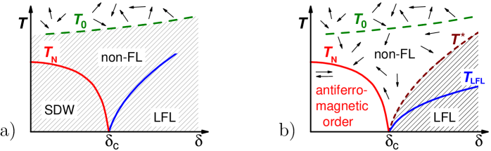
Figure 1: Comparison of quantum criticality in a) the spin-density wave (SDW) and b) the locally critical scenario. $\delta$ refers to an external control parameter for tuning the material to its QCP at $\delta_{c}$. The hatched areas indicate phase space regions within which the heavy quasi-particles are formed, whereas the arrows illustrate the existence of local magnetic moments. In the local scenario (b) the quasi-particles themselves break apart at $\delta_{c}$. At finite temperatures the quasiparticles disintegrate within a crossover range indicated by the $T^{*}$ line. $T_{\mathrm{LFL}}$ marks the temperature below which LFL behavior is found, whereas $T_{0}$ denotes the onset temperature for initial Kondo screening.

measurements may shed light on the dynamics and on the scaling behavior.

1.3 Classification of quantum critical points via Hall effect

Hall effect measurements currently provide the best probe to study the Fermi surface evolution at QCPs. This is mainly due to the experimental difficulties associated with other probes: Photo electron spectroscopy on the one hand is—in the context discussed here—limited to relatively high temperatures and moderate energy resolution ($\Delta E$ in the order of meV). Quantum oscillation measurements, on the other hand, can only be conducted in high magnetic fields which are often beyond interesting energy scales, and require clean samples which often excludes the investigation of composition-driven QCPs.

In order to distinguish whether the Fermi surface evolves continuously or discontinuously one needs to have sufficient resolution of the control parameter used to access the QCP. Widely employed tuning parameters in heavy fermion systems are pressure, composition, and magnetic field. So far, however, only magnetic field-tuned QCPs appear to allow the high resolution required.

The QCP in CeCu_6-xAu_x is tuned either by variation of gold content or by the application of pressure. Probing a pressure- or composition-driven QCP with sufficient resolution was not yet able to show an abrupt Fermi surface change in this system by means of Hall effect measurements. The critical gold concentration of $x_{\mathrm{c}}=0.1$ implies that a considerable amount of scatterers are present which change the Hall effect dramatically [35, 36]. The latter appear to lead to a dominance of the anomalous contributions to the Hall resistivity for all non-stoichiometric samples. Consequently, the normal contributions cannot be determined reliably and hence, information on the Fermi surface evolution is difficult to extract. This is also seen from the fact that no signatures are seen in the Hall resistivity when probing the field-induced QCP in samples on the magnetically ordered side of the QCP [37].

Pressure reverses the effect of Au substitution in CeCu_6-xAu_x. Consequently, the pressure-driven QCP is only accessible for samples with finite Au content. A Hall effect study on such a sample would presumably suffer from the strong anomalous contributions [38, 36]. Moreover, Hall effect studies under pressure are highly demanding. The fine tuning of pressure required to resolve a rapid change in the Fermi surface is rarely achieved. This is seen for instance in the heavy fermion system CeRh₂Si₂ where the Hall coefficient was extracted as a function of pressure [39]. The few data points obtained in the pressure range up to 1.3 GPa provide only limited insight. Here, the Hall coefficient seems to be sensitive to a change in the magnetic structure at 0.6 GPa. At the low temperature magnetic transition, however, the data appear to evolve smoothly despite the fact that de Haas–van Alphen measurements indicate a strong Fermi surface reconstruction [40]. It would be necessary to collect further data to draw a firm conclusion about the evolution of the Fermi surface. We note that the sign change of $R_{\text{H}}$ observed in proximity to the critical pressure cannot directly be related to a severe Fermi surface change since CeRh₂Si₂ features multiple bands [40], cf. discussion in section 2.4.

For the material CeRhIn₅ a drastic change of the Fermi surface at a critical pressure of about 2.3 GPa was observed by de Haas–van Alphen measurements [41] which has been ascribed to a breakdown of the Kondo effect at an underlying QCP [42]. It is to be expected that the Hall coefficient will correspondingly show a drastic change across the critical pressure. Existing Hall measurements within the zero-field limit and at relatively high temperatures (above 2 K) have already revealed a rapid change of the Hall coefficient across the critical pressure; this rapid change is likely associated with both the Kondo physics and the QCP, because it is absent in both LaRhIn₅ and CeCoIn₅ [12]. In order to determine the precise nature of the evolution of the Hall effect across the critical pressure, it is important to carry out measurements at low temperatures (0.4 K or below, where the electrical resistivity shows a $T^{2}$ dependence [43]) and at magnetic fields where superconductivity is suppressed. It should also be stressed that the precise evolution of the Hall coefficient across the QCP needs to be studied with care, given the discrete steps in pressure used as the control parameter.

A canonical SDW QCP is realized in pure and V-doped Cr [44]. Hall effect measurements under pressure conducted on these materials represent the rare examples where the Hall coefficient was measured for a large series of pressure points [45, 46], see Fig. 2. These measurements were conducted at 5 and 0.5 K, respectively, i.e. at temperatures which are small compared to the natural temperature scales of these systems. The measurements reveal a smooth crossover of the Fermi surface when the magnetic order is suppressed, a behavior which is expected theoretically [28, 47, 48]. The Fermi surface of a SDW state is reconstructed from that of the paramagnetic state through a band folding, which is more pronounced for systems like Cr whose Fermi surfaces are nested. However, if the SDW order parameter is adiabatically switched off the folded Fermi surface is smoothly connected to the paramagnetic one. As a result, the Hall coefficient does not show a jump as long as the nesting is not perfect [48]. So far, no information was extracted regarding how this crossover evolves with temperature; it would be

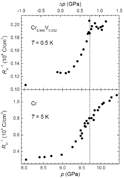
Figure 2: Inverse Hall coefficient of pure Cr (lower panel) and Cr_0.968V_0.032 (upper panel) as a function of pressure. In the upper panel, $\Delta p$ denotes the external pressure for Cr_0.968V_0.032, or an effective pressure for samples in which the V-concentration is different from 0.032 [46]. In the lower panel, the result is shown only in the vicinity of the critical pressure [45] so that the two panels cover the same pressure extent. The dashed lines label the critical pressure. Reproduced with permission from S. Friedemann et al., Journal of Physics: Condensed Matter 23 (2011) 094216 [49]. Copyright (2011) IOP Publishing Ltd.

interesting to see if the finite crossover width persists in the extrapolation to zero temperature as expected for a SDW scenario. However, we wish to point out that these pressure measurements were very extensive and it would be an even larger effort to implement the techniques used to the low temperatures needed to study heavy fermion systems.

The remaining common tuning parameter, magnetic field, appears to be the obvious choice to achieve high resolution. In case of a magnetic-field driven QCP, however, the non-zero critical field can give rise to a small discontinuity in the magnetotransport coefficients even in the case of an SDW QCP [50]. Approaching the QCP, the energy scale associated with the vanishing order parameter becomes smaller than the scale associated with the Lorentz force, leading to a non-linearity in the system’s response to the Lorentz force. This is reflected in a breakdown of the weak-field magnetotransport. The linear field dependence of the magnetoresistance in Ca₃Ru₂O₇ was taken as indication thereof [51]. Moreover, the breakdown of weak-field magnetotransport may lead to a jump in the Hall coefficient which, however, is likely to be very small. In fact, for the case of the cuprates mean field theory predicts that the anomaly in the Hall response at the critical doping level is negligibly small even though the SDW gap is large [52]. Disorder may smear the jump of the Hall coefficient into a smooth crossover.

For the above-mentioned pressure-driven SDW QCP of pure and V-doped Cr [46, 45], the Hall coefficient (and the resistivity) exhibits a smooth crossover near the QCP the width of which does not track the strength of disorder (Fig. 2). This behaviour is in contrast to the scenario of a breakdown of the weak-field limit. For the field-driven QCP of YbRh₂Si₂, the effect of non-linear response to the Lorentz force is expected to be negligible, given that at the critical field, $\omega_{c}\tau$ as defined in eq. (3) is very small (on the order of 0.01 and 0.002 for the samples described in Ref. [53]). Furthermore, it is completely avoided by the crossed-field Hall setup, see section 4.2.2.

1.4 Outline and Scope

In this article, we give an overview of experimental and theoretical work on the Hall effect in the heavy fermion metals. We start with a brief description of the basics of the Hall effect, and an introduction to the anomalous Hall effect in section 2. Subsequently, we introduce the heavy-fermion metals and describe the ingredients which go into the formation of the heavy-fermion fluid. A description of the anomalous Hall effect is carried over from the earlier section, and a more microscopic description of this effect is provided. The relevance of Hall effect measurements in the investigation of these systems is stated, and the use of the Hall effect in identifying some transitions and crossovers observed in the low-temperature phase diagrams of the heavy-fermion systems is described. Section 3 provides an account of theoretical work on the Hall effect in strongly correlated electron systems. This incorporates models ranging from the earlier geometric methods to contemporary ones where the details of band structure are explicitly considered. A brief description of the experimental aspects of Hall effect measurements are provided in section 4. Special mention is made of the crossed-field Hall experiments, where a tuning field is introduced in addition to the magnetic field used for generating the Hall response. The influence of strong magnetic fluctuations on the physical properties of the heavy-fermion systems is well documented. Section 6 describes the signatures of these magnetic fluctuations as seen in Hall effect measurements. Special mention will be made of the Ce$M$In₅ ($M$ = Co, Ir or Rh) family of compounds where a complex interplay between superconductivity and magnetism has been observed. Section 5 deals with the investigation of quantum critical phenomena – a topic of contemporary interest. The utility of Hall effect measurements in the investigation of quantum criticality will be outlined, and experimental work in this area is reviewed. In section 7, we compare the Hall effect in the heavy-fermion systems with observations in other strongly correlated electron systems, with emphasis on the manganites, doped Mott insulators and the copper oxide superconductors. Section 8 sets out some open questions.

One cannot hope to be comprehensive in this vast subject, so we have omitted several issues entirely. These include the heavy-fermion transition metal oxides as well as the mixed state of the heavy-fermion superconductors. Since only a very brief description on early work in metals is included in section 2, we refer the reader to earlier reviews [54, 14, 55] which deal exclusively with the Hall effect in metals and alloys.

2 Basics of Hall effect and heavy-fermion systems

2.1 History of the Hall effect

Unconvinced by a passage from Maxwell’s treatise on Electricity and Magnetism which stated that “the path of a current through a conductor is not permanently altered by a magnetic field”, Edwin H. Hall, in 1879, set about investigating the action which a magnetic field would have on such a current. Using experiments on a gold leaf held between the poles of an electromagnet, he observed that when a magnetic field is applied perpendicular to the direction of a current flow, an electric field is generated perpendicular to both, the direction of the current, and the direction of the magnetic field [56]. This resultant electric field could then be detected using a sensitive galvanometer. Hall also realized that the product of the current through the specimen and the strength of the magnetic field, when divided by the current through the galvanometer, was reasonably constant. In current notation, this implies that $V_{\rm H}\propto BI$, where $B$ and $I$ refer to the magnetic flux density and the current flowing through the specimen, respectively, and $V_{\rm H}$ denotes the transverse (Hall) voltage.

Intuitively, this can be seen as a direct consequence of the Lorentz force acting on the electron current flowing through the solid. Consider a rectangular specimen of width $b$ and height $d$ as shown in Fig. 3 and assume a current $I_{x}$ of charge carriers $q$ with density $n$ flowing uniformly along its length with velocity $v_{x}$. When $B_{z}$ is applied perpendicular to the direction of the current, the electrons are deflected by the Lorentz force towards the edge of the specimen. This transient motion builds up a charge at (and thus an electric field $E_{y}\equiv E_{\rm H}$ between) the edges of the sample, which in turn impedes further electrons from accumulating at the edges. A stationary state is achieved when the deflection of charge carriers due to the Lorentz force is balanced by the force resulting from the transverse electric field: $E_{\rm H}-(v_{x}B_{z})=0$. With $I_{x}/bd=nqv_{x}$ one finds for the Hall voltage $V_{y}=E_{\rm H}/b$ within the simple free electron model:

$$V_{y}=\frac{1}{nq}\frac{I_{x}}{d}B_{z}=R_{\rm H}\frac{I_{x}}{d}B_{z}$$ (1)

The constant of proportionality $R_{\rm H}=1/nq$ is the so-called Hall coefficient. Obviously, Hall measurements can reveal information on the type of charge carriers. This was soon realized with the observation of a positive $R_{H}$ in some metals. Eq. (1), however, is strictly valid only if the material can be described by a simple one-band picture. In more complex materials, more then one band may exist at the Fermi energy $E_{F}$ and hence, contributes to the conductivity. In these

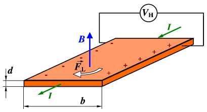
Figure 3: Schematic setup for the measurement of the Hall effect.

cases, the charge carrier concentration as determined from Hall measurements has to be considered an effective one, $n_{\rm eff}$, and the interpretation of the results can be considerably complicated, see e.g. [14] and section 2.4.

2.2 The influence of magnetism: Anomalous Hall effect

The Hall effect in metals is a direct consequence of the breaking of time reversal symmetry, in this case by the application of an external magnetic field $H$. It was realized very early on that the Hall effect could possibly arise even in the absence of an external field, as long as time reversal symmetry is broken. Early experimental insight was provided by measurements on ferromagnetic elements and alloys, where unlike that observed in simple diamagnetic metals, a pronounced nonlinearity in the field dependence of the Hall signal was observed [57, 58, 59] (paramagnetic materials may exhibit small nonlinearities). The Hall voltage was not only seen to be proportional to the magnetization $M$, but also appeared to reproduce the irreversibilities observed in the magnetization curves [60, 61, 62]. This additional contribution to the ordinary, or normal, Hall effect was termed the extraordinary, or anomalous, Hall effect (AHE). At fields larger than that required to drive the magnetization of the material into saturation, the Hall effect continued to increase, albeit at a much slower rate.

Empirically, the measured Hall resistivity in ferromagnets could thus be written as

$$\varrho_{xy}=R_{\rm 0}B+R_{\rm S}\mu_{0}M$$ (2)

where $R_{0}$ and $R_{S}$ refer to the normal and the anomalous Hall effect contributions, respectively. Fig. 4 shows a schematic of the typical behavior of the Hall resistivity in a metal with appreciable magnetization as a function of applied field. Two distinct, linear regimes with different slopes are clearly discernible. In the first one, the slope equals $R_{0}+R_{\rm S}$. The second regime lies above the technical saturation field, and here the smaller slope corresponds to $R_{0}$ only. The straight extrapolations of these two regimes intersect at $B=\mu_{0}M_{S}$ where $M_{S}$ is the spontaneous magnetization. Though the empirical formula (2) assumes that the anomalous Hall effect is directly proportional to the magnetization, the observed phenomenon could not be simply explained in terms of the internal field of the ferromagnetic system. A non-trivial temperature dependence and even a change of sign of the Hall signal at low temperature in some systems, warranted the use of more sophisticated models to explain the experimental data (see, e.g., Ref. [63]). It is now understood that the extent and dependencies of the AHE arise as a consequence of the spin-orbit coupling, although some of the microscopic details continue to remain investigated. In what follows three basic mechanisms which have been used to account for the anomalous Hall effect, namely “skew scattering”, the “side-jump” mechanism and the “Berry phase” induced Hall signal, are described in more detail. For early reviews of the anomalous Hall effect, the reader is referred to Refs. [14, 64] whereas more contemporary reviews on the anomalous Hall effect are provided in Refs. [65, 66, 67].

2.3 Mechanisms contributing to the anomalous Hall effect

2.3.1 Skew scattering

First postulated by Smit, skew scattering refers to the phenomenon of electrons traversing in a plane perpendicular to the applied magnetic field being scattered asymmetrically from a magnetic impurity potential [15]. Considering a stream of electrons traversing along a plane, Smit argued that in a

Figure 4: Schematic of the typical behavior of the Hall resistivity $\varrho_{xy}$ in a magnetic field.

perfectly periodic lattice, the transverse polarization resulting from the spin-orbit interaction is fully compensated by the periodic electrostatic forces. However, in a real crystal where periodicity is imperfect, the compensation near this impurity potential is incomplete. This can result in a finite force which accelerates electrons perpendicular to the direction of electron flow. It was also suggested that for the skew scattering mechanism the Hall resistivity should vary linearly with the conventional electrical resistivity ($\varrho_{xy}\propto\varrho_{xx}$). Since the early days of investigations on Kondo lattice systems, this mechanism has been widely cited to be primarily responsible for the anomalous Hall contribution observed in these systems. Here, the magnetic impurities which are immersed in the sea of conduction electrons act as impurity potentials for electron scattering. These magnetic impurities can be polarized by applying an external magnetic field, thus deflecting the charge carriers preferentially in one direction giving rise to a large anomalous contribution to the Hall effect.

2.3.2 Side-jump mechanism

The observation of the Hall resistivity varying quadratically as a function of the resistivity ($\varrho_{xy}\propto\varrho_{xx}^{2}$) in iron [68] and some alloys [69] is inconsistent with the predictions of the simple skew scattering mechanism, where a linear relation is expected. This led Berger to propose an alternative explanation for the anomalous Hall effect which was termed the side-jump mechanism [70]. Berger argued that when an electron is scattered by an impurity potential (or a phonon), the trajectory of the electron is shifted sideways by the action of the spin-orbit coupling. This abrupt jump takes place in a direction perpendicular to both the initial electron trajectory as well as the magnetization. Thus, unlike the skew scattering mechanism in which the electron can propagate in a direction perpendicular to the original direction after scattering, here the electron is simply displaced sideways by a small distance. This mechanism which was suggested to be independent of the density of impurities could be used to account for the observed $\varrho_{xy}\propto\varrho_{xx}^{2}$ behavior. Since this displacement is characteristically smaller than the electronic mean free path, the contribution arising due to the side-jump mechanism is also typically much smaller than that stemming from skew scattering. However, if the mean free path becomes of the order of this displacement, then this mechanism could dominate. Therefore, consequences of the side-jump mechanism are more probable to be observed at relatively higher temperatures or in samples with appreciable degree of disorder.

Recent calculations using density functional theory (DFT) showed that the side-jump contribution to the anomalous Hall effect can directly be computed from the electronic structure of a pristine crystal, and good agreement with experimental data was observed in the cases of some ferromagnetic elements and alloys [71].

2.3.3 Berry phase contributions

Unlike the skew scattering and side-jump mechanism which deal with scattering from impurity potentials and thus, are clearly extrinsic in nature, the Berry phase contribution to the AHE is an intrinsic geometric contribution. The nomenclature is due to M. Berry, who first pointed out that a quantum system which is adiabatically transported along a closed loop acquires a phase which depends purely on the geometry of the loop [72]. Interestingly, though the realization of the existence of this geometric phase and its importance is relatively recent, Karplus and Luttinger had already in 1954 discovered the probably earliest instance of a Berry phase in a solid in an attempt to explain the origin of the anomalous Hall effect [73, 74]. In calculating the electron transport in a system with broken time reversal symmetry, they uncovered a term which mimicked the influence of a magnetic field, thus giving rise to a dissipationless transverse current. The Berry phase contribution has now been observed in some systems such as spinels [75] and pyrochlores [76] and continues to be a field of intense activity especially in the field of spintronics [77]. However, its relevance—if any—to the heavy-fermion systems remains to be evaluated.

We note that the side-jump mechanism could also be considered as a consequence of the Berry phase contribution in samples with moderate impurity concentration. This leads to the same dependencies on resistivity, $\varrho_{xy}\propto\varrho_{xx}^{2}$, in case of both mechanisms [67].

2.4 Hall effect and Fermi surface

Eq. (1) and all considerations based on it (including $R_{\text{H}}\ =1/nq$) rely on Drude’s model of a free electron gas. However, already in simple metals like Al its assumptions no longer hold and, e.g., $R_{\text{H}}$ depends strongly on magnetic field [78]. In general, $R_{\text{H}}$ in metals strongly depends on the actual band structure and the particular shape of the Fermi surface onto which the electrons traverse.

Before continuing we shall introduce a useful quantity, the so-called Hall angle $\theta_{\rm H}$. It basically describes the angle between the total electric field and the current

$$\tan\theta_{\rm H}=\frac{\varrho_{xy}}{\varrho_{xx}}\;\propto\;\omega_{c}\tau=\mu B\>\>,$$ (3)

where $\omega_{c}$ is the cyclotron frequency, $\tau$ is the relaxation time and $\mu$ the mobility. For small magnetic fields, the Hall angle can be considered as the angular deviation of the electron’s motion within $\tau$. In high magnetic field and within the simple Drude picture, $\theta_{\rm H}$ approaches $\pi/2$. According to eq. (3) the Hall angle provides a direct measure of $\omega_{c}\tau$ and hence, the mobility $\mu$. Note that for large values of $\omega_{c}\tau=eB\tau/m_{\rm eff}$ not only high magnetic fields but also low temperatures and single crystals of sufficiently good quality are required.

If all occupied electronic levels fall on closed orbits the high field limit of the Hall coefficient again simplifies to $R_{\text{H}}\ =1/nq$ (a similar consideration holds for holes). This is no longer valid if one (or more) orbit is open in $\boldsymbol{k}$-space. Depending on direction of this orbit in real space the high field limit of $\theta_{\rm H}$ can drastically deviate from $\pi/2$ and, more generally spoken, the Hall effect can become anisotropic with respect to the sample’s crystallographic orientation. Of course, in the small-field limit ($B\rightarrow 0$) the precise nature of the orbits is insignificant.

In the majority of metals there is more than one band crossing the Fermi energy $E_{\rm F}$. In consequence, all these bands, electron- or hole-like, contribute to the resulting Hall effect. Although in principal the voltages generated by the individual bands simply sum up, the resulting expressions quickly become cumbersome (in general, the Hall resistivity is a matrix element obtained by inverting the conductivity tensor, see below). For two bands (the expression can easily be generalized to more than two bands) one finds in the low-field limit [14]

$$R_{\text{H}}\ =\frac{1}{e\,\sigma^{2}_{t}}\left[\frac{\sigma_{1}^{2}}{n_{1}}+\frac{\sigma_{2}^{2}}{n_{2}}\right]\qquad\textrm{where}\qquad\sigma_{t}=\sigma_{1}+\sigma_{2}$$ (4)

and the indices refer to the individual bands. If an effective carrier concentration is introduced as

$$\frac{1}{n_{\rm eff}}=\frac{1}{\sigma^{2}_{t}}\left[\frac{\sigma_{1}^{2}}{n_{1}}+\frac{\sigma_{2}^{2}}{n_{2}}\right]$$ (5)

than the expressions for the single-band case are recovered. Each band is characterized by two parameters: its carrier concentration $n_{i}$ and its mobility $\mu_{i}$ (or related quantities). Therefore, an analysis of measured Hall effect data even for two-band conductors is complicated as has clearly been demonstrated for CrO₂ [79]. For more than two bands any quantitative analysis is severely hampered by the numerous free parameters. Only in the high-field limit, i.e. for $B\rightarrow\infty$, is a simple relation within the two-band model recovered, $R_{\text{H}}$ = $1/e(n_{1}+n_{2})$. Experimentally, however, it is difficult to ascertain that this condition is met, and so for all bands involved.

A peculiar case arises for two-band conductors in which an electron and a hole band exhibit equal carrier concentrations, so-called compensated metals. In this case, there is a dominating contribution to $\varrho_{xy}(B)$ which goes as $B^{2}$ [80, 81]. The latter has been demonstrated to hold by high-field experiments on the heavy fermion metal UPt₃ [82]. This aspect will be important for the discussion of the Hall effect on Ce$M$In₅ systems, sections 6.3.2 and 6.3.3.

2.5 Basic remarks on heavy-fermion systems

The assumption of non-correlated, i.e. essentially non-interacting, electrons is well established throughout many areas of solid state physics. An excellent example for this is semiconductor physics which is typically understood in terms of non-interacting electrons. However, strong correlations between the electrons could offer new concepts and applications. Interest is fueled by the fact that the properties of the whole ensemble of interacting entities (in our case the electrons) may lead to new organizational principles or low-lying excitations neither related to nor expected from the properties of the individual constituents. The occurrence of such new principles are referred to as emergent behavior. Typical examples here range from superconductivity, colossal magnetoresistance, to the fractional quantum Hall effect.

Originally formulated in an effort to explain the bulk properties of ³He, Landau’s Fermi liquid theory [83] has found remarkable success in explaining the low temperature properties also of many materials that show strong electronic correlations. A key ingredient here is the notion of “quasiparticles”, which refer to low-lying excitations that have a one-to-one correspondence in terms of their quantum numbers with the original particles, which in the case of metals are the conduction electrons. Moreover, the Landau Fermi liquid theory could also predict the temperature dependencies of experimentally measurable quantities at low temperatures. For instance, the contribution of electron-electron scattering to the electrical resistivity $\varrho$ varies as $T^{2}$, the spin susceptibility $\chi$ is temperature independent, and the specific heat divided by temperature, $C/T$, is a constant. Based on this concept, the occurrence of low temperature superconductivity in simple metals can well be accounted for by the BCS theory [84], where phonons provide the glue that holds together electrons into Cooper-pairs.

The heavy fermion metals are a remarkable example of the robust nature of the Fermi liquid state. This is especially the case if these materials contain certain elements with partially filled $f$ electron shells, like Ce, Yb or U. At relatively high temperatures, these incompletely filled $f$ shells give rise to localized atomic moments which interact only weakly with the sea of conduction electrons that engulf them: the conduction electrons experience a weak energetic preference to align their spins antiparallel to the total spin of the open $f$-shell. However, when the temperature is reduced, this antiferromagnetic interaction between the localized $f$-spins and the conduction electron spins becomes continuously stronger, and this radically influences the low-energy ground states of the system. These strong correlations are manifested in the form of anomalous contributions to various thermodynamic and transport properties. Moreover, the $f$ electron moments in this low temperature state are seen to be appreciably smaller than their high temperature values and, eventually, disappear in static properties for $T\ll T_{\rm K}$, the so-called Kondo temperature—a consequence of the “Kondo effect”. The resistivity in the high temperature limit is large as a consequence of spin flip scattering, and a dramatic reduction is seen as one enters the low temperature coherent regime. If not interrupted by the onset of magnetic order, the heavy fermion metal can then settle into a LFL regime with strongly renormalized quasiparticles having effective masses $m_{\rm eff}$ up to three orders of magnitude larger than the bare free electron mass.

The low temperature electronic ground states of these systems are thus dictated by the intricate interplay between two competing phenomena: the Kondo effect [85], which screens the local moments and promotes the formation of a nonmagnetic ground state, and an indirect exchange interaction, the so-called Ruderman-Kittel-Kasuya-Yosida (RKKY) interaction [86, 87, 88], which couples the (partially compensated) $f$-spins via the conduction electrons. The Doniach phase diagram [89] provides a useful illustration of how the electronic ground states of these systems evolve as a function of the coupling (or the hybridization) between the $f$ electrons and the conducting electrons, as is

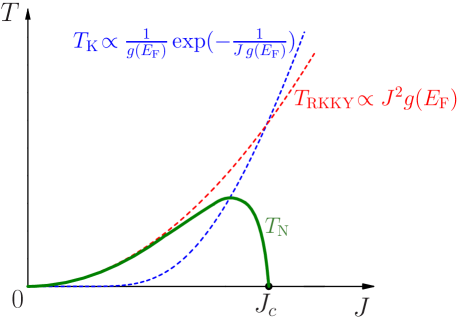
Figure 5: Phase diagram of heavy fermion metals as inspired by Doniach [89]. Here, $J$ refers to the Kondo exchange coupling between the spins of the $f$ and conduction electrons and $g(E_{\rm F})$ to the density of states (DOS) at $E_{\rm F}$.

schematically shown in Fig. 5. At low antiferromagnetic Kondo coupling ($J$) values, the RKKY interaction (characterized by the energy scale $T_{\rm RKKY}\propto J^{2}$) dominates the Kondo screening temperature ($T_{\rm K}\propto e^{-1/J}$) and the system orders magnetically. At high values of $J$, on the other hand, the Kondo screening prevails and the system condenses into a sea of highly interacting quasiparticles with LFL characteristics. The resurgence in the field of heavy fermions is predominantly due to current interest in quantum critical behavior. This behavior is observed if the material undergoes a continuous phase transition at absolute zero temperature; in the scenario just discussed such a transition can take place from a magnetically ordered phase into a heavy LFL one, with the latter representing an ordered state in $\boldsymbol{k}$-space. Within the framework of Doniach’s description of the Kondo lattice, systems for which such phenomena are likely to occur are those where the Kondo effect and the RKKY interaction have comparable energies, i.e., for intermediate values of $J$. A quantum phase transition can then be brought about by a well-directed change of a non-thermal experimental (“control”) parameter such as chemical doping, pressure or magnetic field [4]. While the former two can directly influence the value of $J$ (e.g. via changed lattice parameters) the latter may suppress antiferromagnetic order and, in particular for transverse field tuning, even ferromagnetic order. Even though such a quantum phase transition at $T=0$ is not directly accessible to experiment it affects the finite temperature properties of the material if investigated sufficiently close to the QCP at which the continuous phase transition takes place in the temperature–control parameter diagram [5]. The Landau Fermi liquid theory of conventional metals breaks down in the vicinity of such instabilities, and anomalous experimental behavior like a power-law temperature dependence of the electrical resistivity ($\varrho(T)-\varrho(T\!=\!0)\propto T^{\epsilon}$ where $1\leq\epsilon<2$) [7], a diverging specific heat coefficient [8] and even an apparent violation of the Wiedemann-Franz law [10] have now been observed in heavy fermion systems.

Experimentally, quantum critical behavior and unconventional superconductivity are often found in close vicinity in phase space in this class of materials. In addition to the compound CeCu₂Si₂ [2], the compounds in which the phenomenon has been observed include other Ce [90, 91], but also U [3, 92, 93, 94, 95] and more recently a Yb [96] based system. The observation of superconductivity in these systems which are comprised of a dense array of magnetic atoms is striking since the conventional BCS theory predicts that the presence of even very small amounts of magnetic impurities is highly detrimental to the formation of the superconducting condensate. The fact that superconductivity can exist in an inherently magnetic environment has forced researchers to think beyond the conventional scenario of phonon-mediated superconductivity. The driving force for Cooper pair formation in these heavy fermion metals is believed to be electronic (or more specifically, magnetic) in origin [97, 98, 99, 100, 6]. In case of the compound CeCu₂Si₂, an inelastic neutron scattering study of the magnetic excitation spectrum provided indications for superconducting pairing resulting from antiferromagnetic excitations in this prototypical heavy-fermion compound [101]. An earlier dramatic manifestation of this aspect is the superconductivity observed when a continuous magnetic phase transition is suppressed to absolute zero temperatures, in other words in the vicinity of a QCP [11]. This has also reinforced the connection of heavy fermion systems with the high transition temperature superconducting cuprates. For the latter, one of the competing scenarios is that a QCP lies beneath the superconducting dome and is responsible for both superconductivity as well as the strange metallic (non-Fermi-liquid like) behavior observed in an appreciable region of the experimentally accessible phase space [102].

The formation of the heavy fermion state and superconductivity in these materials has been a subject of extensive investigations in recent years, the details of which are beyond the scope of this article. We refer the reader to some comprehensive reviews devoted to both the experimental and theoretical aspects of these systems [1, 103, 104, 5, 105].

2.6 Anomalous Hall effect in heavy-fermion systems

Though the skew scattering mechanism has been used extensively in trying to account for the observed Hall effect in heavy-fermion systems, a few caveats need to be borne in mind. Firstly, the skew scattering mechanism was proposed for systems with ferromagnetic order, i.e., where the time reversal symmetry is irrevocably broken. This criterion is not strictly met in the heavy-fermion systems, although a lack of time reversal symmetry can be induced by the application of a magnetic field. Secondly, these scattering theories considered the simple case in which the same type of electrons are responsible for both magnetism and electrical conduction. In the heavy-fermion systems it is clear that the magnetism arises from localized (partially screened) $f$ electrons, and are thus of a different origin from the conduction $s,p$ or $d$ electrons. A more relevant model here is that by Kondo [106], who considered a situation in which $d$ electrons were localized in a sea of conduction ($s$ shell) electrons. These localized spins can be disordered by the influence of thermal fluctuations and, in turn, can then act as scattering potentials. Thus, the non-periodicity originates in this case from thermal fluctuations of the local spins, and not primarily from the introduction of impurities. Though this $s\!-\!d$ spin-spin interaction itself did not give rise to skew scattering, including the spin-orbit interaction of the $d$ electrons within the magnetic ions did result in skew scattering, and thus an anomalous contribution to the Hall effect. A related treatment of the Kondo model was presented by Maranzana [107] who considered a ($d$-spin–$s$-orbit) interaction which described the force acting on moving electrons as a consequence of the magnetic field produced by the magnetic $d$ ions. This was used to reproduce the temperature dependence of the anomalous Hall effect in some ferromagnets as well as the abrupt decrease in the Hall coefficient at the antiferromagnetic transition temperature ($T_{N}$), though the calculated values were smaller than the experimentally measured ones. A similar model was also applied by Giovannini to explain the experimentally observed anomalous Hall effect in some dilute magnetic alloys [108].

Considerable theoretical insight into the Hall effect in the heavy-fermion systems originates from the early work by Fert [109] who considered the skew scattering in alloys containing Ce impurities. Using a Coqblin-Schrieffer interaction [110], which considers a 4$f^{1}$ configuration of Ce and its interaction with the conduction ($s$) electrons, a reasonable agreement with the low-field experimental data of some La-Ce alloys was established. Subsequently, a model pertaining to a Kondo lattice system was used [111, 112] in an effort to explain the early experimental signatures observed in the heavy-fermion metals. Here, the ground state was modeled by a degenerate effective $f$ resonance level with an unquenched orbital moment. Application of a magnetic field lifts the degeneracy of the resonance level due to Zeeman splitting, and gives rise to skew scattering of the band electrons. It is to be noted that both these models were effectively meant to be applied to the incoherent Kondo regime ($T\gg T_{K}$) where the Kondo ions scatter independent of each other; they were not strictly valid for the low temperature regime ($T\ll T_{K}$), where a coherent heavy-fermion band condenses out of the local moment landscape. Nevertheless, their results could—at least qualitatively—be extended down to the coherent regime. Combining both these approaches, a generic interpretation of the Hall effect in the heavy-fermion systems was put forward [16] which is schematically shown in Fig. 6. It was concluded that

Figure 6: Modeling of the Hall effect in heavy-fermion compounds. Reprinted figure with permission from A. Fert and P.M. Levy, Physical Review B 36, 1907 (1987) [16]. Copyright © (1987) by the American Physical Society.

the skew scattering contribution increases as the temperature is lowered and attains a maximum at the temperature $T_{\rm coh}$ where spatial coherence sets in. At even lower temperatures this contribution rapidly falls down to zero. In the high temperature regime, the Hall effect arising due to skew scattering is proportional to the product of the magnetic susceptibility ($\chi$) and the magnetic contribution to the resistivity ($\varrho_{M}$). Well below $T_{\rm coh}$, the Hall effect is primarily composed of the ordinary Hall effect, in addition to a small contribution from defects or impurities. This inference is striking, for it suggests that at very low temperatures the measured Hall effect is an intrinsic quantity and thus can be effectively used to monitor the evolution of the Fermi surface. This has now been exploited in the investigation of quantum critical phenomena, an aspect which will be dealt in detail in section 5.

Since the anomalous Hall effect exhibits the just described maximum at the onset of the Kondo coherence, it is not surprising that a large positive maximum followed by a precipitous drop was observed in the measured Hall signal of a number of Ce and U based heavy-fermion systems [113, 114, 115, 116, 117, 118, 119]. In these reports, this drop in the measured Hall response was usually ascribed to the formation of a coherent band which drastically reduces electron scattering. In some systems, such as CePd₃, CeBe₁₃ and CeCu₆, the drop in the Hall coefficient was accompanied by a change of its sign. This change of sign of $R_{\text{H}}$ was accounted for by the models described above in spite of their limited validity in the low temperature ($T\ll T_{K}$) regime. For instance, Ramakrishnan and coworkers had predicted [112] that the Hall coefficient can be written as

$$R_{\rm H}=R_{0}+g\mu_{B}|\alpha|\,\varrho\sin(\phi+\delta_{2})/\sin\delta_{2}\;.$$ (6)

Here $g$ is the gyromagnetic ratio of the $f$ electrons, $\mu_{B}$ is the Bohr magneton and $\delta_{2}$ refers to the phase shift due to scattering in the $l=2$ channel. In addition, $\alpha$ is proportional to $\chi_{1}(1-\chi_{1}T)$ where $\chi_{1}$ refers to the reduced susceptibility. If the resonant scattering in the $l=3$ channel at low temperatures gives rise to a phase shift $\delta_{3}$, then $\phi$ changes from $-\pi$ to $-2\delta_{3}$ as one traverses from the high temperature ($T\gg T_{K}$) regime to the low temperature ($T\ll T_{K}$) one. According to this model, in the high temperature regime, $\phi=-\pi$, and thus the anomalous Hall contribution is always positive. In the low temperature regime one finds $\phi=-2\delta_{3}$ and—interestingly—here the Hall effect can have either sign. However, based on measurements on the Ce_1-xY_xPd₃ alloys, it was suggested that this change of sign in $R_{H}$ is solely associated with the onset of coherence [120]. This was demonstrated by the fact that in compounds with finite Y substitution, in which no low-temperature coherent state is attained, the Hall coefficient $R_{\text{H}}$ decreased monotonically as a function of decreasing temperature. Qualitatively similar behavior was also observed in the system Ce(Pd_1-xAg_x)₃ [113]. These results are in contrast to those observed for the undoped compound CePd₃, where the formation of a low-temperature coherent state is accompanied by a sign change in $R_{\text{H}}$. The experimental signature of the onset of coherence appeared to be much sharper in the Hall effect if compared to that typically seen in resistivity measurements [121]. This difference is exemplary demonstrated for the system CeCu₆ in Fig. 7.

In many heavy-fermion systems, the onset of the low-temperature coherent state is interrupted by the emergence of long-range (antiferro-)magnetic order. In the system U₂Zn₁₇, it was shown that $R_{H}$ increases abruptly at the onset of the antiferromagnetic order [122]. It was suggested that this change reflects the opening of a gap at the Fermi surface due to magnetic ordering. In the system CePtSi, this increase was seen to be more dramatic, with the Hall constant increasing by a factor of 15 on entering the antiferromagnetically ordered regime [119]. Moreover, below the Néel transition temperature $T_{N}$, the Hall resistivity was highly nonlinear, and also exhibited signatures of a possible metamagnetic transition. However, the resistivity was almost constant around $T_{N}$, thus prompting the authors to conclude that the observed features

Figure 7: Comparison of the resistivity $\varrho$ ($\circ$ and right scale) and the Hall coefficient $R_{\text{H}}$ ($\scriptstyle\blacksquare$ and left scale) at the onset of the coherent state in CeCu₆. Reprinted figure with permission from T. Penney et al., Physical Review B 34, 5959(R) (1986) [121]. Copyright © (1986) by the American Physical Society.

cannot be accounted for on the basis of a Fermi surface modification alone, which would have affected the resistivity and Hall measurements in similar fashions. Thus, irrespective of the interpretation of the observed Hall coefficient across the antiferromagnetic transition, the sensitivity of this measurement in tracking such transitions is beyond doubt. Moreover, it appears to be larger than that commonly observed in resistivity measurements. This has been reinforced by measurements on the heavy-fermion system URu₂Si₂ where a transition at 17.5 K has been the focus of extensive investigations. The challenge here is to reconcile the large entropy release and the accompanying gap in the magnetic excitation spectrum with the anomalously small value ($\sim 0.03\;\mu_{B}/U$) of the magnetic moment, giving rise to suggestions that a “hidden order” coexists and probably competes with the antiferromagnetic order in this system [123]. Early investigations in URu₂Si₂ revealed that the Hall coefficient $R_{\text{H}}$ exhibits a sharp anomaly at this transition [124]. An analysis based on the model by Fert and Levy [16] has been used to extract a carrier density of about 0.04 holes/U above the transition, but is an order of magnitude smaller below the transition [125]. In combination with Nernst effect measurements, it was thus inferred that this transition is accompanied by a reconstruction of the Fermi surface into small high-mobility pockets, resulting in an abrupt increase in the entropy per itinerant charge carrier and a decrease of the scattering rate [126]. Recently, Hall effect measurements have been extended up to magnetic fields of the order of 45 T and revealed a cascade of field induced transitions accompanied by changes in the Fermi surface topology [127, 128].

3 Theoretical Work on the Hall effect

3.1 Theoretical Overview

While the conceptual basis of the Hall effect is accessible enough for it to be captured in a simple sentence—a manifestation of the perpendicular Lorentz force on moving charges—the interpretation of Hall measurements can be considerably more challenging. Spectroscopies are usually the more straightforward experimental quantities to connect to the underlying theory because they often directly measure a response function. In transport theory it is the elements of the appropriate conductivity tensor that are related to correlation functions [129]—current-current for the electrical conductivity. However the Hall resistivity (which is the quantity typically measured in experiment) is not related to a single correlation. Rather it is a ratio of conductivities through the inverse of the conductivity tensor. One is helped to some extent by the Onsager relation for the off diagonal elements of the conductivity (e.g. $\sigma_{xy}=-\sigma_{yx}$). Nevertheless the measured quantities can look complex:

$$\rho_{xy}=-\frac{\sigma_{xz}\sigma_{yz}-\sigma_{xy}\sigma_{zz}}{\sigma_{xz}^{2}\sigma_{yy}+\sigma_{yz}^{2}\sigma_{xx}+\sigma_{xy}^{2}\sigma_{zz}+\sigma_{xx}\sigma_{yy}\sigma_{zz}}\xrightarrow[\rm symmetry]{\rm tetragonal}-\frac{\sigma_{xy}}{\sigma_{xy}^{2}+\sigma_{xx}^{2}}\;.$$ (7)

Fortunately for materials with high symmetry and in the weak field limit, this ratio can lead to cancellations between numerator and denominator. This can, in turn, give direct insight into physically measurable quantities, of which carrier concentration in doped semiconductors is one elementary example. It is remarkable that the heavy fermion systems may equally allow quite simple interpretations of the Hall effect as we will show later.

Although the Hall resistivity may not be directly related to a response function, it has been shown that the related quantity—the tangent of the Hall angle $\theta_{\rm H}$ as defined by eq. (3)—is [130]. Physically $\theta_{H}$ is the angle of deflection a free current would experience in a transverse magnetic field. Its role as a response function means that the frequency dependent Hall angle can be integrated to provide a sum rule independent of the underlying microscopic physics [130]. Optical Hall angle measurements have been undertaken in the cuprates [131], but not yet in the heavy fermion metals.

3.2 Key results from Boltzmann theory

The most elementary theoretical treatment of the Hall effect is via a semi-classical Boltzmann equation in the relaxation time approximation which is well described in standard texts [132]. It assumes fermionic excitations with a Fermi surface determined by a given dispersion relation and that the collision processes can be approximated by a decay time to equilibrium. In section 3.4 we consider the limitations of this approach. Nevertheless, this is likely to be valid in the low temperature limit of the Fermi liquid state when impurity scattering dominates. The simple results of such an approach already illustrate a number of important features of magnetotransport in general.

Within the Jones-Zener expansion the conductivities are found order by order in magnetic field [133], and are related to surface integrals around the Fermi surface. The conductivities are defined by

$$j_{\alpha}=\sigma_{\alpha\beta}E_{\beta}+\sigma^{(1)}_{\alpha\beta\gamma}E_{\beta}B_{\gamma}+\sigma^{(2)}_{\alpha\beta\gamma\delta}E_{\beta}B_{\gamma}B_{\delta}+\cdots\;,$$ (8)

where

$$\sigma_{\alpha\beta} = \int e^{2}\tau\frac{\partial f^{0}}{\partial\varepsilon}v_{\alpha}v_{\beta}\;d^{3}k\;,$$ (9)

$$\sigma^{(1)}_{\alpha\beta\gamma} = \epsilon_{\gamma\delta\sigma}\int e^{3}\tau^{2}\frac{\partial f^{0}}{\partial\varepsilon}v_{\alpha}v_{\sigma}M^{-1}_{\beta\delta}\;d^{3}k\;,$$ (10)

$$\sigma^{(2)}_{\alpha\beta\gamma\delta} = \epsilon_{\rho\gamma\nu}\epsilon_{\mu\delta\sigma}\int e^{4}\tau^{3}\frac{\partial f^{0}}{\partial\varepsilon}v_{\alpha}v_{\rho}\left\{M^{-1}_{\sigma\beta}M^{-1}_{\mu\nu}+\frac{v_{\mu}}{\hbar}\frac{\partial}{\partial k_{\beta}}\left(M^{-1}_{\sigma\nu}\right)\right\}d^{3}k\;,$$ (11)

$\epsilon_{\alpha\beta\delta}$ is the antisymmetric tensor, and the inverse effective mass is

$$M^{-1}_{\alpha\beta}=\frac{1}{\hbar^{2}}\frac{\partial^{2}\varepsilon}{\partial k_{\alpha}\partial k_{\beta}}\;.$$ (12)

As can be seen, each conductivity is an integral over the Fermi surface (since the energy derivative of the Fermi function, $f^{0}$, is approximately a delta function). Furthermore, higher order dependence on the external magnetic field is related to a higher order derivative of the dispersion ($\varepsilon_{k}$) around the Fermi surface. This suggests that magnetotransport is, with each increasing order of field, a sensitive probe of the details of the Fermi surface.

These expressions reduce to the “pre-quantum” forms of Drude for the case of a parabolic dispersion ($\sigma_{xx}=ne^{2}\tau/m$, $\sigma_{xy}=\omega_{c}\tau\sigma_{xx}$) so that the Hall coefficient $R_{H}=\rho_{xy}/B=1/ne$. However, they now account for the otherwise mysterious observation that the Hall effect can change sign. This was first recognized by Peierls who showed how the almost full band of electrons produces the same Hall effect as an almost empty band of positively charged carriers because of the sign of the curvature of the Fermi surface. In the case of a multiband system then conductivities arising from each band must be added together before the resultant conducivity tensor is inverted. This of course spoils the simple relationship between carrier density and Hall constant even for a parabolic band. A peculiar case of note emerges for compensated metals (where the Hall conductivity of the individual bands in, say, a two band system are equal and opposite and so cancel). Under these circumstances the leading contribution to the measured Hall effect occurs at higher order so $\rho_{xy}\sim B^{2}$ [80, 81]. The latter has been demonstrated to hold by high-field experiments on the heavy fermion metal UPt₃ [82]. This aspect will be important for the discussion of the Hall effect on Ce$M$In₅ systems, sections 6.3.2 and 6.3.3.

Some rather beautiful results have been proved by Ong within Boltzmann transport theory in the 2D limit which give geometric interpretation to magnetotransport quantities [25]. The Hall conductivity can be related to the flux through the area swept out by the mean free path as it traced around the Fermi surface. The magnetoresistance is related to the variance of the local Hall angle around the Fermi surface [134].

The Boltzmann equation can also be solved in the limit of high magnetic field as an expansion in $1/B$ (though of course Landau level quantization means that this limit is never strictly obtained). Under these conditions the Hall effect becomes insensitive to Fermi surface shape and can be directly related to the volume of the Fermi surface. In this limit even in a multiband system one can use the Hall effect to determine the carrier concentration independent of band structure details $R_{H}=1/e(\sum_{i}n_{i})$. It is arguable as to whether this limit is ever physically relevant.

Finally, while the results quoted above relate to solutions obtained via expansion in magnetic field (either low field or high field), it is not necessary to solve the Boltzmann equation by expansion. The conductivity can be obtained to all orders in the field at the expense of an additional surface integral using the so-called Chambers formula [135]. Such an approach is necessary when dealing with quantities which vary rapidly around the Fermi surface as the Jones-Zener expansion can breakdown. This will be important at a density wave transition for example (see later).

These results from Boltzmann theory are often very useful as a starting point to understand magnetotransport phenomena in the heavy fermion metals. In fact, sometimes they are all one can do. However, to make further progress we proceed to consider the foundations of this approach within Fermi liquid theory and thence the physics beyond.

3.3 Hall effect within Fermi liquid theory

A more formal justification for the Boltzmann approach (and thereby revealing its limitations) is obtained through the Kubo formula and its diagrammatic representation. Direct methods of calculating typically involve treating the magnetic field perturbatively. Given we are looking for the current response to an electric and magnetic field in the lowest order, the Hall conductance involves a three current correlation. This issue of maintaining gauge invariance in these calculations requires that Ward identities be preserved [136]. In essence this means that the treatment of vertex corrections must be consistent with the self-energy (i.e. that every process included in the self-energy has a corresponding vertex correction obtained by including a current vertex at any point within the self-energy diagram).

The simplest question concerns the recovery of the results of Boltzmann theory in the relaxation time approximation. If one assumes non-interacting electrons and dilute impurities then these relaxation time approximation results above can be obtained if one assumes $s$-wave potential scattering [137]. The isotropic scattering ensures that the calculation is insensitive to vertex corrections. It also suggests that in the case of strongly momentum dependent scattering which might be expected near a QCP then reliance on the relaxation time approximation may be suspect.

Treating the problem of interacting fermions is considerably more difficult. However, a remarkable simplification ensues if one is limited to systems where the low energy physics can be described within Fermi liquid theory [83]. In Landau Fermi liquid theory the low lying excitations of the interacting system are adiabatically connected to a non-interacting Fermi gas (a pedagogical account being found in Refs. [138, 139]). Landau considered a neutral Fermi liquid in deriving the transport equation, but the extension of this equation to the charged case is straightforward and dictated by minimal coupling. The derivation assumes that the Fermi liquid is characterized by a coarse-grained distribution of quasiparticles $n(\bm{p},\bm{r},t)$ (i.e. the $\bm{r}$ dependence is slowly varying on the length scale of the Fermi wavelength). Under these conditions the local quasiparticle energy can be considered to be the effective classical Hamiltonian of the quasiparticle

$$\epsilon(\bm{p},\bm{r})=\epsilon^{0}(\bm{p})+\sum_{\bm{p}^{\prime}}f_{\bm{p}\bm{p}^{\prime}}\delta n(\bm{p}^{\prime},\bm{r})\;,$$ (13)

where the interaction is assumed to be local on the scale of spatial coarse graining. Minimal coupling introduces the electric and magnetic fields through the vector potential $\bm{p}\rightarrow\bm{p}-e\bm{A}$. The time evolution of the distribution is then determined by the total time derivative

$$\frac{dn}{dt}=\frac{\partial n}{\partial t}+{\bm{\nabla}}_{\bm{r}}n\cdot\frac{\partial\bm{r}}{\partial t}+{\bm{\nabla}}_{\bm{p}}n\cdot\frac{\partial\bm{p}}{\partial t}=I\;,$$ (14)

where $I$ is the collision integral. Using Hamilton’s equation of motion and expressing the result in terms of the deviation from local equilibrium, $\delta n(\bm{p},\bm{r})=n(\bm{p},\bm{r})-n_{0}(\epsilon_{\bm{p}}(\bm{r}))$, we find for steady state, translationally invariant solutions

$$e\bm{E}\cdot\bm{\nabla}_{\bm{p}}n_{0}+e\bm{v}\times\bm{B}\cdot\bm{\nabla}_{\bm{p}}\delta n=I\;.$$ (15)

This is exactly the result one would write down for simple Boltzmann transport yet it includes the electron-electron interaction within the Fermi liquid formalism.

Establishing that this result is rigorous within a diagrammatic approach was achieved by Betbeder-Matibet and Nozières [140] and by Khodas and Finkel’stein [141]. Thus the quasiparticle renormalization, $Z$, and other interaction corrections all cancel in the Hall coefficient at least to zeroth order in $1/\tau E_{F}$. Thus we conclude that if a Fermi liquid state emerges at low temperatures in the heavy fermion system, then transport can be described within a Boltzmann-like formalism.

3.4 Quantum critical heavy fermion metals

All the results of the previous discussion require the existence of Fermi liquid like quasiparticles. Understanding the Hall effect without quasiparticles is more challenging [142]. Here we focus on what can be learnt from the Hall coefficient and higher order magnetotransport coefficients in the heavy fermion systems and will argue that the most useful diagnosis is obtained in the $T\rightarrow 0$ limit where a Fermi liquid like picture should emerge. The heavy fermion metals hold particular interest here since their inherently small energy scales mean that relatively weak perturbations like pressure or magnetic field are able to tune magnetic transition temperatures to absolute zero.

At zero temperature the QCP can be viewed a transition between Fermi liquids but the nature of that transition is a matter of very active interest. Two scenarios are emerging. On the one-hand, the nature of the QCP could be dictated by the fluctuations associated with a magnetic transition driven or tuned to zero temperature. This QCP might refer to as a conventional one—though as we will show the theoretical description remains challenging in a number of physically relevant cases. In this case the Fermi liquids on either side of the quantum critical point would be both adiabatically connected to the same non-interacting Fermi gas (albeit evolving continuously as the density wave gap opens at the transition point).

An alternative view is that the essence of the QCP in heavy fermion metals is associated with the zero temperature breakdown of the Kondo effect. In that scenario the magnetic instability plays a secondary role as a mechanism to quench the spin entropy of the local moments. In this scenario while the QCP would divide the zero temperature axis into two Fermi liquids, these two states would be adiabatically connected to entirely different non-interacting systems. A central tenant of this review is that the low temperature Hall data can play a key diagnostic role in discriminating between these two scenarios.

3.4.1 “Conventional” Hertz-Moriya-Millis quantum criticality

We begin by considering the Hall effect at a “conventional” SDW QCP. The effective action for quantum criticality in a metal has been argued to be the so called Hertz-Moriya-Millis action [4, 30, 31]

$$S=\frac{1}{\beta}\!\int\!d^{D}q\sum_{n}\phi_{-q,-\omega_{n}}E_{0}\!\left[r_{0}+\xi_{0}^{2}q^{2}+\frac{|\omega_{n}|}{\Gamma_{q}}\right]\phi_{q,\omega_{n}}+u\!\int\!\!d^{D}{\boldsymbol{r}}\int_{0}^{\beta}\!\!d\tau|\phi({\boldsymbol{r}},\tau)|^{4}+\cdots\;.$$ (16)

In its simplest terms this action can be viewed as the quantum extension of the Ginsburg-Landau free energy functional in the vicinity of a continuous phase transition where the form of the expansion is deduced by symmetry and analyticity. The frequency sum of bosonic Matsubara frequencies is a consequence of the quantum nature of the transition (i.e. that the order parameter is not an eigenstate of the Hamiltonian and so must be summed over in imaginary time). This action can be obtained from a random phase approximation (RPA)-like saddle-point treatment of the interacting fermion problem [4]. The non-analytic term in $\omega_{n}$ arises from the damping induced by the electron fluid on the order parameter. The form of the damping rate depends on the conservation laws applied to the order parameter:

$$\Gamma_{q}\sim q^{z-2}=\left\{\begin{array}[]{ll}\Gamma_{0}&\quad(z=2)\quad\text{antiferromagnetic},\\ v_{F}q&\quad(z=3)\quad\text{clean ferromagnet},\\ Dq^{2}&\quad(z=4)\quad\text{dirty ferromagnet}\>.\\ \end{array}\right.$$ (17)

The experimental consequences of this action have been well studied and so too have been the conditions for its validity. These issues have been reviewed [5] but in brief the low energy particle-hole excitations of the metallic state cannot generally be safely integrated out to yield the action above [143]. The problem is particularly acute for clean ferromagnetic instabilities where the soft particle-hole excitations generate non-local terms in the effective action for the order parameter and would seem to generically drive the transition first order [144]. The case of two dimensional antiferromagnets is also problematic from a theoretical standpoint [145].

Because of the theoretical questions concerning the precise nature of the magnetic QCP in itinerant systems, for the purpose of this review we consider only the antiferromagnetic case and that at two levels. The first is the finite temperature effect of antiferromagnetic spin fluctuations on transport and the Hall effect. The second is the zero temperature limit.

3.4.2 Spin-fluctuation theory

At a phenomenological level one can introduce a form of the spin-fluctuations first introduced in the context of the high temperature cuprate materials [146]:

$$\chi^{s}_{\bm{q}}(\omega)=\sum_{\bm{Q}}\frac{\chi_{\bm{Q}}}{1+\xi^{2}(\bm{q}-\bm{Q})^{2}-i\omega/\omega_{\rm sf}}\;.$$ (18)

Here $\omega_{\rm sf}$ and $\chi_{\bm{Q}}$ scale with the square of the magnetic correlation length, $\xi^{2}$, and $\bm{Q}$ are the Fourier modes of the incipient magnetic order. Transport is then dictated by quasiparticle scattering from spin fluctuations. Two effects control the resulting transport which can be considered within Boltzmann transport.

Firstly, the strong momentum dependence of the fluctuations strongly scatters particles on the Fermi surface connected by the ordering wave vectors ${\bm{Q}}$, while leaving other parts of the Fermi surface relatively unscathed. The Fermi surface divides into ”hot-spots” where scattering is strong and “cold regions” where it is not [147]. One issue within this scenario is the observation that the cold parts should short-circuit the transport and so render the metal relatively insensitive to the presence of the magnetic fluctuations [148]. Within such a picture a relaxation time approximation has been invoked [149]. This produced a number of criticisms of the spin-fluctuation model as it applied to the cuprates. The origin of these criticisms is the observation made previously that magnetotransport is very sensitive to anisotropy around the Fermi surface and so a hot-spot–cold-region model generates a large magnetoresistance [134, 150] (much larger than that seen in the cuprates).

The second effect is that the fluctuation performing the scattering is itself a particle-hole excitation of the fluid and this modifies the current. This has been emphasized by Kontani who recognized this effect within a tour-de-force diagrammatic approach to high order transport coefficients in a magnetic field (for a recent review see Ref. [29]). In diagramatics this appears as a current vertex correction but its effect can be modelled within Boltzmann transport provided one does not make the relaxation time approximation but considers the collision integral in detail.

Taking both of these effects together, Kontani’s analysis of the spin fluctuation model claims that one can obtain a strongly temperature dependent Hall coefficient in the presence of antiferromagnetic fluctuations: $R_{\rm H}\sim\xi^{2}\sim 1/T$. Moreover, higher order terms in magnetotransport do not get anomalously large as they would in the relaxation time approximation but adopt a temperature dependence associated with the Hall effect. One consequence is that the magnetoresistance $\Delta\rho/\rho_{0}$, which in the relaxation time approximation would be expected to scale like $\rho_{0}^{-2}$ (Kohler’s rule, Ref. [151]), does not. Rather it would behave like $\xi^{4}/\rho_{0}^{2}\sim T^{-4}$ leading to a modified Kohler’s rule $\Delta\rho/\rho_{0}\sim(R_{\rm H}/\rho_{0})^{2}$.

The observations above are, at face value, very reminiscent of the behaviour of the normal state of the high temperature cuprates superconductors. There, Anderson [27] and Ong [24] noticed that $\cot\theta_{H}$—which should, within the relaxation time approximation, be proportional to the scattering rate as measured in the resistivity (i.e. $\sim T$)—here behaved with a distinct $T^{2}$ temperature dependence (cf. Fig. 28 and related discussion in section 7.1.1; see also the discussion on results obtained on Ce$M$In₅ materials, section 6.3.4). Crucial to their observation was the disorder dependence on the introduction of Zn impurities into the cuprates. They identified $\rho$ and $\cot\theta_{H}$ as measuring entirely separate scattering rates because while both had very different temperature dependencies, they both also showed Matthiesen’s rule type behavior as a function of impurity concentration: Impurity scattering behaved additively to both the scattering rates. In the context of the cuprates this is a strong constraint on the underlying mechanism for the temperature dependence of the Hall coefficient.

Adding disorder to a quantum critical antiferromagnetic metal was considered by Rosch [152]. He showed that there is a strong interplay between even very small amounts of disorder and antiferromagnetic fluctuations. The disorder smears out the hot-spots on the Fermi surface thereby considerably weakening the short-circuiting argument of Hlubina and Rice. Moreover, the expected temperature dependencies of the resistivity are also modified from those of the spin-fluctuation model. Rosch also showed that very small amounts of disorder are sufficient to render the Hall coefficient relatively weakly dependent on temperature [153]. This is somewhat at odds with the Kontani calculation which claims that the $\cot\theta_{H}$ behavior remains distinct from the resistivity albeit with a weaker than $T^{2}$ power law.

Given that there remains some uncertainty about the precise temperature/disorder dependence of the Hall coefficient when it is dominated by quantum critical fluctuations, we argue that the $T=0$ limit provides a more reliable domain for the Hall effect’s interpretation. At temperatures low enough that the inelastic scattering is a relatively small fraction of the overall resistivity, one is dominated by elastic impurity scattering. Under these circumstances a relaxation time approximation is valid and one can use the magneto-transport data to characterize changes in the Fermi surface.

Initial studies suggested that at a continuous density wave transition all transport quantities should vary smoothly [28, 48]. However, these considerations were based on a weak field expansion. Crucially near a QCP there is an order of limits question as to whether the field scale goes to zero before the density wave gap [50, 52]. A weak field expansion is valid only if

$$B\tau<\frac{\Delta}{ev_{F}^{2}}\;,$$ (19)

where $\tau$ is the relaxation time and $\Delta$ the density wave gap. Near enough to the QCP this expansion will breakdown for any finite field experiment in the ordered phase. The consequences are the Hall effect and resistivity develop non-analytic terms in field $\omega_{c}\tau$. These arise whenever the Fermi surface crosses the density wave Brillouin zone so Bragg reflection causes the Fermi surface to develop a sharp corner. Under these circumstances the Hall conductivity develops an additional term that goes like $|\omega_{c}\tau|^{2}$ and the longitudinal conductivity a term that behaves like $|\omega_{c}\tau|$. These terms are absent in the paramagnetic phase so this implies that there is a discontinuity in the Hall effect and in the resistivity of order $|\omega_{c}\tau|^{2}$ and $|\omega_{c}\tau|$ respectively at the transition point. These discontinuities are rounded by magnetic breakdown effects and are suppressed by disorder. Nevertheless, the observation of a magnetoresistance linear in magnetic field is often indicative of a sharp feature (point of small radius of curvature) on the Fermi surface.

In summary, the theory of the Hall effect in a conventional density wave type QCP is least ambiguous in the zero temperature limit. Here we expect to see rather smooth evolution of the weak field Hall constant through the transition (unless the system is unusually clean when it may be possible to see discontinuities due to the reconstruction of the Fermi surface). At finite temperature, Kontani predicts that antiferromagnetic fluctuations can give rise to a temperature-dependent Hall coefficient though Rosch argues that this temperature dependence is lost with relatively small quantities of disorder.

3.5 Hall effect across Kondo breakdown quantum critical point

3.5.1 Quantum criticality in heavy fermion metals and jump of Hall coefficient

Theoretical studies of quantum phase transitions in heavy fermion metals depart from the Kondo lattice Hamiltonian:

$${\cal H}=\frac{1}{2}\sum_{ij}I_{ij}~{}{\bf S}_{i}\cdot{\bf S}_{j}~{}+~{}\sum_{\bf k\sigma}\epsilon_{\bf k}c_{{\bf k}\sigma}^{\dagger}c_{{\bf k}\sigma}+~{}\sum_{i}J_{K}~{}{\bf S}_{i}\cdot{\bf s}_{c,i}\;.$$ (20)

Here, a lattice of spin-$1/2$ local moments interact with each other with an exchange interaction $I_{ij}$. To specify the typical strength of the exchange interaction, we use $I$ to label the nearest-neighbor interaction, and we will focus on the case that it is antiferromagnetic. The model also contains a conduction-electron band, $c_{{\bf k}\sigma}$, with a band dispersion $\epsilon_{\bf k}$ and bandwidth $W$. At each site $i$, the spin of the conduction electrons, ${\bf s}_{i,c}=(1/2)c_{i}^{\dagger}{\boldsymbol{\tau}}c_{i}$, where ${\boldsymbol{\tau}}$ are the Pauli matrices, is coupled to a spin-$1/2$ local moment, $\bf{S}_{i}$, via an antiferromagnetic Kondo exchange interaction $J_{K}$.

When the Kondo coupling dominates over the RKKY interaction, the ground state is a Kondo singlet (cf. section 2.5). The Kondo screening effect leads to Kondo resonances, which are charge-$e$ and spin-$1/2$ excitations. There is one such Kondo resonance per site, and these excitations induce a “large” Fermi surface [154, 155, 156, 157, 158]. Consider that the conduction electron band is filled with $x$ electrons per site; for concreteness, we take $0<x<1$. The conduction electron band and the Kondo resonances will be hybridized, resulting in a count of $1+x$ electron per site. The Fermi surface would therefore have to expand to a size that encloses all these $1+x$ electrons. This defines the large Fermi surface.

Consider the conduction electron Green’s function:

$$G_{c}({\bf k},\omega)\equiv F.T.[-<T_{\tau}c_{{\bf k},\sigma}(\tau)c_{{\bf k},\sigma}^{\dagger}(0)>]\;,$$ (21)

where the Fourier-transform ($F.T.$) is taken with respect to $\tau$. This Green’s function is related to a self-energy, $\Sigma({\bf k},\omega)$, via the standard Dyson equation:

$$G_{c}({\bf k},\omega)=\frac{1}{\omega-\epsilon_{\bf k}-\Sigma({\bf k},\omega)}\;.$$ (22)

In the heavy Fermi liquid state, $\Sigma({\bf k},\omega)$ is non-analytic and contains a pole in the energy space [154, 156, 157]:

$$\Sigma({\bf k},\omega)=\frac{(b^{*})^{2}}{\omega-\epsilon_{f}^{*}}\;.$$ (23)

Inserting eq. (23) into eq. (22), we end up with two poles in the Green’s function:

$$G_{c}({\bf k},\omega)=\frac{u_{\bf k}^{2}}{\omega-E_{1,{\bf k}}}+\frac{v_{\bf k}^{2}}{\omega-E_{2,{\bf k}}}\;.$$ (24)

Here,

$$E_{1,{\bf k}} = (1/2)\left[\epsilon_{\bf k}+\epsilon_{f}^{*}-\sqrt{(\epsilon_{\bf k}-\epsilon_{f}^{*})^{2}+4(b^{*})^{2}}\right]\;,$$

$$E_{2,{\bf k}} = (1/2)\left[\epsilon_{\bf k}+\epsilon_{f}^{*}+\sqrt{(\epsilon_{\bf k}-\epsilon_{f}^{*})^{2}+4(b^{*})^{2}}\;\right]$$ (25)

describe the dispersion of the two heavy-fermion bands. These bands must accommodate $1+x$ electrons, so the new Fermi energy has to lie in a relatively flat portion of the dispersion, leading to a small Fermi velocity and a large quasiparticle mass $m^{*}$.

The self-energy contains only two parameters, the pole strength (i.e., the residue), $(b^{*})^{2}$, and the pole location, $\epsilon_{f}^{*}$. eq. (23) describe only the coherent part with the well-defined pole; an incoherent part will specify damping of the quasiparticle excitations.

In the opposite limit, when the RKKY interaction dominates over the Kondo coupling, the system is antiferromagnetically ordered. For any spatial dimension $d>1$, it follows from a renormalization group study [159] that the Kondo singlet breaks down. Correspondingly, there is no Kondo resonance, and the Fermi surface is “small”, i.e. does not incorporate the $f$-electrons. The conduction-electron self-energy in a large-$N$ limit takes the form

$$\Sigma({\bf k},\omega)=a\omega-i(b|\omega|^{d}+c\omega^{2})\;{\rm sgn}\,\omega$$ (26)

From a comparison with eq. (23), we see that the strength of the pole in the conduction-electron self-energy has vanished. Inserting eq. (26) into eq. (22) gives rise to a Fermi surface that is entirely specified by the conduction electron dispersion.

Quantum phase transition in the Kondo lattice arises by tuning the parameter $\delta\equiv T_{K}^{0}/I$, where $T_{K}^{0}\approx\rho_{0}^{-1}\exp(-1/\rho_{0}J_{K})$ with $\rho_{0}$ being the density of states of the conduction electrons at the Fermi energy [89, 160] (cf. also Fig. 5). In recent years, several theoretical approaches have been undertaken to study the quantum phase transition. The extended dynamical mean field theory (EDMFT) [161, 162] focuses on the destruction of the Kondo effect by the antiferromagnetic fluctuations, leading to two classes of solutions. In one, the Kondo breakdown occurs at the onset of the antiferromagnetic order; this is referred to as local quantum criticality. In another class of solution, the Kondo breakdown takes place inside the antiferromagnetic order. The QCP separating the antiferromagnetic and paramagnetic states has the SDW form, but a Kondo breakdown gives rise to another quantum phase transition inside the antiferromagnetic part of the phase diagram.

The evolution of the Hall coefficient across the local QCP can be most clearly seen in the zero-temperature limit. At $\delta>\delta_{c}$, the ground state is a Fermi liquid, and the conduction-electron self-energy has the form of eq. (23). The associated quasiparticles, with the dispersion given by eq. (25), are located near the large Fermi surface. At $\delta<\delta_{c}$, the ground state is also a Fermi liquid, but now the conduction-electron self-energy, having the form of eq. (26), no longer has the pole and the quasiparticles are located near the small Fermi surface. As discussed earlier in this section, the quasiparticle residue for each Fermi liquid will cancel in its Hall coefficient. Since the underlying non-interacting system for the two Fermi liquids corresponds respectively the fermions with $f$-interactions itinerant or localized, the Hall coefficient has different values in the two Fermi liquids [163]. In other words, the Hall coefficient at zero temperature jumps as the control parameter $\delta$ is tuned through $\delta_{c}$, the QCP.

Another approach to the Kondo breakdown is based on a large-$N$ formulation in conjunction with slave-particle representations of the spin operator. The fermionic representation of the spin provides a means to access a spin liquid when the Kondo amplitude $(b^{*})^{2}$ is suppressed [164, 165], where fermionic spinons and the bosonic $b$ fields are coupled to a gauge field. The Kondo destruction of $b^{*}=0$ corresponds to a metallic state (as opposed to a Bose-Einstein condensate) of the bosonic component. Calculation of the Hall coefficient and longitudinal resistivity in this approach shows a jump of both quantities at the Kondo-breakdown transition at zero temperature [166].

3.5.2 Crossover and scaling of the Hall coefficient at non-zero temperatures

The $T$-$\delta$ phase diagram for the Kondo-destruction local QCP was already illustrated in Fig. 1(b). The energy scale $E_{\text{\small loc}}^{*}$ specifies a corresponding $T^{*}$ line, which separates the phase diagram at low temperatures into two parts. To the right of the $T^{*}$ line, the system flows (in the renormalization-group sense, as energy is lowered) towards a ground state with complete Kondo screening and therefore large Fermi surface; the $T_{\text{\small LFL}}$ scale describes the renormalized Fermi energy for this Fermi liquid state. To the left of the $T^{*}$ line, however, the Kondo screening process is incomplete; in the ground state, the static Kondo screening is absent and the Fermi surface is small. Here, the Néel temperature, $T_{N}$, marks the onset of the antiferromagnetic order. In the zero-temperature limit, the end of the $T^{*}(\delta)$ line, which is at $\delta_{c}$, marks a genuine $f$-electron delocalization-localization phase transition.

Compared to the zero temperature case, the behavior of the Hall coefficient at non-zero temperatures across a Kondo-destruction local QCP is much more difficult to analyze and can only be considered qualitatively. The single-electron Green’s function, $G({\bf k},\omega)$, on either side of the zero-temperature transition can be written as

$$G({\bf k},\omega)=G_{\rm coh}({\bf k},\omega)+G_{\rm inc}({\bf k},\omega)\>.$$ (27)

This decomposition is an immediate consequence of the fact that the phases separated by the QCP are Fermi liquids. The coherent part is given by

$$G_{\rm coh}({\bf k},\omega)=\frac{z_{\bf k}}{\omega-E({\bf k})+i\Gamma_{\bf k}(T)}$$ (28)

describing a quasiparticle, and $G_{\rm inc}({\bf k},\omega)$ is a background contribution. The quasiparticle residue, $z_{\bf k}$, is non-zero in either phase, but $z_{\bf k}$ vanishes as the QCP is approached: $z_{\bf k}\rightarrow 0$ as $\delta\rightarrow\delta_{c}$. At $T=0$, the quasiparticle damping $\Gamma_{\bf k}$ vanishes at the small Fermi-momenta ${\bf k}_{F}^{S}$ for $\delta<\delta_{c}$, and at the large Fermi-momenta ${\bf k}_{F}^{L}$ for $\delta>\delta_{c}$; at these respective Fermi-momenta, the quasiparticles become infinitely-sharp excitations at zero temperature. The coherent part of $G({\bf k},\omega)$ is therefore the diagnostic feature on either side of the transition, and it jumps at the QCP in accordance with the sudden change of the Fermi surface. As already described, this jump is manifested in the Hall measurement (see, e.g., section 5.1 where results obtained on YbRh₂Si₂ are presented), because the Hall coefficient is independent of the quasiparticle residue.

At non-zero temperatures, the quasiparticle relaxation rate at either ${\bf k}_{F}^{S}$ for $\delta<\delta_{c}$, or ${\bf k}_{F}^{L}$ no longer vanishes. In fact, inside the Fermi-liquid phase (with either large or small Fermi surface), the temperature dependence of $\Gamma_{{\bf k}_{F}}$ has to be quadratic in $T$. However, the Fermi surface remains well defined in these regimes. The change from one Fermi surface to the other is restricted to the intermediate quantum critical regime. Because of the absence of a phase transition at any non-zero temperature, the sharp reconstruction of the Fermi surface at $T=0$ is turned into a Fermi-surface crossover across the $T^{*}(\delta)$ line. This implies that the relaxation rate determines the parameter range corresponding the Fermi surface change. From the relation of the Hall coefficient to the Fermi surface we can associate the width of the Hall crossover with this broadening and consequently with the relaxation rate $\Gamma$ of the single-electron Green’s function.

Consider a general scaling form for the single-electron Green’s function at the Fermi momentum in the quantum critical region:

$$G({\bf k}_{F},\omega)=\frac{1}{T^{\alpha}}g\left({\bf k}_{F},\frac{\omega}{T^{x}}\right)\,.$$ (29)

The $\omega/T$ scaling at an interacting fixed point implies $x=1$. The associated relaxation rate, defined in the quantum relaxational regime (${\hbar\omega}\ll k_{B}T$) according to

$$\Gamma({\bf k}_{\mathrm{F}},T)\equiv\left[-i\partial\ln G({\bf k}_{\mathrm{F}},{\omega},T)/\partial{\hbar\omega}\right]_{{\omega}=0}^{-1}\;,$$ (30)

is linear in temperature: $\Gamma({\bf k}_{\mathrm{F}},T)=cT$, where $c$ is a universal constant. Correspondingly, the crossover width is expected to be linear in temperature. This is indeed experimentally observed for YbRh₂Si₂, see Fig. 18 in section 5.1.

4 Experimental aspects of Hall effect measurements in metals

4.1 Measurement techniques

For the following considerations we rely on a discussion of eq. (1) for simplicity. Because of the typically large density of free charge carriers in a metal the Hall coefficient $R_{\text{H}}$ is small. As an example, for aluminum $R_{\text{H}}$ is about $-3.5\cdot 10^{-11}$ m³C^-1 at room temperature [14]. Consequently, even for favorable experimental conditions only a very small Hall voltage is generated. For Al and $I_{x}=100$ mA, $B_{z}=1$ T and $d=$ 1 mm, the Hall voltage to be measured is as small as $V_{y}=3.5$ nV. The requirement to measure such small voltages calls for some preconditions concerning the experimental measurement setup as well as sample preparation. We note that these preconditions are specific for the investigation of metals. Semiconductors can exhibit values of $R_{\text{H}}$ in the order of 100 m³C^-1 rendering Hall effect measurements effortless. Therefore, all device applications based on the Hall effect use a semiconductor rather than a metallic sample.

Obviously, one way of bringing up the Hall voltage independently of all measurement equipment is to thin the sample down. This is typically achieved by polishing or, in the final step, lapping. A single crystal YbRh₂Si₂ prepared in this way and investigated in section 5.1 is shown in Fig. 8. The sample thickness is about 65 $\mu$m. The contacts were spot-welded, with the left and right ones used as current leads and the top and bottom ones for voltage measurements. Having two contacts along a line parallel to the current $I_{x}$ (lower sample side) allows for an additional magnetoresistance measurement simultaneous with the Hall measurement. The sample was embedded in varnish for good thermal contact and fixation. This sample was thinned down along the crystallographic $c$-direction. According to Fig. 3 this implies $B_{z}\parallel c$. More generally spoken: Once the sample geometry is optimized the direction with respect to the sample in which the magnetic field is to be applied is fixed. Consequently, a comparison of the Hall effect along different crystallographic directions of a single crystal typically requires the preparation of one sample for each envisioned direction of the applied magnetic field.

In principle, thin samples could also be prepared by thin film deposition techniques. Such films (e.g. of the manganites discussed in section 7.3) are well suited for Hall measurements if they are patterned. However, thin film deposition of heavy fermion metals has met limited success so far [167, 168, 169, 170].

If the Hall measurements are to be conducted at cryogenic temperatures, self-heating effects of the sample due to the driving current $I_{x}$ have to be prevented. This holds specifically true for the investigation of heavy fermion metals which develop their most fascinating properties at lowest temperatures such that experiments are often run in the mK temperature range. For the experiments presented in chapters 6 and 5, ac currents (frequency of 113 or 119 Hz) between $10-100\;\mu$A were applied. Comparing these currents to the example above demonstrates that, even though $I_{x}$ should be adjusted as high as possible to improve the

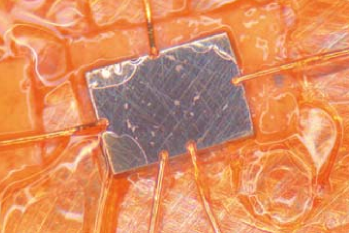
Figure 8: Photograph of a single crystal YbRh₂Si₂ contacted for magnetotransport measurements. The sample size is about $0.87\times 0.6$ mm², with a thickness of about 65 $\mu$m.

signal-to-noise ratio, the sample temperature needs to be monitored carefully.

A similar predicament holds for the magnitude of the magnetic field. From eq. (1), high fields appear preferable. However, it is typically the regime of linear response, i.e. the initial slope of $\rho_{\text{H}}$, one is interested in, see discussion of eq. (35) below and Fig. 12 for an example. This constrain often limits the magnitude of $B_{z}$.

Any experimental setup to be used for Hall measurements on metals has to be optimized for the measurement of small voltages. Besides careful cabling we fund the usage of low-temperature transformers [171] extremely helpful. These transformers allow for an impedance change (we typically amplify the voltage by a factor of 100) very close to the sample and at low temperatures, i.e. at low noise level. As a disadvantage, however, these transformers require magnetic field-free conditions provided by their superconducting housing and hence, the magnet used for Hall measurements must have a compensated zone. If Hall effect and magnetoresistance are to be measured simultaneously two transformers need to be implemented making space in a dilution refrigerator insert tight. Further amplification is provided by low-noise voltage [172] and, subsequently, lock-in amplifiers. The setup retains phase control over the ac signals which is of utmost importance for crosschecks on the measured Hall voltage.

A careful look at the sample contacts in Fig. 8 reveals an issue of far-reaching consequences: The voltage contacts are usually not perfectly aligned perpendicularly with respect to current $I_{x}$ (in contrast to patterned films). This misalignment causes a magnetoresistive component as part of the measured voltage $V_{\text{meas}}(B)=V_{y}(B)+V_{x}(B)$. To separate the two components one can make use of the fact that the Hall effect is antisymmetric, $V_{y}(B)=-V_{y}(-B)$, whereas the magnetoresistive part is symmetric, $V_{x}(B)=V_{x}(-B)$. Experimentally, this requires to measure $V_{\text{meas}}(B)$ at positive and negative magnetic fields, doubling the effort. The Hall voltage is then obtained by $V_{y}(B)=\frac{1}{2}[V_{\text{meas}}(B)-V_{\text{meas}}(-B)]$. As an important way of crosschecking on our results we regularly compare $V_{x}(B)=\frac{1}{2}[V_{\text{meas}}(B)+V_{\text{meas}}(-B)]$ to the directly measured (e.g. via the two lower contacts in Fig. 8) magnetoresistive voltage; these two voltages are related by a simple factor which only depends on sample geometry but not on magnetic field.

For Hall measurements on samples of irregular shape one can use the so-called van der Pauw method [173] provided the sample is of homogeneous thickness and of platelet-like form, i.e., much thinner then wide. Four contacts are attached at arbitrary positions on the circumference of the sample, as illustrated in Fig. 9. The van der Pauw method is handy for tiny samples like those used in diamond anvil pressure cells. The Hall voltage is extracted from two subsequent measurement protocols: First, the current is passed through one set of opposing contacts (e.g., 1 and 3 in the figure) with the voltage measured on the transverse contacts ($V_{24}$ in the figure). In a second step, the former voltage contacts (2 and 4) are used to inject the current and the voltage is measured on the former current contacts, giving again the transverse voltage ($V_{13}$ in the figure). The Hall voltage is calculated as $V_{\text{H}}=(V_{13}+V_{24})/2$. An often applied procedure to

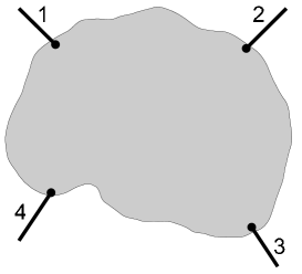
Figure 9: Sketch of a sample with contacts for van der Pauw measurements. An arbitrarily shaped sample of uniform thickness is connected via four contacts on its circumference. The resulting Hall voltage is obtained by swapping the contacts for current and voltage (see text).

separate magnetoresistivity contributions arising from the arbitrary distribution of the contacts is via the determination of the antisymmetric component of the Hall voltage under field reversal.

The vectorial nature of the ingredients as described in section 4.2.1 calls for a tensor notation in defining the primary quantities of interest, specifically the resistivity $\varrho$. Then, the Hall coefficient is given by $R_{\rm H}=[\varrho_{yx}(B)-\varrho_{xy}(-B)]/2B$. Though it is the Hall resistivity $\varrho_{xy}$ which is always measured in an experiment, it is common practice to report experimental data in the form of the Hall conductivity $\sigma_{xy}$ using a full matrix inversion, i.e., $\sigma_{xy}=\varrho_{xy}/[\varrho_{xx}^{2}+\varrho_{xy}^{2}]$. Considering the fact that there is no preferred choice of notation in literature, this review uses both these quantities interchangeably while describing prior data. Note that this requires the knowledge of both, $\varrho_{xx}$ and $\varrho_{xy}$ which is ideally measured simultaneously. Along the same lines we will use the notations $H$ and $B$ interchangeably to denote the magnetic field.

4.2 Advanced aspects of Hall effect measurements

4.2.1 Single-field Hall experiments

The traditional setup for Hall effect measurements was already sketched in Fig. 3. In the following we will refer to this as the single-field Hall setup with a single magnetic field $B_{1}$ being applied, in an effort to distinguish it from the crossed-field Hall setup discussed later, cf. section 4.2.2 and Fig. 10.

For a more general derivation of the Hall voltage, eq. (1), we consider the geometry shown in Fig. 3 and specify the boundary conditions as

$${\boldsymbol{j}}=\begin{pmatrix}j_{x}\\ 0\\ 0\end{pmatrix} {\boldsymbol{E}}=\begin{pmatrix}E_{x}\\ E_{y}\\ 0\end{pmatrix} {\boldsymbol{B}}=\begin{pmatrix}0\\ 0\\ B_{1}\end{pmatrix}$$ (31)

with the current density ${\boldsymbol{j}}$, the electrical field ${\boldsymbol{E}}$, and the magnetic field vector ${\boldsymbol{B}}$. The conductivity tensor defined via Ohm’s law as

$${\boldsymbol{j}}=\underline{\sigma}{\boldsymbol{E}}$$ (32)

relates the current and the electrical field and incorporates dependencies of its elements on the magnetic field ${\boldsymbol{B}}$. In the presence of one magnetic field in the $z$-direction only one may reduce the conductivity tensor to a $2\times 2$ form. By further taking into account the Onsager relations $\sigma_{xy}(B_{1})=-\sigma_{yx}(B_{1})$ [174, 175] and assuming an isotropic material with $\sigma_{xx}=\sigma_{yy}=\sigma$, one derives a tensor with two independent components

$$\underline{\sigma}=\begin{pmatrix}\sigma&\sigma_{xy}\\ -\sigma_{xy}&\sigma\\ \end{pmatrix}\,.$$ (33)

We note that moderate anisotropies may be incorporated without altering the main result. In order to obtain an expression for the Hall coefficient we calculate the resistivity tensor

$$\underline{\rho}=\begin{pmatrix}\rho&-\rho_{xy}\\ \rho_{xy}&\rho\\ \end{pmatrix}=\frac{1}{\sigma^{2}+\sigma_{xy}^{2}}\begin{pmatrix}\sigma&-\sigma_{xy}\\ \sigma_{xy}&\sigma\\ \end{pmatrix}\,.$$ (34)

The Hall resistivity $\rho_{\rm H}$ is identical to the element $\rho_{xy}$ as this element reflects the relation of the transverse electrical field to the longitudinal current corresponding to the definition of the Hall coefficient. We are now in the position to generalize eq. (1) and obtain the linear-response Hall coefficient as the corresponding element of the tensor on the right hand side of eq. (34)

$$R_{\text{H}}(B_{1})=\lim\limits_{B_{1}\to 0}\frac{\rho_{\text{H}}}{B_{1}}=\lim\limits_{B_{1}\to 0}\frac{1}{B_{1}}\frac{\sigma_{xy}}{\sigma^{2}+\sigma_{xy}^{2}}\approx\lim\limits_{B_{1}\to 0}\frac{1}{B_{1}}\frac{\sigma_{xy}}{\sigma^{2}}\;.$$ (35)

The last approximation originates from the fact that the Hall conductivity in metals is typically several orders of magnitude smaller as the normal conductivity, i.e., $\sigma_{xy}\ll\sigma$.

In accordance with eq. (35), the Hall coefficient is normally measured isothermally as the initial linear slope of the Hall resistivity with respect to the magnetic field. For simple metals the Hall coefficient is a constant which implies that the Hall resistivity is proportional to the magnetic field, $\rho_{\text{H}}\propto B_{1}$, cf. eq. (1). From this equation it is also obvious that the Hall coefficient $R_{\text{H}}$ reflects the effective charge carrier concentration which, for simple metals, does not depend on magnetic field.

However, for the investigation of more complex materials and/or phenomena such as quantum phase transitions the focus is often on non-linear effects. For the study of quantum criticality we are interested in metals which possibly change their Fermi surface topology and hence, also the effective charge carrier concentration. If this change is induced by a magnetic field, this will lead to a non-linearity in the Hall resistivity. The overall magnetic field $B_{1}$ applied will result in a tuning effect (cf. section 2.5) whereas the probing of the Fermi surface at this particular field strength shows up as the response to infinitesimal fields $\partial B_{1}$ (see Fig. 10(a)). It is therefore straightforward to define the differential Hall coefficient as

$$\tilde{R}_{\text{H}}(B_{1})=\frac{\partial\rho_{\text{H}}}{\partial B_{1}}\Big{|}_{B_{1}}$$ (36)

which allows to monitor the evolution of the Hall response across a field-induced QCP. Hence, the disentanglement of the two effects of the magnetic field might be done in the subsequent analysis by numerical differentiation as we shall see below.

Based on linear response theory one may analyze the differential Hall coefficient in more detail. The orbital deflection of the charge carriers in an external magnetic field introduced by the Lorentz force leads to a term which represents a generalized definition of the Hall coefficient:

$$R_{\text{H}}(B_{1})=\left[\frac{\partial\rho_{\text{H}}(B_{1})}{\partial B_{1}}\right]_{\text{orb}}$$ (37)

In a simple metal the Lorentz force is just proportional to the external magnetic field giving rise to a constant $R_{\text{H}}$ as expected. This orbital contribution corresponds to the probe in

single field	crossed field
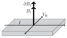
(a)	(b)

Figure 10: Hall effect setups to study field-induced QCPs. (a) Single-field setup with one magnetic field $B_{1}$. (b) Crossed-field setup with the additional magnetic field $B_{2}$.

our experiment, i.e., to the Hall response. When the Fermi surface topology changes, this is reflected in a change of the orbital contribution.

For the investigation of materials in which the ground state is field tuned, a second response to an external magnetic field arises, which is termed Zeeman term. Consequently, the differential Hall coefficient reflects both the orbital and the Zeeman contribution:

$$\tilde{R}_{\text{H}} =\left[\frac{\partial\rho_{\text{H}}(B_{1})}{\partial B_{1}}\right]_{\text{orb}} +\left[\frac{\partial\rho_{\text{H}}(B_{1})}{\partial B_{1}}\right]_{\text{Zeemann}}$$

$$=R_{\text{H}}(B_{1}) +\left[\frac{\partial\rho_{\text{H}}(B_{1})}{\partial B_{1}}\right]_{\text{Zeemann}}\;.$$ (38)

We used eq. (37) to relate the first term to a linear-response of the system. The Zeeman term is not known to be related to any measurable linear-response quantity. Consequently, it is not straight forward to interpret results of the single-field Hall experiment.

4.2.2 Crossed-field Hall experiments

The recent interest in heavy-fermion systems stems mainly from their model character in the investigation of QCPs. Although being phase transitions at zero temperature quantum critical points lead to unusual properties up to surprisingly high temperatures. This issue becomes particularly apparent for the cuprate superconductors for which quantum criticality is also discussed (see, e.g. [102] and section 7.1.1). We shall see that the Hall effect turned out to be a sensitive tool to explore the nature of a particular QCP.

Hall effect measurements provide currently the best probe to study the Fermi surface evolution at quantum critical points. This is mainly due to the experimental difficulties associated with other probes: ARPES is limited to higher temperatures (compared to magnetotransport experiments) whereas quantum oscillation measurements can only be conducted in a range of high magnetic fields and on very clean samples.

In order to distinguish whether the Fermi surface evolves continuously or discontinuously one needs to have sufficient resolution of the control parameter used to access the quantum critical point. As the heavy-fermion systems involve magnetic interactions, magnetic field tuning is the obvious choice to achieve such high resolution. This, however, means that the magnetic field has to cover two tasks, namely, tuning the material across its QCP and probing its Fermi surface by generating a Hall voltage. Two different approaches can be pursued to disentangle these two effects.

Firstly, the conventional, single-field Hall effect setup as described in section 4.2.1 might be employed. Here, the tuning effect stems from the overall applied magnetic field $B_{1}$ whereas the probing of the Fermi surface at this particular field strength shows up as the response to infinitesimal fields, see Fig. 10(a). The differential Hall coefficient $\tilde{R}_{\text{H}}$ is given by eq. (36) and can be related to the Fermi surface via the Kubo formalism [176]. Hence, the disentanglement of the two effects exerted by the magnetic field $B_{1}$ is done in the subsequent analysis by numerical differentiation.

Secondly, by using two magnetic fields one can disentangle the two tasks already within the measurement. In order to do so, one magnetic field $B_{1}$ is applied perpendicular to the current to generate the Hall response whereas the second magnetic field $B_{2}$ is directed parallel to the current to tune the material, as sketched in Fig. 10(b). We refer to this as crossed-field Hall effect setup. One precondition for this disentanglement to successfully work out is, however, that the tuning effect arising from $B_{1}$ has a negligible tuning effect to the material under investigation compared to the tuning field $B_{2}$. If the material exhibits a sufficiently high magnetic anisotropy it can be utilized to ensure this condition. An influence of $B_{2}$ on the Hall effect is generally small as it is parallel to the current avoiding a Lorentz force acting on the electrons. Consequently, tuning of the material is predominantly achieved by $B_{2}$ whereas the Hall effect stems from $B_{1}$. The power of the crossed-field setup lies in the fact that the Hall effect represents the linear response of the system with respect to the Hall field $B_{1}$: The Hall coefficient is extracted as the initial slope of the Hall resistivity at a fixed tuning field $B_{2}$,

$$R_{\text{H}}(B_{2})=\lim_{B_{1}\to 0}\frac{\rho_{\text{H}}(B_{1},B_{2})}{B_{1}}\;.$$ (39)

If the geometry between Hall field $\partial B_{1}$, Hall voltage and injected current is kept identical for both the single-field and the crossed-field configurations, the orbital contribution of the differential Hall coefficient $R_{\text{H}}(B_{1})$ and the linear-response Hall coefficient $R_{\text{H}}(B_{2})$ respond to the evolution of the Fermi surface. Differences may be ascribed to the Zeeman term or magnetic anisotropies as discussed below and in section 5.1.

We shall scrutinize the influence of $B_{2}$ on the Hall response arising from $B_{1}$ by analyzing the conductivity tensor for this setup. For the given geometry the boundary conditions may be framed as

$${\boldsymbol{j}}=\begin{pmatrix}j_{x}\\ 0\\ 0\end{pmatrix} {\boldsymbol{E}}=\begin{pmatrix}E_{x}\\ E_{y}\\ 0\end{pmatrix} {\boldsymbol{B}}=\begin{pmatrix}B_{2}\\ 0\\ B_{1}\end{pmatrix}$$ (40)

Clearly, the conductivity tensor $\underline{\sigma}$ relating the current density and the electrical field via eq. (32) will be a $3\times 3$ matrix. Only the elements $\sigma_{xz}=\sigma_{zx}=0$ can be omitted as no magnetic field is applied in $y$-direction. Taking advantage of the Onsager relations [174, 175] one derives

$$\underline{\sigma}=\begin{pmatrix}\sigma_{xx}&\sigma_{xy}&0\\ -\sigma_{xy}&\sigma_{yy}&\sigma_{yz}\\ 0&-\sigma_{yz}&\sigma_{zz}\\ \end{pmatrix}$$ (41)

The resistivity tensor $\underline{\rho}$ may again be derived via inversion

$$\underline{\rho}=\frac{1}{\sigma_{xx}\sigma_{yy}\sigma_{zz}+\sigma_{yz}^{2}\sigma_{xx}+\sigma_{xy}^{2}\sigma_{zz}}\begin{pmatrix}\sigma_{yy}\sigma_{zz}+\sigma_{yz}^{2}&-\sigma_{xy}\sigma_{zz}&0\\ \sigma_{xy}\sigma_{zz}&\sigma_{zz}\sigma_{xx}&-\sigma_{yz}\sigma_{xx}\\ 0&\sigma_{yz}\sigma_{xx}&\sigma_{xx}\sigma_{yy}+\sigma_{xy}^{2}\\ \end{pmatrix}$$ (42)

from which the Hall coefficient can be read off as

$$R_{\text{H}}=\lim\limits_{B_{1}\to 0}\frac{\rho_{xy}}{B_{1}}=\lim\limits_{B_{1}\to 0}\frac{1}{B_{1}}\frac{\sigma_{xy}}{(\sigma_{xx}\sigma_{yy}+\sigma_{yz}^{2}\sigma_{xx}\sigma_{zz}^{-1}+\sigma_{xy}^{2})}\;.$$ (43)

Rearranging eq. (43) allows a detailed comparison to the single-field case ($B_{2}=0$):

$$R_{\text{H}}=\lim\limits_{B_{1}\to 0}\frac{1}{B_{1}}\frac{\sigma_{xy}}{\sigma_{xx}\sigma_{yy}+\sigma_{xy}^{2}}\left(1+\frac{\sigma_{yz}^{2}}{\sigma_{xx}\sigma_{zz}}\right)^{-1}\approx\frac{1}{B_{1}}\frac{\sigma_{xy}}{\sigma^{2}}\left(1+\frac{\sigma_{yz}^{2}}{\sigma^{2}}\right)^{-1}\;.$$ (44)

For the approximation in eq. (44) the same symmetry simplification as for the case of the single-field Hall experiment, $\sigma_{xx}\approx\sigma_{yy}$ and the assumption of $\sigma_{xy}\ll\sigma_{xx}$ are used. Again, incorporating moderate anisotropies does not alter the results. In fact, it will become clear that one might utilize anisotropies to enable higher resolution in the crossed-field Hall experiment.

The leading contribution to $R_{\text{H}}$ in eq. (44) stems from the unity within the sum and matches the result of the single-field Hall experiment, eq. (35). This contribution corresponds to the Hall constant in a gedanken setup in which the field $B_{2}$ does not generate any Lorentz force while fulfilling the role of tuning the underlying state. The second part of the sum, $\frac{\sigma_{yz}^{2}}{\sigma^{2}}$, represents a correction to this case. In order to obtain an estimate for this correction we ignore anisotropies in the material, i.e., we assume that the off-diagonal elements of the conductivity tensor are similar: $\sigma_{yz}\approx\sigma_{xy}$. Thereby we derive that the correction to the ideal case without any direct effect of $B_{2}$ on the Hall coefficient is given by

$$\frac{\sigma_{yz}^{2}}{\sigma_{xx}\sigma_{zz}}\approx\left(\frac{\rho_{\text{H}}}{\rho}\right)^{2}\ll 1\;.$$ (45)

We estimate this correction to be much smaller than 1 using again that for metals the off-diagonal elements of the conductivity tensor are typically several orders of magnitude smaller than the diagonal elements. Equation (45) denotes the square of the tangent of the Hall angle $(\tan\theta_{\text{H}})^{2}$ which is typically of the order of $10^{-4}$ for metals at low temperatures and small fields. Consequently, this correction may be neglected.

These considerations of the transport theory emphasize that the single-field Hall setup allows to study the Hall effect evolution across a QCP by means of the differential Hall coefficient which is composed of an orbital response and a Zeeman term. By contrast, the crossed-field Hall experiment exclusively yields the linear-response Hall coefficient associated with the orbital effect. Consequently, the crossed-field Hall setup appears to be superior. However, we shall see that the crossed-field setup is experimentally more demanding. The consistency of the two setups was tested by investigating a non-magnetic metal [177], see section 4.2.4.

4.2.3 Realization of crossed-field Hall experiments

For many investigations access to lowest possible temperatures is desired or even required. Hence, Hall effect measurements are often performed in a ³He/⁴He-dilution refrigerator. For the case of the crossed-field Hall setup a vector magnet comprising at least to components is favorable. Such a setup is sketched in Fig. 11. Here, the Hall field $B_{1}$ is generated by a solenoid oriented vertically whereas the tuning field $B_{2}$ is generated by a split pair oriented horizontally. Superconducting magnets in persistent mode allow low noise measurements of the Hall signal.

This setup is clearly superior to an earlier realization of crossed fields [176] in which a miniature superconducting coil (providing $B_{2}$) was mounted inside a dilution refrigerator equipped with a conventional solenoidal superconducting magnet (used to apply $B_{1}$). In the latter case, problems arose due to the limited space (limiting the magnitude of $B_{2}$), possible quenching of the miniature coil and a difficult alignment of the coils and the sample. We note that the tuning field $B_{2}$ should be adjustable.

The Hall voltage is measured as a function of $B_{1}$ at several field strengths of $B_{2}$. This allows to extract the Hall coefficient $R_{\text{H}}(B_{2})$ as the initial linear slope of the Hall resistivity $\rho_{\text{H}}$ with respect to $B_{1}$ at fixed $B_{2}$, cf. eq. (39). Again, the Hall voltage is to be measured at negative and positive fields $B_{1}$ to enable the analysis of the antisymmetric part (cf. section 4.1). As we shall see below it is favorable to measure also at positive and negative $B_{2}$ to correct for misalignments. Consequently, the Hall voltage has to be scanned on a close mesh of $B_{1}$ and $B_{2}$ (and $T$ in order to allow an extrapolation to $T\to 0$). The effort is partially reduced by the fact that it is sufficient to restrict the range of $B_{1}$ to small fields as we are only interested in the initial slope of $\left.\rho_{\text{H}}(B_{1})\right|_{B_{2}}$. The second magnetic field $B_{2}$, however, gives rise to a large increase in measurement time.

The experimental procedure is illustrated in Fig. 12 for the measurements on YbRh₂Si₂ at one particular temperature ($T=65$ mK). Here, the Hall resistivity vs. $B_{1}$ clearly

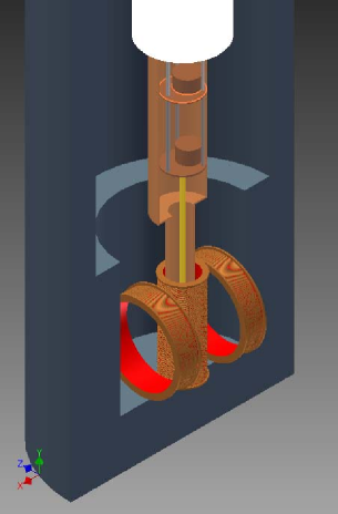
Figure 11: Experimental realization of the crossed-field Hall setup. A ³He/⁴He-dilution refrigerator is combined with a vector magnet comprising a solenoid generating a field in the vertical direction and a split pair generating a horizontal magnetic field, parallel to the current injected into the sample (not shown).

exhibits a linear field dependence. Importantly, however, the slope of these curves, i.e. $R_{\text{H}}$, is different for different tuning fields $B_{2}$. The slope of $\rho_{\text{H}}(B_{1})$ was extracted from least square fits to determine the dependence of $R_{\text{H}}(B_{2})$. This is to be done for several temperatures in order to enable an extrapolation to zero temperature.

For the conduction of the crossed-field Hall experiments it is necessary to keep the tasks of the magnetic fields well separated. As already pointed out, the tuning effect of the Hall field $B_{1}$ should be small compared to the tuning effect of the tuning field itself. This may be assured by applying small field $B_{1}$ only, but this also decreases the Hall signal and hence, the sensitivity. Note that also for the single-field Hall setup one is faced with this issue. For a material with a small critical field it will be hard to resolve non-linear effects as the Hall signal will be small around the critical field. Large critical fields on the other hand will lead to an increase of the Zeeman response in the single-field Hall setup and might easily be beyond the field scale accessible with vector magnets needed for the crossed-field Hall setup.

One may partially overcome the above described issues by taking advantage of anisotropies in the materials response to external fields. For the case of YbRh₂Si₂ which is discussed in more detail in section 5.1, the magnetic anisotropy is such that a

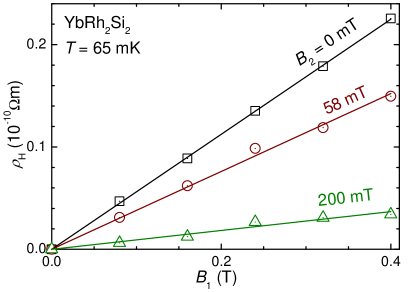
Figure 12: Exemplary Hall resistivity isotherms for one YbRh₂Si₂ sample. Solid lines mark linear fits to the data with the slope of these lines corresponding to the linear-response Hall coefficient $R_{\text{H}}$.

field along the crystallographic $c$ direction has to be 11 times larger compared to a field within the crystallographic $ab$ plane to generate the same tuning effect on the ground state of the material. Clearly, this favors an application of the Hall field $B_{1}$ along the $c$ direction and, thus, in the case of the crossed-field experiment, the tuning field $B_{2}$ within the easy $ab$ plane. This allows to use higher fields $B_{1}$ inducing larger Hall voltages without generating a substantial tuning effect. In the case of YbRh₂Si₂ it turned out that fields $B_{1}\lesssim 0.4$ T could be used without disturbing the tuning effect generated by $B_{2}$. In fact, the Hall resistance remained linear also in proximity to the critical value of the tuning field where the Hall coefficient $R_{\text{H}}(B_{2})$, and thus the slope of the Hall resistivity considerably changes, as can be seen from Fig. 12.

One of the major issues of the experimental setup as depicted in Fig. 11 is the alignment of the magnetic fields with respect to the sample. This appears to be an issue for both the single-field and crossed-field Hall setup as misalignments can lead to unwanted effects. For the single-field Hall setup it is important to have a precise alignment of $B_{1}$ perpendicular to the current and to the Hall voltage contacts. Any component out of this plane will generate a tuning effect without inducing a Hall response. This effect will be amplified by a magnetic anisotropy. However, one may take advantage of the magnetic anisotropy to align the sample with respect to the magnetic field (or vice versa). A proper orientation may be assured by monitoring characteristic features related to the materials response to magnetic fields as a function of angle between sample and magnetic field. For the experiments on tetragonal YbRh₂Si₂ a precision of better than $0.5^{\circ}$ in alignment of $B_{1}$ parallel to the magnetic hard $c$ direction was achieved by maximizing the critical field while rotating the sample with respect to the field direction [178].

For the crossed-field Hall setup a misalignment might lead to a mixing of the intended effects of the two magnetic fields. Any component of $B_{1}$ within the plane of the current and Hall voltage contacts acts as a tuning field, and a component of $B_{2}$ perpendicular to current and Hall voltage contacts contributes to the Hall field $B_{1}$. Even small misalignments of the order of $1^{\circ}$ may change the results dramatically in the presence of a magnetic anisotropy (as in case of YbRh₂Si₂). In fact, a tilting of the sample may lead to an antisymmetric part in the longitudinal voltage as a function of $B_{1}$ if $B_{2}$ is finite. This is in contrast to the fact that the longitudinal resistivity, i.e., the magnetoresistance $\rho_{xx}(B)$ is a symmetric function of magnetic field. This effect arises solely from the non-trivial combination of the two magnetic fields. For the measurement of the Hall coefficient in the crossed-field setup this is crucial because a longitudinal component will be present on the Hall voltage contacts as well. This component is usually separated by taking the antisymmetric part of the measured voltage to derive the Hall resistivity. This, however, fails if the longitudinal component already contains an antisymmetric part due to sample misalignment. Such an antisymmetric part would consequently add to the Hall coefficient. As a sample is manually aligned to a precision of the order of several degree only one might correct such a misalignment by tilting back the data. For the experiments on YbRh₂Si₂, the uncertainty could be reduced to a tilting in the plane spanned by $B_{1}$ and $B_{2}$. Consequently, it was possible to analytically rotate back the Hall voltage $V_{\text{H}}(B_{1},B_{2})$. Therefore, both the longitudinal voltage $V_{x}$ and the Hall voltage $V_{y}$ were measured simultaneously as a function of $B_{1}$ and $B_{2}$, with $B_{2}$ ranging from positive to negative values. The analysis of the longitudinal voltage revealed an antisymmetric component which could be omitted when rotating the data by a small angle. The Hall voltage was then corrected by the same angle prior to the calculation of the Hall resistivity and the Hall coefficient [178].

4.2.4 Comparison of single and crossed-field Hall experiments

The consistency of the single-field and crossed-field Hall setup was checked for a non-magnetic metal, LuRh₂Si₂ [177]. In these two measurements a linear decrease of the differential and linear-response Hall coefficient was revealed, respectively. The comparison of the results is illustrated in Fig. 13. First, the single-field Hall results (open symbols) display a linear decrease as the magnetic field is increased up to $B_{1}=1$ T. Above this field a saturation gradually sets in. Second, in the crossed-field Hall experiment a linear decrease of $R_{\text{H}}(B_{2})$ is observed over the complete field range studied, i.e., up to $B_{2}=4$ T. The fact that the change of the Hall coefficient is linear in both experiments suggests a Zeeman splitting of the Fermi surfaces as the underlying mechanism. The different field range over which the linearity occurs might be related to the anisotropy of the material: $B_{1}$ and $B_{2}$ are applied along different crystallographic directions. In fact, the data collapse if the crossed-field Hall data are scaled by $B_{2}/B_{1}=4$ (note that the anisotropy in LuRh₂Si₂ is not only smaller than in YbRh₂Si₂ but also reversed). The different

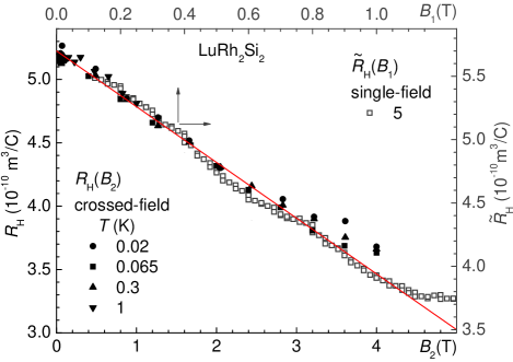
Figure 13: Comparison of crossed-field and single-field Hall coefficient of LuRh₂Si₂Ċrossed-field results $R_{\text{H}}(B_{2})$ are plotted on the lower and left axis, whereas single-field results $\tilde{R}_{\text{H}}(B_{1})$ are plotted on the upper and right axis. Solid line emphasizes the linear evolution of both at small fields. The field axis of the single-field data is scaled by a factor of 4 with respect to the crossed-field data accounting for the anisotropy observed in the field dependence of the Hall coefficient. In addition, the ordinate of the crossed-field data is shifted by ${0.475\times 10^{-10}}$ m³/C compensating the reduction of $R_{\text{H}}$ in the crossed-field experiment (see text). Reproduced with permission from S. Friedemann et al., Physica Status Solidi B 247 (2010) 723 [177]. Copyright © 2010 WILEY-VCH.

temperatures of the crossed-field and single-field Hall data do not affect these considerations as both crossed-field and single-field Hall results do not exhibit any temperature dependence below 20 K.

In the crossed-field experiment, the Hall field $B_{1}$ also influences the tuning of the system due to the unfavourable anisotropy. Therefore, a disentanglement of the two effects of the magnetic field is incomplete in contrast to the case of YbRh₂Si₂, as we shall see in section 5. In fact, the results on LuRh₂Si₂ in the crossed-field configuration demonstrate that the tuning effect can arise from both the dedicated tuning field $B_{2}$ as well as from the Hall field $B_{1}$. Here, the Hall coefficient is deduced as the positive linear slope of the Hall resistivity over a finite field range. In this field range, however, the Hall resistivity is sublinear as best seen from the decrease of the differential Hall coefficient (see Fig. 13). Consequently, the slope of the linear fits and thus the linear-slope Hall coefficient reflects an average of the differential Hall coefficient over the field range considered for the linear fits. This leads to a reduction of the linear-slope Hall coefficient with respect to the differential Hall coefficient which is reflected in Fig. 13 as a negative offset of the crossed-field Hall results. This confirms that for the case of LuRh₂Si₂ in the crossed-field Hall experiment tuning stems from both $B_{2}$ and $B_{1}$. The tuning contribution of $B_{1}$ can be minimized by either going to smaller fields $B_{1}$ which makes the Hall signal harder to detect, or by utilizing magnetic anisotropies such as described for YbRh₂Si₂.

This section reveals the experimental difficulties associated with the two setups. Although one should not underestimate the issues of the single-field Hall setup, the crossed-field experiment is much more involved. In case of the single-field setup (which is very much established for the investigations of quantum critical phenomena) one should consider the effort of low-temperature measurements and precise orientation. For the crossed-field Hall setup the effort is extended by the additional magnet needed and the time consumption to scan the second magnetic field. However, due to the difficulties with the interpretation of the single-field Hall results it is necessary to combine them with crossed-field Hall measurements. As we shall see in section 5.1, the crossed-field Hall effect measurements seem to be the superior probe to reveal a Fermi surface reconstruction at a QCP.

5 Hall effect and Kondo-breakdown quantum criticality

5.1 Hall effect evolution at the QCP in YbRh₂Si₂

The heavy-fermion material which was very extensively studied by Hall effect measurements across its QCP is YbRh₂Si₂. We discuss the results on this material and subsequently compare to other heavy-fermion materials. Hall effect measurements on YbRh₂Si₂ provide currently the best evidence for a Fermi surface reconstruction at a QCP. In fact, these Hall effect measurements allowed also to extract information on the quantum critical scaling behavior as we shall see below.

YbRh₂Si₂ is a prototypical material for the investigation of quantum critical phenomena. The heavy-fermion character is evident from various transport and thermodynamic properties. The resistivity $\rho$ exhibits a logarithmic temperature dependence above 100 K associated with the single ion Kondo scattering. Below 100 K, $\rho(T)$ [179, 180] as well as the thermopower [180] decrease as the temperature is reduced reflecting the onset of coherent Kondo scattering and the formation of composite quasiparticles. These effects, however, involve all crystalline electric field (CEF) levels [181]. Upon cooling, the 4$f$ electrons increasingly “condense” into their CEF-derived Kramers doublet ground state allowing the formation of a Kondo lattice below around 30 K [179, 180]. These effects of combined CEF and Kondo interactions have recently been demonstrated by scanning tunneling spectroscopy on YbRh₂Si₂ [182]. Only at very low temperatures of $T_{\text{N}}=70$ mK orders YbRh₂Si₂ antiferromagnetically [179]. The Néel temperature $T_{\text{N}}$ is continuously suppressed by a small magnetic field leading to the QCP. This field-induced QCP is accessed at a critical field of either $B_{1\text{c}}=660$ mT if applied along the crystallographic $c$ direction, or $B_{2\text{c}}=60$ mT if applied perpendicular to the $c$ axis. This magnetic anisotropy is used to the advantage of separating the two magnetic field tasks in the crossed-field experiment (cf. 4.2.3). The phase transition appears to remain continuous down to at least 15 mK [183] indicating gapless quantum fluctuations. Right at the critical field pronounced non-Fermi liquid behavior is observed over three decades in temperature down to the lowest temperatures accessible [184]. This non-Fermi liquid behavior is best explained to arise from the quantum fluctuations within the QCP picture which assumes a continuous phase transition at zero temperature. The non-Fermi liquid behavior comprises a logarithmic divergence of the Sommerfeld coefficient of the electronic specific heat, i.e. $\gamma=C_{\text{el}}/T\propto\log(T/T_{0})$, and a linear temperature dependence of the resistivity [179, 184]. At fields larger than the critical field a Fermi liquid ground state is recovered. Here, the resistivity follows a quadratic temperature dependence and the Sommerfeld coefficient saturates. The characteristics of this Fermi liquid phase are strongly enhanced as typical for a heavy fermion material, the quadratic coefficient of the resistivity and the Sommerfeld coefficient obey values up to a factor 1000 larger than in non-correlated metals [184]. This reflects an extremely large effective mass of the composite quasiparticles.

Indications of an unconventional type of quantum criticality arose from measurements of the Grüneisen ratio [185]. The temperature dependence of the Grüneisen ratio strongly underpins the presence of a QCP as it obeys a power-law divergence, i.e., $\Gamma\propto T^{-x}$. The observed exponent of $x=0.7$ is, however, in contrast to the predictions of the conventional SDW QCP ($x=1$). This fact along with the outcome of $B/T$ scaling of both the specific heat and the electrical resistivity [7] suggests that YbRh₂Si₂ is an ideal candidate for unconventional quantum criticality. This motivated extensive Hall effect studies on YbRh₂Si₂ [176, 53]. As the Hall coefficient is a rather complex quantity in its relation to the Fermi surface (cf. section 2.4) we should first note some peculiarities of the Hall effect in YbRh₂Si₂. First, the anomalous Hall effect is shown to be dominant at high temperatures but is negligible at lowest temperatures [186]. In addition, we shall see that the anomalous Hall contributions can not account for the signatures related to quantum criticality. Second, we note that the low temperature Hall coefficient of YbRh₂Si₂ is found to exhibit sample dependencies. For the almost compensated two-band material YbRh₂Si₂ these sample dependencies where found to arise from slight changes of the relative scattering rates of the two dominating bands [187]. These differences in the relative scattering rates appear to originate from tiny variations in the composition because they only affect samples from different batches. A systematic study of different samples revealed the sample dependencies to be associated with a background contribution whereas the contributions related to the quantum criticality are robust [53].

The Hall effect on YbRh₂Si₂ was studied in both the single-field and the crossed-field geometry (explained in section 4.2). These studies are further corroborated by longitudinal magnetoresistance measurements (see Ref. [49]). In the single-field Hall experiment, a single magnetic field, $B_{1}$, applied along the $c$ axis was used to both tune and probe the sample. For the crossed-field Hall experiment, the tuning was carried out with an additional magnetic field $B_{2}$ within the crystallographic $ab$ plane while a small field $B_{1}$ was utilized to probe the system. The scales of the tuning fields, i.e., $B_{1}\parallel c$ and $B_{2}\perp c$, of the two experiments differ by the magnetic anisotropy of the material. This is quantified by the ratio of the critical fields $B_{2\text{c}}/B_{1\text{c}}=1/11$. We shall use this ratio to convert the single-field Hall results to the equivalent crossed-field scale. As detailed in section 4.2.2 the latter orientation allows to probe the system at larger fields $B_{1}$ thus increasing the Hall signal. Fig. 12 illustrates that in an extended range of low fields up to $B_{1}=0.4$ T, the Hall resistivity is linear with respect to $B_{1}$ even close to the

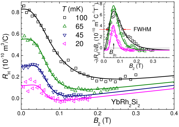
Figure 14: Crossed-field Hall effect results: Linear-response Hall coefficient measured in the crossed-field Hall experiment on YbRh₂Si₂. The field dependence of the isothermal linear-slope Hall coefficient is derived from linear fits to the Hall resistivity $\left.\rho_{\text{H}}(B_{1})\right|_{B_{2},T}$ as detailed in section 4.2.2 (Fig. 12). Solid lines are best fits of eq. (47) to the data extending up to 2 T. The inset shows the derivative $-\mathrm{d}R_{\text{H}}/\mathrm{d}B_{2}$ of both the data (symbols) and the fits (solid lines). Vertical arrow indicates the critical field $B_{2\text{c}}$. Horizontal arrows specify the FWHM of the peak for one curve. Reproduced from S. Friedemann et al., Proceedings of the National Academy of Science USA 107 (2010) 14547 [53].

critical field $B_{2\text{c}}$ which, in consequence, allows to reliably extract the linear-response Hall coefficient as a function of $B_{2}$. The longitudinal magnetoresistance as shown in detail in Ref. [49] was measured with field perpendicular to the $c$-axis simultaneous to the crossed-field Hall effect and is therefore associated with the equivalent field scale $B_{2}$.

Figs. 14 and 15 display selected isotherms of the linear-response Hall coefficient $R_{\text{H}}(B_{2})$ and the differential Hall coefficient $\tilde{R}_{\text{H}}(B_{1})$ deduced in the crossed-field and single-field Hall experiment, respectively. For plots of the magnetoresistance data we refer the reader to Ref. [49]. All data sets exhibit similar behavior comprising two main features. First, at small, increasing fields the Hall coefficient and the magnetoresistance decreases in a pronounced, crossover-like fashion. Second, at elevated fields and low temperatures, the crossover of the Hall coefficient is followed up by a linear increase. With decreasing temperature the crossover becomes sharper in field, decreases in height, and is shifted to lower fields in both experiments. In fact, it approaches the critical field in all cases, i.e., $B_{1\text{c}}$ and $B_{2\text{c}}$ for the single-field and crossed-field Hall and magnetoresistance experiment, respectively. Consequently, the crossover is related to the quantum critical behavior. With the crossover being restricted to small fields the linear behavior is revealed over an increasing field range as the temperature is lowered. This suggests that the linear behavior represents a background contribution to which the crossover is superposed. The linearity of the background contribution suggests that it originates from Zeeman splitting. Moreover, it is subject to the above mentioned sample dependencies. The main features of the curves, i.e. the crossover, by contrast, are not affected by the sample dependencies. The decomposition of the Hall coefficient into a critical and a background contribution is further illustrated in the inset of Fig. 14. Here, the derivative $-\partial R_{\text{H}}/\partial B_{2}$ is shown. The crossover is reflected by a peak around the critical field (indicated by a vertical arrow) whereas the background contribution appears as a non-zero offset. Below, we shall examine the characteristics of the crossover in the Hall coefficient in more detail and relate it to the quantum critical contribution.

An anomalous contribution to the Hall effect in YbRh₂Si₂ appears to be negligible at lowest temperatures. The skew scattering (cf. section 2.3.1)

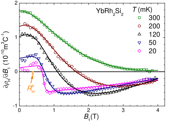
Figure 15: Single-field Hall effect results: Isotherms of the numerically derived differential Hall coefficient $\tilde{R}_{\text{H}}(B_{1})$ of YbRh₂Si₂. Solid lines mark best fits of eq. (47) to the data. The vertical bar denotes the size of the constant offset originating from an anomalous contribution estimated from eq. (46) via $R_{\text{H}}^{\text{a}}=\partial\rho_{\text{H}}^{\text{a}}/\partial B_{1}$. Reproduced with permission from S. Friedemann et al., Journal of Physics: Condensed Matter 23 (2011) 094216 [49]. Copyright (2011) IOP Publishing Ltd.

typically important in heavy fermion systems at high temperatures was found to lead to pronounced signatures in $R_{\text{H}}(T)$ around 100 K. At lowest temperatures, however, this contribution is largely suppressed. The fact that the anomalous contribution to the Hall resistivity

$$\rho_{\text{H}}^{\text{a}}(B_{1})=C\rho(B_{1})\mu_{0}M(B_{1})$$ (46)

is essentially linear in field implies that it adds a small constant offset to the Hall coefficient. Using the constant $C$ determined at higher temperatures [186] leads to a value of $\rho_{\text{H}}^{\text{a}}=0.07\times 10^{-10}$ m${}^{3}/$C which is tiny compared to the large variation of the differential Hall coefficient as illustrated by the vertical bar in Fig. 15. More importantly, the added offset to the Hall coefficient does not affect the analysis of the critical contribution. Particularly, the width, height and position of the crossover are independent of any offset.

For the detailed analysis the empirical function

$$R_{\text{H}}(B_{2})=R_{\text{H}}^{\infty}+mB_{2}-\frac{R_{\text{H}}^{\infty}-R_{\text{H}}^{0}}{1+(B_{2}/B_{0})^{p}}$$ (47)

was fitted to the data. This function simulates a crossover from the zero-field value $R_{\text{H}}^{0}$ to the high-field value $R_{\text{H}}^{\infty}$ superposed to a linear background $mB_{2}$. The position of the crossover is given by $B_{0}$ and the sharpness is determined by $p$ which is restricted to positive values. The function describes the data very well as can be seen from Figs. 14 and 15. Analogous fits to the differential Hall coefficient $\tilde{R}_{\text{H}}(B_{1})$ measured in the single-field experiment yielded the zero-field and high-field values $\tilde{R}_{\text{H}}^{\infty}$ and $\tilde{R}_{\text{H}}^{0}$, respectively. Equation (47) allows to deduce the characteristics of the crossover, i.e., the quantum critical contribution. In the following we shall focus on a complete characterization of the crossover with respect to its position, width and height.

Firstly, the position of the crossover is tracked in the phase diagram shown in Fig. 16 for two samples of very different values of the residual resistivity which span the whole range of sample dependencies observed for the low-$T$ Hall coefficient (cf. Ref. [187] with identical nomenclature). The crossover field is found to match for both samples and for three different experiments, i.e., for crossed-field and single-field Hall effect measurements and for the analogous crossover in the magnetoresistivity. As the temperature is lowered $B_{0}$ shifts to lower fields and converges to 60 mT, i.e., it extrapolates to the QCP in the limit of zero temperature. This reveals the linkage of the crossover in the

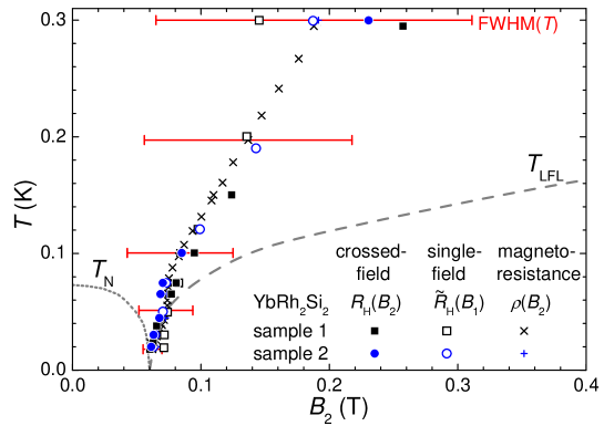
Figure 16: Linkage of the Hall crossover to the QCP in YbRh₂Si₂. The crossover field $B_{0}$ was extracted from fits of eq. (47) to the crossed-field $R_{\text{H}}(B_{2})$ (solid symbols) and single-field $\tilde{R}_{\text{H}}(B_{1})$ (open symbols) Hall results as shown in Figs. 14 and 15 as well as to magnetoresistance $\rho(B_{2})$ (Ref. [49]). Results on two samples with different residual resistivities match within experimental accuracy. The values deduced from the single-field Hall experiment are scaled by $1/11$ to account for the magnetic anisotropy of the material (see text). Red horizontal bars represent the FWHM at selected temperatures. Error bars are omitted to avoid confusion with the FWHM bars; with exception of the data at 0.3 K and the single-field result on sample 2 at 0.19 K standard deviations are smaller than the symbol size. Dotted and dashed lines mark the boundary of the magnetically ordered phase and Fermi-liquid regime, respectively, as taken from Ref. [184]. Reproduced from S. Friedemann et al., Proceedings of the National Academy of Science USA 107 (2010) 14547 [53].

Hall coefficient (and magnetoresistance) to the quantum criticality.

Secondly, the height of the crossover is characterized by the limiting parameters $R_{\text{H}}^{0}$ and $R_{\text{H}}^{\infty}$. Their temperature dependencies are plotted in Fig. 17 on a quadratic temperature scale which allows to identify important temperature dependencies as we shall see in the following. The absolute values of $R_{\text{H}}^{0}$ and $R_{\text{H}}^{\infty}$ differ for the two samples, in accordance with the sample dependencies that are associated with the background contribution to $R_{\text{H}}$. The quantum critical contribution is characterized by the difference $R_{\text{H}}^{0}-R_{\text{H}}^{\infty}$. This difference decreases as the temperature is lowered which can be seen from the $R_{\text{H}}(B_{2})$ curves in Fig. 14. In order to draw conclusions on the evolution of the Fermi surface at the QCP we need to deduce this difference in the limit $T\to 0$. Therefore, we utilize the temperature dependencies found for the initial-slope Hall coefficient. The zero-field value $R_{\text{H}}^{0}$ extracted from the fits matches very well with the measured initial-slope Hall coefficient in zero tuning field. We can therefore use the quadratic temperature dependence found for the initial-slope Hall coefficient below $T_{\text{N}}$ to reliably extrapolate to $T\to 0$ (cf. solid lines in Fig. 17) [49]. The temperature dependence of the high-field value $R_{\text{H}}^{\infty}$ is less pronounced and may well be approximated with a quadratic form as well. Importantly, the extrapolation of $R_{\text{H}}^{0}(T)$ and $R_{\text{H}}^{\infty}$ clearly indicates that their difference persists in the extrapolation $T\to 0$, i.e., down to the QCP. This is not only true for $R_{\text{H}}^{0}-R_{\text{H}}^{\infty}$ of both samples but also for the difference $\tilde{R}_{\text{H}}^{0}-\tilde{R}_{\text{H}}^{\infty}$ of the limiting values extracted from the single-field Hall experiment displayed in Fig. 17(b) as well as for the corresponding values of the crossover in magnetoresistance [49]. In summary, we can conclude that a change in the Hall coefficient persists at the QCP and is robust against sample dependencies.

The absolute value of the crossover height, $R_{\text{H}}^{0}-R_{\text{H}}^{\infty}$, is difficult to evaluate because multiple bands almost compensate each other at $E_{F}$ (despite the fact that the valence of $\sim$2.9 indicates YbRh₂Si₂ to be a hole system [188]) and these bands are influenced by sample dependencies [187]. Yet, the drop of $R_{\text{H}}$ at $B_{0}$ is consistent with a change from two hole-like Fermi-surface sheets dominating at $B<B_{0}$ to one hole/one electron sheet for $B>B_{0}$ due to the hybridization between 4$f$ and conduction electrons in the latter case.

Finally, we examine the width of the Hall crossover. This is accomplished by determining the full-width at half-maximum (FWHM) of the derivative of the curves fitted to $R_{\text{H}}(B_{2})$, see inset of Fig. 14 for one exemplary temperature. The

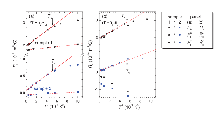
Figure 17: Limiting parameters of the Hall crossover in YbRh₂Si₂. The initial-slope Hall coefficient (open symbols) is plotted against a quadratic temperature scale for two selected samples. Solid lines mark best fits of a quadratic form $R_{\text{H}}(T)=R_{\text{H}}(T=0)+A^{\prime}T^{2}$ to the initial-slope Hall coefficient. The zero-field ($R_{\text{H}}^{0}$) and the high-field ($R_{\text{H}}^{\infty}$) values extracted from fits of eq. (47) to $R_{\text{H}}(B_{2})$ are included in (a). The corresponding values ($\tilde{R}_{\text{H}}^{0}$ and $\tilde{R}_{\text{H}}^{\infty}$) extracted from the single-field Hall results (Fig. 15) are displayed in (b). Arrows mark the Néel temperature. Reproduced with permission from S. Friedemann et al., Journal of Physics: Condensed Matter 23 (2011) 094216 [49]. Copyright (2011) IOP Publishing Ltd.

temperature dependence of the FWHM is displayed in Fig. 18. Like for the crossover field, we find the data sets of the different samples to be in excellent agreement. This emphasizes that the Hall crossover is robust against sample dependencies whereas the background contribution and the absolute values of the Hall coefficient are indeed sample dependent. In addition, the width extracted from the single-field and crossed-field Hall effect measurements and from the analogous crossover in the longitudinal magnetoresistivity match very well. This indicates that we probe the same Fermi surface change with both the Hall and the magnetoresistivity measurement.

As already deduced from the $R_{\text{H}}(B_{2})$ curves, the width of the crossover shrinks as the temperature is reduced. This width reveals a fundamental property of the quantum critical Hall crossover: Taking all these data sets together, the temperature dependent width of the crossover is best described by a proportionality to temperature, see the solid line in Fig. 18. No signature is observed in $\text{FWHM}(T)$ at $T_{\text{N}}$. This is in contrast to $R_{\text{H}}^{0}$ and thus also the height which changes to a quadratic temperature dependence below $T_{\text{N}}$. A tendency towards saturation of $\text{FWHM}(T)$ seems to set in for the crossed-field Hall and longitudinal magnetoresistivity data below 30 mK whereas the single-field Hall-effect data continue the decrease linearly down to the lowest temperature accessed. It is most likely that the crossed-field Hall data are affected by the proximity to the classical phase transition as at these lowest temperatures the Hall crossover significantly interferes with the classical phase transition at $T_{\text{N}}(B)$. This can be seen from the fact that at lowest temperatures the FWHM extends substantially into the ordered phase (cf. horizontal bars in Fig. 16). For the single-field Hall experiment the classical fluctuations should be smaller according to this reasoning. Such a difference may well originate from the different orientation of the tuning field for the two experiments. For the crossed-field Hall experiment with the tuning field in the magnetically easy plane, the magnetization and thus the classical magnetic fluctuations are almost one order of magnitude larger compared to the single-field experiment with the tuning field ($B_{1}$) along the magnetic hard axis. Nevertheless, within the experimental accuracy all data agree with the fit down to the lowest temperatures. Consequently, the FWHM extrapolates to zero in the limit $T\to 0$. Together with the crossover field $B_{0}$ converging to the QCP and the step height remaining finite, the vanishing width suggests that the crossover in the Hall coefficient transforms into a discontinuity at the QCP. This indicates a reconstruction of the Fermi surface.

The single-field and crossed-field Hall experiments reveal a critical crossover in the Hall coefficient which matches in its

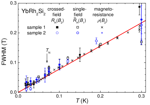
Figure 18: Vanishing width of the Hall crossover in YbRh₂Si₂ after Ref. [53]. The full-width at half-maximum (FWHM) was extracted from the derivative of the fits of eq. (47) to $R_{\text{H}}(B_{2})$ in the crossed-field experiment (closed symbols), to $\tilde{R}_{\text{H}}(B_{1})$ of the single-field Hall data (open symbols) and magnetoresistance (crosses). Inset of Fig. 14 illustrates the definition of FWHM. The values of the single-field experiment were scaled by $1/11$ to account for the magnetic anisotropy. Solid line marks a linear fit to all data sets up to 1 K which intersects the ordinate at the origin within experimental accuracy [49]. Vertical arrow marks the Néel temperature. Reproduced from S. Friedemann et al., Proceedings of the National Academy of Science USA 107 (2010) 14547 [53].

position and width. This is in accordance with the considerations presented in section 4.2. In particular it reflects that according to eq. (38) the single-field Hall results can be decomposed into an orbital contribution and a Zeeman contribution; the former is expected to be identical to the result of the crossed-field Hall experiment. Only the step height appears to be different for the two experiments which should than be associated with the Zeeman term. It remains to be understood in detail how the step height is changed. One possibility is that it may originate from the different field scales involved in the two experiments.

A change of the scattering rates of the two dominating bands crossing the Fermi level [187] can be ruled out as the origin of a jump in the Hall coefficient. The sample dependencies associated with the background contribution are explained incorporating different relative scattering rates of the two bands which arise from minute differences in the composition. The Hall crossover however originates from the quantum criticality. Furthermore, the tuning parameter is varied continuously and tunes the material through a continuous phase transition. A change in the scattering rates at the latter can thus not lead to a discontinuous evolution of the Hall coefficient.

The abrupt change of the Hall coefficient is associated with a Fermi surface collapse which is incompatible with the expectations for an SDW QCP. For an SDW QCP a smooth evolution is expected theoretically [28, 47, 48]. The Fermi surface of a SDW state is reconstructed from that of the paramagnetic state through a band folding. When the SDW order parameter is adiabatically switched off, the folded Fermi surface is smoothly connected to the paramagnetic one. As a result, the Hall coefficient does not show a jump provided the nesting is not perfect [48]. In fact, for the prototypical material of itinerant antiferromagnetism, elemental Chromium, the Hall coefficient seems to evolve smoothly through the QCP. This is seen from studies in which the magnetism is suppressed by hydrostatic pressure or through a combination of Vanadium substitution with pressure [46, 45].

We can rule out that the discontinuity in the Hall effect is related to a breakdown of the low-field limit as it might occur at a field induced SDW QCP. It was pointed out theoretically that for a magnetic-field driven QCP the non-zero critical field can give rise to a small discontinuity in the magnetotransport coefficients even in the case of an SDW QCP [50] (see section 3.4.2). If the energy scale of the vanishing magnetic order becomes smaller than the energy scale associated with the Lorentz force the weak field limit breaks down and this may lead to a non-linearity in magnetotransport. In the Hall coefficient the non-linearities of the conductivities can add to a jump which would be smeared by disorder. Up to date, however, such a jump in $R_{\text{H}}$ at an SDW QCP has not been seen in any other quantum critical system. For the case of YbRh₂Si₂ we exclude this effect by using the crossed-field geometry. This setup allows to apply a vanishingly small Hall field $B_{1}$ while the material is tuned to its QCP via a critical value of the field $B_{2}$. Thus, the energy scale associated with the Lorentz force (arising from $B_{1}$) is negligibly small avoiding the above described breakdown of low-field magnetotransport. In fact, the Hall resistivity remains linear even at the critical value of the tuning field $B_{2}$ as can be seen from Fig. 12. In addition, the signatures due to low-field breakdown are expected to change with residual resistivity. Consequently, the fact that the Hall crossover is observed for two samples with residual resistivities differing by a factor two discards this scenario. Furthermore, with the width and position of the crossover of the single-field experiment being identical to the crossed-field Hall results even the single-field results seem to be unrelated with a breakdown of low-field magnetotransport.

The interpretation of the results from Hall effect measurements in terms of a Kondo breakdown are corroborated by thermal transport [10] and thermodynamic measurements [189]. In particular, the isothermal, linear magnetostriction, $\lambda_{[110]}(B,T)=\partial\ln L/\partial B$ (where $L$ is the length along the [110] direction and $B\!\perp\!c$), has been measured down to temperatures of 20 mK. Interestingly, $\lambda_{[110]}(B,T)$ can be fit by a crossover function analogous to eq. (47) and yields crossover field values $B_{0}^{\lambda}$ in good agreement with those obtained from Hall effect measurements [189]. We note that all the low-temperature measurements on YbRh₂Si₂ so far (including, e.g., magnetostriction, heat capacity and susceptibility) indicated a second order phase transition at $B_{0}$.

Very recently, Hall effect measurements at high magnetic fields have been conducted on YbRh₂Si₂ [190]. Beyond 12 T, the Hall resistivity $\rho_{xy}$ is independent of temperature within the measured range 0.05 K $\leq T\leq$ 2.75 K. This is consistent with a suppression of the Kondo state at these high fields. The Hall coefficient $R_{\rm H}$ exhibits several small features which are in good agreement with changes in the topology of the calculated Fermi surface [191]. The overall increase of $R_{\rm H}$ in the field range between about $6-10$ T may signal the de-renormalization of the Kondo quasiparticles. Most importantly, renormalized band structure calculations [191] indicate the crossing of the Fermi level of one of the spin-split bands at above 10 T which is in line with our Hall results, and a Lifshitz transition at these high fields. We emphasize that—in contrast to these results at high magnetic fields—a Lifshitz transition at small fields $B_{0}$, i.e. close to the QCP, is unlikely, specifically in view of the observed linear increase of the width of the Hall with temperature, FWHM $\propto T$, cf. Fig. 18.

Clearly, it is desirable to support the results of the Hall measurements by other, possibly more direct, probes of the Fermi surface in YbRh₂Si₂, like ARPES or dHvA effect measurements. However, given the low temperatures and small magnetic fields at which consequences of the QCP are expected to be observed a confirmation of the Kondo breakdown scenario by these methods is not suitable at present. Nonetheless, ARPES measurements have been conducted down to about 10 K in zero magnetic field and clearly demonstrated the (dynamical) hybridization between Yb 4$f$ and conduction electrons [192]. Moreover, dHvA effect measurements [193] indicated the presence of a large Fermi surface at about 8 T, i.e., in the Fermi liquid regime of Fig. 1.

5.2 Comparison to other candidates for Kondo breakdown

A continuous evolution of the Fermi surface was identified in CeRu₂Si₂ with the help of Hall effect measurements [194]. In fact, dHvA measurements suggested a localization of $f$ electrons at the metamagnetic quantum phase transition in resemblance to the Kondo breakdown scenario. Hall effect measurements down to below 10 mK, however, revealed a Lifshitz transition as the underlying mechanism: One of the spin-split branches of a Fermi surface sheet shrinks to a point at the metamagnetic critical field giving rise to signatures in both the resistivity and the Hall resistivity. At high temperatures a pronounced maximum is observed in the Hall resistivity which shrinks as the temperature is lowered and transforms to a kink at lowest temperatures. Similar behavior might be present in UPt₃ where only a maximum at elevated temperatures was observed [82]. The small kink as observed in CeRu₂Si₂ would not be resolved in the high-field measurements on UPt₃. Importantly, the slope of the Hall resistivity, equivalent to the differential Hall coefficient, approaches identical values in CeRu₂Si₂ on either side of the transition which basically rules out a Fermi surface reconstruction. This is to be contrasted with the data for YbRh₂Si₂ which show different values of the differential Hall coefficient on either sides of the QCP. In addition, such a Lifshitz transition would lead to drastic changes in the signatures in the Hall effect upon variation of the residual resistivity which is in disagreement with the fact that identical signatures are observed for YbRh₂Si₂ in two samples with residual resistivities differing by a factor of almost 2.

A more complicated Lifshitz transition was recently suggested to explain the measured Hall effect of YbRh₂Si₂ [195]. Here, it is assumed that there is a hitherto unknown ultra-narrow band in the band structure and that one of its Zeeman-split components sinks below (or above) the Fermi energy by the critical field. However, this proposal invokes an unphysically small bandwidth of about 5 $\mu$eV and is unlikely to be relevant to YbRh₂Si₂.

Field induced quantum phase transitions were also studied in two other heavy fermion compounds by means of Hall effect measurements, namely URu₂Si₂ [127] and YbAgGe [196]. In URu₂Si₂ the Hall resistivity nicely tracks the different phases traversed when increasing the magnetic field to beyond 35 T. For each of the phases a proportionality of the Hall resistivity to the magnetic field corresponding to a constant Hall coefficient reflects the different Fermi surface configurations. The transition between these phases occurs abruptly indicating discontinuous phase transitions. In fact, the Hall effect shows no signature at the putative QCP underlying the field-induced phase which surrounds it as a dome. This emphasizes the unique role of YbRh₂Si₂ in which the QCP is not masked by an emergent phase providing the chance to study the Hall effect across the QCP.

In YbAgGe, the differential Hall coefficient shows a crossover like structure similar to that observed in YbRh₂Si₂. Exemplary curves are reproduced in Fig. 19(a). The position of the

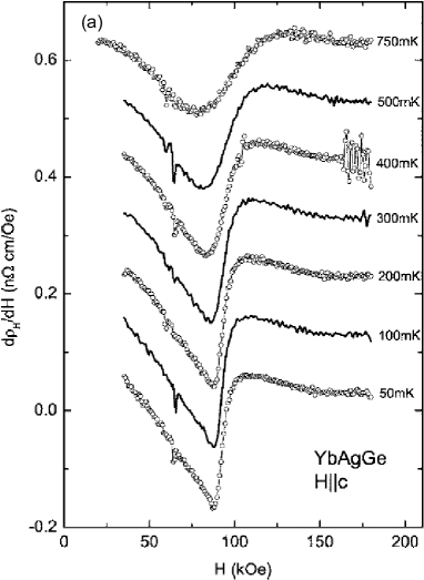
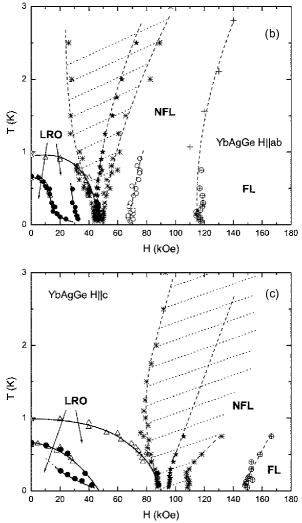
Figure 19: (a) Selected isotherms of the differential Hall coefficient as a function of magnetic field for YbAgGe after Ref. [196]. Magnetic field is oriented parallel to the crystallographic $c$ axis. Except for $T=50$ mK curves are shifted by 0.1 n$\Omega$cm/Oe increments for clarity. Phase diagram for fields perpendicular (b) and parallel (c) to the $c$ axis. LRO denotes the long range magnetically ordered phases. Stars represent the position of the crossover in the differential Hall coefficient and crosses depict the onset and end of the Hall crossover, respectively. They define the width of the Hall crossover which is emphasized by the shaded region. NFL and FL correspond to the non-Fermi-liquid and Fermi-liquid regime as deduced from further features in the differential Hall coefficient. Reprinted figure with permission from S.L. Bud’ko et al., Physical Review B 72, 172413 (2005) [196]. Copyright © (2005) by the American Physical Society.

crossover is tracked in the phase diagram shown in Figs. 19(b) and (c) for two different field orientations. It is apparent that the crossover position is linked to the suppression of long range magnetic order, similar to what was observed in YbRh₂Si₂. However, this seems to be different for the two different orientations. For the field perpendicular to the crystallographic $c$ direction the position of the Hall crossover seems to converge directly to the magnetic instability whereas for fields along the $c$ axis a finite distance appears to persist in the extrapolation to zero temperature. This is in contrast to the results on YbRh₂Si₂ which show identical behavior for both field orientations (cf. Fig. 16). The main difference to YbRh₂Si₂ is, however, that for YbAgGe a finite width of the crossover persists down to zero temperature. This is most prominent for fields along the $c$ axis as can be seen from the finite range of the shaded area at lowest temperatures. Like the position of the crossover also the width is different for different orientations of the magnetic field and can not be scaled by the magnetic anisotropy, in contrast to the findings for YbRh₂Si₂. In summary, these findings represent more complex behavior and, in particular, the finite width favors an SDW scenario for YbAgGe.

Quite recently, the Kondo breakdown scenario has been suggested to be applicable to the cubic heavy fermion compound Ce₃Pd₂₀Si₆ [197]. Although the material crystallizes in a rather complex structure the magnetic Ce ions are arranged on two cubic lattices and in cage-like environments typical for the clathrates [198]. The results of the single-field Hall effect measurements can nicely be analyzed by eq. (47) indicating similarities to the Kondo breakdown in YbRh₂Si₂, cf. Fig. 16. In particular, the crossover in the Hall resistivity also appears to sharpen to a discontinuity in the extrapolation to zero temperature indicating a Fermi surface reconstruction at the critical field of the antiferromagnetic state. In contrast to YbRh₂Si₂, however, the Fermi surface reconstruction does not coincide with the transition into a paramagnetic ground state. Rather, a second ordered phase with higher transition temperature and extending to high magnetic field encloses both the antiferromagnetic phase and the Fermi surface reconstruction. The finite-temperature crossover line associated with the change of the Fermi surface crosses the phase boundary of this second phase at finite temperature in the $B$–$T$ phase diagram of Ce₃Pd₂₀Si₆.

The different behaviors of YbRh₂Si₂ and Ce₃Pd₂₀Si₆ have been discussed in the framework of a global phase diagram in which the degree of quantum fluctuations of the local-moment magnetism frustration is plotted against the normalized Kondo coupling [199, 200, 201]. Both the quantum fluctuations and the Kondo effect weaken magnetic order whereas solely the Kondo coupling is predicted to induce a Fermi-surface reconstruction.

Due to its cubic structure Ce₃Pd₂₀Si₆ is expected to exhibit rather three-dimensional, i.e. small, quantum fluctuations. Therefore, it is naturally settled in the low-frustration regime of the global phase diagram where the Kondo breakdown occurs within the ordered phase, as sketched in Fig. 20. However, it is important to scrutinize this picture further by investigating the NFL behavior associated with the Kondo breakdown and clarifying the nature of the high-temperature ordered phase in Ce₃Pd₂₀Si₆.

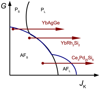
Figure 20: Global phase diagram for heavy-fermion systems. Both magnetic frustration ($G$) and Kondo coupling ($J_{\mathrm{K}}$) suppress the antiferromagnetic (AF) ground state giving way to a paramagnetic phase (P). The Fermi surface reconstruction associated with the breakdown of the Kondo effect marks the crossover from the large Fermi surface (subscript L) which includes the $f$ electrons to the small Fermi surface (subscript S) excluding $f$ electrons. The heavy-fermion compounds YbAgGe, YbRh₂Si₂, and Ce₃Pd₂₀Si₆ are placed according to the observed relation between magnetic order and signatures in the Hall effect. This is justified by structural arguments (see text) giving rise to different levels of quantum frustration. Figure based on Q. Si, Phys. Stat. Solidi B 247, p. 476, 2010 [201]. Copyright (2010) by the WILEY-VCH.

YbRh₂Si₂ has a tetragonal structure and may, therefore, exhibit more two-dimensional fluctuations. This increase in the influence of fluctuation upon lowering the dimensionality would place YbRh₂Si₂ at a somewhat higher frustration level than Ce₃Pd₂₀Si₆. In this regime of the global phase diagram a coincidence of the Kondo breakdown and the magnetic-to-paramagnetic transition is predicted just as observed in YbRh₂Si₂. The separation of the Kondo breakdown and the magnetic transition observed in YbRh₂Si₂ under chemical [202] and hydrostatic [203] pressure indicate that in YbRh₂Si₂ the frustration can be fine-tuned thereby changing its level of frustration and consequently its vertical position in the global phase diagram.

The hexagonal structure of YbAgGe makes this material a promising candidate for further increase of frustration. This would settle YbAgGe in the regime of the global phase diagram where the magnetism is suppressed before the Kondo breakdown is reached. The fact that the signature in the Hall effect for fields parallel to the $c$-direction of YbAgGe is separated from the magnetically ordered phase could be in accordance with this prediction. However, a more detailed analysis of the temperature evolution of the signatures in the Hall effect may possibly allow to scrutinize whether this system undergoes a Fermi surface reconstruction.

5.3 Hall effect and scaling behavior

The proportionality to temperature of the FWHM of the Hall crossover in YbRh₂Si₂, cf. Fig. 18, allows further insight into the nature of the quantum criticality. In order to understand the relevance of this proportionality we have to recall what the Hall coefficient is sensitive to. For the given Fermi liquid ground states on either side of the QCP, the Hall coefficient probes the Fermi surface. $R_{\text{H}}^{0}$ is assigned to the small Fermi surface on the low-field side, and $R_{\text{H}}^{\infty}$ is assigned to the large Fermi surface on the high-field side in agreement with renormalized band structure calculations [187]. At zero temperature, the transition from one Fermi surface to the other is sharp leading to a step in the Hall coefficient. This is in accordance with the experimental observation of a vanishing FWHM. At finite temperature—in the absence of a phase transition—a crossover from one Fermi surface to the other is expected. This is reflected by the crossover in the Hall coefficient. The width of this crossover is determined by the single-electron excitations across the Fermi surface. In the quantum critical regime they obey a linear-in-temperature relaxation rate as a result of the underlying $E/T$ scaling expected for the Kondo-breakdown QCP [53]. These relaxation processes allow a continuous connection of the different Fermi surfaces at finite temperatures. As the Hall crossover appears to mirror the Fermi surface crossover, the linear-in-temperature FWHM hints towards an linear-in-temperature relaxation rate of the single electron states and thus towards an energy over temperature scaling of the electronic excitations [53]. A conventional (3D SDW) QCP, by contrast, is predicted to obey $E/T^{x}$ scaling with $x>1$ which would lead to a super-linear $T$ dependence of both the relaxation rate and the Hall crossover width.

The systematic study of the Hall effect and magnetoresistivity in YbRh₂Si₂ provides currently the best evidence for a Fermi surface reconstruction at a QCP. The discontinuity of the Hall coefficient in the limit of zero temperature reflects this change of the electronic structure. Moreover, the scaling analysis of the Hall crossover width at finite temperatures sheds further light on the unconventional nature of the quantum criticality in YbRh₂Si₂. The proportionality of the FWHM to temperature observed over almost two decades hints towards a linear-in-temperature relaxation rate of the single electron states which itself is linked to $E/T$ scaling of the electronic excitations. Consequently, YbRh₂Si₂ seems to be the first material where both the fundamental signatures of the breakdown of the Kondo effect, a collapse of the Fermi surface and an $E/T$ scaling of the critically fluctuating Fermi surface have been observed. This indicates that the macroscopic scale-invariant fluctuations arise from the microscopic many-body excitations associated with the collapsing Fermi surface. The linkage between microscopics and macroscopics provided by the fundamental $E/T$ scaling is expected to be a keystone to understand the physics of correlated materials. This might apply to a wide class of materials with abnormal finite temperature behavior for which the evolution of the Fermi surface as a function of a control parameter plays a central role like, e.g., in the case of the high-temperature cuprate superconductors.

The crossover in the Hall effect defines a new energy scale called $T^{\star}(B)$ which is confirmed by other transport measurements as well as by thermodynamic measurements [189]. This energy scale vanishing at the QCP is reminiscent of the additional local energy scale proposed in the Kondo breakdown which relates to the break up of the quasiparticles. Interestingly, sufficient changes in the unit cell volume lead to a detachment of the antiferromagnetic QCP from the $T^{\star}(B)$ line. This was realized by isoelectronic substitution on either Rh [202] or Si [204] sites, hydrostatic pressure [203] or a combination of hydrostatic and chemical pressure [205]. For lattice expansion, the $T^{\star}(B)$ line is separated from the magnetic QCP with the intermediate regime featuring non-Fermi-liquid behavior in a finite range of the tuning parameter. It still has to be tested whether the scaling behavior of the Hall crossover persists under lattice changes which might help to understand the nature of the emergent non-Fermi-liquid phase. While the existing experiments have indicated a finite range of chemical pressure in which the two concur [206], this issue deserves further investigation, especially under external pressure. It is also important to examine how this relates to the unconventional critical scaling seen in both the specific heat and Hall effect [207].

6 Hall effect in systems with 115 type of structure

6.1 Influence of magnetic fluctuations on superconductivity

As stated in section 2.5, a remarkable manifestation of quantum many body physics has been the gradual realization that the apparently inimical phenomena of superconductivity and magnetism could be intimately related. At face value, the coexistence of these two diverse electronic ground states seems unlikely, since the prerequisites for these states (itinerant and localized electrons, respectively) appear to be contradictory. Moreover, it was also shown [208] that even small amounts of magnetic impurities were detrimental for the stability of the superconducting condensate in the conventional (BCS) superconductors known at the time. Experimentally, this was supported by early investigations using binary rare earth alloys of the form La${}_{1-x}R_{x}$, ($R$ denotes other members of the Lanthanide series), where the suppression of superconductivity in La appeared to be directly correlated with the 4$f$ spin configuration of the dopant [209]. The effect of impurities has been treated within the theory by Abrikosov and Gor’kov [210]. At a microscopic level, the drastic suppression of superconductivity due to the presence of a magnetic entity can be understood to occur as a result of a “pair-breaking” interaction that arises from the interaction of the magnetic moment ($\mu$) with the spin of the conduction electron (via the Zeeman interaction) or that of its vector potential with the momenta ($\boldsymbol{p}$) of the electrons. The influence of an internal magnetic field generated by a system with (or close to) magnetic order on a BCS superconductor was examined by Berk and Schrieffer [211], who showed that strong (ferro)magnetic exchange would suppress the superconducting ground state. Using the example of Pd, which was known to have an exchange-enhanced spin susceptibility, it was suggested that only a non-superconducting state was feasible for reasonable values of phonon interaction strengths [211].

A relatively simple manner in which magnetism and superconductivity can coexist is by spatial separation, wherein the magnetic sublattice is relatively decoupled from the sea of conduction electrons. This is the case in a variety of systems like the Chevrel phases (of the form $M_{x}$Mo$X_{8}$; where $M$ is a rare earth metal, and $X$ is a chalcogenide) [212], the rhodium borides [213, 214], the ruthenocuprates [215] and the borocarbides [216]. However, the heavy fermion superconductors are distinct in the sense that here magnetism and superconductivity both involve the same set of $f$ electrons, and it was the discovery of heavy fermion superconductivity in CeCu₂Si₂ which unambiguously demonstrated that superconductivity was clearly sustainable in an inherently magnetic environment [2]. Moreover, it was also obvious that these strongly renormalized heavy electrons were a necessary condition for superconductivity, since the homologous LaCu₂Si₂ where the 4$f$ electrons, and consequently, the heavy fermion state were absent did not exhibit a superconducting ground state. Long-range magnetic order is in close vicinity to the superconductivity in CeCu₂Si₂, as is evidenced by the fact that a magnetically ordered state emerges in homogeneous CeCu₂Si₂ samples with very small Cu deficit [217]. This relation between unconventional superconductivity and magnetism is now well recognized, and the heavy fermion systems have turned out to be an interesting testing ground where such emergent behavior is observed. Within the same ThCr₂Si₂ structure, a number of other Ce based systems have now exhibited unconventional superconductivity, thought to be mediated by antiferromagnetic fluctuations. For instance, CeNi₂Ge₂ exhibits ambient pressure superconductivity with a $T_{\rm c}\approx 0.3$ K [218], whereas ambient-pressure magnetic order gives way to pressure-induced superconductivity in CePd₂Si₂ ($T_{\rm N}\approx 10$ K)and CeRh₂Si₂ ($T_{\rm N}\approx 36$ K) [11, 219]. The closely related CeCu₂Ge₂ was also shown to be superconducting at external pressures of the order of 7 GPa [220], though the physics of this system, like CeCu₂Si₂, is complicated by the presence of two superconducting domes [221] that possibly arise from different underlying mechanisms: (i) from a magnetic instability as in the above mentioned systems, and (ii) from charge density fluctuations due to a valence transition in Ce³⁺ [222, 223]. A number of U-based systems also exhibit unconventional superconductivity, notable amongst them being UPt₃ [92] and URu₂Si₂ [93, 94]. In UPt₃ a superconducting condensate was seen to emerge at $T_{\rm c}\approx 0.5$ K from within a magnetically ordered ground state which sets in at around 17.5 K. Though initial analysis of the specific heat was used to speculate on the possibility of ferromagnetic spin fluctuations in this system [224, 225], the antiferromagnetic nature of these correlations was established by the use of neutron scattering measurements [226, 227]. A low temperature superconducting ground state is also observed to emerge from within an ordered magnetic state in the hexagonal UPd₂Al₃ and UNi₂Al₃, with $T_{\rm c}$-values of 2 K and 1.1 K, respectively [95, 228]. A valuable addition to this class of materials has been the Ce$M$In₅ ($M$ = Rh, Ir or Co) family of compounds, discussed in detail in the subsequent sections.

In all the systems mentioned above, superconductivity is observed in the presence (or in the vicinity) of long-range antiferromagnetic order. However, in a small number of heavy fermion systems, the superconducting condensate is known to form in the presence (and through the mediation) of ferromagnetic fluctuations. Needless to say, this places more stringent conditions on the symmetry of the superconducting order parameter, since the spin-singlet state (in which the pairing quasiparticles have opposite spins) is ruled out. In unconventional superconductors in the presence of strong antiferromagnetic fluctuations, stabilization of these spin-singlet Cooper pairs with a non-zero angular momentum is most likely in a $d$-wave state. It is this aspect of heavy fermion superconductivity that binds it with the superconducting cuprates. However, when Cooper pair formation is mediated by ferromagnetic fluctuations, the spin-triplet state is most feasible [229] in which the Cooper pairs have an effective odd angular momentum (analogous to that seen in the superfluid ³He phase). The existence of superconductivity in the vicinity of ferromagnetic order was first demonstrated in UGe₂, where application of external pressures greater than 1 GPa was seen to result in the stabilization of a low-temperature superconducting ground state from within the ferromagnetically ordered state [230]. The orthorhombic URhGe and UCoGe also belong to the same class, with the superconducting condensate being stabilized from within the ferromagnetic ordered state at ambient pressures [231, 232].

6.2 Interplay of magnetism and superconductivity in Ce$M$In₅

The Ce$M$In₅ (where $M$ = Co, Rh or Ir) family of heavy fermion systems have emerged as a focus of intense investigations since the turn of the century. Structurally, these systems can be looked upon as layered variants of the CeIn₃ system, and can be generally described as Ce_n$M_{m}$In_3n+2m, where $n$ layers of CeIn₃ alternate with $m$ layers of $M$In₂ [233]. CeIn₃ is an ambient pressure antiferromagnet, with a transition temperature of 10 K. On the application of pressure, non-Fermi liquid behavior emerges near 2 GPa, where long-range antiferromagnetic order is suppressed to zero temperatures, and superconductivity with a maximum $T_{\rm c}\sim 0.2$ K emerges [11, 234]. Current interest in the Ce$M$In₅ family of systems (equivalent to the $n=m=1$ variants of the general form described above) was sparked off with the observation of pressure-induced superconductivity in CeRhIn₅, with a superconducting transition temperature $T_{\rm c}\approx 2.1$ K at 2.1 GPa [235]. Subsequently, ambient-pressure superconductivity was discovered in the Ir- and Co-based systems [90, 91]. Superconductivity has also been discovered in the $n$ = 2, $m$ = 1 variants, with Ce₂RhIn₈ being superconducting at $T_{\rm c}\sim 1.1$ K at 1.6 GPa [236] and the systems Ce₂CoIn₈ and Ce₂PdIn₈ becoming superconducting at $p=0$ and below $T_{\rm c}\approx 0.4$ K [237] and $T_{\rm c}=0.68$ K [238], respectively. Recently, the first Ce-based (pressure induced) heavy-fermion superconductor of the type $n$ = 1 and $m$ = 2 was discovered: CePt₂In₇ ($T_{\rm c}=2.1$ at $p\approx 3.1$ GPa) [239].

The flurry of attention is primarily due to the intricate interplay between magnetism and superconductivity which this family of heavy fermion metals have demonstrated. For instance, CeCoIn₅ is an ambient-pressure superconductor with a $T_{\rm c}\approx 2.3$ K which is the highest reported value among all Ce based heavy fermion systems to date. Magnetism lies in close proximity to superconductivity in this system, and a magnetic field-induced quantum critical point can be approached by the application of magnetic fields of the order of the superconducting upper critical field ($\mu_{0}H_{\rm c2}\approx$ 5 T) [240]. Several measurements have indicated that the superconducting gap function has line nodes and is most likely to have a $d$-wave symmetry [241]. Closely related is the system CeRhIn₅, which has an ambient pressure antiferromagnetic transition at about 3.8 K. Though the application of pressure suppresses long-range antiferromagnetism, access to the quantum critical point is hindered by the onset of superconductivity [235]. The presence of this magnetic instability has been deduced by specific heat measurements which also point towards the existence of a quantum tetracritical point where four distinct phases (namely, a non-magnetic phase, a superconducting phase, a magnetically ordered phase, and a region within which superconductivity coexists with magnetic order) meet [42]. The existence of this magnetic instability at 2.3 GPa is also reinforced by de Haas-van Alphen measurements indicating an abrupt change in the band structure [41]. The other ambient-pressure superconductor in this series, namely CeIrIn₅, has remained more enigmatic. For instance, unlike its Co counterpart, superconductivity in this system appears to be well separated from the magnetic instability which in the case of CeIrIn₅ is suggested to be metamagnetic in origin [242]. The symmetry of the superconducting gap in CeIrIn₅ has also been a matter of dispute. For instance, measurements of thermal conductivity indicated that the superconducting gap in CeIrIn₅ has a $d_{x^{2}-y^{2}}$ symmetry [243] which is similar to that seen in CeCoIn₅ [244]. This was in contrast to earlier reports which had ascribed the superconducting gap of CeIrIn₅ to be a hybrid one with an $E_{g}$ symmetry [245]. A $d_{x^{2}-y^{2}}$ symmetry of the gap in both these systems would imply that superconductivity in both the superconducting members of the Ce-115 family are likely to be mediated by antiferromagnetic fluctuations in spite of the apparent differences in the position of the superconducting regime with respect to the onset of magnetic order.

The possible difference between superconductivity in the Co and Ir systems is clearly reflected in the phase diagram of solid solutions of Ce$M_{1-x}M^{\prime}_{x}$In₅($M,M^{\prime}$ = Co, Rh, Ir) as shown in Fig. 21, with a possible

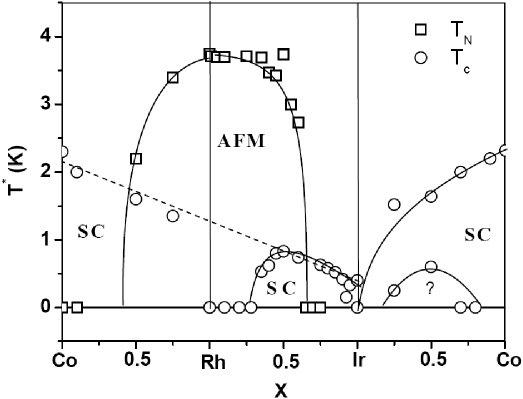
Figure 21: Phase diagram of the system Ce$M_{1-x}M^{\prime}_{x}$In₅ ($M,M^{\prime}$ = Co, Rh, Ir). Reprinted from Physica B 312-313, P.G. Pagliuso et al., p.129 [246]. Copyright ©  (2002) with permission from Elsevier.

superconductor-superconductor critical point at CeRh_0.1Ir_0.9In₅ [246]. This difference is also obvious in doping studies which show that antiferromagnetic order emerges cleanly from within the superconducting ground state in CeCo(In_1-xCd_x)₅, whereas these two ground states appear to be separated from each other in the CeIr(In_1-xCd_x)₅ series of systems [247]. An overview of some of the physical properties of the members of the Ce$M$In₅ family appears in Ref. [248].

6.3 Hall effect measurements on Ce$M$In₅ systems

6.3.1 Scaling relations in Hall effect

Considering the fact that the Ce$M$In₅ systems have been extensively investigated in the recent past, it is not surprising that a substantial amount of Hall data exists in these systems.

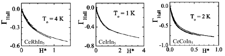
Figure 22: Scaling of the relative change in Hall coefficient ($\Gamma_{\rm Hall}$) as a function of the transformed field parameter $H^{*}$ for the Ce$M$In₅ family. Reprinted figure with permission from M.F. Hundley et al., Physical Review B 70, 035113 (2004) [249]. Copyright © (2004) by the American Physical Society.

These systems have also provided overwhelming evidence for the presence of antiferromagnetic fluctuations, as deduced from Hall effect measurements. Work by Hundley and co-workers [249] in the high-temperature regime (2 K $\leq T\leq$ 325 K) demonstrated that the field-dependent Hall data in the Ce$M$In₅ systems satisfied a scaling relationship that is similar to the one used in analyzing the single-impurity magnetoresistance data. Defining the relative change in the Hall coefficient as

$$\Gamma_{\rm Hall}(H)=\left[R_{\rm H}(H)-R_{\rm H}(H\!\rightarrow\!0)\right]/R_{\rm H}(H\!\rightarrow\!0)\,\,,$$ (48)

it was demonstrated that isotherms of $\Gamma_{\rm Hall}$ plotted as a function of a transformed field parameter $H^{*}$ (defined as $H^{*}=H/(T+T_{0})^{\beta}$, where $H$ is the applied magnetic field and $T_{0}$ and $\beta$ are scaling parameters) could be made to collapse on top of each other. These scaled data plots, which were obtained by fixing $\beta=$ 2 and varying $T_{0}$ are shown in Fig. 22. This scaling analysis yielded $T_{0}=$ 4 K, 1 K and 2 K for the Rh, Ir and Co systems, respectively. These $T_{0}$ values are in reasonable agreement with those estimated for the Kondo temperature from the analysis of specific heat data.

The measured Hall coefficient of the afore-mentioned systems were also expressed as a sum of a skew scattering term and a second one proportional to the Hall coefficient in the non-magnetic La$M$In₅ systems, using a relation:

$$R_{\rm H}^{\rm(Ce)}(H,T)=R_{\rm H}^{skew}(T)+\alpha_{f}(H,T)R_{\rm H}^{\rm(La)}(T)\,\,.$$ (49)

Here, $\alpha_{f}$ was defined as the $f$-electron Hall weighting function. It was shown that $\alpha_{f}$ grows anomalously with the onset of Kondo coherence—the magnitude of which could be suppressed by the application of a large magnetic field—demonstrating the influence of antiferromagnetic fluctuations on the measured Hall response. This line of analysis bears some similarity to the two-fluid Kondo lattice model proposed by Nakatsuji and coworkers [250], who modeled the Kondo lattice system into a component analogous to the Kondo single impurity phase, and one analogous to a coherent heavy fermion phase, with the temperature evolution of the system being determined by a mixing parameter $f(T)$. A key aspect is the fact that whereas the characteristic energy scale in the Kondo single-impurity regime is the single ion Kondo temperature $T_{K}$, in the heavy fermion fluid it is the intersite coupling interaction $T^{*}$. Using La dilution on the Ce site of CeCoIn₅, it was also demonstrated that the condensation of the coherent heavy fermion component is incomplete at the onset of superconductivity. The need for incorporating these effects in combination was of course realized much earlier, for instance in the analysis of neutron scattering data on the system CeCu₆ [251] where a Hamiltonian which accounted for the influence of both the single-impurity Kondo interaction and the RKKY interactions was used. The momentum-dependent magnetic scattering observed in this system was used to infer on the presence of antiferromagnetic correlations which could be quenched by the application of a magnetic field. The presence of these two contributions and a similar behaviour was also established for the material CeRu₂Si₂ [252].

6.3.2 CeCoIn₅

A scaling related to one just described in the previous section was also observed in the low-temperature regime (0.05 K $\leq T\leq$ 5 K) of CeCoIn₅ [253] where it was shown that the Hall coefficient could be scaled into a single generic curve by normalizing their field dependencies by a factor $H_{\rm min}$, as is shown in Fig. 23. Moreover, the $H_{\rm min}$-values which were determined experimentally at low temperatures from a dip in the measured $R_{\rm H}$ (and was thought to represent the inverse of the effective mobility $\mu_{\rm eff}$), could be fit reasonably to a power law, i.e., $H_{\rm min}=a+bT^{c}$. This power law fit as shown in the inset of Fig. 23 yielded $a=4.0\pm 0.7$ T, a result that was taken to be a signature of the fact that the

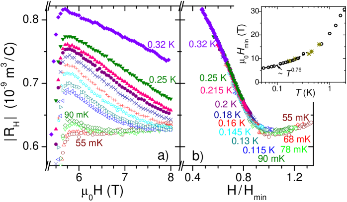
Figure 23: (a) $R_{\rm H}$ as measured in CeCoIn₅. (b) Same data scaled by a normalized field $H/H_{\rm min}$ to obtained maximum overlap. The temperature dependence of $H_{\rm min}$ is depicted in the inset, with the solid line representing a power law fit. Reprinted figure with permission from S. Singh et al. Physical Review Letters 98, p.057001, 2007 [253].

magnetic instability in this system and the superconducting upper critical field lie at separate field values. This conjecture has now been confirmed using measurements of magnetization [254], of the volume thermal expansion [255], of vortex core dissipation [256], of longitudinal magnetoresistance [257] and of field-dependent entropy [258] indicating that the putative QCP lies within the superconducting regime. The critical field for this zero-temperature transition was estimated from the former three types of measurement to be about $(4.1\pm 0.2)$ T which is in excellent agreement to the value deduced from the analysis of the Hall data. This can be seen in the $B$-$T$ phase diagram Fig. 24(a) which was taken from Ref. [255]. Here, data from our Hall measurements, from resistance [259] and magnetoresistance $T(\rho_{\rm max}(B))$ [240] as well as from thermal expansion measurements [255] are compiled.

An interesting manifestation of the possible influence of antiferromagnetic fluctuations on the Hall response was the

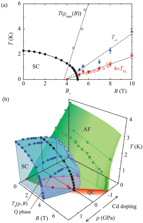
Figure 24: (a) $B$-$T$ phase diagram of CeCoIn₅ at ambient pressure. $T_{cr}$ indicates the change in critical behavior [255] and $T(\rho_{\rm max}(B))$ refers to the position of a maximum in the field-dependent resistance [240]. Fermi liquid behavior is inferred below $T_{\rm FL}$ from thermal-expansion measurements in magnetic field [255] (filled triangle), Hall effect [253] (open squares) and resistivity measurements [259] (open diamonds). A QCP inside the superconducting (SC) phase (located at the field $B_{+}$) is inferred. (b) $p$-$B$-$T$ phase diagram of CeCoIn₅. Shown are results for superconducting transition (black and blue) and Néel temperatures (green) for hydrostatic and negative chemical pressure in CeCoIn_5-xCd_x to demonstrate the relation of antiferromagnetism (AF) and superconductivity. Reprinted figure with permission from S. Zaum et al., Physical Review Letters 106, 087003 (2011) [255]. Copyright © (2011) by the American Physical Society.

observation of a pressure dependent feature in the differential Hall coefficient ($R_{\rm H}^{d}=\partial\rho_{xy}(H,T)/\partial H$) in CeCoIn₅ [253]. Using the same $H_{\rm min}$-values as described in the preceding paragraph, it was shown that $|R_{\rm H}^{d}|$ could be scaled on a curve as shown in Fig. 25. It was suggested that this dip in $|R_{\rm H}^{d}|$ was related to the influence of antiferromagnetic spin fluctuations or a spin-density-wave-driven gap on the Fermi surface. This suggestion was based on the fact that this feature was seen to vanish at applied pressures of the order of 1.2 GPa, which forms the baseline for this curve along with the data at high ($H>1.1H_{\rm min}$) and low ($H<0.5H_{\rm min}$) values of the normalized field. This baseline was thus interpreted to be a reflection of the Fermi liquid regime, and deviations from it were suggested to represent the onset of non Fermi liquid characteristics arising as a consequence of antiferromagnetic fluctuations. The suppression of these magnetic fluctuations by use of pressure in CeCoIn₅ has been documented earlier, and is in reasonable agreement with this scenario [260]. An alternate means of suppressing the incipient antiferromagnetic fluctuations in these systems is by the application of magnetic fields. This was demonstrated by the combined investigation of the electrical and thermal Hall conductivities ($\kappa_{xy}$ and $\sigma_{xy}$, respectively) in the CeCoIn₅ system by Onose and coworkers [261]. Separating out the influence of the electronic contribution ($\kappa_{e}$) and that due to charge-neutral (spin) excitations ($\kappa_{b}$) to the thermal conductivity it was demonstrated that the latter charge neutral term displays an anomalous field dependence. It was suggested that these spin excitations are primarily responsible for the scattering of charge carriers in the non Fermi liquid regime of the phase diagram. Applied magnetic fields rapidly quench these excitations, resulting in a rapid enhancement in the mean free path $\ell$, which in turn is manifested in the form of novel scaling relationships between the magnetoresistance and the thermal and Hall conductivities.

Besides the above mentioned studies which consider the influence of magnetic fluctuations on the scattering of charge carriers,

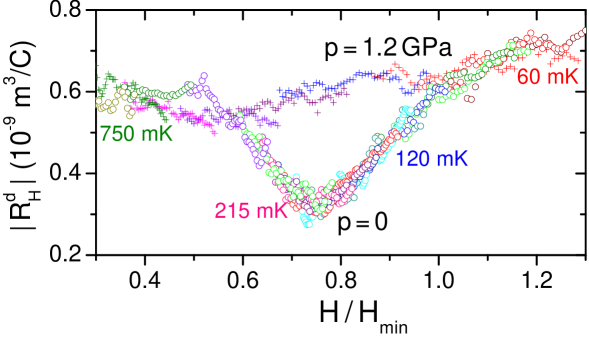
Figure 25: Observation of a pressure dependent feature in the differential Hall conductivity in CeCoIn₅. The baseline represents Landau Fermi liquid behavior, whereas deviations from it arise due to antiferromagnetic fluctuations. Reprinted from [253].

Hall measurements have also been used to infer a possible modification of the Fermi surface, which then manifests itself in the form of anomalous transport properties. This aspect will be dealt with in section 7, in combination with, and in relation to, Hall effect measurements on the high temperature superconducting cuprates.

A number of attempts were made to tailor the balance between magnetism and superconductivity in the CeCoIn₅ system by the use of site-specific dopants. For instance, Sn substitution on the Indium site was seen to suppress the superconducting transition in this system without observable increment in the extent of magnetic fluctuations [262]. A novel perspective in this family of systems was gained by the doping of Cd in the series CeCo(In_1-xCd_x)₅ [247]. Here, magnetism is seen to evolve from within the superconducting ground state as a function of increasing Cd substitution. Preliminary Hall effect measurements on a member of this series CeCo(In_0.925Cd_0.075)₅ revealed an electron dominated Hall response similar to that seen in the parent system [263]. Additional features corresponding to the possible field-induced destabilization of the antiferromagnetic ground state was also observed. Similar observations in the magnetoresistance were then used, in conjunction with neutron diffraction measurements, to chart out the temperature-magnetic field phase diagram in this system [264]. The intertwinned relation of antiferromagnetism and superconductivity is also suggested by the $p$-$B$-$T$ phase diagram, reproduced from [255] in Fig. 24(b). Here, superconducting transition and Néel temperatures are compiled for hydrostatic pressure on CeCoIn₅ and negative chemical pressure in CeCoIn_5-xCd_x.

6.3.3 CeIrIn₅

As mentioned in section 6.2, the magnetic instability is known to be well separated from superconductivity in CeIrIn₅. Moreover, the magnetic instability appears to be metamagnetic in origin [265, 266, 242]; a factor which modulates the temperature-magnetic field phase diagram in this material. For instance, unlike the case of CeCoIn₅, the application of an external magnetic field is seen to suppress, rather than stabilize the Fermi liquid ground state. The metamagnetic nature of the putative quantum phase transition in CeIrIn₅ was also reflected in the scaling analysis of the Hall effect along the lines mentioned in the preceding section where the experimental $R_{H}$ curves within the Kondo coherent regime could be scaled to a generic curve [267]. However, in this case the coefficient yielded a negative value, which was ascribed to the fact that there is no magnetic instability in the immediate vicinity of superconductivity in CeIrIn₅. Analysis of the Hall effect was also used to deduce the presence of a precursor state to superconductivity in this material [268]. This was accomplished by monitoring the field dependence of the Hall angle $\theta_{H}$ in relation to the inverse of the applied field. Deviations from linearity were then used to mark out the existence of a hitherto unidentified state which precedes the formation of a superconducting condensate in this system. The boundary of this precursor state in the temperature-field phase diagram could be scaled onto the boundary of the superconducting regime implying that they could originate from the same underlying phenomena. The existence of this state was in line with prior observations in the related compound CeCoIn₅, where a precursor state to superconductivity was inferred from measurements of the Nernst effect [269] and resistivity under pressure [270].

The anomalous transport properties specifically of CeIrIn₅ are discussed in relation to those of the cuprates in section 7.1.2.

6.3.4 Comparative remarks

As discussed in section 2.5 the competition of RKKY and Kondo interaction may result in quantum critical behavior. Here, a QCP is expected at that value of the experimental control parameter at which the antiferromagnetic order vanishes. However, the excessive entropy related to the QCP is often avoided by the formation of superconductivity [cf. Fig. 26(a)]. Nonetheless, the QCP still lurks around as manifested by non Fermi liquid behavior near the value of the experimental parameter at which the QCP is expected but at temperatures high enough to suppress superconductivity [11, 102].

At temperatures above $\sim$50 K, the Hall coefficient in Ce$M$In₅ with $M$ = Co, Ir, Rh is dominated by skew scattering [249]. Below this temperature, i.e., in a range 2 K $\lesssim T\lesssim$ 50 K, a $T^{2}$ dependence of the cotangent of the Hall angle, $\cot\theta_{H}$, was interpreted to be caused mainly by the complex band structure of these compounds. This was due to the fact that the non-magnetic analogs La$M$In₅ (with $M=$ Co, Ir and Rh) also exhibited a $T^{2}$-dependence of the Hall angle in a similar temperature regime. In systems with complex band structures as has been deduced for the La-115 systems [271], a temperature-dependent Hall response could arise due to different temperature dependencies in the contributing electron and hole bands, see section 3.4.2. In the magnetic Ce$M$In₅ systems, these anomalies would be accentuated due to the addition of strong Kondo and $f$ electron interactions.

At even lower temperatures the results of Hall effect measurements CeCoIn₅ could be used to gauge the crossover from non Fermi liquid to Landau Fermi liquid behavior [253], see section 6.3.2 and Figs. 26(b) and (c). It could be shown that the latter behavior is recovered once the

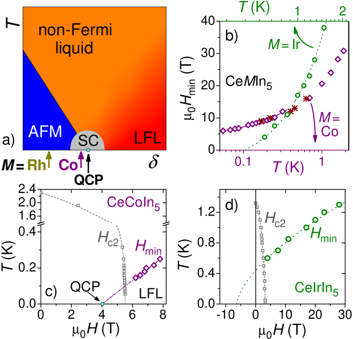
Figure 26: (a) Schematic phase diagram of an archetypical heavy fermion superconductor (SC). The antiferromagnetic (AFM) and Landau Fermi liquid phases as well as the quantum critical point (QCP) are indicated. The positions of Ce$M$In₅ ($M=$ Co, Rh) in their ground states are sketched out. CeIrIn₅ cannot be placed within this schematic due to the first-order nature of its magnetic instability. $\delta$ denotes the experimental control parameter which can be magnetic field or pressure. (b) Comparison of the scaling fields $H_{\rm min}$ for CeCoIn₅ and CeIrIn₅, see Figs. 23, 25. Note the break in the temperature scale. (c) $H\!-\!T$ phase diagram of CeCoIn₅ with the QCP at around 4 T. (d) Phase diagram of CeIrIn₅ without indication of a QCP.

antiferromagnetic spin fluctuations are suppressed either by pressure or magnetic field. As outlined in section 6.3.2, an extrapolation of these results indicated a QCP at around 4 T. Consequently, the quantum critical field is smaller than $H_{\rm c2}$. This important result renders the resulting phase diagram Fig. 26(c) to be in good qualitative agreement with the generic one, Fig. 26(a), if the zero field state of CeCoIn₅ is assumed to be located at a position marked by the arrow in the latter.

Applying the same scaling procedure of the Hall coefficient as outlined for CeCoIn₅ results in a phase diagram for CeIrIn₅ as presented in Fig. 26(d), cf. also section 6.3.3. Clearly, there is no physical meaning of an extrapolation to a negative quantum critical field. But such an extrapolation reveals the close affinity between these two members of the Ce$M$In₅ family: even though there is no indication for a QCP in CeIrIn₅ the zero-field position within the generic phase diagram as marked by the arrow in Fig. 26(a) suggests that the Ir compound nicely fits into this picture. Such a comparison is corroborated by the presence of strong antiferromagnetic fluctuations [272] in both compounds and similarities in superconductivity [244, 243] and Fermi surfaces [273, 248]. This implies that the balance between Kondo and RKKY interaction (section 2.5) is shifted towards the former in case of the Ir compound. This notion is supported by the ratio $T_{\rm RKKY}/T_{\rm K}$ being smaller for Ir ($\approx 7$) if compared to the Co case ($\approx 25$). Within these considerations even CeRhIn₅—which exhibits an antiferromagnetic ground state and superconducts upon application of pressure [42]—fits into the picture ($T_{\rm RKKY}/T_{\rm K}\approx 130$). It should be noted, however, that Fig. 26(a) does not imply that changing the element $M$ in Ce$M$In₅, application of pressure and magnetic field are interchangeable parameters; rather the arrows only indicate the zero-field ground state properties of the respective material.

7 Comparison to Hall effect of other correlated materials

7.1 Copper oxide superconductors and related systems

7.1.1 Cuprates

A discussion of the Hall effect in the heavy fermion metals would not be complete without taking note of how measurements of the Hall effect has influenced the understanding of other strongly correlated electron systems, especially of the high temperature superconducting cuprates. A priori, there appears to be very little in common between these two classes of materials: the heavy fermion metals are inherently metallic systems with a dense array of magnetic ions, whereas the cuprates are doped Mott insulators. However, the emergence of a superconducting condensate in both sets of systems has revealed a number of striking parallels. For instance, the inherently quasi–2D nature of electronic correlations, the proximity of long range antiferromagnetism (or a spin density wave) to superconductivity, a scaling of the observed transition temperatures with the Fermi energy, and the unconventional (possibly $d$ wave) nature of superconductivity in these materials all suggest an underlying similarity in the physics of these materials. A welcome addition to this narrative has been the recent discovery of superconductivity in the oxy-pnictides and related systems.

The discovery of superconductivity in La_2-xBa_xCuO₄ by Bednorz and Müller [274] fuelled an unprecedented interest into many families of the layered cuprates in an attempt to understand the mechanism of superconductivity, as well as to synthesize materials with increasing high superconducting transition temperatures $T_{c}$. Initial Hall effect measurements in these systems were aimed at discerning how these systems differed from conventional metals, and to monitor the sign and evolution of the charge carriers as a function of temperature and doping. Subsequent availability of high-quality single crystalline specimens stirred up the utility of the Hall effect as a probe of the Fermi Surface topology.

In a simple (uncorrelated) metal, where the electron relaxation times are isotropic on all points of the Fermi surface, the Hall coefficient $R_{H}$ would be expected to be independent of temperature. This scenario was thought to be valid for reasonably high temperatures ($T\geq\theta_{D}$, with $\theta_{D}$ being the Debye temperature) where phonons were the dominant scattering mechanism which ensured a reasonably isotropic electron scattering [275]. In practice, $R_{H}$ was seen to be weakly dependent on temperature above a characteristic temperature $T=s\theta_{D}$, where $s$ varies from 0.2 to 0.4 in different metals like Cu, Ag, Cd, and Mg [276, 277, 278]. Below this characteristic temperature, the observed temperature dependence was thought to arise from an increasing anisotropy in an otherwise isotropic Fermi Surface due to residual impurity scattering. Not surprisingly, early Hall measurements on the hole doped cuprates indicated that the scenario in this class of materials was dramatically different. Measurements on La_2-xSr_xCuO₄ [279], YBa₂Cu₃O_7-δ [280, 281, 282, 283] and Tl₂Ca₂Ba₂Cu₃O_x [284] family of systems exhibited a pronounced dependence of the Hall effect on both the temperature as well as the extent of hole doping. Typically, the Hall voltage was seen to be positive, Fig. 27, which at least in the case of La_2-xSr_xCuO₄ was thought to arise from the formation of hole pockets at the corners of the first Brillioun Zone. It was

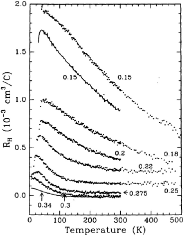
Figure 27: Temperature dependence of the Hall coefficient $R_{H}$ as measured in La_2-xSr_xCuO₄ exemplifying the temperature dependence of the Hall effect in the hole doped cuprates. Reprinted figure with permission from H.Y. Hwang et al., Physical Review Letters 72, 2636 (1994) [285]. Copyright © (1994) by the American Physical Society.

suggested that the area of these pockets increased with increasing hole concentration, which also accounted for the doping dependence of $R_{H}$.

However, experimental signatures like monotonically increasing $R_{H}$ with decreasing temperature in all the measured cuprates could not be understood within the simple picture based on electron-phonon scattering. For instance, in YBa₂Cu₃O₇ the temperature dependence of $R_{H}$ was seen to extend up to 360 K [286]. A simple electron-phonon scattering mechanism as described for simple metals would then warrant an effective $\theta_{D}>900$ K, whereas estimates of $\theta_{D}$ from heat capacity measurements indicated a value which was of the order of 400 K. Measurements on thin films of YBa₂Cu₃O_6+δ indicated that this temperature dependence of the Hall effect continued up to about 700 K [287]. A logical extension was the use of a two-band picture in which the Hall effect from the electrons and the holes partially cancel each other. Thus, the two band Hall effect could be given as (cf. eq. (4) on p. 4)

$$R_{H}=\frac{\mu_{h}-\mu_{e}}{en(\mu_{h}+\mu_{e})}$$ (50)

where $\mu_{h}$ and $\mu_{e}$ refer to the hole and electron mobilities, respectively. In this case, the observed net $R_{H}$ could have a temperature dependence if $\mu_{h}$ and $\mu_{e}$ have different temperature dependencies, and there existed two nearly symmetric bands which fulfil the above equation in a wide range of temperature [288, 289]. However, the fact that this temperature dependence of $R_{H}$ was seen in structurally diverse systems (with different associated Fermi surfaces) like YBa₂Cu₃O₇ and Tl₂Ca₂Ba₂Cu₃O₈, would mean that this rather delicate balance had to exist in all these cuprates in a large part of their phase diagram. The relatively weak pressure dependence of $R_{H}$ as measured in YBa₂Cu₃O₇ [290] would also warrant that $\mu_{h}$ and $\mu_{e}$ have similar pressure dependencies as well. Thus, it was evident that the two band scenario was implausible.

Another potential mechanism for the observed temperature dependence in $R_{H}$ could have been the magnetic skew scattering, described earlier in section 2.3.1. If scattering from the magnetic impurities were relatively independent from each other, the anomalous part of the Hall effect could scale with the (temperature dependent) paramagnetic magnetic susceptibility $\chi$. The validity of this scenario was tested by extending Hall measurements to higher fields, where the Zeeman energy $g\mu_{B}B$ was clearly higher than the thermal energy $k_{B}T$. Here, $g$ refers to the g-factor, $\mu_{B}$ is the Bohr Magneton, $B$ is the applied magnetic field, $k_{B}$ is the Boltzmann constant. At large values of $B$, i.e. $B>k_{B}T/g\mu_{B}$, the paramagnetic susceptibility (and thus the anomalous Hall effect) should saturate, and should be clearly discernible in field sweep experiments. However, it was observed that in La_2-xSr_xCuO₄, the Hall voltage as measured at 52 K remained linear up to fields of the order of 12 T. Measurements on the electron doped system Nd_2-xCe_xCuO₄ indicated that this linear behaviour in the Hall voltage persisted up to 20 T even at temperatures as low as 1.2 K, whereas a typical g-factor value of 2, at $T$ = 2 K should have resulted in a saturation in $\chi$ at moderate fields of the order of 1.5 T.

These anomalous transport properties where the resistivity and the Hall effect had different temperature dependencies could not be accounted for using either the conventional Boltzmann-Bloch models or by incorporating magnetic skew scattering. An additional mystery in the cuprates was the pronounced sensitivity of the Hall effect to in-plane disorder. For instance, the addition of Zn or Co impurities in the CuO₂ planes in YBa₂Cu₃O₇ was seen to result in the suppression of the “Hall slope” defined as $d(1/eR_{H})/dT$ [291]. An important advance in explaining this anomalous behaviour in the cuprates was Anderson’s conjecture that there exist two transport relaxation times in the cuprates which independently influence the Hall effect and the resistivity in these systems [27]. This was in response to the observation that the Hall angle $\theta_{H}$, as defined in eq. (3), has an unambiguous $T^{2}$-dependence in an extended temperature regime, and appeared to be an intrinsic parameter in this class of materials. In normal metals, there is one transport relaxation time $\tau_{\rm tr}$ for electrons on all parts of the Fermi surface, which governs both the resistivity and the Hall effect. Thus the conductivity $\sigma_{xx}$ is proportional to $\tau_{\rm tr}$ and has a $T^{-1}$-dependence (since $\hbar/\tau_{\rm tr}\propto k_{B}T$), whereas the Hall conductivity $\sigma_{xy}$ is proportional to $\tau_{\rm tr}^{2}$, and thus has a $T^{-2}$-dependence. However, using a Luttinger liquid formalism, Anderson suggested that transport in these materials were governed by quasiparticles (spinons and holons) which carry the spin and charge degrees of freedom, and which independently influence the Hall effect and resistivity. According to this picture, the Hall effect is governed by the transverse relaxation rate $\tau_{H}$ which is determined by scattering between spin excitations and has a $T^{-2}$-dependence, whereas $\sigma_{xy}$ is proportional to $\tau_{\rm tr}\cdot t_{H}$, and thus has a $T^{-3}$-dependence.

More importantly, the Hall angle $\theta_{H}$ of eq. (3) relies on $\tau_{H}$ alone and is thus a quantity of fundamental interest. Moreover, it has a $T^{2}$ dependence, and is independent of the impurity scattering which only adds a temperature independent term to both the scattering rates. This, being an easily verifiable prediction, was confirmed on Zn substituted YBa₂Cu₃O₇ [24], as is shown in Fig. 28. This $T^{2}$ dependence of the Hall angle was shown to persist up to temperatures as large as 500 K in oxygen

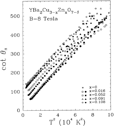
Figure 28: Temperature dependence of the Hall angle as measured in a series of Zn doped YBa₂Cu₃O₇ samples demonstrating the $T^{2}$ dependence of $\theta_{H}$ independent of the impurity concentration. Reprinted figure with permission from T.R. Chien, Z.Z. Wang, and N.P. Ong, Physical Review Letters 67, 2088 (1991) [24]. Copyright © (1991) by the American Physical Society.

reduced samples of the same series by Harris and co-workers [292]. Measurements of the optical conductivity confirmed the non-Drude nature of charge dynamics in thin films of YBa₂Cu₃O₇ and could be qualitatively explained on the basis of the two distinct scattering rates [293]. The $T^{2}$ dependence of the Hall angle is now known to be endemic to many cuprate superconductors and was used extensively to emphasize on the anomalous transport properties of many cuprate families. Prominent examples include the case of Zn, Co, Fe and Pr substituted YBa₂Cu₃O₇ [24, 294, 295, 296], Y, Ni and Zn substituted Bi₂Sr₂CaCu₂O₈ [297], and Fe, Co, Ni, Zn and Ga substituted La_1.85Sr_0.15CuO₄ [298]. An interesting manifestation of the existence of two time scales was the reformulation of the Kohler’s scaling rule in terms of the Hall angle. In conventional metals, the Kohler’s rule mandates that the orbital contribution to magnetoresistance $[\rho_{xx}(H)-\rho_{xx}(0)]/\rho_{xx}(0)$ can be scaled as a function of the term $H/\rho_{xx}(0)$. Harris and co-workers demonstrated that this scaling clearly breaks down in the case of YBa₂Cu₃O₇ and La_2-xSr_xCuO₄ [134]. They also showed that the temperature dependence of the magnetoresistance varies with the square of the Hall angle, which is in line with the scenario of two scattering relaxation rates. A phenomenological transport equation was developed [299, 300] for the cuprates which allowed distinct scattering rates for $\tau_{tr}$ and $\tau_{H}$ as envisaged in the spin-charge separation scenario. This reproduced the violation of Kohler’s rule and made predictions for the thermopower [301] but required the two scattering rates to differ significantly in magnitude which was later shown not to be consistent with optical transport [293].

Besides the spin charge separation scenario, a prime candidate in explaining the anomalous transport properties in the cuprates is the nearly antiferromagnetic Fermi liquid (NAFFL) theory as described in a series of papers by Pines and others [302, 303, 304, 305, 306, 26]. This model relies on an anisotropic reconstruction of the (otherwise isotropic) Fermi surface in the presence of (antiferro-)magnetic spin fluctuations. This is achieved by the formation of “hot” spots and “cold” regions on the Fermi surface, with the hot spots being located at positions in the momentum space where the antiferromagnetic Brillouin Zone intersects the Fermi Surface. All the transport properties would thus be normalized with respect to these (modified) scattering rates. It was suggested [26] that the Hall effect in these NAFFL systems could be broadly classified into three temperature regimes, with $\sigma_{xy}$ varying as $T^{-4}$, $T^{-3}$ and $T^{-2}$ with increasing temperatures. Here, the crossover points between these regimes depend on details of the band structure. In addition to these theories, which rely on the Hall angle being linearly dependent on the scattering rate $\tau_{H}$, the marginal Fermi liquid theory by Varma and co-workers relies on a square scattering response ($\tau^{2}H)$ [160, 307, 308, 309]. Another avenue of interpreting the anomalous magnetotransport measurements within the Fermi liquid formalism is the use of current vertex corrections (CVC) championed by Kontani and co-workers [29]. This refers to the current driven by quasiparticles which propagate though collision events in the Fermi liquid. In a liquid with incipient antiferromagnetic fluctuations, these currents can have a pronounced momentum distribution which then correspondingly modifies the observed magnetotransport properties (see, however, section 3.4.2).

Measurements of the Hall effect, in particular the Hall angle, was also used to speculate on the existence of the pseudogap in some of these cuprates. For instance Abe and co-workers used deviations from the $T^{2}$-behavior in Zn doped YBa₂Cu₃O₇ as a measure of the pseudogap temperature [310]. The direction of change in $\theta_{H}$ at the onset of the pseudogap was used to suggest that the opening of the gap was associated with an enhancement of $\tau_{H}^{-1}$ and a reduction in $\tau_{\rm tr}^{-1}$. A similar deviation of $\theta_{H}$ at the onset of the pseudogap was also reported in the underdoped YBa₂Cu₃O_6.63 system [17]. The temperature scale of the pseudogap was also used to scale the Hall number $n_{H}$ and the Hall angle in films of YBa₂Cu₃O₇ indicating that the pseudogap is an intrinsic energy scale of these systems [311]. Interestingly, a similar line of analysis was used earlier in crystals of La_2-xSr_xCuO₄ where the temperature dependent $R_{H}$ was scaled using an arbitrarily defined temperature scale $T^{*}$, where $T^{*}$ was thought to approximately represent a crossover between a temperature independent to a temperature dependent $R_{H}$ [285, 312].

Fermiology in the Cuprates

The availability of extremely high-quality single-crystal specimens, coupled with sensitive new Hall effect measurements have thrown new light on the nature of the Fermi surface in cuprates. Whereas systems in the overdoped regime of the cuprate phase diagram behave like metals to a reasonable approximation, the underdoped cuprates are characterized by Fermi surfaces made up of discontinuous “Fermi Arcs” as deduced from spectroscopic measurements [313, 314]. An important advance was the observation of quantum oscillations as measured in the Hall resistivity in the underdoped YBa₂Cu₃O_6.5, establishing the existence of a continuous Fermi surface in this class of systems [315]. The Hall response was observed to be negative (unlike the typical positive $R_{H}$ observed in other hole-doped cuprates), and this was attributed at that time to the influence of the vortex liquid phase which persists in this region of the phase diagram. Moreover, the low frequency of the observed Shubnikov–de Haas oscillations indicated the presence of a Fermi surface made up of small pockets. Observation of similar oscillations in the magnetoresistance of YBa₂Cu₄O₈ indicated that the existence of these small pockets were independent of the details of the band structure and could probably be a generic feature of many underdoped cuprate superconductors [316]. Monitoring the sign of the Hall response in the magnetic field regime where these oscillations were observed, LeBoeuf and co-workers concluded that these small pockets were electron like, rather than being hole like [20]. This is surprising considering the hole doped nature of these materials and also because of the fact that the existence of a cylindrical, hole-like Fermi surface in the overdoped cuprates has been documented [317]. This could imply that there exists a Fermi surface reconstruction as a function of hole doping, with a possible zero-temperature instability demarcating these two metallic states. Recently, LeBoeuf and coworkers have reported on a Hall effect investigation on the YBa₂Cu₃O_y system with varying hole doping per planar Cu atom ($p$) from 0.078 to 0.152 [318]. In the $T\!\rightarrow\!0$ limit, the Hall coefficient $R_{H}$ was seen to change from positive to negative, as the doping is reduced below 0.08. This was suggested to arise due to the presence of a Lifshitz transition which modifies the Fermi surface topology. The electron pocket which is observed to persist till the highest investigated doping level ($p=0.152$), was conjectured to arise from an ordered state (like some form of stripe order [319]) which breaks the translational symmetry of the system.

7.1.2 Comparison of cuprates and heavy-fermion systems

The insight gained in investigating the anomalous transport properties of the underdoped

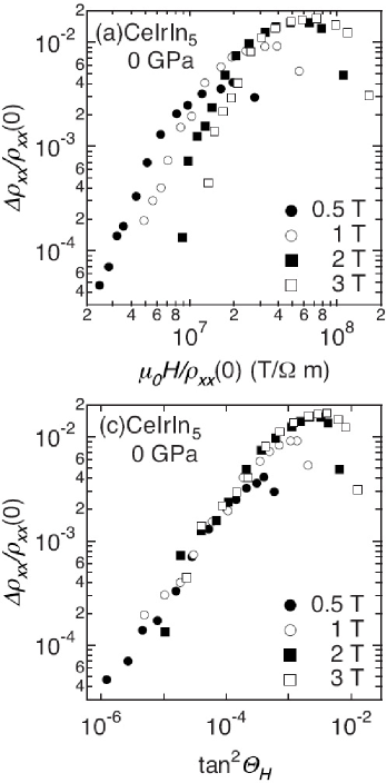
Figure 29: The violation of Kohler’s scaling (upper panel) and its reformulation in terms of the Hall angle (lower panel) as deduced in CeIrIn₅. Reprinted figure with permission from Y. Nakajima et al., Physical Review B 77, 214504 (2008) [320]. Copyright © (2008) by the American Physical Society.

cuprates have found resonance in attempting to understand the nature of pronounced non Fermi liquid characteristics observed in some heavy fermion metals. This is especially so in the case of the magnetotransport in Ce-115 systems, section 6.3, where an acute interplay between superconductivity and quantum magnetism has revealed some striking parallels with that observed in the cuprates. For instance, in both the CeCoIn₅ and CeIrIn₅ systems, a quasi-linear temperature dependence of the resistivity is observed, with this non-Fermi liquid characteristic being driven due to the influence of incipient antiferromagnetic fluctuations [90, 91]. The Hall effect as measured in these systems also shows a pronounced temperature dependence. More importantly, the Hall angle $\theta_{H}$ clearly varies as $T^{2}$ indicating the disparate nature of scattering processes that drive the resistivity and Hall effect in these systems [249, 12, 321, 322, 268, 320]. This is also reinforced by the analysis of the magnetoresistance where the Kohler’s scaling is violated, and the scaling procedure is only seen to work when equated in terms of the Hall angle as is shown in Fig. 29.

In CeIrIn₅, an additional anomaly in the form of a breakdown of the modified Kohler’s scaling is observed very close to the onset of superconductivity. However, this is due to the influence of a precursor state to superconductivity in this system, which influences the resistive and Hall scattering rates in disparate fashions [268]. The existence of this precursor state was inferred from the field dependence of the Hall angle, and was thought to represent an anisotropic reconstruction of the Fermi surface prior to the formation of the superconducting condensate. In line with prior investigations in the cuprates where the energy scale associated with the pseudogap was used to scale the resistivity and the Hall effect [311], a model-independent single parameter scaling of the Hall angle was observed in CeIrIn₅ implying that the precursor state represented an intrinsic energy scale of the system [18]. Interestingly, neither the resistivity nor the Hall effect could be individually scaled using the precursor state, implying that the onset of this precursor state selectively influences the Hall channel alone. This is in consonance with that observed in the underdoped YBa₂Cu₃O_6.63 where the opening of the pseudogap was seen to significantly reduce the Hall response leaving the resistivity relatively unaffected [17]. Unlike the systems CeCoIn₅ and CeIrIn₅, which lie on the paramagnetic side of the putative Quantum critical point, CeRhIn₅ orders antiferromagnetically at ambient pressures. Application of external pressure shifts this system towards a superconducting ground state, and in this regime the pronounced non-Fermi liquid

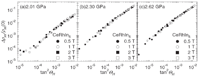
Figure 30: Modified Kohler’s plots equating the magnetoresistance with the Hall angle as measured in CeRhIn₅ at pressures above 2 GPa. Reprinted with permission from Y. Nakajima et al., Journal of the Physical Society of Japan 76 (2007) 024703 [12]. Copyright (2007) by the Physical Society of Japan.

properties enumerated above are retrieved. Fig. 30 shows the modified Kohler’s plot as deduced in CeRhIn₅ for a range of pressures above 2 GPa where superconductivity is observed.

Though this similarity between the heavy fermion metals and the superconducting cuprates is surprising, this common ground is possibly brought about by the ingredient which influences the electronic properties of both these systems, viz., the presence of antiferromagnetic fluctuations. In magnetotransport, this is reflected in the form described above, with the Hall and resistivity being dictated by two different scattering rates. Unfortunately, an analysis of this nature mandates the simultaneous measurements of the Hall effect and the resistivity which at least in the case of heavy fermion systems has been scarce. However, it is interesting to note that for all the systems where such measurements have been reported—namely, the members of the Ce-115 family and YbRh₂Si₂ [176]—a $T^{2}$-dependence of the Hall angle has been found along with a quasi-linear temperature dependence of resistivity. The fact that this behaviour is observed in spite of the wide span of low temperature electronic ground states observed in these materials implies that the scenario of two scattering times could be a feature of many heavy fermion systems.

7.1.3 Hall effect in the oxy-pnictides and related systems

A valuable addition to the existing assemblage of strongly correlated electron systems was the discovery of high temperature superconductivity in an iron based system by Kamihara and co workers [323]. The consequent flurry of activity (for a review see, e.g., [324]) has revealed that emergence of superconductivity in the proximity to a magnetic instability could be a factor which binds these systems with the heavy fermion systems and the high temperature cuprate superconductors in spite of the different band structures of these systems. Though analysis of Hall effect measurements on these systems have not been extensive till date, there is enough indication at the time of writing this review to indicate the anomalous nature of the magnetotransport in this class of materials. For instance, Cheng and co-workers reported on the Hall effect and magnetoresistance in single crystals of NdFeAsO_1-xF_x and observed a pronounced temperature dependence of the Hall effect [325]. Moreover, analysis of magnetoresistance revealed a breakdown of Kohler’s scaling in this system. The temperature evolution and, more importantly, the sign change of $R_{H}$ in Ba(Fe_1-xCo_x)₂As₂ was used to conjecture on the nature of the electron-hole asymmetry in this system [326]. Using a two-band Fermi liquid model it was inferred that the electrons and holes in this multiband system have disparate scattering rates. Similar inferences were also drawn by Rullier-Albenque and coworkers [327]. The use of the two-band Fermi liquid formalism in both these works meant, however, that the utility of non-Fermi liquid models were not explicitly considered.

An interesting pointer in this regard is a recent use of the Hall effect in monitoring the doping-induced evolution from a Fermi liquid to non-Fermi liquid regime in BaFe₂(As_1-xP_x)₂ [328, 329]. In this series of samples, increasing P substitution suppressed the spin-density-wave transition near the

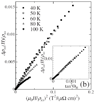
Figure 31: Violation of conventional Kohler’s scaling in BaFe₂(As_0.67P_0.33)₂. Inset shows the modified Kohler’s plot with the magnetoresistance equated in terms with the Hall angle. Reprinted figure with permission from S. Kasahara et al., Physical Review B 81, 184519 (2010) [329]. Copyright © (2010) by the American Physical Society.

end point of which a superconducting regime was uncovered. For the optimally doped system (with $x=0.33$), pronounced non-Fermi liquid characteristics like a linear $T$-dependence of the resistivity and a violation of Kohler’s scaling were observed. Moreover, a modified Kohler’s scaling which again relates the magnetoresistance with the Hall angle was observed, as shown in Fig. 31. This observation indicates that the anomalous transport properties in at least some of these multiband systems could mirror those observed in the cuprates and the heavy fermion systems.

7.2 Other systems of related interest

The possibility of the Hall effect and the magnetoresistance having different scattering rates has also been discussed in a few other strongly correlated systems. For instance, in the prototypical Mott Hubbard system V_2-yO₃ a pronounced temperature dependence of $R_{H}$ was observed [330]. Moreover, the temperature dependence of the Hall effect and the magnetoresistance in the paramagnetic regime was different; with the Hall angle $\theta_{H}$ and the resistivity $\rho_{xx}$ varying as $T^{2}$ and $T^{1.5}$, respectively. This was ascribed to the possibility of a zero temperature metal insulator transition, which is driven by hole doping in the 3$d$ band as a consequence of increasing vanadium deficiency. Another celebrated example is metallic chromium in which the long-range magnetic order can be driven to absolute zero by alloying with small amounts of vanadium, with the putative QCP being approached at critical concentrations of about $x=0.035$ in the Cr_1-xV_x system. Magnetotransport in specimens of this concentration revealed a temperature dependent $R_{H}$ in conjunction with a $T^{3}$-dependence of $\rho_{xx}$ and a $T^{2}$-dependence of the Hall angle $\theta_{H}$ [44].

The organics have emerged as in interesting playground in which strong electronic correlations drive a host of novel electronic ground states in close proximity to each other in phase space. Though analysis of the Hall effect in conjunction with the magnetoresistance has been relatively scarce in this class of materials, a few examples do exist in current literature. For instance, measurements of magnetotransport in the superconducting salt $\kappa$-(BEDT-TTF)₂Cu[N(CN)₂]Cl in the pressure range between 4 to 10 kbar reveal a $T^{2}$ dependence of the Hall angle $\theta_{H}$ whereas the resistivity appears to be sub-linear [331]. Similar behavior was also observed in the system $\Theta$-(DIETS)₂[Au(CN)₄] where measurements of the Hall effect and magnetoresistance under pressures between 5 to 20 kbar along the $c$-axis revealed a linear $T$-dependence of the resistivity, along with a $T^{2}$-dependence of $\theta_{H}$ over a reasonable temperature span [332]. Considering the fact that these anomalous transport properties appear to transcend material classes and is observed in systems as diverse as the cuprates, the heavy fermions, the organics, and other correlated metals, we suggest that this disparity between the Hall effect and the magnetoresistance could be a generic feature of many correlated systems in the presence of strong (antiferro-)magnetic fluctuations.

7.3 Colossal magnetoresistive manganites

A recently highly active field of research in condensed matter physics is concerned with the manganites, $R$MnO₃ with $R$ being a rare earth, and their doped variants, $R_{1-x}$$A_{x}$MnO₃ where $A$ denotes a divalent or tetravalent cation. Also in this class of materials the correlations between the electrons play a crucial role [333]. These correlations involve structural, charge, orbital as well as spin degrees of freedom leading to a vast variety of different types of order that may result in competition, or even coexistence, of different phases. The balance between these phases can be subtle such that small changes of a tuning parameter (again, e.g., chemical composition or magnetic field) prompt a significant response of the material’s properties. Typical examples here are the metal-insulator transition (MIT, at a temperature $T_{\rm C}$) and the so-called colossal magnetoresistance (CMR, an unusually strong change of resistance with applied magnetic field) [334]. Even though the CMR effect with its potential technological applications [335] has originally drawn the research interest to the manganites, their rich phase diagrams due to the above-mentioned four degrees of freedom which gives rise to the possibility for intrinsic inhomogeneity appears to be of more contemporary interest [336]. The phase coexistence with inhomogeneous electronic or/and magnetic material properties makes the manganites also prime candidates for local probes like scanning tunneling microscopy and spectroscopy (STM/S) or magnetic force microscopy (MFM).

Although the manganites seem to be quite different from the heavy-fermion metals there are a number of similarities beyond the mere statement of both being strongly correlated electron systems [337]. The above-mentioned Kondo effect was originally developed for single magnetic impurities in metals [85]. In the heavy fermion metals, however, the magnetic ions are periodically arranged on the lattice and may actually interact. Therefore, a variant of the Kondo model, often referred to as the “Kondo lattice model” [338, 339], needs to be considered in which the (often antiferro-) magnetic interaction between localized moments and itinerant electrons at each relevant lattice site is taken into account. On the other hand, the famous double exchange [340] mediates the ferromagnetic coupling between Mn³⁺ and Mn⁴⁺ ions through two simultaneous hopping events of the $e_{g}$ conduction electrons via the intermediate O^2- ion in the manganites. Consequently, the double exchange model can be considered as similar to the Kondo lattice model just with ferromagnetic coupling of local moments and conduction electrons [341]. The combination of spin—resulting from localized electrons—and charge—carried by conducting electrons—degrees of freedom is also at the base of spintronics [342], and the dilute magnetic semiconductors [343] bear some resemblance to the Kondo impurity problem. Moreover, the phenomenon of phase separation (in the sense of locally inhomogeneous electronic or/and magnetic properties) is certainly not only discussed for magnetic oxides (see e.g. [344]) but was applied early on to doped Eu chalcogenides [345, 346], to the thorium phosphide-type structures [347] and to EuB₆ [348]. Also, in its “stripe” version it has been considered for cuprate superconductors [349, 350] and may even be at play within the coexistence range of antiferromagnetism and superconductivity in CeCu₂Si₂ [351].

Hall effect measurements in the manganites were used to infer the Fermi surface of these materials [352, 353]. LaMnO₃ is an insulating A-type antiferromagnet whose magnetic properties are brought about by superexchange. The gap in the density of states (DOS) right at $E_{F}$ is nicely reproduced by band structure calculations within the local density approximation (LDA), e.g. in Ref. [354]. Considering a simplified picture of a rigid band structure it is obvious that either removing or adding electrons, i.e. lowering or raising $E_{F}$ with respect to the bands, may result in a conducting material at low temperature. The usual hole doping (e.g. by Ca or Sr) results in a corresponding mixture of Mn⁴⁺ and Mn³⁺ whereas a less well-known electron doping (e.g. by Ce) gives rise to Mn²⁺ and Mn³⁺. Both types of mixed valencies allow (within a certain doping range) for Zener double exchange with a ferromagnetic metallic ground state of the material. The metallic state prevails up to the ferromagnetic transition at $T_{\rm C}$ where the mobility of the electrons decreases due to spin disorder, and the carriers are localized via the formation of Jahn-Teller polarons. Hence, the polaronic insulating state results from the local lattice deformation around Mn³⁺, and these materials can be considered as polaronic semiconductors above $T_{\rm C}$ [355, 356].

Hall measurements on the manganites are notoriously difficult because of often large contributions from the (negative) anomalous Hall effect and the magnetoresistance [333]. Nonetheless, some results of Hall measurements in the more common hole doped manganites were reported, see e.g. [357] for an excellent overview. For example, charge carrier densities of $n\approx 10^{29}$ m^-3 for La_0.65(PbCa)_0.35MnO₃ at $T=5$ K were obtained [358] as expected for a typical metal. At higher temperatures, sign reversals of $R_{\rm H}$ were observed [359, 360] which could be a result of different bands contributing to the Hall response, see below. In films there could be additional localization effects of charge carriers due to strain or disorder [361].

Another issue becomes specifically obvious if nominally electron doped manganites are considered: the resulting valency of the Mn ions does not only depend upon the $A$-site doping level $x$ but also on the oxygen stoichiometry $\delta^{\prime}$ where La_1-xA_xMnO${}_{3+\delta^{\prime}}$ [362]. Electron doping in films La_0.7Ce_0.3MnO₃ grown by pulsed laser deposition (PLD) at low oxygen partial pressure ($\lesssim 10$ Pa) was evidenced not only by x-ray absorption spectroscopy [363, 364] but was discernible also in Hall effect measurements [365]. However, with increasing oxygen content the material is driven more and more into hole doping [366]. This is sketched in Fig. 32: While oxygen excess (going upward in Fig. 32) is of no harmful consequence to the nominally hole (e.g. Ca) doped manganites it can easily outweigh or even overcome the intended electron doping through Ce substitution in La_1-xCe_xMnO${}_{3+\delta^{\prime}}$ resulting in an effective Mn³⁺/Mn⁴⁺ mixture [367, 368]. In addition,

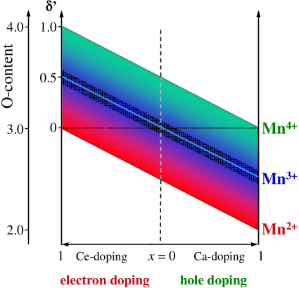
Figure 32: Illustration of the Mn valence resulting from both, the doping on the La site (abscissa) as well as the oxygen content (ordinate) in La_1-xCa_xMnO${}_{3+\delta^{\prime}}$ or La_1-xCe_xMnO${}_{3+\delta^{\prime}}$. The Mn valence is color-coded in red, blue and green presenting Mn²⁺, Mn³⁺ and Mn⁴⁺, respectively. Sufficiently high O-excess can easily outweigh an electron doping intended by Ce substitution of La, and may even result in an unwanted Mn³⁺/Mn⁴⁺ mixture.

unwanted phases (e.g. CeO₂) are very likely to be found in the electron-doped manganites [368, 366]. The formation of additional phases is certainly also supported by the small tolerance factor ($t\approx 0.91$ for La_0.7Ce_0.3MnO₃) resulting from the small size of the tetravalent ions [369, 370]. The small $t$ may also explain the fact that mostly thin films of La_0.7Ce_0.3MnO₃ or other [371, 372] electron doped manganites could be synthesized; with the exception of La_0.9Te_0.1MnO₃ for which electron doping in bulk samples was shown by Hall effect measurements [373]. All these difficulties might easily explain the contradicting results found in the literature as much as they render the electron doped manganites less attractive for further applications.

As already discussed in section 2.2 an anomalous contribution to the Hall effect is expected in magnetic materials, cf. eq. (2). For several manganites it was found that the AHE is negligible at low temperature $T\ll T_{\rm C}$ but contributes significantly to $\varrho_{xy}$ as $T$ is raised towards $T_{\rm C}$ [374, 375, 357, 365, 376, 377]. For La_2/3Sr_1/3MnO₃ and within the metallic phase a linear relationship between $R_{\rm S}(T)$ and $\varrho_{xx}(T)$ as well as the temperature driven change of magnetization, $M(0)-M(T)$, was reported [378]. A similar relation, $R_{\rm S}\propto\varrho_{xx}^{\alpha}$, holds in La_1-xCa_xMnO₃ with $\alpha=1.38$ for $x=0.3$ and $\alpha=0.6$ for $x=0.67$ where electron-type carriers were observed [353]. Below $T_{\rm C}$ the metallic manganites behave as bad metals with the transport being dominated by holes of low mobility [333, 357, 377]. For comparison we wish to add that well above $T_{\rm C}$ the bandwidth of the $e_{g}$ electrons is narrowed by the Jahn-Teller distortion along with strong electron-phonon interactions which causes the formation of small polarons [333, 379] whereas manganites in the insulating regime are governed by variable-range hopping.

Certainly the most interesting temperature regime is the one around the MIT. An early Hall effect study [374] on La_1-xCa_xMnO₃ thin films focusing on this temperature range again reported $R_{\rm S}\propto\varrho_{xx}$ as well as the Hall angle (see eq. (3)) $\tan\theta_{\rm H}\sim M$ for $T>T_{\rm C}$. It was pointed out that the large value of $R_{\rm S}$ in the hopping regime of the manganites is different from the anomalous Hall effect in typical ferromagnetic metals (cf. sections 2.2 and 2.3). While hopping the electrons acquire a phase that reflects their induced alignment to the core spins and is consequently governed by the magnetization [374]. Based on such ideas a model for the AHE was developed [375, 357] that takes into account the quantal phase due to strong Hund’s-rule coupling and the spin-orbit interactions.

We note that an additional (positive) contribution to the AHE is observed in polycrystalline thin films due to grain boundaries [380].

In layered manganites La_2-xSr_1+xMn₂O₇ an additional contribution to the AHE is observed possibly related to the intrinsic inhomogeneity resulting from the spin glass state [381, 382]. In contrast to the manganites, the pyrochlore Tl₂Mn₂O₇ exhibits a negligible AHE and its CMR near $T_{\rm C}$ is governed by a change in charge carrier density [383]. Similarly, the CMR observed in Eu_0.6Ca_0.4B₆ appears to be related to a crossover from hole- to electron-dominated transport [384].

8 Summary

The quest of shedding light on such highly complex materials as the strongly correlated electron systems calls for a comprehensive study and sophisticated experimental approaches. Amongst the plethora of laboratory based tools routinely employed in the investigation of strongly correlated electron systems, Hall effect measurements have proven to be an exemplary one. With other measurement techniques often not feasible in the temperature and field range of interest for heavy fermion compounds, Hall effect measurements can provide insight into the evolution of their renomalized Fermi surfaces, even across a quantum critical point. As such, it remains unparalleled in tackling some of the outstanding problems at the frontiers of current condensed matter physics. Though demonstrated in the case of a prototypical heavy fermion system, YbRh₂Si₂ in section 5.1, the inferences drawn therein are crucial for understanding the physics of systems like heavy fermion superconductors (in section 6 we focused on those with 115-type of structure) or even the cuprates, in which magnetism and superconductivity appear to be inexorably intertwined. The possibility that a similar Fermi surface reconstruction occurs at the crossover from the overdoped to the underdoped regime in the high temperature superconducting cuprates continues to be at the focus of extensive investigations. A related development pertains to the possibility of two scattering times in the heavy fermion systems as deduced from recent Hall measurements in some Ce-based heavy fermions—very much in similarity to that observed earlier in the cuprates. The recently discovered Fe-based superconductors also appear to share some of these intriguing properties. Considering current issues related to sample purity in these systems, it is not unrealistic to predict that they would continue to be extensively investigated for several years to come.

In this review we focused on the investigation of Fermi surface effects in heavy fermion metals. Consequently, we concentrated on the normal contribution to the Hall effect, leaving the anomalous Hall effect aside, even though it also may yield valuable information [67]. Fortunately in this context, the anomalous contribution is often negligibly small for heavy fermion compounds at low temperatures, see section 2.6. Our material basis also implies that the active research areas of the quantized Hall effect [385], its fractional counterpart [386] as well as the related, topical spin Hall effect [387] and topological phases [388] are not touched upon.

Hall effect measurements probe the electronic states directly at the Fermi energy $E_{\rm F}$. As a major advantage, such measurements can be conducted over a wide parameter space, e.g. in temperature, magnetic field (including pulsed fields) or pressure, making this an invaluable probe. Moreover, the results of Hall measurements can be compared to theoretical predictions, or could serve as input for theoretical considerations. Here, Hall effect measurements on YbRh₂Si₂ constitute a good example, as outlined in section 5.1. The theoretical prediction and interpretation have taken advantage of the simplification the zero-temperature limit brings about to the evolution of the Hall coefficient across a quantum critical point. At the same time, we have emphasized that for quantitative understandings as well as for the description of the Hall coefficient at finite temperatures, it is often important to incorporate the complexities in the band structure, such as the multiplicity of the bands, or the various interaction effects on the electronic excitations near the Fermi surfaces. Experimentally, it can be challenging to get the samples into the thin, plate-like shape shown in Fig. 3. As many of these materials are good metals the thickness $d$ often needs to be as small as a few tens of micrometers to give reasonably measurable Hall voltages of several ten nV. In providing detailed information about the measurement technique (section 4) as well as some basic theoretical background (section 3) we wish to inspire more research within the exciting field of heavy fermion physics and, hopefully, beyond.

9 Appendix

The following list provides references in which results of Hall effect measurements are presented for numerous heavy fermion and related materials. It is meant to serve as a guide and is by no means exhaustive.
          Compound Reference CeCu₂Si₂ [113, 389, 390, 391, 392] (Ce_1-xLa_x)Cu₂Si₂ [391] CeRu₂Si₂ [115, 194] CeRh₂Si₂ [39] CeNi₂Ge₂ [393] CeNiGe₃ [394] CeAl₂ [395, 396, 392] Ce(Al_2-xCo_x) [397] CeSn₃ [392]

Compound	Reference
CePtSi	[119]
CeCu6	[114, 121, 389, 398, 399]
(Ce1-xLax)Cu6	[399]
CeB6	[400]
(Ce1-xLax)B6	[401, 400]
CePd3	[113, 392]
(Ce1-xYx)Pd3	[120]
Ce(Pd0.88Ag0.12)3	[113, 392]
CeBe13	[113, 392]
CeRh3	[392]
CeIn3	[402]
CeAl3	[115, 403]
(Ce1-xLax)Al3	[403]
CeCoIn5	[12, 249, 253, 261, 321, 322]
CeCo(In1-xCdx)5	[263]
CeRhIn5	[12, 249, 321, 322]
CeIrIn5	[249, 267, 268, 320]
Ce3Pd20Si6	[197]
Ce2RhIn8	[404]
Ce2IrIn8	[404]
Ce2CoIn8	[405]
Ce2PdIn8	[406]
CePt2In7	[407]
YbRh2Si2	[49, 53, 176, 186, 190]
YbCuAl	[113, 408]
YbCu2Al2	[113, 408]
YbNi2B2C	[409]
YbAgCu4	[410]
YbInAu2	[113, 408]
YbAgGe	[196]
YbPd	[408]
YbAl2	[408]
YbAl3	[408, 411]
U2Zn17	[122]
URu2Si2	[124, 127, 128]
U(Ru0.96Rh0.04)2Si2	[412]
UPt3	[82, 115]
U2PtC2	[413]
UAl2	[115]
UGe2	[414]
UBe13	[114, 413, 415]
UPd2Al3	[416]
NpPd5Al2	[417, 418]

References

- [1] N. Grewe and F. Steglich, Heavy Fermion metals, in Handbook on the Physics and Chemistry of Rare Earths, K.A. Gschneidner, Jr. and L. Eyring, eds., Elsevier Amsterdam, 1991, p. 343.
- [2] F. Steglich, J. Aarts, C.D. Bredl, W. Lieke, D. Meschede, W. Franz, and H. Schäfer, Phys. Rev. Lett. 43 (1979), p. 1892.
- [3] H.R. Ott, H. Rudigier, Z. Fisk, and J.L. Smith, Phys. Rev. Lett. 50 (1983), p. 1595.
- [4] J.A. Hertz, Phys. Rev. B 14 (1976), p. 1165.
- [5] H. von Löhneysen, A. Rosch, M. Vojta, and P. Wölfle, Rev. Mod. Phys. 794 (2007), p. 1015.
- [6] P. Gegenwart, Q. Si, and F. Steglich, Nature Phys. 4 (2008), p. 186.
- [7] J. Custers, P. Gegenwart, H. Wilhelm, K. Neumaier, Y. Tokiwa, O. Trovarelli, C. Geibel, F. Steglich, C. Pépin, and P. Coleman, Nature 424 (2003), p. 524.
- [8] H. von Löhneysen, T. Pietrus, G. Portisch, H.G. Schlager, A. Schröder, M. Sieck, and T. Trappmann, Phys. Rev. Lett. 72 (1994), p. 3262.
- [9] M.A. Tanatar, J. Paglione, C. Petrovic, and L. Taillefer, Science 316 (2007), p. 1320.
- [10] H. Pfau et al., Nature 484 (2012), p. 493.
- [11] N.D. Mathur, F.M. Grosche, S.R. Julian, I.R. Walker, D.M. Freye, R.K.W. Haselwimmer, and G.G. Lonzarich, Nature 394 (1998), p. 39.
- [12] Y. Nakajima et al., J. Phys. Soc. Jpn. 76 (2007), p. 024703.
- [13] L. Taillefer and G.G. Lonzarich, Phys. Rev. Lett. 60 (1988), p. 1570.
- [14] C.M. Hurd The Hall effect in Metals and Alloys, Plenum Press, New York, 1972.
- [15] J. Smit, Physica 21 (1955), p. 877 ibid 24, 397 (1958).
- [16] A. Fert and P.M. Levy, Phys. Rev. B 36 (1987), p. 1907.
- [17] Z.A. Xu, Y. Zhang, and N.P. Ong arXiv:cond-mat/9903123.
- [18] S. Nair, M. Nicklas, F. Steglich, J.L. Sarro, J.D. Thompson, A.J. Schofield, and S. Wirth, Phys. Rev. B 79 (2009), p. 094501.
- [19] F.F. Balakirev, J.B. Betts, A. Migliori, S. Ono, Y. Ando, and G.S. Boebinger, Nature 424 (2003), p. 912.
- [20] D. LeBoeuf et al., Nature 450 (2007), p. 533.
- [21] F.F. Balakirev, J.B. Betts, A. Migliori, I. Tsukada, Y. Ando, and G.S. Boebinger, Phys. Rev. Lett. 102 (2009), p. 017004.
- [22] R.S. Allgaier and R. Perl, Phys. Rev. B 2 (1970), p. 877.
- [23] N.C. Banik and A.W. Overhauser, Phys. Rev. B 18 (1978), p. 1521.
- [24] T.R. Chien, Z.Z. Wang, and N.P. Ong, Phys. Rev. Lett. 67 (1991), p. 2088.
- [25] N.P. Ong, Phys. Rev. B 43 (1991), p. 193.
- [26] B.P. Stojkovic and D. Pines, Phys. Rev. B 55 (1997), p. 8576.
- [27] P.W. Anderson, Phys. Rev. Lett. 67 (1991), p. 2992.
- [28] P. Coleman, C. Pépin, Q. Si, and R. Ramazashvili, J. Phys.: Condens. Matter 13 (2001), p. R723.
- [29] H. Kontani, Rep. Prog. Phys. 71 (2008), p. 026501.
- [30] T. Moriya Spin fluctuations in itinerant electron magnetism, Springer, Berlin, 1985.
- [31] A.J. Millis, Phys. Rev. B 48 (1993), p. 7183.
- [32] Q. Si, S. Rabello, K. Ingersent, and J.L. Smith, Nature 413 (2001), p. 804.
- [33] T. Senthil, S. Sachdev, and M. Vojta, Phys. Rev. Lett. 90 (2003), p. 216403.
- [34] A. Schröder, G. Aeppli, R. Coldea, M. Adams, O. Stockert, H. von Löhneysen, E. Bucher, R. Ramazashvili, and P. Coleman, Nature 407 (2000), p. 351.
- [35] H. von Löhneysen, H. Bartolf, C. Pfleiderer, F. Obermair, M. Vojta, and P. Wölfle, Physica B 378-380 (2006), p. 44.
- [36] T. Fukuhara, I. Okuno, K. Maezawa, and Y. Ōnuki, J. Magn. Magn. Mater. 310 (2007), p. e18.
- [37] M. Roger, M. Uhlarz, and H. von Löhneysen, J. Magn. Magn. Mater. 310 (2007), p. 847.
- [38] H. Bartolf, C. Pfleiderer, O. Stockert, M. Vojta, and H. von Löhneysen, Physica B 359-361 (2005), p. 86.
- [39] R. Boursier, P. Haen, J. Flouquet, Y. Haga, and Y. Ōnuki, Physica B 378-380 (2006), p. 76.
- [40] S. Araki, M. Nakashima, R. Settai, H. Harima, and Y. Ōnuki, J. Phys. Soc. Jpn. 71S (2002), p. 273.
- [41] H. Shishido, R. Settai, H. Harima, and Y. Ōnuki, J. Phys. Soc. Jpn. 74 (2006), p. 1103.
- [42] T. Park, F. Ronning, H.Q. Yuan, M.B. Salamon, R. Movshovich, J.L. Sarrao, and J.D. Thompson, Nature 440 (2006), p. 65.
- [43] G. Knebel, D. Aoki, J.P. Brison, and J. Flouquet, J. Phys. Soc. Jpn. 77 (2008), p. 114704.
- [44] A. Yeh, Y.A. Soh, J. Brooke, G. Aeppli, T.F. Rosenbaum, and S.M. Hayden, Nature 419 (2002), p. 459.
- [45] R. Jaramillo, Y. Feng, J. Wang, and T.F. Rosenbaum, Proc. Natl. Acad. Sci. USA 107 (2010), p. 13631.
- [46] M. Lee, A. Husmann, T.F. Rosenbaum, and G. Aeppli, Phys. Rev. Lett. 92 (2004), p. 187201.
- [47] M.R. Norman, Q. Si, Y.B. Bazaliy, and R. Ramazashvili, Phys. Rev. Lett. 90 (2003), p. 116601.
- [48] Y.B. Bazaliy, R. Ramazashvili, Q. Si, and M.R. Norman, Phys. Rev. B 69 (2004), p. 144423.
- [49] S. Friedemann, N. Oeschler, S. Wirth, C. Krellner, C. Geibel, F. Steglich, S. Paschen, S. Kirchner, and Q. Si, J. Phys.: Condens. Matter 23 (2011), p. 094216.
- [50] J. Fenton and A.J. Schofield, Phys. Rev. Lett. 95 (2005), p. 247201.
- [51] N. Kikugawa, A.W. Rost, C.W. Hicks, A.J. Schofield, and A.P. Mackenzie, J. Phys. Soc. Jpn. 79 (2010), p. 024704.
- [52] J. Lin and A.J. Millis, Phys. Rev. B 72 (2005), p. 214506.
- [53] S. Friedemann, N. Oeschler, S. Wirth, C. Krellner, C. Geibel, F. Steglich, S. Paschen, S. Kirchner, and Q. Si, Proc. Natl. Acad. Sci. USA 107 (2010), p. 14547.
- [54] E. Fawcett, Adv. Phys. 13 (1964), p. 139.
- [55] C.M. Hurd, Adv. Phys. 23 (1974), p. 315.
- [56] E.H. Hall, Am. J. Math. 2 (1879), p. 287.
- [57] A.W. Smith, Phys. Rev. 30 (1910), p. 1.
- [58] ———, Phys. Rev. 8 (1916), p. 79.
- [59] ———, Phys. Rev. 17 (1921), p. 23.
- [60] A.W. Smith and R.W. Sears, Phys. Rev. 34 (1929), p. 1466.
- [61] E.M. Pugh, Phys. Rev. 36 (1930), p. 1503.
- [62] E.M. Pugh and T.W. Lippert, Phys. Rev. 42 (1932), p. 709.
- [63] W. Jiang, X.Z. Zhou, and G. Williams, Phys. Rev. B 82 (2010), p. 144424.
- [64] E.M. Pugh and N. Rostoker, Rev. Mod. Phys. 25 (1953), p. 151.
- [65] N. Nagaosa, J. Phys. Soc. Jpn. 75 (2006), p. 042001.
- [66] P. Wölfle and K.A. Muttalib, Ann. Phys. (Leipzig) 82 (2006), p. 508.
- [67] N. Nagaosa, J. Sinova, S. Onoda, A.H. MacDonald, and N.P. Ong, Rev. Mod. Phys. 25 (2010), p. 1539.
- [68] C. Kooi, Phys. Rev. 95 (1954), p. 843.
- [69] A.I. Schindler and E.I. Salkovitz, Phys. Rev. 99 (1955), p. 1251.
- [70] L. Berger, Phys. Rev. B 2 (1970), p. 4559.
- [71] J. Weischenberg, F. Freimuth, J. Sinova, S. Blügel, and Y. Mokrousov, Phys. Rev. Lett. 107 (2011), p. 106601.
- [72] M. Berry, Proc. R. Soc. London A 392 (1984), p. 45.
- [73] R. Karplus and J.M. Luttinger, Phys. Rev. 95 (1954), p. 1154.
- [74] J.M. Luttinger, Phys. Rev. 112 (1958), p. 739.
- [75] W.L. Lee, S. Watauchi, V.L. Miller, R.J. Cava, and N.P. Ong, Science 303 (2004), p. 1647.
- [76] Y. Taguchi, Y. Oohara, H. Yoshizawa, N. Nagaosa, and Y. Tokura, Science 291 (2001), p. 2573.
- [77] T. Jungwirth, Q. Niu, and A.H. MacDonald, Phys. Rev. Lett. 88 (2002), p. 207208.
- [78] R. Lück, Phys. Stat. Sol. 18 (1966), p. 49.
- [79] S.M. Watts, S. Wirth, S. von Molnár, A. Barry, and J.M.D. Coey, Phys. Rev. B 61 (2000), p. 9621.
- [80] W.A. Reed and E. Fawcett, Science 146 (1964), p. 603.
- [81] L. Berger, Phys. Rev. 177 (1969), p. 790.
- [82] S. Kambe, A. Huxley, J. Flouquet, A.G.M. Jansen, and P. Wyder, J. Phys.: Condens. Matter 11 (1999), p. 221.
- [83] L.D. Landau, Sov. Phys. JETP 3 (1957), p. 920.
- [84] J. Bardeen, L.N. Cooper, and J.R. Schrieffer, Phys. Rev. 108 (1957), p. 1175.
- [85] J. Kondo, Prog. Theor. Phys. 32 (1964), p. 37.
- [86] M.A. Ruderman and C. Kittel, Phys. Rev. 96 (1954), p. 99.
- [87] T. Kasuya, Prog. Theor. Phys. 16 (1956), p. 45.
- [88] K. Yosida, Phys. Rev. 106 (1957), p. 893.
- [89] S. Doniach, Physica B 91 (1977), p. 231.
- [90] C. Petrovic, P.G. Pagliuso, M.F. Hundley, R. Movshovich, J.L. Sarrao, J.D. Thompson, Z. Fisk, and P. Monthoux, J. Phys.: Condens. Matter 13 (2001), p. L337.
- [91] C. Petrovic, R. Movshovich, M. Jaime, P.G. Pagliuso, M.F. Hundley, J.L. Sarrao, Z. Fisk, and J.D. Thompson, Europhys. Lett. 53 (2001), p. 354.
- [92] G.R. Stewart, Z. Fisk, J.O. Willis, and J.L. Smith, Phys. Rev. Lett. 52 (1984), p. 679.
- [93] T.T.M. Palstra, A.A. Menovsky, J. van den Berg, A.J. Dirkmaat, P.H. Kes, G.J. Nieuwenhuys, and J.A. Mydosh, Phys. Rev. Lett. 55 (1985), p. 2727.
- [94] W. Schlabitz, J. Baumann, B. Pollit, U. Rauchschwalbe, H.M. Mayer, U. Ahlheim, and C.D. Bredl, Z. Phys. 62 (1986), p. 171.
- [95] C. Geibel et al., Z. Phys. B 845 (1991), p. 1.
- [96] S. Nakatsuji et al., Nature Phys. 4 (2008), p. 603.
- [97] K. Miyake, S. Schmitt-Rink, and C.M. Varma, Phys. Rev. B 34 (1986), p. 6554.
- [98] D.J. Scalapino, E. Loh Jr, and J.E. Hirsch, Phys. Rev. B 34 (1986), p. 8190.
- [99] T. Moriya and K. Ueda, Rep. Prog. Phys. 66 (2003), p. 1299.
- [100] P. Monthoux, D. Pines, and G.G. Lonzarich, Nature 450 (2007), p. 1177.
- [101] O. Stockert et al., Nature Phys. 7 (2011), p. 119.
- [102] D.M. Broun, Nature Phys. 4 (2008), p. 170.
- [103] G.R. Stewart, Rev. Mod. Phys. 56 (1984), p. 755 ibid 73, 797 (2001).
- [104] P. Thalmeier and G. Zwicknagl, Unconventional Superconductivity and Magnetism in Lanthanide and Actanide Intermatellic Compounds, in Handbook on the Physics and Chemistry of Rare Earths, K.A. Gschneidner, Jr., J.G. Bunzli and V.K. Pecharsky, eds., Elsevier Amsterdam, 2005, p. 135.
- [105] C. Pfleiderer, Rev. Mod. Phys. 81 (2009), p. 1551.
- [106] J. Kondo, Prog. Theor. Phys. 27 (1962), p. 772.
- [107] F.E. Maranzana, Phys. Rev. 160 (1967), p. 421.
- [108] B. Giovannini, J. Low Temp. Phys. 11 (1973), p. 489.
- [109] A. Fert, J. Phys. F 3 (1973), p. 2126.
- [110] B. Coqblin and J.R. Schrieffer, Phys. Rev. 185 (1986), p. 847.
- [111] P. Coleman, P.W. Anderson, and T.V. Ramakrishnan, Phys. Rev. Lett. 55 (1985), p. 414.
- [112] T.V. Ramakrishnan, P. Coleman, and P.W. Anderson, J. Magn. Magn. Mater. 47+48 (1985), p. 493.
- [113] E. Cattaneo, J. Magn. Magn. Mater. 47+48 (1985), p. 529.
- [114] T. Penney, J. Stankiewicz, S. von Molnár, Z. Fisk, J.L. Smith, and H.R. Ott, J. Magn. Magn. Mater. 54-57 (1986), p. 370.
- [115] M. Hadzic-Leroux, A. Hamzic, A. Fert, P. Haen, F. Lapierre, and O. Laborde, Europhys. Lett. 1 (1986), p. 579.
- [116] J. Schoenes and J.J.M. Franse, Phys. Rev. B 33 (1986), p. 5138.
- [117] Y. Ōnuki, T. Yamazaki, T. Omi, K. Shibutani, T. Komatsubara, A. Umezawa, W.K. Kwok, G.W. Crabtree, and D.G. Hinks, Jpn. J. Appl. Phys. 26 (1987), p. 523.
- [118] F. Lapierre, P. Haen, R. Briggs, A. Hamzic, A. Fert, and J.P. Kappler, J. Magn. Magn. Mater. 63+64 (1987), p. 338.
- [119] A. Hamzic, A. Fert, M. Miljak, and S. Horn, Phys. Rev. B 38 (1988), p. 7141.
- [120] A. Fert, P. Pureur, A. Hamzic, and J.P. Kappler, Phys. Rev. B 32 (1985), p. 7003.
- [121] T. Penney, F.P. Milliken, S. von Molnár, F. Holtzberg, and Z. Fisk, Phys. Rev. B 34 (1986), p. R5959.
- [122] T. Siegrist, M. Oliver, S.P. McAlister, and R.W. Cochrane, Phys. Rev. B 33 (1986), p. 4370.
- [123] P. Thalmeier and T. Takimoto, Phys. Rev. B 83 (2011), p. 165110 and references therein.
- [124] J. Schoenes, C. Schönenberger, J.J.M. Franse, and A.A. Menovsky, Phys. Rev. B 35 (1987), p. 5375.
- [125] A.L. Dawson, W.R. Datars, J.D. Garret, and F.S. Razavi, J. Phys.: Condens. Matter 1 (1989), p. 6817.
- [126] R. Bel, H. Jin, K. Behnia, J. Flouquet, and P. Lejay, Phys. Rev. B 70 (2004), p. 220501(R).
- [127] Y.S. Oh, K.H. Kim, P.A. Sharma, N. Harrison, H. Amitsuka, and J.A. Mydosh, Phys. Rev. Lett. 98 (2007), p. 016401.
- [128] J. Levallois, K. Behnia, J. Flouquet, P. Lejay, and C. Proust, Europhys. Lett. 85 (2009), p. 27003.
- [129] A.A. Abrikosov, L.P. Gorkov, and I.E. Dzyaloshinski Methods of Quantum Field Theory in Statistical Physics, Dover Publications Inc. New York, 1963.
- [130] H.D. Drew and P. Coleman, Phys. Rev. Lett. 78 (1997), p. 1572.
- [131] S.G. Kaplan, S. Wu, H.T.S. Lihn, D. Drew, Q. Li, D.B. Fenner, J.M. Phillips, and S.Y. Hou, Phys. Rev. Lett. 76 (1996), p. 696.
- [132] A.A. Abrikosov Fundamentals of the theory of metals, Elsevier Science, Amsterdam, 1988.
- [133] J.M. Ziman Electrons and Phonons, Oxford University Press, Oxford, UK, 1960.
- [134] J.M. Harris, Y.F. Yan, P. Matl, N.P. Ong, P.W. Anderson, T. Kimura, and K. Kitazawa, Phys. Rev. Lett. 75 (1995), p. 1391.
- [135] R.G. Chambers, Electrons, in The Physics of Metals, , in The Physics of Metals, ed. J.M. ZimanJ.M. Ziman ed., Cambridge University Press, Cambridge, UK, 1969, p. 175.
- [136] H. Fukuyama, Prog. Theor. Phys. 42 (1969), p. 1284.
- [137] P. Voruganti, A. Golubentsev, and S. John, Phys. Rev. B 45 (1992), p. 13945.
- [138] P.W. Anderson Basic Notions of Condensed Matter Physics, The Benjamin-Cummings Publishing Company, Menlo Park, California, 1984.
- [139] A.J. Schofield, Contemp. Phys. 40 (1999), p. 95.
- [140] O. Betbeder-Matibet and P. Nozières, Ann. Phys. 37 (1966), p. 17.
- [141] M. Khodas and A.M. Finkel’stein, Phys. Rev. B 68 (2003), p. 155114.
- [142] J.P.D. Taras-Semchuk, J.M. Wheatley, and A.J. Schofield, Z. Phys. B 103 (1997), p. 161.
- [143] D. Belitz, T.R. Kirkpatrick, and T. Vojta, Rev. Mod. Phys. 77 (2005), p. 579.
- [144] ———, Phys. Rev. Lett. 82 (1999), p. 4707.
- [145] A. Abanov, A.V. Chubukov, and J. Schmalian, Adv. Phys. 52 (2003), p. 119.
- [146] A.J. Millis, H. Monien, and D. Pines, Phys. Rev. B 42 (1990), p. 167.
- [147] B.P. Stojkovic and D. Pines, Phys. Rev. Lett. 76 (1996), p. 811.
- [148] R. Hlubina and T.M. Rice, Phys. Rev. B 51 (1995), p. 9253.
- [149] L.B. Ioffe and A.J. Millis, Phys. Rev. B 58 (1998), p. 11631.
- [150] K.G. Sandeman and A.J. Schofield, Phys. Rev. B 63 (2001), p. 094510.
- [151] M. Kohler, Ann. Phys. 32 (1938), p. 211.
- [152] A. Rosch, Phys. Rev. Lett. 82 (1999), p. 4280.
- [153] ———, Phys. Rev. B 62 (2000), p. 4945.
- [154] A.C. Hewson The Kondo problem to heavy fermions, Cambridge University Press, Cambridge, UK, 1997.
- [155] J.W. Allen and R.M. Martin, Phys. Rev. Lett. 49 (1982), p. 1106.
- [156] A. Auerbach and K. Levin, Phys. Rev. Lett. 57 (1986), p. 877.
- [157] A.J. Millis and P.A. Lee, Phys. Rev. B 35 (1987), p. 3394.
- [158] M. Oshikawa, Phys. Rev. Lett. 84 (2000), p. 3370.
- [159] S.J. Yamamoto and Q. Si, Phys. Rev. Lett. 99 (2007), p. 016401.
- [160] C.M. Varma, Int. J. Mod. Phys. B 3 (1989), p. 2083.
- [161] J.L. Smith and Q. Si, Phys. Rev. B 61 (2000), p. 5184.
- [162] R. Chitra and G. Kotliar, Phys. Rev. Lett. 84 (2000), p. 3678.
- [163] Q. Si, S. Rabello, K. Ingersent, and J.L. Smith, Phys. Rev. B 68 (2003), p. 115103.
- [164] T. Senthil, M. Vojta, and S. Sachdev, Phys. Rev. B 69 (2004), p. 035111.
- [165] I. Paul, C. Pépin, and M.R. Norman, Phys. Rev. Lett. 98 (2007), p. 026402.
- [166] P. Coleman, J.B. Marston, and A.J. Schofield, Phys. Rev. B 72 (2005), p. 245111.
- [167] M. Jourdan, M. Huth, and H. Adrian, Nature 398 (1999), p. 47.
- [168] M. Jourdan, A. Zakharov, M. Foerster, and H. Adrian, Phys. Rev. Lett. 93 (2004), p. 097001.
- [169] M. Izaki, H. Shishido, T. Kato, T. Shibauchi, Y. Matsuda, and T. Terashima, Appl. Phys. Lett. 91 (2007), p. 122507.
- [170] H. Shishido, T. Shibauchi, K. Yasu, T. Kato, H. Kontani, T. Terashima, and Y. Matsuda, Science 327 (2010), p. 980.
- [171] LT transformer by Cambridge Magnetic Refrigeration, 19-21 Godesdone Road, Cambridge, CB5 8HR, UK.
- [172] SR560 by Stanford Research Systems, Inc. 1290-D Reamwood Avenue, Sunnyvale, CA 94089, USA.
- [173] L.J. van der Pauw, Philips. Res. Rep. 13 (1958), p. 1.
- [174] S.R. de Groot and P. Mazur, Phys. Rev. 94 (1954), p. 218.
- [175] P. Mazur and S.R. de Groot, Phys. Rev. 94 (1954), p. 224.
- [176] S. Paschen, T. Lühmann, S. Wirth, P. Gegenwart, O. Trovarelli, C. Geibel, F. Steglich, P. Coleman, and Q. Si, Nature 432 (2004), p. 881.
- [177] S. Friedemann, N. Oeschler, S. Wirth, F. Steglich, S. MaQuilon, and Z. Fisk, Phys. Status Solidi B 247 (2010), p. 723.
- [178] S. Friedemann, Elektrischer Transport und Quantenkritikalität in reinem und substituiertem YbRh2Si2, PhD. Thesis, Technical University Dresden, Germany, 2009.
- [179] O. Trovarelli, C. Geibel, S. Mederle, C. Langhammer, F.M. Grosche, P. Gegenwart, M. Lang, G. Sparn, and F. Steglich, Phys. Rev. Lett. 85 (2000), p. 626.
- [180] U. Köhler, N. Oeschler, F. Steglich, S. Maquilon, and Z. Fisk, Phys. Rev. B 77 (2008), p. 104412.
- [181] B. Cornut and B. Coqblin, Phys. Rev. B 5 (1972), p. 4541.
- [182] S. Ernst, S. Kirchner, C. Krellner, C. Geibel, G. Zwicknagl, F. Steglich, and S. Wirth, Nature 474 (2011), p. 362.
- [183] R. Küchler, F. Weickert, P. Gegenwart, N. Oeschler, J. Ferstl, C. Geibel, and F. Steglich, J. Magn. Magn. Mater. 272-276 (2004), p. 229.
- [184] P. Gegenwart, J. Custers, C. Geibel, K. Neumaier, T. Tayama, K. Tenya, O. Trovarelli, and F. Steglich, Phys. Rev. Lett. 89 (2002), p. 056402.
- [185] R. Küchler et al., Phys. Rev. Lett. 91 (2003), p. 066405.
- [186] S. Paschen, T. Lühmann, S. Wirth, O. Trovarelli, C. Geibel, and F. Steglich, Physica B 359-361 (2005), p. 44.
- [187] S. Friedemann, S. Wirth, N. Oeschler, C. Krellner, C. Geibel, F. Steglich, S. MaQuilon, Z. Fisk, S. Paschen, and G. Zwicknagl, Phys. Rev. B 82 (2010), p. 035103.
- [188] K. Kummer et al., Phys. Rev. B 84 (2011), p. 245114.
- [189] P. Gegenwart, T. Westerkamp, C. Krellner, Y. Tokiwa, S. Paschen, C. Geibel, F. Steglich, E. Abrahams, and Q. Si, Science 315 (2007), p. 969.
- [190] H. Pfau et al. in preparation.
- [191] G. Zwicknagl, private communication.
- [192] S. Danzenbächer et al., Phys. Rev. Lett. 107 (2011), p. 267601.
- [193] P.M.C. Rourke, A. McCollam, G. Lapertot, G. Knebel, J. Flouquet, and S.R. Julian, Phys. Rev. Lett. 101 (2008), p. 237205.
- [194] R. Daou, C. Bergemann, and S.R. Julian, Phys. Rev. Lett. 96 (2006), p. 026401.
- [195] A. Hackl and M. Vojta, Phys. Rev. Lett. 106 (2011), p. 137002.
- [196] S.L. Bud’ko, V. Zapf, E. Morosan, and P.C. Canfield, Phys. Rev. B 72 (2005), p. 172413.
- [197] J. Custers et al., Nature Mater. 11 (2012), p. 189.
- [198] P.P. Deen, A.M. Strydom, S. Paschen, D.T. Adroja, W. Kockelmann, and S. Rols, Phys. Rev. B 81 (2010), p. 064427.
- [199] Q. Si, Physica B 378-380 (2006), p. 23.
- [200] P. Coleman and A. Nevidomskyy, J. Low Temp. Phys. 161 (2010), p. 182.
- [201] Q. Si, Phys. Status Solidi B 247 (2010), p. 476.
- [202] S. Friedemann, T. Westerkamp, M. Brando, N. Oeschler, S. Wirth, P. Gegenwart, C. Krellner, C. Geibel, and F. Steglich, Nature Phys. 5 (2009), p. 465.
- [203] Y. Tokiwa, P. Gegenwart, C. Geibel, and F. Steglich, J. Phys. Soc. Jpn. 78 (2009), p. 123708.
- [204] J. Custers, P. Gegenwart, C. Geibel, F. Steglich, P. Coleman, and S. Paschen, Phys. Rev. Lett. 104 (2010), p. 186402.
- [205] M. Nicklas, M.E. Macovei, J. Ferstl, C. Krellner, C. Geibel, and F. Steglich, Phys. Status Solidi B 247 (2010), p. 727.
- [206] S. Friedemann et al., J. Low Temp. Phys. 161 (2010), p. 67.
- [207] S. Friedemann, S. Wirth, S. Kirchner, Q. Si, S. Hartmann, C. Krellner, C. Geibel, T. Westerkamp, M. Brando, and F. Steglich, J. Phys. Soc. Jpn. 80 (2011), p. SA002.
- [208] V.L. Ginzburg, Sov. Phys. JETP 4 (1957), p. 153.
- [209] B.T. Matthias, H. Suhl, and E. Corenzwit, Phys. Rev. Lett. 1 (1959), p. 92.
- [210] A.A. Abrikosov and L.P. Gor’kov, Zh. Exsp. Teor. Fis. 39 (1960), p. 1781 Sov. Phys. JETP 12, 1243 (1961).
- [211] N.F. Berk and J.R. Schrieffer, Phys. Rev. Lett. 17 (1966), p. 433.
- [212] Ø. Fischer, Appl. Phys. 16 (1978), p. 1.
- [213] B.T. Matthais, E. Corenzwit, J.M. Vandenberg, and H.E. Barz, Proc. Natl. Acad. Sci. USA 74 (1977), p. 1334.
- [214] O.A. Pringle, H.A. Mook, S.E. Lambert, and M.B. Maple, Phys. Rev. B 38 (1988), p. 8724.
- [215] P.W. Klamut, Supercond. Sci. Technol. 21 (2008), p. 093001.
- [216] L.C. Gupta, Adv. Phys. 55 (2008), p. 691.
- [217] F. Steglich, J. Phys. Soc. Jpn 74 (2005), p. 167.
- [218] F.M. Grosche, P. Agarwal, S.R. Julian, N.J. Wilson, R.K.W. Haselwimmer, S.J.S. Lister, N.D. Mathur, F.V. Carter, S.S. Saxena, and G.G. Lonzarich, J. Phys.: Cond. Matter. 12 (2000), p. L533.
- [219] R. Movshovich, T. Graf, D. Mandrus, J.D. Thompson, J.L. Smith, and Z. Fisk, Phys. Rev. B 53 (1996), p. 8241.
- [220] D. Jaccard, K. Behnia, and J. Sierro, Phys. Lett. A 163 (1992), p. 475.
- [221] H.Q. Yuan, F.M. Grosche, M. Deppe, C. Geibel, G. Sparn, and F. Steglich, Science 302 (2003), p. 2104.
- [222] A. Onodera, S. Tsuduki, Y. Ohishi, T. Watanuki, K. Ishida, Y. Kitaoka, and Y. Ōnuki, Solid State Comm. 123 (2002), p. 113.
- [223] A.T. Holmes, D. Jaccard, and K. Miyake, Phys. Rev. B. 69 (2004), p. 024508.
- [224] A. de Visser, J.J.M. Franse, A. Menovsky, and T.T.M. Palstra, J. Phys. F.: Met. Phys. 14 (1984), p. L191.
- [225] G.E. Brodale, R.A. Fisher, N.E. Phillips, G.R. Stewart, and A.L. Giorgi, Phys. Rev. Lett. 57 (1986), p. 234.
- [226] G. Aeppli, E. Bucher, and G. Shirane, Phys. Rev. B 32 (1985), p. 7579.
- [227] G. Aeppli, A. Goldman, G. Shirane, E. Bucher, and M.C. Lux-Steiner, Phys. Rev. Lett. 58 (1987), p. 808.
- [228] C. Geibel et al., Z. Phys. B 83 (1991), p. 305.
- [229] A.P. Mackenzie and Y. Maeno, Physica B 280 (2000), p. 148.
- [230] S.S. Saxena et al., Nature 406 (2000), p. 587.
- [231] D. Aoki, A. Huxley, E. Ressouche, D. Braithwaite, J. Flouquet, J.P. Brison, E. Lhotel, and C. Paulsen, Nature 413 (2001), p. 613.
- [232] N.T. Huy, A. Gasparini, D.E. Nijsde , Y. Huang, J.C.P. Klaasse, T. Gortenmulder, A. de Visser, A. Hamann, T. Goerlach, and H. von Löhneysen, Phys. Rev. Lett. 99 (2007), p. 067006.
- [233] Y.N. Grin, Y.P. Yarmolyuk, and E.I. Giadyshevskii, Sov. Phys. Crystallogr. 24 (1979), p. 137.
- [234] I.R. Walker, F.M. Grosche, D.M. Freye, and G.G. Lonzarich, Physica C 282-287 (1997), p. 303.
- [235] H. Hegger, C. Petrovic, E.G. Moshopoulou, M.F. Hundley, J.L. Sarrao, Z. Fisk, and J.D. Thompson, Phys. Rev. Lett. 84 (2000), p. 4986.
- [236] M. Nicklas, V.A. Sidorov, H.A. Borges, P.G. Pagliuso, C. Petrovic, Z. Fisk, J.L. Sarrao, and J.D. Thompson, Phys. Rev. B 67 (2003), p. 020506.
- [237] G. Chen, S. Ohara, M. Hedo, Y. Uwatoko, K. Saito, M. Sorai, and I. Sakamoto, J. Phys. Soc. Jpn. 71 (2002), p. 2836.
- [238] D. Kaczorowski, A.P. Pikul, D. Gnida, and V.H. Tran, Phys. Rev. Lett. 103 (2009), p. 027003.
- [239] E.D. Bauer, V.A. Sidorov, H. Lee, N. Kurita, F. Ronning, R. Movshovich, and J.D. Thompson, J. Phys.: Conf. Ser. 200 (2010), p. 012011.
- [240] J. Paglione, M.A. Tanatar, D.G. Hawthorn, E. Boaknin, R.W. Hill, F. Ronning, M. Sutherland, L. Taillefer, C. Petrovic, and P.C. Canfield, Phys. Rev. Lett. 91 (2003), p. 246405.
- [241] Y. Matsuda, K. Izawa, and I. Vekhter, J. Phys. Condens. Matter 18 (2006), p. R705.
- [242] C. Capan, A. Bianchi, F. Ronning, A. Lacerda, J.D. Thompson, M.F. Hundley, P.G. Pagliuso, J.L. Sarrao, and R. Movshovich, Phys. Rev. B 70 (2004), p. 180502(R).
- [243] Y. Kasahara, T. Iwasawa, Y. Shimizu, H. Shishido, T. Shibauchi, I. Vekhter, and Y. Matsuda, Phys. Rev. Lett. 100 (2008), p. 207003.
- [244] K. Izawa, H. Yamaguchi, Y. Matsuda, H. Shishido, R. Settai, and Y. Ōnuki, Phys. Rev. Lett. 87 (2001), p. 057002.
- [245] H. Shakeripour, M.A. Tanatar, S.Y. Li, C. Petrovic, and L. Taillefer, Phys. Rev. Lett. 99 (2007), p. 187004.
- [246] P.G. Pagliuso, R. Movshovich, A.D. Bianchi, M. Nicklas, N.O. Moreno, J.D. Thompson, M.F. Hundley, J.L. Sarrao, and Z. Fisk, Physica B 312-313 (2002), p. 129.
- [247] L.D. Pham, T. Park, S. Maquilon, J.D. Thompson, and Z. Fisk, Phys. Rev. Lett. 97 (2006), p. 056404.
- [248] J.L. Sarrao and J.D. Thompson, J. Phys. Soc. Jpn. 76 (2007), p. 051013.
- [249] M.F. Hundley, A. Malinowski, P.G. Pagliuso, J.L. Sarrao, and J.D. Thompson, Phys. Rev. B 70 (2004), p. 035113.
- [250] S. Nakatsuji, D. Pines, and Z. Fisk, Phys. Rev. Lett. 92 (2004), p. 016401.
- [251] G. Aeppli, H. Yoshizawa, Y. Endoh, E. Buchner, J. Hifnagl, Y. Ōnuki, and T. Komatsubara, Phys. Rev. Lett. 57 (1986), p. 122.
- [252] J. Rossat-Mignod, L.P. Regnault, J.L. Jacoud, C. Vettier, P. Lejay, J. Flouquet, E. Walker, D. Jaccard, and A. Amato, J. Magn. Magn. Matter 76/77 (1988), p. 376.
- [253] S. Singh, C. Capan, M. Nicklas, M. Rams, A. Gladun, H. Lee, J.F. DiTusa, Z. Fisk, F. Steglich, and S. Wirth, Phys. Rev. Lett. 98 (2007), p. 057001.
- [254] Y. Tokiwa et al., private communication.
- [255] S. Zaum, K. Grube, R. Schäfer, E.D. Bauer, J.D. Thompson, and H. von Löhneysen, Phys. Rev. Lett. 106 (2011), p. 087003.
- [256] T. Hu, H. Xiao, T.A. Sayles, M. Dzero, M.B. Maple, and C.C. Almasan, Phys. Rev. Lett. 108 (2012), p. 056401.
- [257] L. Howald, G. Seyfarth, G. Knebel, G. Lapertot, D. Aoki, and J.P. Brison, J. Phys. Soc. Jpn. 80 (2011), p. 024710.
- [258] Y. Tokiwa, E.D. Bauer, and P. Gegenwart arXiv:1203.5567.
- [259] F. Ronning, C. Capan, E.D. Bauer, J.D. Thompson, J.L. Sarrao, and R. Movshovich, Phys. Rev. B 71 (2005), p. 104528.
- [260] F. Ronning, C. Capan, A. Bianchi, R. Movshovich, A. Lacerda, M.F. Hundley, J.D. Thompson, P.G. Pagliuso, and J.L. Sarrao, Phys. Rev. B 73 (2006), p. 064519.
- [261] Y. Onose, N.P. Ong, and C. Petrovic, Europhys. Lett. 80 (2007), p. 37005.
- [262] E.D. Bauer, C. Capan, F. Ronning, R. Movshovich, J.D. Thompson, and J.L. Sarrao, Phys. Rev. Lett. 94 (2005), p. 047001.
- [263] S. Nair, S. Wirth, M. Nicklas, A.D. Bianchi, Z. Fisk, and F. Steglich, J. Phys.: Conf. Series 150 (2009), p. 042133.
- [264] S. Nair et al., Proc. Natl. Acad. Sci. USA 107 (2010), p. 9537.
- [265] T. Takeuchi, T. Inoue, K. Sugiyama, D. Aoki, Y. Tokiwa, Y. Haga, K. Kindo, and Y. Ōnuki, J. Phys. Soc. Jpn. 70 (2001), p. 877.
- [266] J.S. Kim, J. Alwood, P. Kumar, and G.R. Stewart, Phys. Rev. B 65 (2002), p. 174520.
- [267] S. Nair, M. Nicklas, J.L. Sarro, J.D. Thompson, F. Steglich, and S. Wirth, J. Supercond. Nov. Magn. 22 (2009), p. 195.
- [268] S. Nair, S. Wirth, M. Nicklas, J.L. Sarro, J.D. Thompson, Z. Fisk, and F. Steglich, Phys. Rev. Lett. 100 (2008), p. 137003.
- [269] R. Bel, K. Behnia, Y. Nakajima, K. Izawa, Y. Matsuda, H. Shishido, R. Settai, and Y. Ōnuki, Phys. Rev. Lett. 92 (2004), p. 217002.
- [270] V.A. Sidorov, M. Nicklas, P.G. Pagliuso, J.L. Sarrao, Y. Bang, A.V. Balatsky, and J.D. Thompson, Phys. Rev. Lett. 89 (2002), p. 157004.
- [271] D. Hall, L. Balicas, Z. Fisk, R.G. Goodrich, U. Alver, and J.L. Sarrao, Phys. Rev. B 79 (2009), p. 033106.
- [272] Y. Kohori, Y. Yamato, Y. Iwamoto, T. Kohara, E.D. Bauer, M.B. Maple, and J.L. Sarrao, Phys. Rev. B 64 (2001), p. 134529.
- [273] H. Shishido et al., J. Phys. Soc. Jpn. 71 (2002), p. 162.
- [274] J.G. Bednorz and K.A. Müller, Z. Phys. B 64 (1986), p. 189.
- [275] J.M. Ziman, Phys. Rev. 121 (1961), p. 1320.
- [276] J.S. Dugdale and L.D. Firth, J. Phys. C: Solid State Phys. 2 (1969), p. 1272.
- [277] C.M. Hurd, J.E.A. Alderson, and S.P. McAlister, Phys. Rev. B 14 (1976), p. 395.
- [278] S.P. McAlister and C.M. Hurd, Phys. Rev. B 15 (1977), p. 561.
- [279] N.P. Ong, Z.Z. Wang, J. Clayhold, J.M. Tarascon, L.H. Greene, and W.R. McKinnon, Phys. Rev. B 35 (1987), p. 8807.
- [280] S.W. Cheong et al., Phys. Rev. B 36 (1987), p. 3913.
- [281] Z.Z. Wang, J. Clayhold, N.P. Ong, J.M. Tarascon, L.H. Greene, W.R. McKinnon, and G.W. Hull, Phys. Rev. B 36 (1987), p. 7222.
- [282] A.T. Friory and G.S. Grader, Phys. Rev. B 38 (1988), p. 9198.
- [283] M.W. Shafer, T. Penney, B.L. Olson, R.L. Greene, and R.H. Koch, Phys. Rev. B 39 (1989), p. 2914.
- [284] J. Clayhold, N.P. Ong, P.H. Hor, and C.W. Chu, Phys. Rev. B 38 (1988), p. 7016.
- [285] H.Y. Hwang, B. Batlogg, H. Takagi, H.L. Kao, J. Kwo, R.J. Cava, J.J. Krajewski, and W.F. Peck, Jr., Phys. Rev. Lett. 72 (1994), p. 2636.
- [286] T.R. Chien, D.A. Brawner, Z.Z. Wang, and N.P. Ong, Phys. Rev. B 43 (1991), p. 6242.
- [287] A. Davidson, P. Sabthanam, A. Palevski, and M.J. Brady, Phys. Rev. B 38 (1988), p. 2828.
- [288] T. Penney, M.W. Shafer, B.L. Olson, and T.S. Plaskett, Adv. Ceram. Mater. 2 (1987), p. 577.
- [289] M.W. Shafer, T. Penney, and B.L. Olson, Phys. Rev. B 36 (1987), p. 4047.
- [290] I.D. Parker and R.H. Friend, J. Phys. C: Solid State Phys. 21 (1988), p. L345.
- [291] J. Clayhold, N.P. Ong, Z.Z. Wang, J.M. Tarascon, and P. Barboux, Phys. Rev. B 39 (1989), p. 7324.
- [292] J.M. Harris, Y.F. Yan, and N.P. Ong, Phys. Rev. B 46 (1992), p. 14293.
- [293] S.G. Kaplan, S. Wu, H.T.S. Lihn, D. Drew, Q. Li, D.B. Fenner, J. Phillips, and S.Y. Hou, Phys. Rev. B 52 (1995), p. 16246.
- [294] W. Jiang, J.L. Peng, S.J. Hagen, and R.L. Greene, Phys. Rev. B 46 (1992), p. 8694.
- [295] M.D. Lan, J.Z. Liu, Y.X. Jia, L. Zhang, and R.N. Shelton, Phys. Rev. B 49 (1994), p. 580.
- [296] A. Carrington, A.P. Mackenzie, C.T. Lin, and J.R. Cooper, Phys. Rev. Lett. 69 (1992), p. 2855.
- [297] C. Kendziora, D. Mandrus, L. Mihaly, and L. Forro, Phys. Rev. B 46 (1992), p. 14297.
- [298] G. Xiao, P. Xiong, and M.Z. Cieplak, Phys. Rev. B 46 (1992), p. 8687.
- [299] P. Coleman, A.J. Schofield, and A.M. Tsvelik, Phys. Rev. Lett. 76 (1996), p. 1324.
- [300] ———, J. Phys.: Condens. Matter 8 (1996), p. 9985.
- [301] J.A. Clayhold, Z.H. Zhang, and A.J. Schofield, J. Phys. Chem. Solids 59 (1998), p. 2114.
- [302] P. Monthoux, A.V. Balatsky, and D. Pines, Phys. Rev. Lett. 67 (1991), p. 3448.
- [303] P. Monthoux and D. Pines, Phys. Rev. Lett. 69 (1992), p. 961.
- [304] ———, Phys. Rev. B 47 (1993), p. 6069.
- [305] ———, Phys. Rev. B 49 (1994), p. 4261.
- [306] ———, Phys. Rev. B 50 (1994), p. 16015.
- [307] C.M. Varma, P.B. Littlewood, S. Schmitt-Rink, E. Abrahams, and A.E. Ruckenstein, Phys. Rev. Lett. 63 (1989), p. 1996.
- [308] C.M. Varma and E. Abrahams, Phys. Rev. Lett. 83 (2001), p. 4652.
- [309] E. Abrahams and C.M. Varma, Phys. Rev. B 68 (2003), p. 094502.
- [310] Y. Abe, K. Segawa, and Y. Ando, Phys. Rev. B 60 (1999), p. R15055.
- [311] B. Wuyts, V.V. Moshchalkov, and Y. Bruynseraede, Phys. Rev. B 53 (1996), p. 9418.
- [312] T. Nishikawa, J. Takeda, and M. Sato, J. Phys. Soc. Jpn. 62 (1993), p. 2568.
- [313] M.R. Norman et al., Nature 392 (1998), p. 157.
- [314] K.M. Shen et al., Science 307 (2005), p. 901.
- [315] N. Doiron-Leyraud, C. Proust, D. LeBoeuf, J. Levallois, J.B. Bonnemasison, R. Lian, D.A. Bonn, W.N. Hardy, and L. Laillefer, Nature 447 (2007), p. 565.
- [316] A.F. Bangura et al., Phys. Rev. Lett. 100 (2008), p. 047004.
- [317] A.P. Mackenzie, S.R. Julian, D.C. Sinclair, and C.T. Lin, Phys. Rev. B 53 (1996), p. 5848.
- [318] D. LeBoeuf et al., Phys. Rev. B 83 (2011), p. 054506.
- [319] J. Chang et al., Phys. Rev. Lett. 104 (2010), p. 057005.
- [320] Y. Nakajima et al., Phys. Rev. B 77 (2008), p. 214504.
- [321] Y. Nakajima, K. Izawa, Y. Matsuda, S. Uji, T. Terashima, H. Shishido, R. Settai, Y. Ōnuki, and H. Kontani, J. Phys. Soc. Jpn. 73 (2004), p. 5.
- [322] Y. Nakajima et al., J. Phys. Soc. Jpn. 75 (2006), p. 23705.
- [323] Y. Kamihara, T. Watanabe, M. Hirano, and H. Hosono, J. Am. Chem. Soc. 130 (2008), p. 3296.
- [324] D.C. Johnston, Adv. Phys. 59 (2010), p. 803.
- [325] P. Cheng, H. Yang, Y. Jia, L. Fang, X. Zhu, G. Mu, and H.H. Wen, Phys. Rev. B 78 (2008), p. 134508.
- [326] L. Fang et al., Phys. Rev. B 80 (2009), p. R140508.
- [327] F. Rullier-Albenque, D. Colson, A. Forget, and H. Alloul, Phys. Rev. Lett. 103 (2009), p. 057001.
- [328] J. Dai, Q. Si, J.X. Zhu, and E. Abrahams, Proc. Natl. Acad. Sci. USA 106 (2009), p. 4118.
- [329] S. Kasahara et al., Phys. Rev. B 81 (2010), p. 184519.
- [330] T.F. Rosenbaum, A. Husmann, S.A. Carter, and J.M. Honig, Phys. Rev. B 57 (1998), p. 13997.
- [331] Y.V. Sushko, N. Shirakawa, K. Murata, Y. Kubo, N.D. Kusch, and H. Anzai, Synth. Met. 85 (1997), p. 1541.
- [332] N. Tajima, T. Imakubo, R. Kato, Y. Nishio, and K. Kajita, J. Phys. Soc. Jpn. 72 (2003), p. 1014.
- [333] J.M.D. Coey, M. Viret, and S. von Molnár, Adv. Phys. 48 (1999), p. 167.
- [334] Y. Tokura Colossal magnetoresistive oxides, Gordon and Breach, Amsterdam, 2000.
- [335] H. Lemme, Elektronik 56 (2007), p. 50.
- [336] C. Israel, M.J. Calderón, and N.D. Mathur, Materials Today 10 (2007), p. 24.
- [337] A.S. Alexandrov, Physica C 341 (2000), p. 107.
- [338] H. Tsunetsugu, M. Sigrist, and K. Ueda, Rev. Mod. Phys. 69 (1997), p. 809.
- [339] H. Shiba and Y. Kuramoto (eds.), Chapter title. Kondo Effect – 40 Years after the Discovery, J. Phys. Soc. Jpn. 74 (2005), .
- [340] C. Zener, Phys. Rev. 82 (1951), p. 403.
- [341] E. Dagotto Nanoscale phase separation and colossal magnetoresistance, Springer, Berlin, Heidelberg, 2003.
- [342] S.A. Wolf, D.D. Awschalom, R.A. Buhrman, J.M. Daughton, S. von Molnár, M.L. Roukes, A.Y. Chtchelkanova, and D.M. Treger, Science 294 (2001), p. 1488.
- [343] H. Ohno, Science 281 (1998), p. 951.
- [344] D.I. Khomskii and G.A. Sawatzky, Solid State Comm. 102 (1997), p. 87.
- [345] S. von Molnár and S. Methfessel, J. Appl. Phys. 38 (1967), p. 959.
- [346] S. von Molnár and T. Kasuya, Phys. Rev. Lett. 21 (1968), p. 1757.
- [347] S. von Molnár, A. Briggs, J. Flouquet, and G. Remenyi, Phys. Rev. Lett. 51 (1983), p. 706.
- [348] X. Zhang, L. Yu, S. von Molnár, Z. Fisk, and P. Xiong, Phys. Rev. Lett. 103 (2009), p. 106602.
- [349] V.J. Emery and S.A. Kivelson, Physica C 235–240 (1994), p. 189.
- [350] J.M. Tranquada, B.J. Sternlieb, J.D. Axe, Y. Nakamura, and S. Uchida, Nature 375 (1995), p. 561.
- [351] O. Stockert, D. Andreica, A. Amato, H.S. Jeevan, C. Geibel, and F. Steglich, Physica B 374–375 (2006), p. 167.
- [352] G. Jakob, W. Westerburg, F. Martin, D. Reisinger, and N. Auth, Adv. Solid State Phys. 41 (2001), p. 589.
- [353] I. Gordon, P. Wagner, A. Das, J. Vanacken, V.V. Moshchalkov, Y. Bruynseraede, W. Schuddinck, G. van Tendeloo, M. Ziese, and G. Borghs, Phys. Rev. B 62 (2000), p. 11633.
- [354] S. Satpathy, Z.S. Popović, and F.R. Vukajlović, Phys. Rev. Lett. 76 (1996), p. 960.
- [355] M. Jaime, H.T. Hardner, M.B. Salamon, M. Rubinstein, P. Dorsey, and D. Emin, Phys. Rev. Lett. 78 (1997), p. 951.
- [356] C. Hartinger, F. Mayr, A. Loidl, and T. Kopp, Phys. Rev. B 73 (2006), p. 024408.
- [357] Y. Lyanda-Geller, S.H. Chun, M.B. Salamon, P.M. Goldbart, P.D. Han, Y. Tomioka, A. Asamitsu, and Y. Tokura, Phys. Rev. B 63 (2001), p. 184426.
- [358] J.Z. Liu, I.C. Chang, S. Irons, P. Klavins, R.N. Shelton, K. Song, and S.R. Wasserman, Appl. Phys. Lett. 66 (1995), p. 3218.
- [359] X.W. Cao, J. Fang, Z.H. Wang, and K.B. Li, Appl. Phys. Lett. 75 (1999), p. 3372.
- [360] M. Malfait, I. Gordon, V.V. Moshchalkov, Y. Bruynseraede, G. Borghs, and P. Wagner, Phys. Rev. B 68 (2003), p. 132410.
- [361] M. Granada, B. Maiorov, M. Sirena, L.B. Steren, and J. Guimpel, J. Magn. Magn. Mater. 272 (2004), p. 1836.
- [362] D.J. Wang, J.R. Sun, S.Y. Zhang, G.J. Liu, B.G. Shen, H.F. Tian, and J.Q. Li, Phys. Rev. B 73 (2006), p. 144403.
- [363] C. Mitra, Z. Hu, P. Raychaudhuri, S. Wirth, S.I. Csiszar, H.H. Hsieh, H.J. Lin, C.T. Chen, and L.H. Tjeng, Phys. Rev. B 67 (2003), p. 092404.
- [364] S.W. Han et al., Phys. Rev. B 69 (2004), p. 104406.
- [365] P. Raychaudhuri, C. Mitra, P.D.A. Mann, and S. Wirth, J. Appl. Phys. 93 (2003), p. 8328.
- [366] R. Werner, C. Raisch, V. Leca, V. Ion, S. Bals, G. Van Tendeloo, T. Chassé, R. Kleiner, and D. Koelle, Phys. Rev. B 79 (2009), p. 054416.
- [367] T. Yanagida, T. Kanki, B. Vilquin, H. Tanaka, and T. Kawai, Phys. Rev. B 70 (2004), p. 184437.
- [368] C. Stingl, V. Moshnyaga, Y. Luo, B. Damaschke, K. Samwer, and M. Seibt, Appl. Phys. Lett. 91 (2007), p. 132508.
- [369] V.L.J. Joly, P.A. Joy, and S.K. Date, J. Magn. Magn. Mater. 247 (2002), p. 316.
- [370] G.T. Tan, S. Dai, P. Duan, Y.L. Zhou, H.B. Lu, and Z.H. Chen, Phys. Rev. B 68 (2003), p. 014426.
- [371] W.J. Chang, C.C. Hsieh, J.Y. Juang, K.H. Wu, T.M. Uen, Y.S. Gou, C.H. Hsu, and J. Lin, J. Appl. Phys. 96 (2004), p. 4357.
- [372] S. Zhang, L. Luan, S. Tan, and Y. Zhang, Appl. Phys. Lett. 84 (2004), p. 3100.
- [373] J. Yang, J.P. Sun, W.H. Song, Y. P., and Lee, J. Appl. Phys. 100 (2006), p. 123701.
- [374] P. Matl, N.P. Ong, Y.F. Yan, Y.Q. Li, D. Studebaker, T. Baum, and G. Doubinina, Phys. Rev. B 57 (1998), p. 10248.
- [375] S.H. Chun, M.B. Salamon, Y. Lyanda-Geller, P.M. Goldbart, and P.D. Han, Phys. Rev. Lett. 84 (2000), p. 757.
- [376] H. Kuwahara, R. Kawasaki, Y. Hirobe, S. Kodama, and A. Kakishima, J. Appl. Phys. 93 (2003), p. 7367.
- [377] N.G. Bebenin, R.I. Zainullina, N.S. Bannikova, V.V. Ustinov, and Y.M. Mukovskii, Phys. Rev. B 78 (2008), p. 064415.
- [378] J.C. Chen, S.C. Law, L.C. Tung, C.C. Chi, and W. Guan, Phys. Rev. B 60 (1999), p. 12143.
- [379] M. Jaime, M.B. Salamon, M. Rubinstein, R.E. Treece, J.S. Horwitz, and D.B. Chrisey, Phys. Rev. B 54 (1996), p. 11914.
- [380] T. Taniyama, K. Hamaya, Y. Kitamoto, and Y. Yamazaki, J. Appl. Phys. 93 (2003), p. 8107.
- [381] S.H. Chun, Y. Lyanda-Geller, M.B. Salamon, R. Suryanarayanan, G. Dhalenne, and A. Revcolevschi, J. Appl. Phys. 90 (2001), p. 6307.
- [382] Y. Hirobe, Y. Ashikawa, R. Kawasaki, K. Noda, D. Akahoshi, and H. Kuwahara, Solid State Comm. 137 (2006), p. 191.
- [383] H. Imai, Y. Shimakawa, Y.V. Sushko, and Y. Kubo, Phys. Rev. B 62 (2000), p. 12190.
- [384] V.V. Glushkov et al., J. Phys.: Conf. Series 200 (2010), p. 012048.
- [385] K. von Klitzing, Rev. Mod. Phys. 58 (1986), p. 519.
- [386] H.L. Störmer, Rev. Mod. Phys. 71 (1999), p. 875.
- [387] J. Schliemann, Int. J. Mod. Phys. 20 (2006), p. 1015.
- [388] X.G. Wen, Adv. Phys. 44 (1995), p. 405.
- [389] G. Adrian and G. Saeman-Ischenko, Z. Phys. B Con. Mat. 72 (1988), p. 235.
- [390] G.R. Stewart, Z. Fisk, and J.O. Willis, Phys. Rev. B 28 (1983), p. 172.
- [391] F. Aliev, N.B. Brandt, V.V. Moshchalkov, and S.M. Chudinov, Solid State Commun. 47 (1983), p. 693.
- [392] E. Cattaneo, Z. Phys. B Con. Mat. 64 (1986), p. 305.
- [393] H. Sato, Y. Aoki, J. Urakawa, H.S.Y. Ōnuki, T. Fukuhara, and K. Maezawa, Phys. Rev. B 58 (1998), p. R2933.
- [394] A.P. Pikul, D. Kaczorowski, T. Plackowski, A. Czopnik, H. Michor, E. Bauer, G. Hilscher, P. Rogl, and Y. Grin, Phys. Rev. B 67 (2003), p. 224417.
- [395] M. Diekman and A. Eichler, Z. Phys. B Con. Mat. 87 (1992), p. 97.
- [396] M. Christen and M. Godet, Phys. Lett. A 63 (1977), p. 125.
- [397] A.V. Bogach, G.S. Burkhanov, V.V. Glushkov, S.V. Demishev, O.D. Chistyakov, and N.E. Sluchanko, J. Exp. Theor. Phys. 105 (2007), p. 108.
- [398] K. Winzer, Z. Phys. B Con. Mat. 64 (1986), p. 159.
- [399] H. Sato, I. Sakamoto, K. Yonemitsu, Y. Ōnuki, T. Komatsubara, Y. Kaburagi, and Y. Hishiyama, J. Magn. Magn. Mater. 52 (1985), p. 357.
- [400] S. Kobayashi, M. Sera, M. Hiroi, N. Kobayashi, and S. Kunii, J. Phys. Soc. Jpn. 71 (2002), p. 109.
- [401] R. Dreyer and K. Winzer, Solid State Commun. 46 (1983), p. 7.
- [402] G.Z. Gao, E. Kanda, H. Kitizawa, M. Sera, T. Goto, T. Fujita, T. Suzuki, T. Fijimura, and T. Kasuya, J. Magn. Magn. Mater. 47+48 (1985), p. 69.
- [403] N.B. Brandt, V.V. Moshchalkov, N.E. Sluchankov, E.M. Savitskii, and T.M. Skatova, Solid State Commun. 53 (1985), p. 645.
- [404] I. Sakamoto, Y. Shomi, and S. Ohara, Physica B 329 (2003), p. 607.
- [405] G. Chen, S. Ohara, M. Hedo, Y. Uwatoko, and I. Sakamoto, J. Phys.: Condens. Matter 15 (2003), p. S2175.
- [406] D. Gnida, M. Matusiak, and D. Kaczorowski, Phys. Rev. B 85 (2012), p. 060508.
- [407] P.H. Tobash, F. Ronning, J.D. Thompson, B.L. Scott, P.J.W. Moll, B. Batlogg, and E.D. Bauer, J. Phys.: Condens. Matter 24 (20129), p. 015601.
- [408] E. Cattaneo, Z. Phys. B Con. Mat. 64 (1986), p. 317.
- [409] S.L. Bud’ko and P.C. Canfield, Phys. Rev. B 71 (2005), p. 024409.
- [410] J.L. Sarrao et al., Phys. Rev. B 59 (1999), p. 6855.
- [411] M.H. Jung, J.M. Lawrence, T. Ebihara, M.F. Hundley, and A.H. Lacerda, Physica B 312-313 (2002), p. 354.
- [412] Y.S. Oh, K.H. Kim, N. Harrison, P.A. Sharma, H. Amitsuka, and J.A. Mydosh, Physica B 378-380 (2006), p. 989.
- [413] T. Penney, F.P. Milliken, F. Holtzberg, Z. Fisk, and G.P. Meisner, J. Appl. Phys. 61 (1987), p. 4397.
- [414] V.H. Tran, S. Paschen, R. Troć, M. Baenitz, and F. Steglich, Phys. Rev. B 69 (2004), p. 195314.
- [415] J.D. Hettinger, N.A. Fortune, J.S. Brooks, A. Goldman, J.H. Kang, J.L. Smith, and Z. Fisk, Solid State Commun. 71 (1989), p. 773.
- [416] M. Huth, J. Hessert, M. Jourdan, A. Kaldowski, and H. Adrian, Physica C 235-240 (1994), p. 2439.
- [417] J.C. Griveau, K. Gofryk, and J. Rebizant, Phys. Rev. B 77 (2008), p. 212502.
- [418] T.D. Matsuda, Y. Haga, D. Aoki, Y. Homma, N. Tateiwa, E. Yamamoto, and Y. Ōnuki, J. Phys.: Conf. Ser. 200 (2010), p. 012113.