FR-PHENO-2012-024

Weak radiative corrections to
dijet production at hadron colliders


Stefan Dittmaier, Alexander Huss
and Christian Speckner
Albert-Ludwigs-Universität Freiburg, Physikalisches Institut,
D-79104 Freiburg, Germany

Abstract:

We present the calculation of the most important electroweak corrections to dijet production at the LHC and the Tevatron, comprising tree-level effects of 𝒪(αsα,α2)𝒪subscript𝛼s𝛼superscript𝛼2{\mathcal{O}\left(\alpha_{\mathrm{s}}\alpha,\,\alpha^{2}\right)} and weak loop corrections of 𝒪(αs2α)𝒪superscriptsubscript𝛼s2𝛼{\mathcal{O}\left(\alpha_{\mathrm{s}}^{2}\alpha\right)}. Although negligible for integrated cross sections, these corrections can reach 1020%10percent2010{-}20\% in the TeV range for transverse jet momenta kTsubscript𝑘Tk_{\mathrm{T}}. Our detailed discussion of numerical results comprises distributions in the dijet invariant mass and in the transverse momenta of the leading and subleading jets. We find that the weak loop corrections amount to about 12%percent12-12\% and 10%percent10-10\% for leading jets with kT3TeVsimilar-tosubscript𝑘T3TeVk_{\mathrm{T}}\sim 3\leavevmode\nobreak\ \mathrm{TeV} at the 14TeV14TeV14\leavevmode\nobreak\ \mathrm{TeV} LHC and kT800GeVsimilar-tosubscript𝑘T800GeVk_{\mathrm{T}}\sim 800\leavevmode\nobreak\ \mathrm{GeV} at the Tevatron, respectively. The electroweak tree-level contributions are of the same generic size and typically positive at the LHC and negative at the Tevatron at high energy scales. Generally the corrections to the dijet invariant mass distributions are smaller by at least a factor of two as compared to the corresponding reach in the kTsubscript𝑘Tk_{\mathrm{T}} distributions, because unlike the kTsubscript𝑘Tk_{\mathrm{T}} spectra the invariant-mass distributions are not dominated by the Sudakov regime at high energy scales.


October 2012

1 Introduction

The unprecedented energy regime that is accessible at the LHC allows for the investigation of the laws of physics at the smallest distances. The inclusive production of two jets (dijets) at the LHC, ppjj+Xpp𝑗𝑗𝑋\mathrm{p}\mathrm{p}\longrightarrow jj+X, allows for a detailed study of QCD at TeV energies. Furthermore, several extensions of the Standard Model predict new heavy particles which might be visible via dijet signatures in the detector [1]. Some examples are excited states of composite quarks qsuperscript𝑞q^{*}, string resonances, new heavy gauge bosons W,ZsuperscriptWsuperscriptZ\mathrm{W}^{\prime},\mathrm{Z}^{\prime}, etc. Inclusive jet and dijet production has been analyzed by the ATLAS [2] and CMS [3] collaborations at a centre-of-mass (CM) energy of 7TeV7TeV7\leavevmode\nobreak\ \mathrm{TeV} giving sensitivity to dijet invariant masses of up to 5TeV5TeV5\leavevmode\nobreak\ \mathrm{TeV} and jet transverse momenta of up to 2TeV2TeV2\leavevmode\nobreak\ \mathrm{TeV} at the LHC. The Tevatron experiments CDF [4] and D0 [5] have investigated jet production up to transverse momenta of several hundreds of GeV. At the current level of experimental and theoretical accuracy, the SM is able to describe data quite well. At the LHC design CM energy of 14TeV14TeV14\leavevmode\nobreak\ \mathrm{TeV}, the energy reach will even go deeper into the TeV range, so that theoretical predictions especially have to carefully include radiative corrections that are sensitive to high scales.

The results for the production of two jets at leading-order (LO) accuracy in QCD had been available [6] long before higher-order corrections were established. Later, in the 1990s, the differential cross sections to inclusive single-jet and two-jet production were discussed at next-to-leading order (NLO) accuracy in QCD [7, 8, 9]. Currently, enormous effort is put into the calculation of the NNLO QCD corrections to dijet production (see e.g. Refs. [10, 11, 12, 13, 14, 15, 16] and references therein). The purely weak corrections of 𝒪(αs2α)𝒪superscriptsubscript𝛼s2𝛼{\mathcal{O}\left(\alpha_{\mathrm{s}}^{2}\alpha\right)} have been calculated for the single-jet-inclusive cross section in Ref. [17], and preliminary results of the weak corrections to the dijet production were published in Ref. [18]. The two results, however, do not seem compatible with each other. Electroweak corrections also were calculated for the related process of bottom-jet production [19].

In spite of their suppression by the small value of the coupling constant α𝛼\alpha, the electroweak (EW) corrections can become large in the high-energy domain [20, 21, 22, 23, 24, 25, 26, 27]. This is due to the appearance of Sudakov-type and other high-energy logarithms that result from the virtual exchange of soft or collinear massive weak gauge bosons. The leading term is given by αwln2(Q2/MW2)subscript𝛼wsuperscript2superscript𝑄2superscriptsubscript𝑀W2\alpha_{\mathrm{w}}\ln^{2}\left(Q^{2}/M_{\mathrm{W}}^{2}\right), where Q𝑄Q denotes a typical energy scale of the hard-scattering reaction, MWsubscript𝑀WM_{\mathrm{W}} is the W-boson mass, and αw=α/sw2=e2/(4πsw2)subscript𝛼w𝛼superscriptsubscript𝑠w2superscript𝑒24𝜋superscriptsubscript𝑠w2\alpha_{\mathrm{w}}=\alpha/s_{\mathrm{w}}^{2}=e^{2}/(4\pi s_{\mathrm{w}}^{2}) is derived from the SU(2)𝑆𝑈2SU(2) gauge coupling e/sw𝑒subscript𝑠we/s_{\mathrm{w}} with swsubscript𝑠ws_{\mathrm{w}} denoting the sine of the weak mixing angle θwsubscript𝜃w\theta_{\mathrm{w}}. In the case of massless gauge bosons, e.g. in QED or QCD, these logarithms are connected to the well-known infrared divergences and are cancelled against the corresponding real-emission corrections. For the massive gauge bosons WW\mathrm{W} and ZZ\mathrm{Z}, no such singularities occur, since their masses provide a physical cut-off and the additional radiation of real WW\mathrm{W} or ZZ\mathrm{Z} bosons can be experimentally reconstructed to a large extent, so that WW\mathrm{W}/ZZ\mathrm{Z} bremsstrahlung corresponds to a different class of processes. Thus, at high scales |Q2|MW2much-greater-thansuperscript𝑄2superscriptsubscript𝑀W2\lvert Q^{2}\rvert\gg M_{\mathrm{W}}^{2}, which are accessible at the LHC and the Tevatron, the above Sudakov-type logarithms can produce large negative corrections, as only some fractions are compensated by unresolved WW\mathrm{W}/ZZ\mathrm{Z} emission [28]. It turns out that large compensations can occur between different electroweak logarithms [29, 30], so that a full fixed-order calculation desirable.

As it will be discussed in more detail below, a gauge-invariant classification of the EW corrections into photonic and purely weak corrections is feasible for our process. Guided by the logarithmic enhancements, we restrict ourselves to the calculation of the purely weak corrections in this paper. The calculation can be complemented by the photonic corrections at a later time to produce results for the full EW corrections at the order αs2αsuperscriptsubscript𝛼s2𝛼\alpha_{\mathrm{s}}^{2}\alpha.

The paper is organized as follows: In Section 2 we set up our conventions (Sect. 2.1) and discuss our strategy for the calculation of the NLO corrections (Sect. 2.2). The numerical results are presented in Section 3, which comprises integrated cross sections as well as differential distributions and the comparison to other work. Section 4 contains our conclusions.

2 Dijet production in hadronic collisions

2.1 Conventions and calculational setup

We consider the hadronic process

A(pA)+B(pB)j(k1)+j(k2)+X,𝐴subscript𝑝𝐴𝐵subscript𝑝𝐵𝑗subscript𝑘1𝑗subscript𝑘2𝑋A(p_{A})+B(p_{B})\rightarrow j(k_{1})+j(k_{2})+X, (2.1)

where the assignment of the four-momenta to the respective particles is indicated in parentheses. We further assume that the momenta k1subscript𝑘1k_{1} and k2subscript𝑘2k_{2} are sorted in a descending order with respect to their transverse momenta, i.e. kT,1kT,2subscript𝑘T1subscript𝑘T2k_{\mathrm{T},1}\geq k_{\mathrm{T},2}, referring to the associated jets as the leading and subleading jet, respectively. The hadronic cross section is given by the incoherent sum over the different partonic subprocesses that contribute to the final state under consideration, convoluted with the respective parton distribution functions (PDFs),

σAB(pA,pB)=a,b01dxa01dxbfa|A(xa,μF2)fb|B(xb,μF2)σ^ab(pa,pb).subscript𝜎𝐴𝐵subscript𝑝𝐴subscript𝑝𝐵subscript𝑎𝑏superscriptsubscript01differential-dsubscript𝑥𝑎superscriptsubscript01differential-dsubscript𝑥𝑏subscript𝑓conditional𝑎𝐴subscript𝑥𝑎superscriptsubscript𝜇F2subscript𝑓conditional𝑏𝐵subscript𝑥𝑏superscriptsubscript𝜇F2subscript^𝜎𝑎𝑏subscript𝑝𝑎subscript𝑝𝑏\sigma_{AB}(p_{A},p_{B})=\sum_{a,b}\int_{0}^{1}\mathrm{d}x_{a}\int_{0}^{1}\mathrm{d}x_{b}\;f_{a|A}(x_{a},\mu_{\mathrm{F}}^{2})f_{b|B}(x_{b},\mu_{\mathrm{F}}^{2})\hat{\sigma}_{ab}(p_{a},p_{b}). (2.2)

The PDF fa|A(xa,μF2)subscript𝑓conditional𝑎𝐴subscript𝑥𝑎superscriptsubscript𝜇F2f_{a|A}(x_{a},\mu_{\mathrm{F}}^{2}) plays the role of a generalized number density to find a parton a𝑎a carrying the momentum fraction xasubscript𝑥𝑎x_{a} of the parent hadron A𝐴A with pa=xapAsubscript𝑝𝑎subscript𝑥𝑎subscript𝑝𝐴p_{a}=x_{a}p_{A} denoting the four-momentum of the incoming parton to the hard scattering. We work in the QCD-improved parton model using the five-flavour scheme with Nf=5subscript𝑁𝑓5N_{f}=5 massless quarks q=u,d,c,s,b𝑞udcsbq=\mathrm{u},\mathrm{d},\mathrm{c},\mathrm{s},\mathrm{b}. The partonic subprocesses that contribute to the above scattering reaction at NLO can be generically written as

a(pa)+b(pb)c(kc)+d(kd)(+e(ke)),𝑎subscript𝑝𝑎𝑏subscript𝑝𝑏𝑐subscript𝑘𝑐𝑑subscript𝑘𝑑𝑒subscript𝑘𝑒a(p_{a})+b(p_{b})\rightarrow c(k_{c})+d(k_{d})\left(+e(k_{e})\right), (2.3)

where a,b,c,d,e{g,u,d,c,s,b}𝑎𝑏𝑐𝑑𝑒𝑔udcsba,b,c,d,e\in\{g,\mathrm{u},\mathrm{d},\mathrm{c},\mathrm{s},\mathrm{b}\} if only weak corrections are considered. For photonic corrections also the photon has to be included as a possible external particle state. The additional emission of parton e𝑒e appears in the real NLO correction to this process. The momenta k1subscript𝑘1k_{1} and k2subscript𝑘2k_{2} in Eq. (2.1) emerge from the recombination procedure of the jet algorithm. At LO, however, we simply have k1=kc,k2=kdformulae-sequencesubscript𝑘1subscript𝑘𝑐subscript𝑘2subscript𝑘𝑑k_{1}=k_{c},\;k_{2}=k_{d}, with kT,1=kT,2subscript𝑘T1subscript𝑘T2k_{\mathrm{T},1}=k_{\mathrm{T},2}. Owing to the mass degeneracy (mq=0subscript𝑚𝑞0m_{q}=0) of the external quarks and the unitarity of the CKM matrix, the effect of the non-diagonal CKM structure vanishes in most contributions after taking the flavour sums. The only exception is the case of a WW\mathrm{W}-boson exchange in the s𝑠s-channel, where the different weights from the PDFs spoils the cancellation. However, this dependence turns out to be negligible and we set the CKM matrix to unity in our calculation.

The partonic subprocesses can be classified as follows:

g+gg+g,𝑔𝑔𝑔𝑔\displaystyle g+g\rightarrow g+g, (2.4a)
g+gq+q¯,𝑔𝑔𝑞¯𝑞\displaystyle g+g\rightarrow q+\bar{q}, (2.4b)
ui+d¯iuj+d¯j,(ij),subscript𝑢𝑖subscript¯𝑑𝑖subscript𝑢𝑗subscript¯𝑑𝑗𝑖𝑗\displaystyle u_{i}+\bar{d}_{i}\rightarrow u_{j}+\bar{d}_{j},\quad(i\neq j), (2.4c)
ui+d¯iui+d¯i,subscript𝑢𝑖subscript¯𝑑𝑖subscript𝑢𝑖subscript¯𝑑𝑖\displaystyle u_{i}+\bar{d}_{i}\rightarrow u_{i}+\bar{d}_{i}, (2.4d)
qi+q¯iqj+q¯j,(ij),subscript𝑞𝑖subscript¯𝑞𝑖subscriptsuperscript𝑞𝑗subscriptsuperscript¯𝑞𝑗𝑖𝑗\displaystyle q_{i}+\bar{q}_{i}\rightarrow q^{\prime}_{j}+\bar{q}^{\prime}_{j},\quad(i\neq j), (2.4e)
q+q¯q+q¯,𝑞¯𝑞𝑞¯𝑞\displaystyle q+\bar{q}\rightarrow q+\bar{q}, (2.4f)

where i𝑖i, j𝑗j denote the generation indices. We note that the processes listed in Eq. (2.4) are merely representatives of a class that also include the reactions that are related by crossing symmetry. First, we categorize the processes according to the number of gluons and quarks that appear as external particles into the four-gluon (a), the two-gluon–two-quark (b), and the four-quark (c–f) processes. The four-quark processes can be subdivided into processes that involve a WW\mathrm{W}-boson exchange diagram (c,d) and those that only contain neutral-boson exchange diagrams (e,f). A further distinction is made by distinguishing processes that involve both s𝑠s-channel and t𝑡t-channel diagrams (c,e), and those that only include either one (d,f). The LO Feynman graphs to the above process classes are shown in Fig. 1.

(a)  g𝑔gg𝑔gg𝑔gg𝑔gg𝑔gg𝑔gg𝑔gg𝑔gg𝑔gg𝑔gg𝑔gg𝑔gg𝑔gg𝑔gg𝑔gg𝑔gg𝑔gg𝑔gg𝑔g

(b)  g𝑔gg𝑔gq𝑞qq¯¯𝑞\bar{q}g𝑔gg𝑔gg𝑔gq𝑞qq¯¯𝑞\bar{q}q𝑞qg𝑔gg𝑔gq𝑞qq¯¯𝑞\bar{q}q𝑞q

(c)  uisubscript𝑢𝑖u_{i}d¯isubscript¯𝑑𝑖\bar{d}_{i}ujsubscript𝑢𝑗u_{j}d¯jsubscript¯𝑑𝑗\bar{d}_{j}WW\mathrm{W}

(d)  uisubscript𝑢𝑖u_{i}d¯isubscript¯𝑑𝑖\bar{d}_{i}uisubscript𝑢𝑖u_{i}d¯isubscript¯𝑑𝑖\bar{d}_{i}WW\mathrm{W}uisubscript𝑢𝑖u_{i}d¯isubscript¯𝑑𝑖\bar{d}_{i}uisubscript𝑢𝑖u_{i}d¯isubscript¯𝑑𝑖\bar{d}_{i}γ,Z𝛾Z\gamma,\mathrm{Z}uisubscript𝑢𝑖u_{i}d¯isubscript¯𝑑𝑖\bar{d}_{i}uisubscript𝑢𝑖u_{i}d¯isubscript¯𝑑𝑖\bar{d}_{i}g𝑔g

(e)  qisubscript𝑞𝑖q_{i}q¯isubscript¯𝑞𝑖\bar{q}_{i}qjsubscriptsuperscript𝑞𝑗q^{\prime}_{j}q¯jsubscriptsuperscript¯𝑞𝑗\bar{q}^{\prime}_{j}γ,Z𝛾Z\gamma,\mathrm{Z}qisubscript𝑞𝑖q_{i}q¯isubscript¯𝑞𝑖\bar{q}_{i}qjsubscriptsuperscript𝑞𝑗q^{\prime}_{j}q¯jsubscriptsuperscript¯𝑞𝑗\bar{q}^{\prime}_{j}g𝑔g

(f)  q𝑞qq¯¯𝑞\bar{q}q𝑞qq¯¯𝑞\bar{q}γ,Z𝛾Z\gamma,\mathrm{Z}q𝑞qq¯¯𝑞\bar{q}q𝑞qq¯¯𝑞\bar{q}γ,Z𝛾Z\gamma,\mathrm{Z}q𝑞qq¯¯𝑞\bar{q}q𝑞qq¯¯𝑞\bar{q}g𝑔gq𝑞qq¯¯𝑞\bar{q}q𝑞qq¯¯𝑞\bar{q}g𝑔g

Figure 1: Tree-level Feynman graphs (a–f) to the processes (2.4a–f), respectively.

Furthermore, we can exploit the symmetry of the matrix element with respect to the interchange of the generation index of the first two quark generations. This reduces the number of independent amplitudes that need to be evaluated and speeds up the numerical evaluation.

The electroweak coupling constant is derived from the Fermi constant in the Gμsubscript𝐺𝜇G_{\mu} scheme via the following relation

αGμ=2πGμMW2(1MW2MZ2).subscript𝛼subscript𝐺𝜇2𝜋subscript𝐺𝜇superscriptsubscript𝑀W21superscriptsubscript𝑀W2superscriptsubscript𝑀Z2\alpha_{G_{\mu}}=\frac{\sqrt{2}}{\pi}G_{\mu}M_{\mathrm{W}}^{2}\left(1-\frac{M_{\mathrm{W}}^{2}}{M_{\mathrm{Z}}^{2}}\right). (2.5)

This input-parameter scheme avoids large logarithms of the light fermion masses generated by the running of the coupling constant α(Q)𝛼𝑄\alpha(Q) from the Thomson limit (Q=0𝑄0Q=0) to the electroweak scale (QMWsimilar-to𝑄subscript𝑀WQ\sim M_{\mathrm{W}}) and furthermore absorbs universal corrections induced by the ρ𝜌\rho parameter (see e.g. Ref. [31]).

In order to describe the resonances of the intermediate vector bosons ZZ\mathrm{Z} and WW\mathrm{W}, we employ the complex-mass scheme [32, 33], which fully respects gauge invariance. In this approach the square of the gauge-boson mass is defined as the position of the pole in the complex k2superscript𝑘2k^{2} plane of the respective propagator with momentum k𝑘k. The consistent replacement of the (squared) gauge-boson masses by complex values,

MV2μV2=MV2iMVΓV,V=W,Z,formulae-sequencesuperscriptsubscript𝑀𝑉2superscriptsubscript𝜇𝑉2superscriptsubscript𝑀𝑉2isubscript𝑀𝑉subscriptΓ𝑉𝑉WZM_{V}^{2}\rightarrow\mu_{V}^{2}=M_{V}^{2}-\mathrm{i}M_{V}\Gamma_{V},\quad V=\mathrm{W},\mathrm{Z}, (2.6)

induces the adaption of all real quantities. In particular, this results in a complex weak-mixing angle θwsubscript𝜃w\theta_{\mathrm{w}}:

cos2θwcw2=μW2μZ2,sin2θwsw2=1cw2.formulae-sequencesuperscript2subscript𝜃wsuperscriptsubscript𝑐w2superscriptsubscript𝜇W2superscriptsubscript𝜇Z2superscript2subscript𝜃wsuperscriptsubscript𝑠w21superscriptsubscript𝑐w2\cos^{2}\theta_{\mathrm{w}}\equiv c_{\mathrm{w}}^{2}=\frac{\mu_{\mathrm{W}}^{2}}{\mu_{\mathrm{Z}}^{2}},\quad\sin^{2}\theta_{\mathrm{w}}\equiv s_{\mathrm{w}}^{2}=1-c_{\mathrm{w}}^{2}. (2.7)

In order to ensure the correctness of the presented results two independent calculations have been performed, resulting in two separate implementations for the numerical evaluation. Both calculations employ the Feynman-diagrammatic approach in the ’t Hooft–Feynman gauge for the loops and the Catani–Seymour dipole subtraction approach [34, 35] to isolate and cancel infrared (IR) divergences. The results of the two calculations are in mutual agreement.

In the first calculation all tree-level amplitudes are calculated and implemented by hand using the Weyl–van-der-Waerden spinor formalism as worked out in Ref. [36]. The virtual corrections are calculated using the Mathematica Packages FeynArts 3.63.63.6 [37] and FormCalc 6.26.26.2 [38]. The one-loop integrals are evaluated using a modified version of the LoopTools 2.42.42.4 [38] library, which was supplemented by the loop integrals with dimensionally regularized IR divergences that were not included in version 2.42.42.4. Additionally, an interface is implemented between LoopTools and the Collier library, which is based on the results of Refs. [39, 40] for tensor and scalar one-loop integrals, respectively. This allows to utilize the unmodified code generated by FormCalc, while resorting to Collier for the evaluation of the loop integrals. The results of the two approaches are in perfect mutual agreement. The numerical integration is performed using the adaptive Monte Carlo algorithm Vegas [41], where a specific phase-space parametrization is chosen.

The second calculation uses FeynArts 1.01.01.0 [42] for generating the tree-level and one-loop diagrams and in-house Mathematica routines to obtain an analytic result which then is exported as Fortran source code. The loop integrals are evaluated using the Collier loop library. The finite Catani–Seymour dipole subtraction terms and real emission matrix elements are built around amplitudes generated with the O’Mega [43] matrix-element generator. Adaptive single-channel Monte Carlo integration is implemented using the Vamp [44] library. Contrary to the first calculation, the second calculation does not implement subprocesses involving external bottom quarks which only amount to 3%absentpercent3\approx 3\% of the LO cross section and thus can be safely neglected at order αs2αssuperscriptsubscript𝛼s2subscript𝛼s\alpha_{\mathrm{s}}^{2}\alpha_{\mathrm{s}}. For all other subprocesses, both calculations are in excellent agreement for both the integrated and differential cross sections.

2.2 Structure of the NLO calculation

The calculation of the LO cross section is based on the full SM, i.e. all vector bosons, including the photon γ𝛾\gamma, are included. The Born diagrams for each process class defined in the previous section are shown in Fig. 1.

At NLO we classify the corrections into photonic and purely weak corrections. This is possible, because each diagram in the full NLO correction, defined by the order αs2αsuperscriptsubscript𝛼s2𝛼\alpha_{\mathrm{s}}^{2}\alpha, contains exactly one electroweak gauge boson due to the single power in α𝛼\alpha. We can therefore uniquely assign each NLO contribution to either a photonic or a purely weak correction. The photonic corrections would constitute the 𝒪(αs2α)𝒪superscriptsubscript𝛼s2𝛼{\mathcal{O}\left(\alpha_{\mathrm{s}}^{2}\alpha\right)} corrections in a hypothetical gauge theory with the group SU(3)C×U(1)QED𝑆𝑈subscript3C𝑈subscript1QEDSU(3)_{\mathrm{C}}\times U(1)_{\mathrm{QED}}. Therefore, they form a gauge-invariant subset and consequently so do the remaining purely weak corrections. In the following, we will use the notation 𝒪(αs2αw)𝒪superscriptsubscript𝛼s2subscript𝛼w{\mathcal{O}\left(\alpha_{\mathrm{s}}^{2}\alpha_{\mathrm{w}}\right)} to refer to the purely weak contributions.

This gauge-invariant classification of the corrections allows us to tackle each class successively. In this work we present the calculation of the 𝒪(αs2αw)𝒪superscriptsubscript𝛼s2subscript𝛼w{\mathcal{O}\left(\alpha_{\mathrm{s}}^{2}\alpha_{\mathrm{w}}\right)} corrections, as motivated in the introduction. The inclusion of the photonic corrections in order to obtain the full EW corrections at the order αs2αsuperscriptsubscript𝛼s2𝛼\alpha_{\mathrm{s}}^{2}\alpha is left to the future.

It is known [45, 28] that partial cancellations can occur between the virtual weak corrections and the real emission of massive gauge bosons. However, to which extent this compensation takes place strongly depends on the experimental setup to reconstruct WW\mathrm{W} and ZZ\mathrm{Z} bosons. Considering that the weak-boson emission is a tree-level process which can be easily simulated with fully LO automatic tools, they are not further considered here.

2.2.1 Virtual corrections

(a)  \Gluon(10,75)(40,60)25 \Gluon(40,40)(10,25)25 \ArrowLine(90,25)(60,40) \ArrowLine(60,60)(90,75) \ArrowLine(90,75)(120,60) \ArrowLine(120,40)(90,25) \Gluon(170,25)(140,40)25 \Gluon(140,60)(170,75)25 \GCirc(50,50)160.9 \BCirc(50,50)14 \Text(50,50)[]αsαwsubscript𝛼ssubscript𝛼w\alpha_{\mathrm{s}}\alpha_{\mathrm{w}}\BCirc(130,50)15 \Text(130,50)[]αssubscript𝛼s\alpha_{\mathrm{s}}\SetWidth0.25 \DashLine(10,90)(170,90)1 \DashLine(10,10)(170,10)1 \DashLine(10,90)(10,75)1 \DashLine(10,10)(10,25)1 \DashLine(170,90)(170,75)1 \DashLine(170,10)(170,25)1 \SetWidth1 \DashLine(90,0)(90,100)3
(b)  \ArrowLine(10,75)(40,60) \ArrowLine(40,40)(10,25) \ArrowLine(90,25)(60,40) \ArrowLine(60,60)(90,75) \ArrowLine(90,75)(120,60) \ArrowLine(120,40)(90,25) \ArrowLine(170,25)(140,40) \ArrowLine(140,60)(170,75) \GCirc(50,50)160.9 \BCirc(50,50)14 \Text(50,50)[]αsαwsubscript𝛼ssubscript𝛼w\alpha_{\mathrm{s}}\alpha_{\mathrm{w}}\BCirc(130,50)15 \Text(130,50)[]αssubscript𝛼s\alpha_{\mathrm{s}}\SetWidth0.25 \DashLine(10,90)(170,90)1 \DashLine(10,10)(170,10)1 \DashLine(10,90)(10,75)1 \DashLine(10,10)(10,25)1 \DashLine(170,90)(170,75)1 \DashLine(170,10)(170,25)1 \SetWidth1 \DashLine(90,0)(90,100)3           (c)  \ArrowLine(10,75)(40,60) \ArrowLine(40,40)(10,25) \ArrowLine(90,25)(60,40) \ArrowLine(60,60)(90,75) \ArrowLine(90,75)(120,60) \ArrowLine(120,40)(90,25) \ArrowLine(170,25)(140,40) \ArrowLine(140,60)(170,75) \GCirc(50,50)160.9 \BCirc(50,50)14 \Text(50,50)[]αs2superscriptsubscript𝛼s2\alpha_{\mathrm{s}}^{2}\BCirc(130,50)15 \Text(130,50)[]αwsubscript𝛼w\alpha_{\mathrm{w}}\SetWidth0.25 \DashLine(10,90)(170,90)1 \DashLine(10,10)(170,10)1 \DashLine(10,90)(10,75)1 \DashLine(10,10)(10,25)1 \DashLine(170,90)(170,75)1 \DashLine(170,10)(170,25)1 \SetWidth1 \DashLine(90,0)(90,100)3

(a’){{\left\{\vphantom{\rule{0.0pt}{30.1123pt}}\right.Z,WZW\mathrm{Z},\mathrm{W}Z,WZW\mathrm{Z},\mathrm{W}Z,WZW\mathrm{Z},\mathrm{W} }×\ldots\left.\vphantom{\rule{0.0pt}{30.1123pt}}\right\}\times {{\left\{\vphantom{\rule{0.0pt}{30.1123pt}}\right. }\ldots\left.\vphantom{\rule{0.0pt}{30.1123pt}}\right\}^{*}
(b’){{\left\{\vphantom{\rule{0.0pt}{30.1123pt}}\right.Z,WZW\mathrm{Z},\mathrm{W}Z,WZW\mathrm{Z},\mathrm{W}Z,WZW\mathrm{Z},\mathrm{W} }×\ldots\left.\vphantom{\rule{0.0pt}{30.1123pt}}\right\}\times {{\left\{\vphantom{\rule{0.0pt}{30.1123pt}}\right. }\ldots\left.\vphantom{\rule{0.0pt}{30.1123pt}}\right\}^{*}
(c’){{\left\{\vphantom{\rule{0.0pt}{30.1123pt}}\right. }×\ldots\left.\vphantom{\rule{0.0pt}{30.1123pt}}\right\}\times {{\left\{\vphantom{\rule{0.0pt}{30.1123pt}}\right.Z,W±ZsuperscriptWplus-or-minus\mathrm{Z},\mathrm{W^{\pm}} }\ldots\left.\vphantom{\rule{0.0pt}{30.1123pt}}\right\}^{*}
Figure 2: The virtual corrections of 𝒪(αs2αw)𝒪superscriptsubscript𝛼s2subscript𝛼w{\mathcal{O}\left(\alpha_{\mathrm{s}}^{2}\alpha_{\mathrm{w}}\right)} illustrated in terms of interference diagrams of generic Feynman graphs (a–c) and a set of sample diagrams below (a’–c’). The white circles and the double-circles in the interference diagrams represent tree-level and one-loop subgraphs, respectively.

The virtual corrections consist of the one-loop diagrams and the corresponding counterterms. Because we are restricting our NLO calculation to the order 𝒪(αs2αw)𝒪superscriptsubscript𝛼s2subscript𝛼w{\mathcal{O}\left(\alpha_{\mathrm{s}}^{2}\alpha_{\mathrm{w}}\right)}, only the interference terms shown in Fig. 2 are relevant. The generic diagram for the virtual corrections to the process class (2.4b) is shown in Fig. 2(a). The corrections constitute the purely weak 𝒪(αw)𝒪subscript𝛼w{\mathcal{O}\left(\alpha_{\mathrm{w}}\right)} correction to the LO 𝒪(αs2)𝒪superscriptsubscript𝛼s2{\mathcal{O}\left(\alpha_{\mathrm{s}}^{2}\right)} cross section; some representative diagrams are depicted in Fig. 2(a’). In case of the process classes (2.4d–f) with four external quarks, however, we have LO amplitudes of the order αwsubscript𝛼w{\alpha_{\mathrm{w}}} and αssubscript𝛼s{\alpha_{\mathrm{s}}}. This leads to the two types of virtual corrections shown in Figs. 2(b,c). Here, we can identify genuine QCD corrections, such as the contributions shown in Fig. 2(c’) and the first vertex correction in Fig. 2(b’), and weak corrections, such as the second vertex correction in Fig. 2(b’). However, there are also contributions such as the box diagram in Fig. 2(b’) that cannot be assigned uniquely to QCD nor to weak corrections. This indicates that the separation of the “QCD corrections” from the “weak corrections” is not properly defined and instead, one must treat them together as a whole, defined by the order in perturbation theory. The contributions we referred to by the “QCD corrections” above contain infrared divergences and, therefore, the real emission of an additional gluon must be considered, which will be discussed in the next section. A more complete set of one-loop and counterterm diagrams associated with the schematic illustrations in Figs. 2(a), 2(b), and 2(c) can be found in Figs. 34, and 5, respectively.111In the case with external bottom quarks there exist additional diagrams in Fig. 3 and Fig. 4(b) due to the non-vanishing mass of the weak-isospin partner tt\mathrm{t}, where in place of W±superscriptWplus-or-minus\mathrm{W}^{\pm} a charged would-be Goldstone boson ϕ±superscriptitalic-ϕplus-or-minus\phi^{\pm} is exchanged.

(a)  g𝑔gg𝑔gq𝑞qq¯¯𝑞\bar{q}qsuperscript𝑞q^{\prime}V𝑉Vg𝑔gg𝑔gq𝑞qq¯¯𝑞\bar{q}qsuperscript𝑞q^{\prime}V𝑉Vg𝑔gg𝑔gq𝑞qq¯¯𝑞\bar{q}q𝑞qq𝑞qg𝑔gg𝑔gq𝑞qq¯¯𝑞\bar{q}q𝑞qq𝑞q

(b)  g𝑔gg𝑔gq𝑞qq¯¯𝑞\bar{q}qsuperscript𝑞q^{\prime}qsuperscript𝑞q^{\prime}V𝑉Vg𝑔gg𝑔gq𝑞qq¯¯𝑞\bar{q}qsuperscript𝑞q^{\prime}qsuperscript𝑞q^{\prime}V𝑉Vg𝑔gg𝑔gq𝑞qq¯¯𝑞\bar{q}qsuperscript𝑞q^{\prime}qsuperscript𝑞q^{\prime}V𝑉Vg𝑔gg𝑔gq𝑞qq¯¯𝑞\bar{q}qsuperscript𝑞q^{\prime}qsuperscript𝑞q^{\prime}V𝑉Vg𝑔gg𝑔gq𝑞qq¯¯𝑞\bar{q}g𝑔gV𝑉Vqsuperscript𝑞q^{\prime}qsuperscript𝑞q^{\prime}

(b)  g𝑔gg𝑔gq𝑞qq¯¯𝑞\bar{q}q𝑞qg𝑔gg𝑔gq𝑞qq¯¯𝑞\bar{q}q𝑞qg𝑔gg𝑔gq𝑞qq¯¯𝑞\bar{q}q𝑞qg𝑔gg𝑔gq𝑞qq¯¯𝑞\bar{q}q𝑞qg𝑔gg𝑔gq𝑞qq¯¯𝑞\bar{q}g𝑔g

(c)  g𝑔gg𝑔gq𝑞qq¯¯𝑞\bar{q}qsuperscript𝑞q^{\prime}qsuperscript𝑞q^{\prime}qsuperscript𝑞q^{\prime}V𝑉Vg𝑔gg𝑔gq𝑞qq¯¯𝑞\bar{q}qsuperscript𝑞q^{\prime}qsuperscript𝑞q^{\prime}qsuperscript𝑞q^{\prime}V𝑉V

Figure 3: One-loop and counterterm diagrams for the process class (2.4b) grouped into the self-energy (a), vertex (b), and box (c) corrections. All counterterms are restricted to the order 𝒪(αw)𝒪subscript𝛼w{\mathcal{O}\left(\alpha_{\mathrm{w}}\right)}. V𝑉V denotes the vector bosons WW\mathrm{W} and ZZ\mathrm{Z}, and qsuperscript𝑞q^{\prime} the weak-isospin partner of q𝑞q for V=W𝑉WV=\mathrm{W} and q=qsuperscript𝑞𝑞q^{\prime}=q for V=Z𝑉ZV=\mathrm{Z}.

(a)  q1subscript𝑞1q_{1}q¯2subscript¯𝑞2\bar{q}_{2}q3subscript𝑞3q_{3}q¯4subscript¯𝑞4\bar{q}_{4}V𝑉Vg𝑔gq1subscript𝑞1q_{1}q¯2subscript¯𝑞2\bar{q}_{2}q3subscript𝑞3q_{3}q¯4subscript¯𝑞4\bar{q}_{4}V𝑉Vg𝑔gq1subscript𝑞1q_{1}q¯2subscript¯𝑞2\bar{q}_{2}q3subscript𝑞3q_{3}q¯4subscript¯𝑞4\bar{q}_{4}V𝑉Vq1subscript𝑞1q_{1}q¯2subscript¯𝑞2\bar{q}_{2}q3subscript𝑞3q_{3}q¯4subscript¯𝑞4\bar{q}_{4}V𝑉V

(b)  q𝑞qq¯¯𝑞\bar{q}Q𝑄QQ¯¯𝑄\bar{Q}g𝑔gV𝑉VQsuperscript𝑄Q^{\prime}Qsuperscript𝑄Q^{\prime}q𝑞qq¯¯𝑞\bar{q}Q𝑄QQ¯¯𝑄\bar{Q}g𝑔gV𝑉Vqsuperscript𝑞q^{\prime}qsuperscript𝑞q^{\prime}q𝑞qq¯¯𝑞\bar{q}Q𝑄QQ¯¯𝑄\bar{Q}g𝑔gq𝑞qq¯¯𝑞\bar{q}Q𝑄QQ¯¯𝑄\bar{Q}g𝑔g

(c)  q1subscript𝑞1q_{1}q¯2subscript¯𝑞2\bar{q}_{2}q3subscript𝑞3q_{3}q¯4subscript¯𝑞4\bar{q}_{4}q2subscript𝑞2q_{2}V𝑉Vg𝑔gq4subscript𝑞4q_{4}q1subscript𝑞1q_{1}q¯2subscript¯𝑞2\bar{q}_{2}q3subscript𝑞3q_{3}q¯4subscript¯𝑞4\bar{q}_{4}q1subscript𝑞1q_{1}g𝑔gV𝑉Vq3subscript𝑞3q_{3}q1subscript𝑞1q_{1}q¯2subscript¯𝑞2\bar{q}_{2}q3subscript𝑞3q_{3}q¯4subscript¯𝑞4\bar{q}_{4}q2subscript𝑞2q_{2}V𝑉Vg𝑔gq4subscript𝑞4q_{4}q1subscript𝑞1q_{1}q¯2subscript¯𝑞2\bar{q}_{2}q3subscript𝑞3q_{3}q¯4subscript¯𝑞4\bar{q}_{4}q1subscript𝑞1q_{1}g𝑔gV𝑉Vq3subscript𝑞3q_{3}

Figure 4: One-loop and counterterm diagrams for the processes (2.4)(d–f) of 𝒪(αsαw)𝒪subscript𝛼ssubscript𝛼w{\mathcal{O}\left(\alpha_{\mathrm{s}}\alpha_{\mathrm{w}}\right)} grouped into vertex (a,b) and box (c) corrections. The triangle insertions are further subdivided into QCD (a) and weak (b) corrections, and consequently the associated counterterms are restricted to the order 𝒪(αs)𝒪subscript𝛼s{\mathcal{O}\left(\alpha_{\mathrm{s}}\right)} and 𝒪(αw)𝒪subscript𝛼w{\mathcal{O}\left(\alpha_{\mathrm{w}}\right)}, respectively. V𝑉V denotes the vector bosons WW\mathrm{W} and ZZ\mathrm{Z}.

(a)  q𝑞qq¯¯𝑞\bar{q}Q𝑄QQ¯¯𝑄\bar{Q}g𝑔gg𝑔gg𝑔gq𝑞qq¯¯𝑞\bar{q}Q𝑄QQ¯¯𝑄\bar{Q}g𝑔gg𝑔gqisubscript𝑞𝑖q_{i}qisubscript𝑞𝑖q_{i}q𝑞qq¯¯𝑞\bar{q}Q𝑄QQ¯¯𝑄\bar{Q}g𝑔gg𝑔gugsubscript𝑢𝑔u_{g}ugsubscript𝑢𝑔u_{g}q𝑞qq¯¯𝑞\bar{q}Q𝑄QQ¯¯𝑄\bar{Q}g𝑔gg𝑔gg𝑔gg𝑔gq𝑞qq¯¯𝑞\bar{q}Q𝑄QQ¯¯𝑄\bar{Q}g𝑔gg𝑔g

(b)  q𝑞qq¯¯𝑞\bar{q}Q𝑄QQ¯¯𝑄\bar{Q}g𝑔gg𝑔gq𝑞qq¯¯𝑞\bar{q}Q𝑄QQ¯¯𝑄\bar{Q}g𝑔gQ𝑄Qg𝑔gg𝑔gq𝑞qq¯¯𝑞\bar{q}Q𝑄QQ¯¯𝑄\bar{Q}g𝑔g

(b)  q𝑞qq¯¯𝑞\bar{q}Q𝑄QQ¯¯𝑄\bar{Q}g𝑔gg𝑔gq𝑞qq¯¯𝑞\bar{q}Q𝑄QQ¯¯𝑄\bar{Q}g𝑔gq𝑞qg𝑔gg𝑔gq𝑞qq¯¯𝑞\bar{q}Q𝑄QQ¯¯𝑄\bar{Q}g𝑔g

(c)  q𝑞qq¯¯𝑞\bar{q}Q𝑄QQ¯¯𝑄\bar{Q}q𝑞qg𝑔gg𝑔gQ𝑄Qq𝑞qq¯¯𝑞\bar{q}Q𝑄QQ¯¯𝑄\bar{Q}q𝑞qg𝑔gg𝑔gQ𝑄Q

Figure 5: One-loop and counterterm diagrams for the processes (2.4)(d–f) of 𝒪(αs2)𝒪superscriptsubscript𝛼s2{\mathcal{O}\left(\alpha_{\mathrm{s}}^{2}\right)} grouped into self-energy (a), vertex (b), and box (c) corrections. All counterterms are restricted to the order 𝒪(αs)𝒪subscript𝛼s{\mathcal{O}\left(\alpha_{\mathrm{s}}\right)}.

Ultraviolet (UV) divergences are regularized dimensionally. For the IR singularities also dimensional regularization is used, but our second calculation optionally employs infinitesimal masses as regulators. It has been shown in the appendix of Ref. [46] that rational terms of IR origin cancel in any unrenormalized scattering amplitude, so that they need not be further considered in the calculation of the one-loop amplitudes. The only remaining source of rational terms of IR origin involve the wave-function renormalization constants, which were calculated separately and are given below.

The external fields are renormalized in the on-shell scheme and hence, all self-energy corrections to the external (on-shell) legs vanish and can be omitted already at the level of diagram generation. The renormalization of the strong coupling constant is done using the MS¯¯MS\overline{\text{MS}} scheme for the Nf=5subscript𝑁𝑓5N_{f}=5 light quarks and by subtracting the contribution of the heavy top-quark loop in the gluon self-energy at zero momentum transfer. Therefore, the running of the strong coupling constant is driven by the five light quark flavours only.

Similar to the loop diagrams, the renormalization constants need to be evaluated at different orders, where the ones of 𝒪(αs)𝒪subscript𝛼s{\mathcal{O}\left(\alpha_{\mathrm{s}}\right)} are

δZgs|𝒪(αs)\displaystyle\delta Z_{g_{\mathrm{s}}}\rvert_{{\mathcal{O}\left(\alpha_{\mathrm{s}}\right)}} =αs4π[(112Nf3)(ΔUV+ln(μ2μR2))13B0(0,mt,mt)],absentsubscript𝛼s4𝜋delimited-[]112subscript𝑁𝑓3subscriptΔUVsuperscript𝜇2superscriptsubscript𝜇R213subscript𝐵00subscript𝑚tsubscript𝑚t\displaystyle=-\frac{\alpha_{\mathrm{s}}}{4\pi}\left[\left(\frac{11}{2}-\frac{N_{f}}{3}\right)\left(\operatorname{\Delta_{\mathrm{\scriptscriptstyle UV}}}+\ln\left(\frac{\mu^{2}}{\mu_{\mathrm{R}}^{2}}\right)\right)-\frac{1}{3}B_{0}(0,m_{\mathrm{t}},m_{\mathrm{t}})\right], (2.8)
δZG|𝒪(αs)\displaystyle\delta Z_{G}\rvert_{\mathcal{O}\left(\alpha_{\mathrm{s}}\right)} =αs2π[(52Nf3)B0(0,0,0)13B0(0,mt,mt)],absentsubscript𝛼s2𝜋delimited-[]52subscript𝑁𝑓3subscript𝐵000013subscript𝐵00subscript𝑚tsubscript𝑚t\displaystyle=\frac{\alpha_{\mathrm{s}}}{2\pi}\left[\left(\frac{5}{2}-\frac{N_{f}}{3}\right)B_{0}(0,0,0)-\frac{1}{3}B_{0}(0,m_{\mathrm{t}},m_{\mathrm{t}})\right], (2.9)
δZq|𝒪(αs)\displaystyle\delta Z_{q}\rvert_{\mathcal{O}\left(\alpha_{\mathrm{s}}\right)} =αs3πB0(0,0,0),absentsubscript𝛼s3𝜋subscript𝐵0000\displaystyle=-\frac{\alpha_{\mathrm{s}}}{3\pi}B_{0}(0,0,0), (2.10)

and the ones of 𝒪(αw)𝒪subscript𝛼w{\mathcal{O}\left(\alpha_{\mathrm{w}}\right)} are

δZqL|𝒪(αw)\displaystyle\delta Z_{q}^{\mathrm{L}}\rvert_{{\mathcal{O}\left(\alpha_{\mathrm{w}}\right)}} =α4π[(gq)2(1+2B1(0,0,μZ))+12sw2(1+2B1(0,0,μW))],absent𝛼4𝜋delimited-[]superscriptsuperscriptsubscript𝑔𝑞212subscript𝐵100subscript𝜇Z12superscriptsubscript𝑠w212subscript𝐵100subscript𝜇W\displaystyle=\frac{\alpha}{4\pi}\left[(g_{q}^{-})^{2}\left(1+2B_{1}(0,0,\mu_{\mathrm{Z}})\right)+\frac{1}{2s_{\mathrm{w}}^{2}}\left(1+2B_{1}(0,0,\mu_{\mathrm{W}})\right)\right], (2.11)
δZqR|𝒪(αw)\displaystyle\delta Z_{q}^{\mathrm{R}}\rvert_{{\mathcal{O}\left(\alpha_{\mathrm{w}}\right)}} =α4π(gq+)2(1+2B1(0,0,μZ)),absent𝛼4𝜋superscriptsuperscriptsubscript𝑔𝑞212subscript𝐵100subscript𝜇Z\displaystyle=\frac{\alpha}{4\pi}(g_{q}^{+})^{2}\left(1+2B_{1}(0,0,\mu_{\mathrm{Z}})\right), (2.12)

where our notation for the 2-point functions B0,1subscript𝐵01B_{0,1} follows Ref. [39], μ𝜇\mu is the arbitrary reference mass of dimensional regularization, μRsubscript𝜇R\mu_{\mathrm{R}} the renormalization scale, and

ΔUV=24DγE+ln(4π)subscriptΔUV24𝐷subscript𝛾E4𝜋\operatorname{\Delta_{\mathrm{\scriptscriptstyle UV}}}=\frac{2}{4-D}-\gamma_{\mathrm{E}}+\ln(4\pi) (2.13)

denotes the standard one-loop UV divergence in D𝐷D dimensions. Here δZqR/L𝛿superscriptsubscript𝑍𝑞RL\delta Z_{q}^{\mathrm{R}/\mathrm{L}} and δZG𝛿subscript𝑍𝐺\delta Z_{G} are the field-renormalization constants of the right/left-handed quark fields and of the gluon field, respectively, and δZgs𝛿subscript𝑍subscript𝑔s\delta Z_{g_{\mathrm{s}}} connects the bare (gs,0subscript𝑔s0g_{\mathrm{s,0}}) and the renormalized (gssubscript𝑔sg_{\mathrm{s}}) strong coupling constant, gs,0=(1+δZgs)gssubscript𝑔s01𝛿subscript𝑍subscript𝑔ssubscript𝑔sg_{\mathrm{s,0}}=(1+\delta Z_{g_{\mathrm{s}}})g_{\mathrm{s}}. The couplings gq±superscriptsubscript𝑔𝑞plus-or-minusg_{q}^{\pm} are defined via the 3rd component of weak-isospin, Iw,q3subscriptsuperscript𝐼3w𝑞I^{3}_{\mathrm{w},q}, and the electric charge Qqsubscript𝑄𝑞Q_{q} of the quark q𝑞q,

gq=Iw,q3sw2Qqswcw,gq+=swcwQq,(Iw,q3,Qq)={(+1/2,+2/3),q=ui,(1/2,1/3),q=di.formulae-sequencesuperscriptsubscript𝑔𝑞subscriptsuperscript𝐼3w𝑞superscriptsubscript𝑠w2subscript𝑄𝑞subscript𝑠wsubscript𝑐wformulae-sequencesuperscriptsubscript𝑔𝑞subscript𝑠wsubscript𝑐wsubscript𝑄𝑞subscriptsuperscript𝐼3w𝑞subscript𝑄𝑞cases1223𝑞subscript𝑢𝑖otherwise1213𝑞subscript𝑑𝑖otherwiseg_{q}^{-}=\frac{I^{3}_{\mathrm{w},q}-s_{\mathrm{w}}^{2}Q_{q}}{s_{\mathrm{w}}c_{\mathrm{w}}},\quad g_{q}^{+}=-\frac{s_{\mathrm{w}}}{c_{\mathrm{w}}}Q_{q},\quad(I^{3}_{\mathrm{w},q},Q_{q})=\begin{cases}(+1/2,+2/3),\quad q=u_{i},\\ (-1/2,-1/3),\quad q=d_{i}.\end{cases} (2.14)

At this point some comments on the use of complex masses and couplings, as dictated by the complex-mass scheme [32, 33], are appropriate. This scheme, which was primarily introduced to achieve a consistent, gauge-invariant description of gauge-boson resonances at LO and NLO, does not only comprise the consistent use of complex parameters in amplitudes, but also complex generalizations of the renormalization constants for the complex masses and couplings as compared to on-shell renormalization schemes for real masses (see e.g. Ref. [47]). Note, however, that the order 𝒪(αs2α)𝒪superscriptsubscript𝛼s2𝛼{\mathcal{O}\left(\alpha_{\mathrm{s}}^{2}\alpha\right)} of the corrections considered in this calculation does not involve weak corrections to gauge-boson propagators and weak couplings, so that the complex generalization of the relevant renormalization constants given in Eqs. (2.8)–(2.12) just concerns the insertion of complex masses and weak couplings.

2.2.2 Real corrections

The real corrections receive contributions from the partonic processes that are illustrated in terms of interference diagrams in Fig. 6.

\ArrowLine(10,75)(40,60) \ArrowLine(40,40)(10,25) \ArrowLine(90,25)(60,40) \ArrowLine(60,60)(90,75) \GlueArc(90,45)(45,90,155)210 \ArrowLine(90,75)(120,60) \GlueArc(90,45)(45,25,90)210 \ArrowLine(120,40)(90,25) \ArrowLine(170,25)(140,40) \ArrowLine(140,60)(170,75) \BCirc(50,50)15 \Text(50,50)[]αssubscript𝛼s\alpha_{\mathrm{s}}\Vertex(50,65)2 \BCirc(130,50)15 \Text(130,50)[]αwsubscript𝛼w\alpha_{\mathrm{w}}\Vertex(130,65)2 \SetWidth0.25 \DashLine(10,105)(170,105)1 \DashLine(10,10)(170,10)1 \DashLine(10,105)(10,75)1 \DashLine(10,10)(10,25)1 \DashLine(170,105)(170,75)1 \DashLine(170,10)(170,25)1 \SetWidth1 \DashLine(90,0)(90,115)3
\ArrowLine(10,25)(40,40) \ArrowLine(40,70)(90,95) \Gluon(10,90)(50,65)210 \ArrowLine(90,25)(60,40) \CArc(45,59)(12,115,270) \ArrowLine(60,60)(90,75) \ArrowLine(90,75)(120,60) \ArrowLine(120,40)(90,25) \ArrowLine(140,40)(170,25) \Gluon(170,90)(130,65)210 \CArc(135,59)(12,270,65) \ArrowLine(90,95)(140,70) \BCirc(50,50)15 \Text(50,50)[]αssubscript𝛼s\alpha_{\mathrm{s}}\Vertex(50,65)2 \BCirc(130,50)15 \Text(130,50)[]αwsubscript𝛼w\alpha_{\mathrm{w}}\Vertex(130,65)2 \SetWidth0.25 \DashLine(10,105)(170,105)1 \DashLine(10,10)(170,10)1 \DashLine(10,105)(10,90)1 \DashLine(10,10)(10,25)1 \DashLine(170,105)(170,90)1 \DashLine(170,10)(170,25)1 \SetWidth1 \DashLine(90,0)(90,115)3
(a) gluon emission (b) gluon induced
Figure 6: The real corrections at 𝒪(αs2αw)𝒪superscriptsubscript𝛼s2subscript𝛼w{\mathcal{O}\left(\alpha_{\mathrm{s}}^{2}\alpha_{\mathrm{w}}\right)} illustrated in terms of interference diagrams of generic Feynman graphs. The circles represent tree-level subgraphs.

The contribution shown in Fig. 6(a) corresponds to the additional emission of a gluon from the processes (2.4d–f), properly taking into account only the interference terms that contribute at the order 𝒪(αs2αw)𝒪superscriptsubscript𝛼s2subscript𝛼w{\mathcal{O}\left(\alpha_{\mathrm{s}}^{2}\alpha_{\mathrm{w}}\right)}. The gluon-induced corrections in Fig. 6(b) are obtained from the preceding by crossing the gluon into the initial state.

The real-emission cross section contains infrared divergences in the phase-space integration which have their origin in the regions where a final-state parton becomes soft or collinear to another parton. The soft and the final-state collinear singularities cancel against the corresponding singularities in the virtual corrections for sufficiently inclusive observables by virtue of the Kinoshita–Lee–Nauenberg theorem [48, 49]. The remaining initial-state collinear singularities are process independent and absorbed into the NLO PDFs by QCD factorization, which is technically accomplished by subtracting a so-called collinear counterterm (dσCdsuperscript𝜎C\mathrm{d}\sigma^{\mathrm{C}}) from the NLO cross section. The subtraction formalism reshuffles the IR singularities by constructing a subtraction term (dσAdsuperscript𝜎A\mathrm{d}\sigma^{\mathrm{A}}) to the real correction (dσRdsuperscript𝜎R\mathrm{d}\sigma^{\mathrm{R}}) which mimics its singular behaviour to render their difference integrable in four dimensions. The subtraction term can be integrated analytically in D=42ϵ𝐷42italic-ϵD=4-2\epsilon dimensions over the singular one-particle subspace, generating 1/ϵ1italic-ϵ1/\epsilon and 1/ϵ21superscriptitalic-ϵ21/\epsilon^{2} poles that cancel against the corresponding poles in the virtual corrections (dσVdsuperscript𝜎V\mathrm{d}\sigma^{\mathrm{V}}) and the collinear counterterm.

To this end, we employ the Catani–Seymour dipole subtraction formalism [34], which constructs the subtraction term in terms of so-called dipoles, which are built from the LO amplitudes (σBsuperscript𝜎B\sigma^{\mathrm{B}}) and dipole operators (dVdipoledsubscript𝑉dipole\mathrm{d}V_{\text{dipole}}) which in general contain colour and helicity correlations. The NLO contribution to the hard-scattering cross section from Eq. (2.2) can be schematically written as,

σNLOsuperscript𝜎NLO\displaystyle\sigma^{\mathrm{NLO}} =3dσR+2dσV+2dσCabsentsubscript3differential-dsuperscript𝜎Rsubscript2differential-dsuperscript𝜎Vsubscript2differential-dsuperscript𝜎C\displaystyle=\int_{3}\mathrm{d}\sigma^{\mathrm{R}}+\int_{2}\mathrm{d}\sigma^{\mathrm{V}}+\int_{2}\mathrm{d}\sigma^{\mathrm{C}}
=3[(dσR)ϵ=0(dσA)ϵ=0]+2[dσV+dσC+1dσA]ϵ=0.absentsubscript3delimited-[]subscriptdsuperscript𝜎Ritalic-ϵ0subscriptdsuperscript𝜎Aitalic-ϵ0subscript2subscriptdelimited-[]dsuperscript𝜎Vdsuperscript𝜎Csubscript1differential-dsuperscript𝜎Aitalic-ϵ0\displaystyle=\int_{3}\;\biggl{[}\bigl{(}\mathrm{d}\sigma^{\mathrm{R}}\bigr{)}_{\epsilon=0}-\bigl{(}\mathrm{d}\sigma^{\mathrm{A}}\bigr{)}_{\epsilon=0}\biggr{]}+\int_{2}\;\biggl{[}\mathrm{d}\sigma^{\mathrm{V}}+\mathrm{d}\sigma^{\mathrm{C}}+\int_{1}\mathrm{d}\sigma^{\mathrm{A}}\biggr{]}_{\epsilon=0}.
=3[(dσR)ϵ=0(dipolesdσBdVdipole)ϵ=0]absentsubscript3delimited-[]subscriptdsuperscript𝜎Ritalic-ϵ0subscriptsubscriptdipolestensor-productdsuperscript𝜎Bdsubscript𝑉dipoleitalic-ϵ0\displaystyle=\int_{3}\;\biggl{[}\bigl{(}\mathrm{d}\sigma^{\mathrm{R}}\bigr{)}_{\epsilon=0}-\biggl{(}\sum_{\text{dipoles}}\;\mathrm{d}\sigma^{\mathrm{B}}\otimes\mathrm{d}V_{\text{dipole}}\biggr{)}_{\epsilon=0}\biggr{]}
+2[dσV+dσB𝑰(ϵ)]ϵ=0+01dx2dσB(𝑲(x)+𝑷(x,μF2)),subscript2subscriptdelimited-[]dsuperscript𝜎Vtensor-productdsuperscript𝜎B𝑰italic-ϵitalic-ϵ0superscriptsubscript01differential-d𝑥subscript2tensor-productdifferential-dsuperscript𝜎B𝑲𝑥𝑷𝑥superscriptsubscript𝜇F2\displaystyle\quad+\int_{2}\;\biggl{[}\mathrm{d}\sigma^{\mathrm{V}}+\mathrm{d}\sigma^{\mathrm{B}}\otimes\boldsymbol{I}(\epsilon)\biggr{]}_{\epsilon=0}+\int_{0}^{1}\mathrm{d}x\int_{2}\mathrm{d}\sigma^{\mathrm{B}}\otimes\left(\boldsymbol{K}(x)+\boldsymbol{P}(x,\mu_{\mathrm{F}}^{2})\right), (2.15)

where msubscript𝑚\int_{m} denotes the integration over the m𝑚m-particle phase space, tensor-product\otimes encodes the possible colour and helicity correlations between dσBdsuperscript𝜎B\mathrm{d}\sigma^{\mathrm{B}} and the dipole operators, and the integration over x𝑥x corresponds to a convolution over the momentum fraction of the incoming partons. The insertion operators 𝑰(ϵ)𝑰italic-ϵ\boldsymbol{I}(\epsilon), 𝑲(x)𝑲𝑥\boldsymbol{K}(x), and 𝑷(x,μF2)𝑷𝑥superscriptsubscript𝜇F2\boldsymbol{P}(x,\mu_{\mathrm{F}}^{2}) emerge from the collinear counterterm and the integration of the subtraction term over the singular one-particle subspace. More details and the explicit expressions for 𝑰(ϵ)𝑰italic-ϵ\boldsymbol{I}(\epsilon), 𝑲(x)𝑲𝑥\boldsymbol{K}(x), and 𝑷(x,μF2)𝑷𝑥superscriptsubscript𝜇F2\boldsymbol{P}(x,\mu_{\mathrm{F}}^{2}) can be found in Ref. [34].

\ArrowLine(10,75)(40,60) \ArrowLine(40,40)(10,25) \ArrowLine(90,25)(60,40) \ArrowLine(60,60)(90,75) \ArrowLine(90,75)(120,60) \ArrowLine(120,40)(90,25) \ArrowLine(170,25)(140,40) \ArrowLine(140,60)(170,75) \BCirc(50,50)15 \Text(50,50)[]αssubscript𝛼s\alpha_{\mathrm{s}}\BCirc(130,50)15 \Text(130,50)[]αwsubscript𝛼w\alpha_{\mathrm{w}}\SetWidth0.25 \DashLine(10,90)(170,90)1 \DashLine(10,10)(170,10)1 \DashLine(10,90)(10,75)1 \DashLine(10,10)(10,25)1 \DashLine(170,90)(170,75)1 \DashLine(170,10)(170,25)1 \SetWidth1 \DashLine(90,0)(90,100)3

( dVdipole𝑰(ϵ)𝑲(x)𝑷(x,μF2) 𝒪(αs))tensor-productabsentsubscript dVdipole𝑰(ϵ)𝑲(x)𝑷(x,μF2) 𝒪subscript𝛼s\otimes\bigl{(}\underbrace{\text{ $\mathrm{d}V_{\text{dipole}}$,\;$\boldsymbol{I}(\epsilon)$,\;$\boldsymbol{K}(x)$,\;$\boldsymbol{P}(x,\mu_{\mathrm{F}}^{2})$ }}_{{\mathcal{O}\left(\alpha_{\mathrm{s}}\right)}}\bigr{)}

Figure 7: The building blocks for the subtraction terms at 𝒪(αs2αw)𝒪superscriptsubscript𝛼s2subscript𝛼w{\mathcal{O}\left(\alpha_{\mathrm{s}}^{2}\alpha_{\mathrm{w}}\right)} illustrated in terms of interference diagrams of generic Feynman graphs. The circles represent tree-level subgraphs. The symbol tensor-product\otimes denotes possible colour and helicity correlations between the dipole operators and the LO amplitudes.

The dipole operators introduced above are all of 𝒪(αs)𝒪subscript𝛼s{\mathcal{O}\left(\alpha_{\mathrm{s}}\right)}, which in turn forces us to restrict the calculation of the colour-correlated LO amplitudes to the interference terms of 𝒪(αsαw)𝒪subscript𝛼ssubscript𝛼w{\mathcal{O}\left(\alpha_{\mathrm{s}}\alpha_{\mathrm{w}}\right)}. This is schematically illustrated in Fig. 7.

For the second calculation which used both dimensional and mass regularization for the IR divergences, the generalization of the above formalism for massive partons [35] is used for the latter scheme.

3 Numerical results

3.1 Input parameters and setup

For the numerical evaluation we use the input parameters of Ref. [50],

Gμsubscript𝐺𝜇\displaystyle G_{\mu} =1.16637×10⁵GeV2,absent1.16637superscript105superscriptGeV2\displaystyle=1.16637\times 10^{-5}\leavevmode\nobreak\ \mathrm{GeV}^{-2}, αs(MZ)subscript𝛼ssubscript𝑀Z\displaystyle\alpha_{\mathrm{s}}(M_{\mathrm{Z}}) =0.129783,absent0.129783\displaystyle=0.129783,
MWOSsuperscriptsubscript𝑀WOS\displaystyle M_{\mathrm{W}}^{\mathrm{OS}} =80.398GeV,absent80.398GeV\displaystyle=80.398\leavevmode\nobreak\ \mathrm{GeV}, MZOSsuperscriptsubscript𝑀ZOS\displaystyle M_{\mathrm{Z}}^{\mathrm{OS}} =91.1876GeV,absent91.1876GeV\displaystyle=91.1876\leavevmode\nobreak\ \mathrm{GeV},
ΓWOSsuperscriptsubscriptΓWOS\displaystyle\Gamma_{\mathrm{W}}^{\mathrm{OS}} =2.141GeV,absent2.141GeV\displaystyle=2.141\leavevmode\nobreak\ \mathrm{GeV}, ΓZOSsuperscriptsubscriptΓZOS\displaystyle\Gamma_{\mathrm{Z}}^{\mathrm{OS}} =2.4952GeV,absent2.4952GeV\displaystyle=2.4952\leavevmode\nobreak\ \mathrm{GeV},
mtsubscript𝑚t\displaystyle m_{\mathrm{t}} =172.5GeV.absent172.5GeV\displaystyle=172.5\leavevmode\nobreak\ \mathrm{GeV}. (3.1)

Note that there is no Higgs-boson mass dependence in the predictions for dijet production at the considered order. The complex-mass scheme for the WW\mathrm{W} and ZZ\mathrm{Z} bosons corresponds to a fixed-width description of the resonance and requires a conversion of the on-shell gauge-boson masses to the pole masses MVOSsuperscriptsubscript𝑀𝑉OSM_{V}^{\mathrm{OS}} as follows [51],

MV=MVOScV,ΓV=ΓVOScV,cV=1+(ΓVOSMVOS)2,formulae-sequencesubscript𝑀𝑉superscriptsubscript𝑀𝑉OSsubscript𝑐𝑉formulae-sequencesubscriptΓ𝑉superscriptsubscriptΓ𝑉OSsubscript𝑐𝑉subscript𝑐𝑉1superscriptsuperscriptsubscriptΓ𝑉OSsuperscriptsubscript𝑀𝑉OS2M_{V}=\frac{M_{V}^{\mathrm{OS}}}{c_{V}},\quad\Gamma_{V}=\frac{\Gamma_{V}^{\mathrm{OS}}}{c_{V}},\quad c_{V}=\sqrt{1+\left(\frac{\Gamma_{V}^{\mathrm{OS}}}{M_{V}^{\mathrm{OS}}}\right)^{2}}, (3.2)

giving

MWsubscript𝑀W\displaystyle M_{\mathrm{W}} =80.3695GeV,absent80.3695GeV\displaystyle=80.3695\ldots\mathrm{GeV}, MZsubscript𝑀Z\displaystyle M_{\mathrm{Z}} =91.1535GeV,absent91.1535GeV\displaystyle=91.1535\ldots\mathrm{GeV},
ΓWsubscriptΓW\displaystyle\Gamma_{\mathrm{W}} =2.1402GeV,absent2.1402GeV\displaystyle=2.1402\ldots\mathrm{GeV}, ΓZsubscriptΓZ\displaystyle\Gamma_{\mathrm{Z}} =2.4943GeV.absent2.4943GeV\displaystyle=2.4943\ldots\mathrm{GeV}. (3.3)

For the PDFs we use the CTEQ6L1 [52] set, which dictates the value of αs(MZ)subscript𝛼ssubscript𝑀Z\alpha_{\mathrm{s}}(M_{\mathrm{Z}}) in Eq. (3.1). A consistent QCD calculation, of course, requires the use of LO, NLO, or NNLO PDFs for the calculation of the respective cross-section prediction. Our aim here is, however, to provide a relative correction factor for weak effects that is to be applied to state-of-the-art QCD predictions. This factorization procedure is better motivated than just adding QCD and electroweak corrections because of the factorization of IR-sensitive corrections. The weak correction factor has to be derived from a single PDF set, but is rather insensitive to PDFs.222The consistent use of LO PDFs is fully justified for the electroweak tree-level contributions and the weak loop corrections (containing the large weak Sudakov logarithms) to the QCD channels. The remaining part of the calculated correction actually has the character of a QCD correction, viz. the interference of QCD loops with weak LO diagrams and the corresponding real corrections, strictly requiring NLO PDFs. Recall, however, that the two different loop contributions cannot be separated, as explained in Sect. 2.2. Since the calculated corrections are generally rather moderate, our procedure is certainly acceptable within the remaining uncertainty of the aimed combination of QCD and weak corrections. The renormalization scale is set equal to the factorization scale, chosen as the transverse momentum of the leading jet

μR=μFμ=kT,1.subscript𝜇Rsubscript𝜇F𝜇subscript𝑘T1\mu_{\mathrm{R}}=\mu_{\mathrm{F}}\equiv\mu=k_{\mathrm{T},1}. (3.4)

3.2 Phase-space cuts and event selection

The definition of an IR-safe jet observable requires the recombination of soft and/or collinear partons in the final state, as well as constraining the phase space by imposing cuts. The jets emerge from the final-state partons via the anti-kTsubscript𝑘Tk_{\mathrm{T}} algorithm [53], where we have set the angular separation parameter to R=0.6𝑅0.6R=0.6. Recombination is performed using four-momentum summation.

We require the jets to have transverse momenta kT,isubscript𝑘T𝑖k_{\mathrm{T},i} larger than kT,jetcutsuperscriptsubscript𝑘Tjetcutk_{\mathrm{T},\text{jet}}^{\text{cut}} and demand them to be central by restricting their rapidities yisubscript𝑦𝑖y_{i} to the range |yi|<yjetcutsubscript𝑦𝑖superscriptsubscript𝑦jetcut\lvert y_{i}\rvert<y_{\text{jet}}^{\text{cut}} with the values

yjetcut=2.5,kT,jetcut=25GeV.formulae-sequencesuperscriptsubscript𝑦jetcut2.5superscriptsubscript𝑘Tjetcut25GeVy_{\text{jet}}^{\text{cut}}=2.5,\qquad k_{\mathrm{T},\text{jet}}^{\text{cut}}=25\leavevmode\nobreak\ \mathrm{GeV}. (3.5)

3.3 Results

In the following, we present the numerical results for dijet production at the LHC, i.e. for a pppp\mathrm{p}\mathrm{p} initial state, at the centre-of-mass (CM) energies of s=7TeV𝑠7TeV\sqrt{s}=7\leavevmode\nobreak\ \mathrm{TeV}, 8TeV8TeV8\leavevmode\nobreak\ \mathrm{TeV}, and 14TeV14TeV14\leavevmode\nobreak\ \mathrm{TeV}, and at the Tevatron, i.e. for p¯pp¯absentp\mathrm{p}\bar{}\mathrm{p} collisions at the CM energy of s=1.96TeV𝑠1.96TeV\sqrt{s}=1.96\leavevmode\nobreak\ \mathrm{TeV}.

We denote the full LO cross section through 𝒪(αs2,αsα,α2)𝒪superscriptsubscript𝛼s2subscript𝛼s𝛼superscript𝛼2{\mathcal{O}\left(\alpha_{\mathrm{s}}^{2},\,\alpha_{\mathrm{s}}\alpha,\,\alpha^{2}\right)} by σ0superscript𝜎0\sigma^{0} and define the NLO corrections relative to the LO cross section via

σNLO=σ0×(1+δweak1-loop).superscript𝜎NLOsuperscript𝜎01subscriptsuperscript𝛿1-loopweak\sigma^{\mathrm{NLO}}=\sigma^{0}\times(1+\delta^{\text{1-loop}}_{\mathrm{weak}}). (3.6)

Furthermore, we denote the LO QCD cross section of 𝒪(αs2)𝒪superscriptsubscript𝛼s2{\mathcal{O}\left(\alpha_{\mathrm{s}}^{2}\right)} by σQCD0subscriptsuperscript𝜎0QCD\sigma^{0}_{\mathrm{QCD}} and introduce a correction factor for the left-over LO contributions of order αsαsubscript𝛼s𝛼\alpha_{\mathrm{s}}\alpha and α2superscript𝛼2\alpha^{2},

σ0=σQCD0×(1+δEWtree).superscript𝜎0subscriptsuperscript𝜎0QCD1subscriptsuperscript𝛿treeEW\sigma^{0}=\sigma^{0}_{\mathrm{QCD}}\times(1+\delta^{\text{tree}}_{\mathrm{EW}}). (3.7)

For the NLO cross section this leads to

σNLOsuperscript𝜎NLO\displaystyle\sigma^{\mathrm{NLO}} =σQCD0×(1+δEWtree)×(1+δweak1-loop)absentsubscriptsuperscript𝜎0QCD1subscriptsuperscript𝛿treeEW1subscriptsuperscript𝛿1-loopweak\displaystyle=\sigma^{0}_{\mathrm{QCD}}\times(1+\delta^{\text{tree}}_{\mathrm{EW}})\times(1+\delta^{\text{1-loop}}_{\mathrm{weak}})
σQCD0×(1+δEWtree+δweak1-loop).similar-to-or-equalsabsentsubscriptsuperscript𝜎0QCD1subscriptsuperscript𝛿treeEWsubscriptsuperscript𝛿1-loopweak\displaystyle\simeq\sigma^{0}_{\mathrm{QCD}}\times(1+\delta^{\text{tree}}_{\mathrm{EW}}+\delta^{\text{1-loop}}_{\mathrm{weak}}). (3.8)

With respect to the LO QCD cross section, the total correction is given by the sum δweak1-loop+δEWtreesubscriptsuperscript𝛿1-loopweaksubscriptsuperscript𝛿treeEW\delta^{\text{1-loop}}_{\mathrm{weak}}+\delta^{\text{tree}}_{\mathrm{EW}}. Owing to the rather moderate size of the corrections, the difference in defining the NLO corrections δweak1-loopsubscriptsuperscript𝛿1-loopweak\delta^{\text{1-loop}}_{\mathrm{weak}} relative to σ0superscript𝜎0\sigma^{0} or σQCD0subscriptsuperscript𝜎0QCD\sigma^{0}_{\mathrm{QCD}} constitutes a higher-order effect which is negligible.

3.3.1 The dijet invariant mass at the LHC

ppjj+Xats=7TeVM12/GeV50100200500100020003000σ0/nb78600(2)25496(1)3879.2(3)80.807(2)2.49314(5)33.0487(9)103890.83(1)106σQCD0/nb78561(2)25490(1)3878.07(10)80.650(3)2.4756(2)32.4826(8)103870.69(2)106δweak1-loop/%0.020.030.090.391.092.483.60δEWtree/%0.050.010.040.200.701.752.31δ/%0.020.020.050.190.380.731.29σNLO/nb78581(2)25487(1)3875.7(3)80.493(2)2.46627(6)32.244(1)103859.48(4)106\begin{array}[]{c|c c c c c c c }\lx@intercol\hfil\mathrm{p}\mathrm{p}\longrightarrow jj+X\;\mbox{at}\;\sqrt{s}=7\leavevmode\nobreak\ \mathrm{TeV}\hfil\lx@intercol\\ \hline\cr M_{12}/\mathrm{GeV}&50-\infty&100-\infty&200-\infty&500-\infty&1000-\infty&2000-\infty&3000-\infty\\ \hline\cr\sigma^{0}/\mathrm{nb}&78600(2)&25496(1)&3879.2(3)&80.807(2)&2.49314(5)&33.0487(9)\cdot 10^{-3}&890.83(1)\cdot 10^{-6}\\ \sigma^{0}_{\mathrm{QCD}}/\mathrm{nb}&78561(2)&25490(1)&3878.07(10)&80.650(3)&2.4756(2)&32.4826(8)\cdot 10^{-3}&870.69(2)\cdot 10^{-6}\\ \hline\cr\delta^{\text{1-loop}}_{\mathrm{weak}}/\%&-0.02&-0.03&-0.09&-0.39&-1.09&-2.48&-3.60\\ \delta^{\text{tree}}_{\mathrm{EW}}/\%&0.05&0.01&0.04&0.20&0.70&1.75&2.31\\ \sum\delta/\%&0.02&-0.02&-0.05&-0.19&-0.38&-0.73&-1.29\\ \hline\cr\sigma^{\mathrm{NLO}}/\mathrm{nb}&78581(2)&25487(1)&3875.7(3)&80.493(2)&2.46627(6)&32.244(1)\cdot 10^{-3}&859.48(4)\cdot 10^{-6}\end{array}
ppjj+Xats=8TeVM12/GeV50100200500100020003000σ0/nb94683(2)31201(1)4868.2(3)108.331(7)3.65684(7)61.498(1)1032.45475(6)103σQCD0/nb94638(2)31197(2)4867.1(1)108.152(3)3.6344(1)60.5237(9)1032.40056(5)103δweak1-loop/%0.020.030.080.371.052.443.62δEWtree/%0.040.010.030.170.611.612.25δ/%0.020.020.050.200.440.831.37σNLO/nb94661(2)31191(1)4864.1(3)107.926(8)3.61864(10)60.019(2)1032.3678(1)103\begin{array}[]{c|c c c c c c c }\lx@intercol\hfil\mathrm{p}\mathrm{p}\longrightarrow jj+X\;\mbox{at}\;\sqrt{s}=8\leavevmode\nobreak\ \mathrm{TeV}\hfil\lx@intercol\\ \hline\cr M_{12}/\mathrm{GeV}&50-\infty&100-\infty&200-\infty&500-\infty&1000-\infty&2000-\infty&3000-\infty\\ \hline\cr\sigma^{0}/\mathrm{nb}&94683(2)&31201(1)&4868.2(3)&108.331(7)&3.65684(7)&61.498(1)\cdot 10^{-3}&2.45475(6)\cdot 10^{-3}\\ \sigma^{0}_{\mathrm{QCD}}/\mathrm{nb}&94638(2)&31197(2)&4867.1(1)&108.152(3)&3.6344(1)&60.5237(9)\cdot 10^{-3}&2.40056(5)\cdot 10^{-3}\\ \hline\cr\delta^{\text{1-loop}}_{\mathrm{weak}}/\%&-0.02&-0.03&-0.08&-0.37&-1.05&-2.44&-3.62\\ \delta^{\text{tree}}_{\mathrm{EW}}/\%&0.04&0.01&0.03&0.17&0.61&1.61&2.25\\ \sum\delta/\%&0.02&-0.02&-0.05&-0.20&-0.44&-0.83&-1.37\\ \hline\cr\sigma^{\mathrm{NLO}}/\mathrm{nb}&94661(2)&31191(1)&4864.1(3)&107.926(8)&3.61864(10)&60.019(2)\cdot 10^{-3}&2.3678(1)\cdot 10^{-3}\end{array}
ppjj+Xats=14TeVM12/GeV50100200500100020005000σ0/nb198483(4)69335(3)11858.2(8)334.17(1)14.9435(4)456.64(1)103954.71(2)106σQCD0/nb198410(5)69329(2)11856.0(10)333.849(8)14.8938(3)452.12(2)103930.90(3)106δweak1-loop/%0.020.030.070.310.882.205.53δEWtree/%0.030.010.020.100.341.002.56δ/%0.010.020.050.220.551.202.98σNLO/nb198444(4)69315(3)11849.5(8)333.12(1)14.8117(4)446.69(2)103903.19(7)106\begin{array}[]{c|c c c c c c c }\lx@intercol\hfil\mathrm{p}\mathrm{p}\longrightarrow jj+X\;\mbox{at}\;\sqrt{s}=14\leavevmode\nobreak\ \mathrm{TeV}\hfil\lx@intercol\\ \hline\cr M_{12}/\mathrm{GeV}&50-\infty&100-\infty&200-\infty&500-\infty&1000-\infty&2000-\infty&5000-\infty\\ \hline\cr\sigma^{0}/\mathrm{nb}&198483(4)&69335(3)&11858.2(8)&334.17(1)&14.9435(4)&456.64(1)\cdot 10^{-3}&954.71(2)\cdot 10^{-6}\\ \sigma^{0}_{\mathrm{QCD}}/\mathrm{nb}&198410(5)&69329(2)&11856.0(10)&333.849(8)&14.8938(3)&452.12(2)\cdot 10^{-3}&930.90(3)\cdot 10^{-6}\\ \hline\cr\delta^{\text{1-loop}}_{\mathrm{weak}}/\%&-0.02&-0.03&-0.07&-0.31&-0.88&-2.20&-5.53\\ \delta^{\text{tree}}_{\mathrm{EW}}/\%&0.03&0.01&0.02&0.10&0.34&1.00&2.56\\ \sum\delta/\%&0.01&-0.02&-0.05&-0.22&-0.55&-1.20&-2.98\\ \hline\cr\sigma^{\mathrm{NLO}}/\mathrm{nb}&198444(4)&69315(3)&11849.5(8)&333.12(1)&14.8117(4)&446.69(2)\cdot 10^{-3}&903.19(7)\cdot 10^{-6}\end{array}
Table 1: Integrated dijet cross sections and respective corrections for various ranges of the dijet invariant mass M12subscript𝑀12M_{12} at the LHC with CM energies 7 TeVTeV\mathrm{TeV}, 8 TeVTeV\mathrm{TeV}, and 14 TeVTeV\mathrm{TeV}.

The dijet invariant mass is defined as M12=(E1+E2)2(𝐩1+𝐩2)2subscript𝑀12superscriptsubscript𝐸1subscript𝐸22superscriptsubscript𝐩1subscript𝐩22M_{12}=\sqrt{(E_{1}+E_{2})^{2}-(\mathbf{p}_{1}+\mathbf{p}_{2})^{2}}, where E1,2subscript𝐸12E_{1,2} and 𝐩1,2subscript𝐩12\mathbf{p}_{1,2} denote the energies and the momenta of the leading and subleading jets, respectively. In Table 1 we present the integrated LO cross sections σ0superscript𝜎0\sigma^{0}, σQCD0subscriptsuperscript𝜎0QCD\sigma^{0}_{\mathrm{QCD}}, the NLO cross section σNLOsuperscript𝜎NLO\sigma^{\mathrm{NLO}}, and the relative correction factors δweak1-loopsubscriptsuperscript𝛿1-loopweak\delta^{\text{1-loop}}_{\mathrm{weak}}, δEWtreesubscriptsuperscript𝛿treeEW\delta^{\text{tree}}_{\mathrm{EW}}, δ=δEWtree+δweak1-loop𝛿subscriptsuperscript𝛿treeEWsubscriptsuperscript𝛿1-loopweak\sum\delta=\delta^{\text{tree}}_{\mathrm{EW}}{+}\delta^{\text{1-loop}}_{\mathrm{weak}} for different cuts on the dijet invariant mass M12subscript𝑀12M_{12} at the LHC. We note that the lowest cut value of M12>50GeVsubscript𝑀1250GeVM_{12}>50\leavevmode\nobreak\ \mathrm{GeV} is already covered by the standard setup via the cut on the transverse momenta of the jets, kT,jetcut=25GeVsuperscriptsubscript𝑘Tjetcut25GeVk_{\mathrm{T},\text{jet}}^{\text{cut}}=25\leavevmode\nobreak\ \mathrm{GeV}, and does not constitute a further restriction on the cross section.

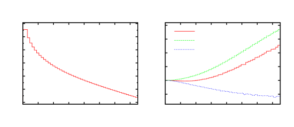
The cross section is dominated by the region close to the cut, which is reflected by the rapid decrease of the integrated cross section with increasing values for the cut on M12subscript𝑀12M_{12}. Therefore, also the corrections are dominated by the region given by the lowest accepted M12subscript𝑀12M_{12} values.

Comparing the two cross sections σ0superscript𝜎0\sigma^{0} and σQCD0subscriptsuperscript𝜎0QCD\sigma^{0}_{\mathrm{QCD}}, we find that the LO cross section with minimal cuts is predominantly given by the QCD cross section and that the electroweak effects (δEWtreesubscriptsuperscript𝛿treeEW\delta^{\text{tree}}_{\mathrm{EW}}) typically stay below the per-cent level. However, we observe a steady increase in δEWtreesubscriptsuperscript𝛿treeEW\delta^{\text{tree}}_{\mathrm{EW}} with higher M12subscript𝑀12M_{12}, which can be explained by the parton luminosities at the LHC:

1010superscript101010^{-10}108superscript10810^{-8}106superscript10610^{-6}104superscript10410^{-4}102superscript10210^{-2}100superscript10010^{0}102superscript10210^{2}104superscript10410^{4}00500500500100010001000150015001500200020002000250025002500300030003000

\makebox(0.0,0.0)[]{{}}

M12[GeV]subscript𝑀12delimited-[]GeVM_{12}\;[\mathrm{GeV}]dσ0/dM12[nb/GeV]dsuperscript𝜎0dsubscript𝑀12delimited-[]nbGeV\mathrm{d}\sigma^{0}/\mathrm{d}M_{12}\;[\mathrm{nb}/\mathrm{GeV}]ppjj+Xpp𝑗𝑗𝑋\mathrm{p}\mathrm{p}\longrightarrow jj+Xs=7TeV𝑠7TeV\sqrt{s}=7\leavevmode\nobreak\ \mathrm{TeV}0010101020202030303040404050505060606070707080808000500500500100010001000150015001500200020002000250025002500300030003000

\makebox(0.0,0.0)[]{{}}

M12[GeV]subscript𝑀12delimited-[]GeVM_{12}\;[\mathrm{GeV}]δtree[%]\delta^{\text{tree}}\;[\%]Refer to captiongg𝑔𝑔gggq𝑔𝑞gqgq¯𝑔¯𝑞g\bar{q}qq𝑞𝑞qqqq¯𝑞¯𝑞q\bar{q}q¯q¯¯𝑞¯𝑞\bar{q}\bar{q}\sum
108superscript10810^{-8}106superscript10610^{-6}104superscript10410^{-4}102superscript10210^{-2}100superscript10010^{0}102superscript10210^{2}104superscript10410^{4}00500500500100010001000150015001500200020002000250025002500300030003000

\makebox(0.0,0.0)[]{{}}

M12[GeV]subscript𝑀12delimited-[]GeVM_{12}\;[\mathrm{GeV}]dσ0/dM12[nb/GeV]dsuperscript𝜎0dsubscript𝑀12delimited-[]nbGeV\mathrm{d}\sigma^{0}/\mathrm{d}M_{12}\;[\mathrm{nb}/\mathrm{GeV}]ppjj+Xpp𝑗𝑗𝑋\mathrm{p}\mathrm{p}\longrightarrow jj+Xs=8TeV𝑠8TeV\sqrt{s}=8\leavevmode\nobreak\ \mathrm{TeV}0010101020202030303040404050505060606070707080808000500500500100010001000150015001500200020002000250025002500300030003000

\makebox(0.0,0.0)[]{{}}

M12[GeV]subscript𝑀12delimited-[]GeVM_{12}\;[\mathrm{GeV}]δtree[%]\delta^{\text{tree}}\;[\%]Refer to captiongg𝑔𝑔gggq𝑔𝑞gqgq¯𝑔¯𝑞g\bar{q}qq𝑞𝑞qqqq¯𝑞¯𝑞q\bar{q}q¯q¯¯𝑞¯𝑞\bar{q}\bar{q}\sum
1010superscript101010^{-10}108superscript10810^{-8}106superscript10610^{-6}104superscript10410^{-4}102superscript10210^{-2}100superscript10010^{0}102superscript10210^{2}104superscript10410^{4}00100010001000200020002000300030003000400040004000500050005000600060006000

\makebox(0.0,0.0)[]{{}}

M12[GeV]subscript𝑀12delimited-[]GeVM_{12}\;[\mathrm{GeV}]dσ0/dM12[nb/GeV]dsuperscript𝜎0dsubscript𝑀12delimited-[]nbGeV\mathrm{d}\sigma^{0}/\mathrm{d}M_{12}\;[\mathrm{nb}/\mathrm{GeV}]ppjj+Xpp𝑗𝑗𝑋\mathrm{p}\mathrm{p}\longrightarrow jj+Xs=14TeV𝑠14TeV\sqrt{s}=14\leavevmode\nobreak\ \mathrm{TeV}0010101020202030303040404050505060606070707080808000100010001000200020002000300030003000400040004000500050005000600060006000

\makebox(0.0,0.0)[]{{}}

M12[GeV]subscript𝑀12delimited-[]GeVM_{12}\;[\mathrm{GeV}]δtree[%]\delta^{\text{tree}}\;[\%]Refer to captiongg𝑔𝑔gggq𝑔𝑞gqgq¯𝑔¯𝑞g\bar{q}qq𝑞𝑞qqqq¯𝑞¯𝑞q\bar{q}q¯q¯¯𝑞¯𝑞\bar{q}\bar{q}\sum
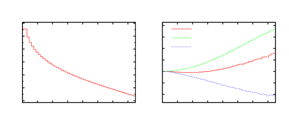
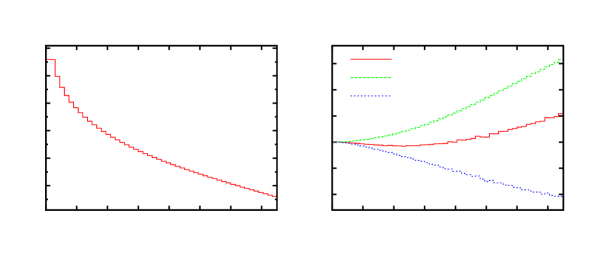
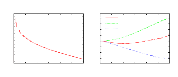
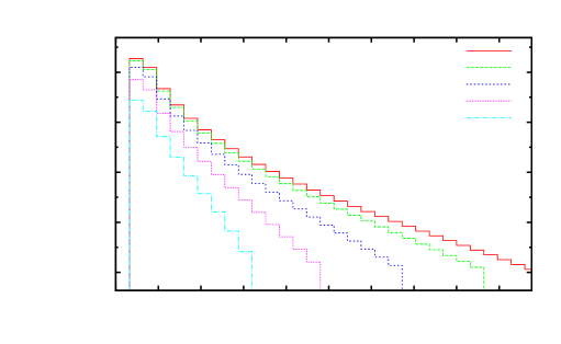
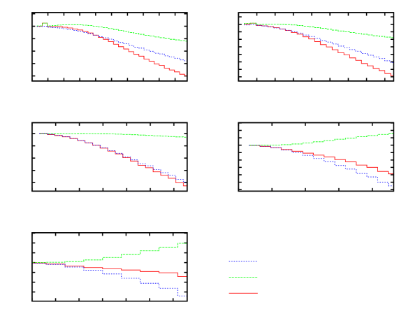
Figure 8: The LO contributions to the dijet invariant mass M12subscript𝑀12M_{12} distribution from the different initial-state parton combinations at the LHC with CM energies 7 TeVTeV\mathrm{TeV}, 8 TeVTeV\mathrm{TeV}, and 14 TeVTeV\mathrm{TeV}. Left: absolute predictions; right: relative contributions δtreesuperscript𝛿tree\delta^{\text{tree}}.

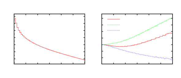
As can be seen from Fig. 8, the LO cross section is dominated at lower M12subscript𝑀12M_{12} by the gg𝑔𝑔gg- and gq𝑔𝑞gq-initiated processes, for which δEWtreesubscriptsuperscript𝛿treeEW\delta^{\text{tree}}_{\mathrm{EW}} vanishes. At higher M12subscript𝑀12M_{12}, the qq𝑞𝑞qq-initiated processes with δEWtree0subscriptsuperscript𝛿treeEW0\delta^{\text{tree}}_{\mathrm{EW}}\neq 0 become dominant, leading to the behaviour described above. The running of the strong coupling also acts in favour of increasing δEWtreesubscriptsuperscript𝛿treeEW\delta^{\text{tree}}_{\mathrm{EW}} with higher cuts on M12subscript𝑀12M_{12}. Comparing the distributions in Fig. 8 for s=7TeV𝑠7TeV\sqrt{s}=7\leavevmode\nobreak\ \mathrm{TeV} and 14TeV14TeV14\leavevmode\nobreak\ \mathrm{TeV} we observe a shift of the transition region from gg𝑔𝑔gg- to qq𝑞𝑞qq-domination from 1.5TeVsimilar-toabsent1.5TeV\sim 1.5\leavevmode\nobreak\ \mathrm{TeV} to 3TeVsimilar-toabsent3TeV\sim 3\leavevmode\nobreak\ \mathrm{TeV}, respectively. This trend is due to the fact that lower values of s𝑠\sqrt{s} require larger partonic momentum fractions x𝑥x for a fixed value of M12subscript𝑀12M_{12}, and the (valence) quark PDFs are enhanced over the gluon PDF for larger x𝑥x. This also explains the s𝑠\sqrt{s} dependence of the EW contribution δEWtreesubscriptsuperscript𝛿treeEW\delta^{\text{tree}}_{\mathrm{EW}}, which decreases with higher CM energies for the same cut on M12subscript𝑀12M_{12}.

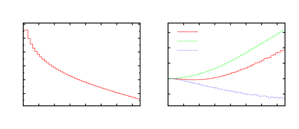
The purely weak corrections are negative throughout and increase in magnitude from 0.02%percent0.02-0.02\% to 3.6%percent3.6-3.6\% in case of the s=7TeV𝑠7TeV\sqrt{s}=7\leavevmode\nobreak\ \mathrm{TeV} setup for a M12subscript𝑀12M_{12} cut of 50GeV50GeV50\leavevmode\nobreak\ \mathrm{GeV} and 3TeV3TeV3\leavevmode\nobreak\ \mathrm{TeV}, respectively. This behaviour partly originates from the corrections containing weak logarithms ln(MW2Q2)superscriptsubscript𝑀W2superscript𝑄2\ln\left(\frac{M_{\mathrm{W}}^{2}}{Q^{2}}\right), which become larger by effectively restricting the cross section to higher energy scales Q𝑄Q via increasing cuts on the invariant mass.

Compared to δEWtreesubscriptsuperscript𝛿treeEW\delta^{\text{tree}}_{\mathrm{EW}}, the relative weak corrections δweak1-loopsubscriptsuperscript𝛿1-loopweak\delta^{\text{1-loop}}_{\mathrm{weak}} show a far weaker dependence on the CM energy. The corrections δEWtreesubscriptsuperscript𝛿treeEW\delta^{\text{tree}}_{\mathrm{EW}} and δweak1-loopsubscriptsuperscript𝛿1-loopweak\delta^{\text{1-loop}}_{\mathrm{weak}} are similar in magnitude, but of opposite sign, leading to large cancellations in the sum.

Note that the weak loop corrections δweak1-loopsubscriptsuperscript𝛿1-loopweak\delta^{\text{1-loop}}_{\mathrm{weak}} in the TeVTeV\mathrm{TeV} range are small in comparison to the typical size of the EW Sudakov factor αwπln2(MW2Q2)subscript𝛼w𝜋superscript2superscriptsubscript𝑀W2superscript𝑄2\frac{\alpha_{\mathrm{w}}}{\pi}\ln^{2}\left(\frac{M_{\mathrm{W}}^{2}}{Q^{2}}\right), which amounts to tens of per cent. This is due to the fact that also for large invariant mass M12subscript𝑀12M_{12} the cross section is not dominated by the Sudakov regime which requires that the absolute values of both partonic Mandelstam variables s^=(pa+pb)2^𝑠superscriptsubscript𝑝𝑎subscript𝑝𝑏2\hat{s}=(p_{a}+p_{b})^{2} and t^=(pakc)2^𝑡superscriptsubscript𝑝𝑎subscript𝑘𝑐2\hat{t}=(p_{a}-k_{c})^{2} are much larger than MW2superscriptsubscript𝑀W2M_{\mathrm{W}}^{2}. Instead, the cross section here is dominated by the Regge (forward) region where s^^𝑠\hat{s} is large, but |t^|^𝑡|\hat{t}| remains small.

106superscript10610^{-6}104superscript10410^{-4}102superscript10210^{-2}100superscript10010^{0}102superscript10210^{2}00500500500100010001000150015001500200020002000250025002500300030003000

\makebox(0.0,0.0)[]{{}}

M12[GeV]subscript𝑀12delimited-[]GeVM_{12}\;[\mathrm{GeV}]dσ0/dM12[nb/GeV]dsuperscript𝜎0dsubscript𝑀12delimited-[]nbGeV\mathrm{d}\sigma^{0}/\mathrm{d}M_{12}\;[\mathrm{nb}/\mathrm{GeV}]ppjj+Xpp𝑗𝑗𝑋\mathrm{p}\mathrm{p}\longrightarrow jj+Xs=7TeV𝑠7TeV\sqrt{s}=7\leavevmode\nobreak\ \mathrm{TeV}33-322-211-10011122200500500500100010001000150015001500200020002000250025002500300030003000

\makebox(0.0,0.0)[]{{}}

M12[GeV]subscript𝑀12delimited-[]GeVM_{12}\;[\mathrm{GeV}]δ[%]\delta\;[\%]Refer to captionδEWtree+δweak1-loopsubscriptsuperscript𝛿treeEWsubscriptsuperscript𝛿1-loopweak\delta^{\text{tree}}_{\mathrm{EW}}{+}\delta^{\text{1-loop}}_{\mathrm{weak}}δEWtreesubscriptsuperscript𝛿treeEW\delta^{\text{tree}}_{\mathrm{EW}}δweak1-loopsubscriptsuperscript𝛿1-loopweak\delta^{\text{1-loop}}_{\mathrm{weak}}
105superscript10510^{-5}104superscript10410^{-4}103superscript10310^{-3}102superscript10210^{-2}101superscript10110^{-1}100superscript10010^{0}101superscript10110^{1}102superscript10210^{2}103superscript10310^{3}00500500500100010001000150015001500200020002000250025002500300030003000

\makebox(0.0,0.0)[]{{}}

M12[GeV]subscript𝑀12delimited-[]GeVM_{12}\;[\mathrm{GeV}]dσ0/dM12[nb/GeV]dsuperscript𝜎0dsubscript𝑀12delimited-[]nbGeV\mathrm{d}\sigma^{0}/\mathrm{d}M_{12}\;[\mathrm{nb}/\mathrm{GeV}]ppjj+Xpp𝑗𝑗𝑋\mathrm{p}\mathrm{p}\longrightarrow jj+Xs=8TeV𝑠8TeV\sqrt{s}=8\leavevmode\nobreak\ \mathrm{TeV}33-322-211-10011122200500500500100010001000150015001500200020002000250025002500300030003000

\makebox(0.0,0.0)[]{{}}

M12[GeV]subscript𝑀12delimited-[]GeVM_{12}\;[\mathrm{GeV}]δ[%]\delta\;[\%]Refer to captionδEWtree+δweak1-loopsubscriptsuperscript𝛿treeEWsubscriptsuperscript𝛿1-loopweak\delta^{\text{tree}}_{\mathrm{EW}}{+}\delta^{\text{1-loop}}_{\mathrm{weak}}δEWtreesubscriptsuperscript𝛿treeEW\delta^{\text{tree}}_{\mathrm{EW}}δweak1-loopsubscriptsuperscript𝛿1-loopweak\delta^{\text{1-loop}}_{\mathrm{weak}}
106superscript10610^{-6}104superscript10410^{-4}102superscript10210^{-2}100superscript10010^{0}102superscript10210^{2}104superscript10410^{4}00100010001000200020002000300030003000400040004000500050005000600060006000

\makebox(0.0,0.0)[]{{}}

M12[GeV]subscript𝑀12delimited-[]GeVM_{12}\;[\mathrm{GeV}]dσ0/dM12[nb/GeV]dsuperscript𝜎0dsubscript𝑀12delimited-[]nbGeV\mathrm{d}\sigma^{0}/\mathrm{d}M_{12}\;[\mathrm{nb}/\mathrm{GeV}]ppjj+Xpp𝑗𝑗𝑋\mathrm{p}\mathrm{p}\longrightarrow jj+Xs=14TeV𝑠14TeV\sqrt{s}=14\leavevmode\nobreak\ \mathrm{TeV}66-644-422-20022200100010001000200020002000300030003000400040004000500050005000600060006000

\makebox(0.0,0.0)[]{{}}

M12[GeV]subscript𝑀12delimited-[]GeVM_{12}\;[\mathrm{GeV}]δ[%]\delta\;[\%]Refer to captionδEWtree+δweak1-loopsubscriptsuperscript𝛿treeEWsubscriptsuperscript𝛿1-loopweak\delta^{\text{tree}}_{\mathrm{EW}}{+}\delta^{\text{1-loop}}_{\mathrm{weak}}δEWtreesubscriptsuperscript𝛿treeEW\delta^{\text{tree}}_{\mathrm{EW}}δweak1-loopsubscriptsuperscript𝛿1-loopweak\delta^{\text{1-loop}}_{\mathrm{weak}}
Figure 9: Differential distributions with respect to the dijet invariant mass M12subscript𝑀12M_{12} at the LHC with CM energies 7 TeVTeV\mathrm{TeV}, 8 TeVTeV\mathrm{TeV}, and 14 TeVTeV\mathrm{TeV}. Left: absolute predictions; right: relative contributions δ𝛿\delta.

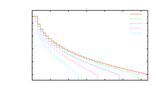
This feature is also evident in the dijet invariant-mass distributions shown in Fig. 9. The relative corrections given in Table 1 are almost identical to the corrections in Fig. 9 at the respective cut value of M12subscript𝑀12M_{12}, since the corrections are dominated by the region close to the cut.

106superscript10610^{-6}104superscript10410^{-4}102superscript10210^{-2}100superscript10010^{0}102superscript10210^{2}00500500500100010001000150015001500200020002000250025002500

\makebox(0.0,0.0)[]{{}}

M12[GeV]subscript𝑀12delimited-[]GeVM_{12}\;[\mathrm{GeV}]d2σ0/(dM12dy)[nb/GeV]superscriptd2superscript𝜎0dsubscript𝑀12dsuperscript𝑦delimited-[]nbGeV\mathrm{d}^{2}\sigma^{0}/(\mathrm{d}M_{12}\,\mathrm{d}y^{*})\;[\mathrm{nb}/\mathrm{GeV}]ppjj+Xpp𝑗𝑗𝑋\mathrm{p}\mathrm{p}\longrightarrow jj+Xs=8TeV𝑠8TeV\sqrt{s}=8\leavevmode\nobreak\ \mathrm{TeV}Refer to captiony<0.5superscript𝑦0.5y^{*}<0.50.5<y<1.00.5superscript𝑦1.00.5<y^{*}<1.01.0<y<1.51.0superscript𝑦1.51.0<y^{*}<1.51.5<y<2.01.5superscript𝑦2.01.5<y^{*}<2.02.0<y<2.52.0superscript𝑦2.52.0<y^{*}<2.5
1010-1055-50055510101015151520202000500500500100010001000150015001500200020002000250025002500

\makebox(0.0,0.0)[]{{}}

M12[GeV]subscript𝑀12delimited-[]GeVM_{12}\;[\mathrm{GeV}]

δ[%]\delta\;[\%]

y<0.5superscript𝑦0.5y^{*}<0.588-866-644-422-20022244466688800500500500100010001000150015001500200020002000250025002500

\makebox(0.0,0.0)[]{{}}

M12[GeV]subscript𝑀12delimited-[]GeVM_{12}\;[\mathrm{GeV}]

δ[%]\delta\;[\%]

0.5<y<1.00.5superscript𝑦1.00.5<y^{*}<1.066-644-422-20022244400500500500100010001000150015001500200020002000250025002500

\makebox(0.0,0.0)[]{{}}

M12[GeV]subscript𝑀12delimited-[]GeVM_{12}\;[\mathrm{GeV}]

δ[%]\delta\;[\%]

1.0<y<1.51.0superscript𝑦1.51.0<y^{*}<1.544-433-322-211-10011122233300500500500100010001000150015001500200020002000250025002500

\makebox(0.0,0.0)[]{{}}

M12[GeV]subscript𝑀12delimited-[]GeVM_{12}\;[\mathrm{GeV}]

δ[%]\delta\;[\%]

1.5<y<2.01.5superscript𝑦2.01.5<y^{*}<2.022-211-10011122200500500500100010001000150015001500200020002000250025002500

\makebox(0.0,0.0)[]{{}}

M12[GeV]subscript𝑀12delimited-[]GeVM_{12}\;[\mathrm{GeV}]

δ[%]\delta\;[\%]

ppjj+Xats=8TeVpp𝑗𝑗𝑋at𝑠8TeV\mathrm{p}\mathrm{p}\longrightarrow jj+X\;\mbox{at}\;\sqrt{s}=8\leavevmode\nobreak\ \mathrm{TeV}2.0<y<2.52.0superscript𝑦2.52.0<y^{*}<2.5Refer to captionδEWtree+δweak1-loopsubscriptsuperscript𝛿treeEWsubscriptsuperscript𝛿1-loopweak\delta^{\text{tree}}_{\mathrm{EW}}{+}\delta^{\text{1-loop}}_{\mathrm{weak}}δEWtreesubscriptsuperscript𝛿treeEW\delta^{\text{tree}}_{\mathrm{EW}}δweak1-loopsubscriptsuperscript𝛿1-loopweak\delta^{\text{1-loop}}_{\mathrm{weak}}
Figure 10: Double-differential distribution with respect to the dijet invariant mass M12subscript𝑀12M_{12} and ysuperscript𝑦y^{*} at the LHC with a CM energy of 8 TeVTeV\mathrm{TeV}. In the absolute prediction (uppermost plot) the cross section is divided by the bin width in ysuperscript𝑦y^{*}.
108superscript10810^{-8}106superscript10610^{-6}104superscript10410^{-4}102superscript10210^{-2}100superscript10010^{0}102superscript10210^{2}104superscript10410^{4}00100010001000200020002000300030003000400040004000500050005000

\makebox(0.0,0.0)[]{{}}

M12[GeV]subscript𝑀12delimited-[]GeVM_{12}\;[\mathrm{GeV}]d2σ0/(dM12dy)[nb/GeV]superscriptd2superscript𝜎0dsubscript𝑀12dsuperscript𝑦delimited-[]nbGeV\mathrm{d}^{2}\sigma^{0}/(\mathrm{d}M_{12}\,\mathrm{d}y^{*})\;[\mathrm{nb}/\mathrm{GeV}]ppjj+Xpp𝑗𝑗𝑋\mathrm{p}\mathrm{p}\longrightarrow jj+Xs=14TeV𝑠14TeV\sqrt{s}=14\leavevmode\nobreak\ \mathrm{TeV}Refer to captiony<0.5superscript𝑦0.5y^{*}<0.50.5<y<1.00.5superscript𝑦1.00.5<y^{*}<1.01.0<y<1.51.0superscript𝑦1.51.0<y^{*}<1.51.5<y<2.01.5superscript𝑦2.01.5<y^{*}<2.02.0<y<2.52.0superscript𝑦2.52.0<y^{*}<2.5
1515-151010-1055-50055510101015151520202025252500100010001000200020002000300030003000400040004000500050005000

\makebox(0.0,0.0)[]{{}}

M12[GeV]subscript𝑀12delimited-[]GeVM_{12}\;[\mathrm{GeV}]

δ[%]\delta\;[\%]

y<0.5superscript𝑦0.5y^{*}<0.51010-1055-50055510101000100010001000200020002000300030003000400040004000500050005000

\makebox(0.0,0.0)[]{{}}

M12[GeV]subscript𝑀12delimited-[]GeVM_{12}\;[\mathrm{GeV}]

δ[%]\delta\;[\%]

0.5<y<1.00.5superscript𝑦1.00.5<y^{*}<1.01010-1088-866-644-422-20022244466600100010001000200020002000300030003000400040004000500050005000

\makebox(0.0,0.0)[]{{}}

M12[GeV]subscript𝑀12delimited-[]GeVM_{12}\;[\mathrm{GeV}]

δ[%]\delta\;[\%]

1.0<y<1.51.0superscript𝑦1.51.0<y^{*}<1.566-644-422-20022244400100010001000200020002000300030003000400040004000500050005000

\makebox(0.0,0.0)[]{{}}

M12[GeV]subscript𝑀12delimited-[]GeVM_{12}\;[\mathrm{GeV}]

δ[%]\delta\;[\%]

1.5<y<2.01.5superscript𝑦2.01.5<y^{*}<2.055-544-433-322-211-10011122233300100010001000200020002000300030003000400040004000500050005000

\makebox(0.0,0.0)[]{{}}

M12[GeV]subscript𝑀12delimited-[]GeVM_{12}\;[\mathrm{GeV}]

δ[%]\delta\;[\%]

ppjj+Xats=14TeVpp𝑗𝑗𝑋at𝑠14TeV\mathrm{p}\mathrm{p}\longrightarrow jj+X\;\mbox{at}\;\sqrt{s}=14\leavevmode\nobreak\ \mathrm{TeV}2.0<y<2.52.0superscript𝑦2.52.0<y^{*}<2.5Refer to captionδEWtree+δweak1-loopsubscriptsuperscript𝛿treeEWsubscriptsuperscript𝛿1-loopweak\delta^{\text{tree}}_{\mathrm{EW}}{+}\delta^{\text{1-loop}}_{\mathrm{weak}}δEWtreesubscriptsuperscript𝛿treeEW\delta^{\text{tree}}_{\mathrm{EW}}δweak1-loopsubscriptsuperscript𝛿1-loopweak\delta^{\text{1-loop}}_{\mathrm{weak}}
Figure 11: Same as in Fig. 10, but for a CM energy of 14 TeVTeV\mathrm{TeV}.

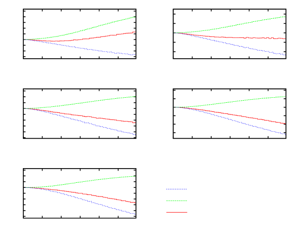
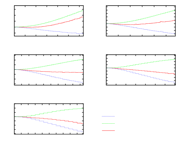
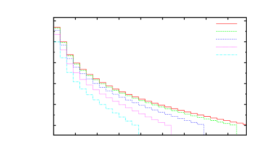
Figures 10 and 11 show the results for the M12subscript𝑀12M_{12} distributions corresponding to different rapidity ranges. Specifically, the phase space is divided into different regions of ysuperscript𝑦y^{*}, which is defined as half the rapidity difference of the two leading jets,

y=|y1y2|2.superscript𝑦subscript𝑦1subscript𝑦22y^{*}=\frac{\lvert y_{1}-y_{2}\rvert}{2}. (3.9)

For the binning in ysuperscript𝑦y^{*} we have chosen five bins of equal width covering the range 0<y<2.50superscript𝑦2.50<y^{*}<2.5. In all ysuperscript𝑦y^{*} bins we observe the above described behaviour of the relative corrections that increase in magnitude with higher invariant mass, where the tree-level EW contributions and the radiative weak corrections give positive and negative contributions, respectively. Furthermore, a strong dependence on ysuperscript𝑦y^{*} is observed, such that both, δEWtreesubscriptsuperscript𝛿treeEW\delta^{\text{tree}}_{\mathrm{EW}} and δweak1-loopsubscriptsuperscript𝛿1-loopweak\delta^{\text{1-loop}}_{\mathrm{weak}}, are larger for smaller values of ysuperscript𝑦y^{*}. For s=8TeV𝑠8TeV\sqrt{s}=8\leavevmode\nobreak\ \mathrm{TeV} and the invariant mass of 3TeV3TeV3\leavevmode\nobreak\ \mathrm{TeV} the corrections δEWtreesubscriptsuperscript𝛿treeEW\delta^{\text{tree}}_{\mathrm{EW}} and δweak1-loopsubscriptsuperscript𝛿1-loopweak\delta^{\text{1-loop}}_{\mathrm{weak}} in the first bin (y<0.5superscript𝑦0.5y^{*}<0.5) amount to approximately 15%percent1515\% and 10%percent10-10\%, respectively, whereas in the highest ysuperscript𝑦y^{*}-bin (2<y<2.52superscript𝑦2.52<y^{*}<2.5) we observe about 1.5%percent1.51.5\% and 2.5%percent2.5-2.5\% for the respective corrections. As it is evident from the numbers quoted above, δEWtreesubscriptsuperscript𝛿treeEW\delta^{\text{tree}}_{\mathrm{EW}} decreases more rapidly than δweak1-loopsubscriptsuperscript𝛿1-loopweak\delta^{\text{1-loop}}_{\mathrm{weak}} for higher ysuperscript𝑦y^{*}. The sum of both contributions, thus, has a positive net-contribution for y<0.5superscript𝑦0.5y^{*}<0.5, gradually decreasing with higher ysuperscript𝑦y^{*} values. In the range of highest ysuperscript𝑦y^{*} (2<y<2.52superscript𝑦2.52<y^{*}<2.5), even a negative net-contribution results. Qualitatively we observe the same behaviour also at the CM energy of s=14TeV𝑠14TeV\sqrt{s}=14\leavevmode\nobreak\ \mathrm{TeV}. Here we examine dijet invariant masses up to 6TeV6TeV6\leavevmode\nobreak\ \mathrm{TeV}, where we observe approximately 20%percent2020\% and 15%percent15-15\% in the first bin (y<0.5superscript𝑦0.5y^{*}<0.5), and 2%percent22\% and 5%percent5-5\% in the highest ysuperscript𝑦y^{*}-bin (2<y<2.52superscript𝑦2.52<y^{*}<2.5) for δEWtreesubscriptsuperscript𝛿treeEW\delta^{\text{tree}}_{\mathrm{EW}} and δweak1-loopsubscriptsuperscript𝛿1-loopweak\delta^{\text{1-loop}}_{\mathrm{weak}}, respectively.

As already indicated in the discussion of integrated cross sections above, the behaviour of the corrections can be better understood by identifying the Sudakov regime in phase space. For the contributions with 22222\rightarrow 2 kinematics, i.e. the LO cross sections and the virtual corrections, the following relations hold:

|y^1|=|y^2|=y,s^=M122,t^=M1221+e±2y,u^=M1221+e2y,formulae-sequencesubscript^𝑦1subscript^𝑦2superscript𝑦formulae-sequence^𝑠superscriptsubscript𝑀122formulae-sequence^𝑡superscriptsubscript𝑀1221superscripteplus-or-minus2superscript𝑦^𝑢superscriptsubscript𝑀1221superscripteminus-or-plus2superscript𝑦\lvert\hat{y}_{1}\rvert=\lvert-\hat{y}_{2}\rvert=y^{*},\quad\hat{s}=M_{12}^{2},\quad\hat{t}=-\frac{M_{12}^{2}}{1+\mathrm{e}^{\pm 2y^{*}}},\quad\hat{u}=-\frac{M_{12}^{2}}{1+\mathrm{e}^{\mp 2y^{*}}}, (3.10)

where y^isubscript^𝑦𝑖\hat{y}_{i} and s^^𝑠\hat{s}, t^^𝑡\hat{t}, u^^𝑢\hat{u} denote the rapidity and the partonic Mandelstam variables. The two different signs refer to y^10greater-than-or-less-thansubscript^𝑦10\hat{y}_{1}\gtrless 0. For large M12MWmuch-greater-thansubscript𝑀12subscript𝑀WM_{12}\gg M_{\mathrm{W}} and small ysuperscript𝑦y^{*} we reside in the Sudakov regime, where all scales are simultaneously large compared to the vector-boson masses. Here, all logarithms of the form αwln2(Q2/MV2)subscript𝛼wsuperscript2superscript𝑄2superscriptsubscript𝑀𝑉2\alpha_{\mathrm{w}}\ln^{2}\left(Q^{2}/M_{V}^{2}\right), with Q2=s^,t^,u^superscript𝑄2^𝑠^𝑡^𝑢Q^{2}=\hat{s},-\hat{t},-\hat{u} become large, leading to the observed enhancements of the weak radiative corrections. As can be seen in the absolute distributions in Figs. 10 and 11, however, this regime delivers only a small fraction to the cross section if the high-energy region is defined via cuts on the invariant mass M12subscript𝑀12M_{12}.

Although the corrections δEWtreesubscriptsuperscript𝛿treeEW\delta^{\text{tree}}_{\mathrm{EW}} show a similar behaviour, their origin is of a completely different nature: As discussed above, the bulk of the contributions to δEWtreesubscriptsuperscript𝛿treeEW\delta^{\text{tree}}_{\mathrm{EW}} originate from the qq𝑞𝑞qq-initiated processes, in particular from the partonic subprocesses uuuuuuuu\mathrm{u}\mathrm{u}\rightarrow\mathrm{u}\mathrm{u} and udududud\mathrm{u}\mathrm{d}\rightarrow\mathrm{u}\mathrm{d}. Owing to their colour structure, the interference terms of 𝒪(αsα)𝒪subscript𝛼s𝛼{\mathcal{O}\left(\alpha_{\mathrm{s}}\alpha\right)} considered here receive contributions from products of t𝑡t-, u𝑢u-, and s𝑠s-channel diagrams only, but not from squares of those topologies. Therefore, these interferences appear to be more central than the larger LO QCD contributions which are dominated by squared topologies.

In summary, for high M12subscript𝑀12M_{12}, where the corrections are largest, the cross section is dominated by the contribution coming from the highest possible ysuperscript𝑦y^{*} values. However, this region receives the smallest corrections, leading to the small corrections that we observe in Table 1 even for very high M12subscript𝑀12M_{12} cuts. As we will see in the next section, this behaviour is reversed in case of the transverse-momentum distributions. Despite the different origin of the relative corrections δweak1-loopsubscriptsuperscript𝛿1-loopweak\delta^{\text{1-loop}}_{\mathrm{weak}} and δEWtreesubscriptsuperscript𝛿treeEW\delta^{\text{tree}}_{\mathrm{EW}}, they conspire together to large cancellations in the sum δEWtree+δweak1-loopsubscriptsuperscript𝛿treeEWsubscriptsuperscript𝛿1-loopweak\delta^{\text{tree}}_{\mathrm{EW}}{+}\delta^{\text{1-loop}}_{\mathrm{weak}}. The degree of this compensation, however, depends on the chosen cuts defining the observable.

3.3.2 The transverse momenta of the leading and subleading jet at the LHC

ppjj+Xats=7TeVkT,1/GeV255010020050010001500σ0/nb78600(2)5417.1(1)291.205(9)11.1765(2)63.697(2)103396.843(8)1065.9746(10)106σQCD0/nb78561(2)5413.8(2)290.517(9)11.0873(3)61.251(2)103353.47(1)1064.9611(9)106δweak1-loop/%0.020.100.340.992.965.126.13δEWtree/%0.050.060.240.803.9912.2820.44δ/%0.020.040.100.191.047.1614.31σNLO/nb78581(2)5411.9(1)290.216(9)11.0664(3)61.887(4)103378.76(4)1065.6705(8)106\begin{array}[]{c|c c c c c c c }\lx@intercol\hfil\mathrm{p}\mathrm{p}\longrightarrow jj+X\;\mbox{at}\;\sqrt{s}=7\leavevmode\nobreak\ \mathrm{TeV}\hfil\lx@intercol\\ \hline\cr k_{\mathrm{T},1}/\mathrm{GeV}&25-\infty&50-\infty&100-\infty&200-\infty&500-\infty&1000-\infty&1500-\infty\\ \hline\cr\sigma^{0}/\mathrm{nb}&78600(2)&5417.1(1)&291.205(9)&11.1765(2)&63.697(2)\cdot 10^{-3}&396.843(8)\cdot 10^{-6}&5.9746(10)\cdot 10^{-6}\\ \sigma^{0}_{\mathrm{QCD}}/\mathrm{nb}&78561(2)&5413.8(2)&290.517(9)&11.0873(3)&61.251(2)\cdot 10^{-3}&353.47(1)\cdot 10^{-6}&4.9611(9)\cdot 10^{-6}\\ \hline\cr\delta^{\text{1-loop}}_{\mathrm{weak}}/\%&-0.02&-0.10&-0.34&-0.99&-2.96&-5.12&-6.13\\ \delta^{\text{tree}}_{\mathrm{EW}}/\%&0.05&0.06&0.24&0.80&3.99&12.28&20.44\\ \sum\delta/\%&0.02&-0.04&-0.10&-0.19&1.04&7.16&14.31\\ \hline\cr\sigma^{\mathrm{NLO}}/\mathrm{nb}&78581(2)&5411.9(1)&290.216(9)&11.0664(3)&61.887(4)\cdot 10^{-3}&378.76(4)\cdot 10^{-6}&5.6705(8)\cdot 10^{-6}\end{array}
ppjj+Xats=8TeVkT,1/GeV255010020050010001500σ0/nb94683(2)6762.3(2)380.68(1)15.7387(5)105.965(3)103877.88(2)10620.4538(3)106σQCD0/nb94638(2)6759.0(3)379.90(1)15.6330(6)102.626(2)103795.70(3)10617.3482(2)106δweak1-loop/%0.020.090.330.972.965.356.70δEWtree/%0.040.050.210.683.2610.3317.90δ/%0.020.040.120.290.304.9811.20σNLO/nb94661(2)6756.1(2)379.44(1)15.5871(6)102.932(5)103835.29(9)10619.292(3)106\begin{array}[]{c|c c c c c c c }\lx@intercol\hfil\mathrm{p}\mathrm{p}\longrightarrow jj+X\;\mbox{at}\;\sqrt{s}=8\leavevmode\nobreak\ \mathrm{TeV}\hfil\lx@intercol\\ \hline\cr k_{\mathrm{T},1}/\mathrm{GeV}&25-\infty&50-\infty&100-\infty&200-\infty&500-\infty&1000-\infty&1500-\infty\\ \hline\cr\sigma^{0}/\mathrm{nb}&94683(2)&6762.3(2)&380.68(1)&15.7387(5)&105.965(3)\cdot 10^{-3}&877.88(2)\cdot 10^{-6}&20.4538(3)\cdot 10^{-6}\\ \sigma^{0}_{\mathrm{QCD}}/\mathrm{nb}&94638(2)&6759.0(3)&379.90(1)&15.6330(6)&102.626(2)\cdot 10^{-3}&795.70(3)\cdot 10^{-6}&17.3482(2)\cdot 10^{-6}\\ \hline\cr\delta^{\text{1-loop}}_{\mathrm{weak}}/\%&-0.02&-0.09&-0.33&-0.97&-2.96&-5.35&-6.70\\ \delta^{\text{tree}}_{\mathrm{EW}}/\%&0.04&0.05&0.21&0.68&3.26&10.33&17.90\\ \sum\delta/\%&0.02&-0.04&-0.12&-0.29&0.30&4.98&11.20\\ \hline\cr\sigma^{\mathrm{NLO}}/\mathrm{nb}&94661(2)&6756.1(2)&379.44(1)&15.5871(6)&102.932(5)\cdot 10^{-3}&835.29(9)\cdot 10^{-6}&19.292(3)\cdot 10^{-6}\end{array}
ppjj+Xats=14TeVkT,1/GeV255010020050010002500σ0/nb198483(4)16194.3(5)1074.11(3)56.405(2)671.10(2)10312.0383(4)1038.8504(2)106σQCD0/nb198410(5)16189.7(5)1072.85(4)56.204(1)661.52(2)10311.5060(2)1037.4826(2)106δweak1-loop/%0.020.080.280.842.725.4810.49δEWtree/%0.030.030.120.361.444.6218.28δ/%0.010.050.150.481.280.867.79σNLO/nb198443(4)16181.6(5)1071.15(3)55.935(2)653.10(3)10311.4076(10)1038.066(1)106\begin{array}[]{c|c c c c c c c }\lx@intercol\hfil\mathrm{p}\mathrm{p}\longrightarrow jj+X\;\mbox{at}\;\sqrt{s}=14\leavevmode\nobreak\ \mathrm{TeV}\hfil\lx@intercol\\ \hline\cr k_{\mathrm{T},1}/\mathrm{GeV}&25-\infty&50-\infty&100-\infty&200-\infty&500-\infty&1000-\infty&2500-\infty\\ \hline\cr\sigma^{0}/\mathrm{nb}&198483(4)&16194.3(5)&1074.11(3)&56.405(2)&671.10(2)\cdot 10^{-3}&12.0383(4)\cdot 10^{-3}&8.8504(2)\cdot 10^{-6}\\ \sigma^{0}_{\mathrm{QCD}}/\mathrm{nb}&198410(5)&16189.7(5)&1072.85(4)&56.204(1)&661.52(2)\cdot 10^{-3}&11.5060(2)\cdot 10^{-3}&7.4826(2)\cdot 10^{-6}\\ \hline\cr\delta^{\text{1-loop}}_{\mathrm{weak}}/\%&-0.02&-0.08&-0.28&-0.84&-2.72&-5.48&-10.49\\ \delta^{\text{tree}}_{\mathrm{EW}}/\%&0.03&0.03&0.12&0.36&1.44&4.62&18.28\\ \sum\delta/\%&0.01&-0.05&-0.15&-0.48&-1.28&-0.86&7.79\\ \hline\cr\sigma^{\mathrm{NLO}}/\mathrm{nb}&198443(4)&16181.6(5)&1071.15(3)&55.935(2)&653.10(3)\cdot 10^{-3}&11.4076(10)\cdot 10^{-3}&8.066(1)\cdot 10^{-6}\end{array}
Table 2: Integrated dijet cross sections and respective corrections for various ranges of the transverse momentum of the leading jet kT,1subscript𝑘T1k_{\mathrm{T},1} at the LHC with CM energies 7 TeVTeV\mathrm{TeV}, 8 TeVTeV\mathrm{TeV}, and 14 TeVTeV\mathrm{TeV}.

In Table 2 we list the various integrated cross sections at LO, the NLO cross section, and the correction factors defined above for different cuts on the transverse momentum of the leading jet, kT,1subscript𝑘T1k_{\mathrm{T},1}. The cut kT,1>25GeVsubscript𝑘T125GeVk_{\mathrm{T},1}>25\leavevmode\nobreak\ \mathrm{GeV} in the first column is already imposed by the default set of cuts and does not represent a further restriction to the cross section. Again, the integrated cross section decreases rapidly with more restrictive cuts on the transverse momentum, indicating that the cross section, and with it the corrections, are dominated by the region with the lowest accepted kT,1subscript𝑘T1k_{\mathrm{T},1}.

The weak radiative corrections display the expected Sudakov-type behaviour with increasing negative corrections for higher kT,1subscript𝑘T1k_{\mathrm{T},1}-cuts and only a modest dependence on the CM energy of the collider. For cut values of 25GeV25GeV25\leavevmode\nobreak\ \mathrm{GeV} up to 1.5TeV1.5TeV1.5\leavevmode\nobreak\ \mathrm{TeV} they increase from 0.02%percent0.02-0.02\% to 6%percent6-6\% for s=7TeV𝑠7TeV\sqrt{s}=7\leavevmode\nobreak\ \mathrm{TeV}. For s=14TeV𝑠14TeV\sqrt{s}=14\leavevmode\nobreak\ \mathrm{TeV} and a cut of kT,1>2.5TeVsubscript𝑘T12.5TeVk_{\mathrm{T},1}>2.5\leavevmode\nobreak\ \mathrm{TeV} the radiative corrections even amount to 11%percent11-11\%. The LO EW contributions show a much stronger dependence on the collider energy than the loop corrections, in particular for more restrictive cuts. This s𝑠\sqrt{s} dependence is also stronger than the one observed for the dijet invariant-mass spectra discussed in the previous section.

Considering that kT,1M12/2subscript𝑘T1subscript𝑀122k_{\mathrm{T},1}\leq M_{12}/2 at LO and that the cross section as well as the corrections are dominated by the region of lowest accepted M12subscript𝑀12M_{12}, one might naively expect that the results for a fixed cut on kT,1subscript𝑘T1k_{\mathrm{T},1} should be comparable to the respective corrections for a M12subscript𝑀12M_{12} cut of twice that value. However, the region close to M122kT,1subscript𝑀122subscript𝑘T1M_{12}\approx 2k_{\mathrm{T},1} at LO requires central jet production in the partonic CM frame, i.e. y0superscript𝑦0y^{*}\approx 0, so that the cross section defined via the kT,1subscript𝑘T1k_{\mathrm{T},1} cut is dominated by the Sudakov regime. This explains the smaller cross section and the larger corrections as compared to the cross section defined via the corresponding M12subscript𝑀12M_{12} cut discussed in the previous section.

108superscript10810^{-8}106superscript10610^{-6}104superscript10410^{-4}102superscript10210^{-2}100superscript10010^{0}102superscript10210^{2}104superscript10410^{4}00200200200400400400600600600800800800100010001000120012001200140014001400

\makebox(0.0,0.0)[]{{}}

kT,1[GeV]subscript𝑘T1delimited-[]GeVk_{\mathrm{T},1}\;[\mathrm{GeV}]dσ0/dkT,1[nb/GeV]dsuperscript𝜎0dsubscript𝑘T1delimited-[]nbGeV\mathrm{d}\sigma^{0}/\mathrm{d}k_{\mathrm{T},1}\;[\mathrm{nb}/\mathrm{GeV}]ppjj+Xpp𝑗𝑗𝑋\mathrm{p}\mathrm{p}\longrightarrow jj+Xs=7TeV𝑠7TeV\sqrt{s}=7\leavevmode\nobreak\ \mathrm{TeV}55-50055510101015151520202000200200200400400400600600600800800800100010001000120012001200140014001400

\makebox(0.0,0.0)[]{{}}

kT,1[GeV]subscript𝑘T1delimited-[]GeVk_{\mathrm{T},1}\;[\mathrm{GeV}]δ[%]\delta\;[\%]Refer to captionδEWtree+δweak1-loopsubscriptsuperscript𝛿treeEWsubscriptsuperscript𝛿1-loopweak\delta^{\text{tree}}_{\mathrm{EW}}{+}\delta^{\text{1-loop}}_{\mathrm{weak}}δEWtreesubscriptsuperscript𝛿treeEW\delta^{\text{tree}}_{\mathrm{EW}}δweak1-loopsubscriptsuperscript𝛿1-loopweak\delta^{\text{1-loop}}_{\mathrm{weak}}
106superscript10610^{-6}104superscript10410^{-4}102superscript10210^{-2}100superscript10010^{0}102superscript10210^{2}104superscript10410^{4}00200200200400400400600600600800800800100010001000120012001200140014001400

\makebox(0.0,0.0)[]{{}}

kT,1[GeV]subscript𝑘T1delimited-[]GeVk_{\mathrm{T},1}\;[\mathrm{GeV}]dσ0/dkT,1[nb/GeV]dsuperscript𝜎0dsubscript𝑘T1delimited-[]nbGeV\mathrm{d}\sigma^{0}/\mathrm{d}k_{\mathrm{T},1}\;[\mathrm{nb}/\mathrm{GeV}]ppjj+Xpp𝑗𝑗𝑋\mathrm{p}\mathrm{p}\longrightarrow jj+Xs=8TeV𝑠8TeV\sqrt{s}=8\leavevmode\nobreak\ \mathrm{TeV}55-50055510101015151500200200200400400400600600600800800800100010001000120012001200140014001400

\makebox(0.0,0.0)[]{{}}

kT,1[GeV]subscript𝑘T1delimited-[]GeVk_{\mathrm{T},1}\;[\mathrm{GeV}]δ[%]\delta\;[\%]Refer to captionδEWtree+δweak1-loopsubscriptsuperscript𝛿treeEWsubscriptsuperscript𝛿1-loopweak\delta^{\text{tree}}_{\mathrm{EW}}{+}\delta^{\text{1-loop}}_{\mathrm{weak}}δEWtreesubscriptsuperscript𝛿treeEW\delta^{\text{tree}}_{\mathrm{EW}}δweak1-loopsubscriptsuperscript𝛿1-loopweak\delta^{\text{1-loop}}_{\mathrm{weak}}
108superscript10810^{-8}106superscript10610^{-6}104superscript10410^{-4}102superscript10210^{-2}100superscript10010^{0}102superscript10210^{2}104superscript10410^{4}00500500500100010001000150015001500200020002000250025002500300030003000

\makebox(0.0,0.0)[]{{}}

kT,1[GeV]subscript𝑘T1delimited-[]GeVk_{\mathrm{T},1}\;[\mathrm{GeV}]dσ0/dkT,1[nb/GeV]dsuperscript𝜎0dsubscript𝑘T1delimited-[]nbGeV\mathrm{d}\sigma^{0}/\mathrm{d}k_{\mathrm{T},1}\;[\mathrm{nb}/\mathrm{GeV}]ppjj+Xpp𝑗𝑗𝑋\mathrm{p}\mathrm{p}\longrightarrow jj+Xs=14TeV𝑠14TeV\sqrt{s}=14\leavevmode\nobreak\ \mathrm{TeV}1010-1055-50055510101015151520202000500500500100010001000150015001500200020002000250025002500300030003000

\makebox(0.0,0.0)[]{{}}

kT,1[GeV]subscript𝑘T1delimited-[]GeVk_{\mathrm{T},1}\;[\mathrm{GeV}]δ[%]\delta\;[\%]Refer to captionδEWtree+δweak1-loopsubscriptsuperscript𝛿treeEWsubscriptsuperscript𝛿1-loopweak\delta^{\text{tree}}_{\mathrm{EW}}{+}\delta^{\text{1-loop}}_{\mathrm{weak}}δEWtreesubscriptsuperscript𝛿treeEW\delta^{\text{tree}}_{\mathrm{EW}}δweak1-loopsubscriptsuperscript𝛿1-loopweak\delta^{\text{1-loop}}_{\mathrm{weak}}
Figure 12: Differential distributions with respect to the transverse momentum of the leading jet kT,1subscript𝑘T1k_{\mathrm{T},1} at the LHC with CM energies 7 TeVTeV\mathrm{TeV}, 8 TeVTeV\mathrm{TeV}, and 14 TeVTeV\mathrm{TeV}. Left: absolute predictions; right: relative contributions δ𝛿\delta.

The differential distributions in kT,1subscript𝑘T1k_{\mathrm{T},1} shown in Fig. 12 cover the range up to kT,1=1.5TeVsubscript𝑘T11.5TeVk_{\mathrm{T},1}=1.5\leavevmode\nobreak\ \mathrm{TeV} for s=7TeV, 8TeV𝑠7TeV8TeV\sqrt{s}=7\leavevmode\nobreak\ \mathrm{TeV},\,8\leavevmode\nobreak\ \mathrm{TeV}, and up to kT,1=3TeVsubscript𝑘T13TeVk_{\mathrm{T},1}=3\leavevmode\nobreak\ \mathrm{TeV} for s=14TeV𝑠14TeV\sqrt{s}=14\leavevmode\nobreak\ \mathrm{TeV} and further underline the observations made above. The weak corrections display the expected behaviour from the Sudakov logarithms with corrections reaching up to 6%percent6-6\% at kT,1=1.5TeVsubscript𝑘T11.5TeVk_{\mathrm{T},1}=1.5\leavevmode\nobreak\ \mathrm{TeV} for s= 7TeV, 8TeV𝑠7TeV8TeV\sqrt{s}=\leavevmode\nobreak\ 7\leavevmode\nobreak\ \mathrm{TeV},\,8\leavevmode\nobreak\ \mathrm{TeV}, and 12%percent12-12\% at kT,1=3TeVsubscript𝑘T13TeVk_{\mathrm{T},1}=3\leavevmode\nobreak\ \mathrm{TeV} for s= 14TeV𝑠14TeV\sqrt{s}=\leavevmode\nobreak\ 14\leavevmode\nobreak\ \mathrm{TeV}. On the other hand, the tree-level corrections δEWtreesubscriptsuperscript𝛿treeEW\delta^{\text{tree}}_{\mathrm{EW}} increase with higher kT,1subscript𝑘T1k_{\mathrm{T},1} and reach approximately 16%percent1616\% at kT,1=1.5TeVsubscript𝑘T11.5TeVk_{\mathrm{T},1}=1.5\leavevmode\nobreak\ \mathrm{TeV} for s= 7TeV, 8TeV𝑠7TeV8TeV\sqrt{s}=\leavevmode\nobreak\ 7\leavevmode\nobreak\ \mathrm{TeV},\,8\leavevmode\nobreak\ \mathrm{TeV}, and 20%percent2020\% at kT,1=3TeVsubscript𝑘T13TeVk_{\mathrm{T},1}=3\leavevmode\nobreak\ \mathrm{TeV} for s= 14TeV𝑠14TeV\sqrt{s}=\leavevmode\nobreak\ 14\leavevmode\nobreak\ \mathrm{TeV}, resulting in significant cancellations in the sum δEWtree+δweak1-loopsubscriptsuperscript𝛿treeEWsubscriptsuperscript𝛿1-loopweak\delta^{\text{tree}}_{\mathrm{EW}}{+}\delta^{\text{1-loop}}_{\mathrm{weak}}.

106superscript10610^{-6}104superscript10410^{-4}102superscript10210^{-2}100superscript10010^{0}102superscript10210^{2}00200200200400400400600600600800800800100010001000120012001200

\makebox(0.0,0.0)[]{{}}

kT,1[GeV]subscript𝑘T1delimited-[]GeVk_{\mathrm{T},1}\;[\mathrm{GeV}]d2σ0/(dkT,1dy)[nb/GeV]superscriptd2superscript𝜎0dsubscript𝑘T1dsuperscript𝑦delimited-[]nbGeV\mathrm{d}^{2}\sigma^{0}/(\mathrm{d}k_{\mathrm{T},1}\,\mathrm{d}y^{*})\;[\mathrm{nb}/\mathrm{GeV}]ppjj+Xpp𝑗𝑗𝑋\mathrm{p}\mathrm{p}\longrightarrow jj+Xs=8TeV𝑠8TeV\sqrt{s}=8\leavevmode\nobreak\ \mathrm{TeV}Refer to captiony<0.5superscript𝑦0.5y^{*}<0.50.5<y<1.00.5superscript𝑦1.00.5<y^{*}<1.01.0<y<1.51.0superscript𝑦1.51.0<y^{*}<1.51.5<y<2.01.5superscript𝑦2.01.5<y^{*}<2.02.0<y<2.52.0superscript𝑦2.52.0<y^{*}<2.5
55-50055510101015151500200200200400400400600600600800800800100010001000120012001200

\makebox(0.0,0.0)[]{{}}

kT,1[GeV]subscript𝑘T1delimited-[]GeVk_{\mathrm{T},1}\;[\mathrm{GeV}]

δ[%]\delta\;[\%]

y<0.5superscript𝑦0.5y^{*}<0.566-644-422-20022244466688810101000200200200400400400600600600800800800100010001000

\makebox(0.0,0.0)[]{{}}

kT,1[GeV]subscript𝑘T1delimited-[]GeVk_{\mathrm{T},1}\;[\mathrm{GeV}]

δ[%]\delta\;[\%]

0.5<y<1.00.5superscript𝑦1.00.5<y^{*}<1.066-644-422-20022244466600100100100200200200300300300400400400500500500600600600700700700800800800900900900

\makebox(0.0,0.0)[]{{}}

kT,1[GeV]subscript𝑘T1delimited-[]GeVk_{\mathrm{T},1}\;[\mathrm{GeV}]

δ[%]\delta\;[\%]

1.0<y<1.51.0superscript𝑦1.51.0<y^{*}<1.555-544-433-322-211-10011122233344400100100100200200200300300300400400400500500500600600600700700700

\makebox(0.0,0.0)[]{{}}

kT,1[GeV]subscript𝑘T1delimited-[]GeVk_{\mathrm{T},1}\;[\mathrm{GeV}]

δ[%]\delta\;[\%]

1.5<y<2.01.5superscript𝑦2.01.5<y^{*}<2.044-433-322-211-10011122233300505050100100100150150150200200200250250250300300300350350350400400400450450450

\makebox(0.0,0.0)[]{{}}

kT,1[GeV]subscript𝑘T1delimited-[]GeVk_{\mathrm{T},1}\;[\mathrm{GeV}]

δ[%]\delta\;[\%]

ppjj+Xats=8TeVpp𝑗𝑗𝑋at𝑠8TeV\mathrm{p}\mathrm{p}\longrightarrow jj+X\;\mbox{at}\;\sqrt{s}=8\leavevmode\nobreak\ \mathrm{TeV}2.0<y<2.52.0superscript𝑦2.52.0<y^{*}<2.5Refer to captionδEWtree+δweak1-loopsubscriptsuperscript𝛿treeEWsubscriptsuperscript𝛿1-loopweak\delta^{\text{tree}}_{\mathrm{EW}}{+}\delta^{\text{1-loop}}_{\mathrm{weak}}δEWtreesubscriptsuperscript𝛿treeEW\delta^{\text{tree}}_{\mathrm{EW}}δweak1-loopsubscriptsuperscript𝛿1-loopweak\delta^{\text{1-loop}}_{\mathrm{weak}}
Figure 13: Double-differential distribution with respect to the transverse momentum of the leading jet kT,1subscript𝑘T1k_{\mathrm{T},1} and ysuperscript𝑦y^{*} at the LHC with a CM energy of 8 TeVTeV\mathrm{TeV}. In the absolute prediction (uppermost plot) the cross section is divided by the bin width in ysuperscript𝑦y^{*}.
106superscript10610^{-6}104superscript10410^{-4}102superscript10210^{-2}100superscript10010^{0}102superscript10210^{2}104superscript10410^{4}00200200200400400400600600600800800800100010001000120012001200140014001400160016001600

\makebox(0.0,0.0)[]{{}}

kT,1[GeV]subscript𝑘T1delimited-[]GeVk_{\mathrm{T},1}\;[\mathrm{GeV}]d2σ0/(dkT,1dy)[nb/GeV]superscriptd2superscript𝜎0dsubscript𝑘T1dsuperscript𝑦delimited-[]nbGeV\mathrm{d}^{2}\sigma^{0}/(\mathrm{d}k_{\mathrm{T},1}\,\mathrm{d}y^{*})\;[\mathrm{nb}/\mathrm{GeV}]ppjj+Xpp𝑗𝑗𝑋\mathrm{p}\mathrm{p}\longrightarrow jj+Xs=14TeV𝑠14TeV\sqrt{s}=14\leavevmode\nobreak\ \mathrm{TeV}Refer to captiony<0.5superscript𝑦0.5y^{*}<0.50.5<y<1.00.5superscript𝑦1.00.5<y^{*}<1.01.0<y<1.51.0superscript𝑦1.51.0<y^{*}<1.51.5<y<2.01.5superscript𝑦2.01.5<y^{*}<2.02.0<y<2.52.0superscript𝑦2.52.0<y^{*}<2.5
55-50055510101000200200200400400400600600600800800800100010001000120012001200140014001400160016001600

\makebox(0.0,0.0)[]{{}}

kT,1[GeV]subscript𝑘T1delimited-[]GeVk_{\mathrm{T},1}\;[\mathrm{GeV}]

δ[%]\delta\;[\%]

y<0.5superscript𝑦0.5y^{*}<0.588-866-644-422-20022244466688800200200200400400400600600600800800800100010001000120012001200140014001400160016001600

\makebox(0.0,0.0)[]{{}}

kT,1[GeV]subscript𝑘T1delimited-[]GeVk_{\mathrm{T},1}\;[\mathrm{GeV}]

δ[%]\delta\;[\%]

0.5<y<1.00.5superscript𝑦1.00.5<y^{*}<1.088-866-644-422-20022244466600200200200400400400600600600800800800100010001000120012001200

\makebox(0.0,0.0)[]{{}}

kT,1[GeV]subscript𝑘T1delimited-[]GeVk_{\mathrm{T},1}\;[\mathrm{GeV}]

δ[%]\delta\;[\%]

1.0<y<1.51.0superscript𝑦1.51.0<y^{*}<1.566-644-422-20022244400200200200400400400600600600800800800100010001000

\makebox(0.0,0.0)[]{{}}

kT,1[GeV]subscript𝑘T1delimited-[]GeVk_{\mathrm{T},1}\;[\mathrm{GeV}]

δ[%]\delta\;[\%]

1.5<y<2.01.5superscript𝑦2.01.5<y^{*}<2.055-544-433-322-211-10011122233300100100100200200200300300300400400400500500500600600600700700700

\makebox(0.0,0.0)[]{{}}

kT,1[GeV]subscript𝑘T1delimited-[]GeVk_{\mathrm{T},1}\;[\mathrm{GeV}]

δ[%]\delta\;[\%]

ppjj+Xats=14TeVpp𝑗𝑗𝑋at𝑠14TeV\mathrm{p}\mathrm{p}\longrightarrow jj+X\;\mbox{at}\;\sqrt{s}=14\leavevmode\nobreak\ \mathrm{TeV}2.0<y<2.52.0superscript𝑦2.52.0<y^{*}<2.5Refer to captionδEWtree+δweak1-loopsubscriptsuperscript𝛿treeEWsubscriptsuperscript𝛿1-loopweak\delta^{\text{tree}}_{\mathrm{EW}}{+}\delta^{\text{1-loop}}_{\mathrm{weak}}δEWtreesubscriptsuperscript𝛿treeEW\delta^{\text{tree}}_{\mathrm{EW}}δweak1-loopsubscriptsuperscript𝛿1-loopweak\delta^{\text{1-loop}}_{\mathrm{weak}}
Figure 14: Same as in Fig. 13, but for a CM energy of 14 TeVTeV\mathrm{TeV}.

By introducing a further binning in ysuperscript𝑦y^{*} we obtain the double differential distributions shown in Figs. 13 and 14. At higher values of the transverse momentum, the production of the jets is required to be more and more central in the partonic CM frame, leading to the observed rapid decrease in the cross section for the bins with higher values of ysuperscript𝑦y^{*}. In contrast to the M12subscript𝑀12M_{12} distribution, the bin with the smallest value for ysuperscript𝑦y^{*} is the most dominant in the high-kT,1subscript𝑘T1k_{\mathrm{T},1} tail. Moreover, both the tree-level EW corrections δEWtreesubscriptsuperscript𝛿treeEW\delta^{\text{tree}}_{\mathrm{EW}} and the one-loop weak radiative corrections δweak1-loopsubscriptsuperscript𝛿1-loopweak\delta^{\text{1-loop}}_{\mathrm{weak}} are only slightly affected by the ysuperscript𝑦y^{*} binning, while there is a significant dependence in the M12subscript𝑀12M_{12} distribution discussed in the previous section.

108superscript10810^{-8}106superscript10610^{-6}104superscript10410^{-4}102superscript10210^{-2}100superscript10010^{0}102superscript10210^{2}104superscript10410^{4}00200200200400400400600600600800800800100010001000120012001200140014001400

\makebox(0.0,0.0)[]{{}}

kT,2[GeV]subscript𝑘T2delimited-[]GeVk_{\mathrm{T},2}\;[\mathrm{GeV}]dσ0/dkT,2[nb/GeV]dsuperscript𝜎0dsubscript𝑘T2delimited-[]nbGeV\mathrm{d}\sigma^{0}/\mathrm{d}k_{\mathrm{T},2}\;[\mathrm{nb}/\mathrm{GeV}]ppjj+Xpp𝑗𝑗𝑋\mathrm{p}\mathrm{p}\longrightarrow jj+Xs=7TeV𝑠7TeV\sqrt{s}=7\leavevmode\nobreak\ \mathrm{TeV}1010-1055-50055510101015151520202000200200200400400400600600600800800800100010001000120012001200140014001400

\makebox(0.0,0.0)[]{{}}

kT,2[GeV]subscript𝑘T2delimited-[]GeVk_{\mathrm{T},2}\;[\mathrm{GeV}]δ[%]\delta\;[\%]Refer to captionδEWtree+δweak1-loopsubscriptsuperscript𝛿treeEWsubscriptsuperscript𝛿1-loopweak\delta^{\text{tree}}_{\mathrm{EW}}{+}\delta^{\text{1-loop}}_{\mathrm{weak}}δEWtreesubscriptsuperscript𝛿treeEW\delta^{\text{tree}}_{\mathrm{EW}}δweak1-loopsubscriptsuperscript𝛿1-loopweak\delta^{\text{1-loop}}_{\mathrm{weak}}
106superscript10610^{-6}104superscript10410^{-4}102superscript10210^{-2}100superscript10010^{0}102superscript10210^{2}104superscript10410^{4}00200200200400400400600600600800800800100010001000120012001200140014001400

\makebox(0.0,0.0)[]{{}}

kT,2[GeV]subscript𝑘T2delimited-[]GeVk_{\mathrm{T},2}\;[\mathrm{GeV}]dσ0/dkT,2[nb/GeV]dsuperscript𝜎0dsubscript𝑘T2delimited-[]nbGeV\mathrm{d}\sigma^{0}/\mathrm{d}k_{\mathrm{T},2}\;[\mathrm{nb}/\mathrm{GeV}]ppjj+Xpp𝑗𝑗𝑋\mathrm{p}\mathrm{p}\longrightarrow jj+Xs=8TeV𝑠8TeV\sqrt{s}=8\leavevmode\nobreak\ \mathrm{TeV}1010-1055-50055510101015151500200200200400400400600600600800800800100010001000120012001200140014001400

\makebox(0.0,0.0)[]{{}}

kT,2[GeV]subscript𝑘T2delimited-[]GeVk_{\mathrm{T},2}\;[\mathrm{GeV}]δ[%]\delta\;[\%]Refer to captionδEWtree+δweak1-loopsubscriptsuperscript𝛿treeEWsubscriptsuperscript𝛿1-loopweak\delta^{\text{tree}}_{\mathrm{EW}}{+}\delta^{\text{1-loop}}_{\mathrm{weak}}δEWtreesubscriptsuperscript𝛿treeEW\delta^{\text{tree}}_{\mathrm{EW}}δweak1-loopsubscriptsuperscript𝛿1-loopweak\delta^{\text{1-loop}}_{\mathrm{weak}}
108superscript10810^{-8}106superscript10610^{-6}104superscript10410^{-4}102superscript10210^{-2}100superscript10010^{0}102superscript10210^{2}104superscript10410^{4}00500500500100010001000150015001500200020002000250025002500300030003000

\makebox(0.0,0.0)[]{{}}

kT,2[GeV]subscript𝑘T2delimited-[]GeVk_{\mathrm{T},2}\;[\mathrm{GeV}]dσ0/dkT,2[nb/GeV]dsuperscript𝜎0dsubscript𝑘T2delimited-[]nbGeV\mathrm{d}\sigma^{0}/\mathrm{d}k_{\mathrm{T},2}\;[\mathrm{nb}/\mathrm{GeV}]ppjj+Xpp𝑗𝑗𝑋\mathrm{p}\mathrm{p}\longrightarrow jj+Xs=14TeV𝑠14TeV\sqrt{s}=14\leavevmode\nobreak\ \mathrm{TeV}1515-151010-1055-50055510101015151520202000500500500100010001000150015001500200020002000250025002500300030003000

\makebox(0.0,0.0)[]{{}}

kT,2[GeV]subscript𝑘T2delimited-[]GeVk_{\mathrm{T},2}\;[\mathrm{GeV}]δ[%]\delta\;[\%]Refer to captionδEWtree+δweak1-loopsubscriptsuperscript𝛿treeEWsubscriptsuperscript𝛿1-loopweak\delta^{\text{tree}}_{\mathrm{EW}}{+}\delta^{\text{1-loop}}_{\mathrm{weak}}δEWtreesubscriptsuperscript𝛿treeEW\delta^{\text{tree}}_{\mathrm{EW}}δweak1-loopsubscriptsuperscript𝛿1-loopweak\delta^{\text{1-loop}}_{\mathrm{weak}}
Figure 15: Differential distributions with respect to the transverse momentum of the subleading jet kT,2subscript𝑘T2k_{\mathrm{T},2} at the LHC with CM energies 7 TeVTeV\mathrm{TeV}, 8 TeVTeV\mathrm{TeV}, and 14 TeVTeV\mathrm{TeV}. Left: absolute predictions; right: relative contributions δ𝛿\delta.
106superscript10610^{-6}104superscript10410^{-4}102superscript10210^{-2}100superscript10010^{0}102superscript10210^{2}00200200200400400400600600600800800800100010001000120012001200

\makebox(0.0,0.0)[]{{}}

kT,2[GeV]subscript𝑘T2delimited-[]GeVk_{\mathrm{T},2}\;[\mathrm{GeV}]d2σ0/(dkT,2dy)[nb/GeV]superscriptd2superscript𝜎0dsubscript𝑘T2dsuperscript𝑦delimited-[]nbGeV\mathrm{d}^{2}\sigma^{0}/(\mathrm{d}k_{\mathrm{T},2}\,\mathrm{d}y^{*})\;[\mathrm{nb}/\mathrm{GeV}]ppjj+Xpp𝑗𝑗𝑋\mathrm{p}\mathrm{p}\longrightarrow jj+Xs=8TeV𝑠8TeV\sqrt{s}=8\leavevmode\nobreak\ \mathrm{TeV}Refer to captiony<0.5superscript𝑦0.5y^{*}<0.50.5<y<1.00.5superscript𝑦1.00.5<y^{*}<1.01.0<y<1.51.0superscript𝑦1.51.0<y^{*}<1.51.5<y<2.01.5superscript𝑦2.01.5<y^{*}<2.02.0<y<2.52.0superscript𝑦2.52.0<y^{*}<2.5
1010-1055-50055510101015151500200200200400400400600600600800800800100010001000120012001200

\makebox(0.0,0.0)[]{{}}

kT,2[GeV]subscript𝑘T2delimited-[]GeVk_{\mathrm{T},2}\;[\mathrm{GeV}]

δ[%]\delta\;[\%]

y<0.5superscript𝑦0.5y^{*}<0.555-50055510101000200200200400400400600600600800800800100010001000

\makebox(0.0,0.0)[]{{}}

kT,2[GeV]subscript𝑘T2delimited-[]GeVk_{\mathrm{T},2}\;[\mathrm{GeV}]

δ[%]\delta\;[\%]

0.5<y<1.00.5superscript𝑦1.00.5<y^{*}<1.088-866-644-422-20022244466600100100100200200200300300300400400400500500500600600600700700700800800800900900900

\makebox(0.0,0.0)[]{{}}

kT,2[GeV]subscript𝑘T2delimited-[]GeVk_{\mathrm{T},2}\;[\mathrm{GeV}]

δ[%]\delta\;[\%]

1.0<y<1.51.0superscript𝑦1.51.0<y^{*}<1.566-644-422-20022244400100100100200200200300300300400400400500500500600600600700700700

\makebox(0.0,0.0)[]{{}}

kT,2[GeV]subscript𝑘T2delimited-[]GeVk_{\mathrm{T},2}\;[\mathrm{GeV}]

δ[%]\delta\;[\%]

1.5<y<2.01.5superscript𝑦2.01.5<y^{*}<2.044-433-322-211-10011122233300505050100100100150150150200200200250250250300300300350350350400400400450450450

\makebox(0.0,0.0)[]{{}}

kT,2[GeV]subscript𝑘T2delimited-[]GeVk_{\mathrm{T},2}\;[\mathrm{GeV}]

δ[%]\delta\;[\%]

ppjj+Xats=8TeVpp𝑗𝑗𝑋at𝑠8TeV\mathrm{p}\mathrm{p}\longrightarrow jj+X\;\mbox{at}\;\sqrt{s}=8\leavevmode\nobreak\ \mathrm{TeV}2.0<y<2.52.0superscript𝑦2.52.0<y^{*}<2.5Refer to captionδEWtree+δweak1-loopsubscriptsuperscript𝛿treeEWsubscriptsuperscript𝛿1-loopweak\delta^{\text{tree}}_{\mathrm{EW}}{+}\delta^{\text{1-loop}}_{\mathrm{weak}}δEWtreesubscriptsuperscript𝛿treeEW\delta^{\text{tree}}_{\mathrm{EW}}δweak1-loopsubscriptsuperscript𝛿1-loopweak\delta^{\text{1-loop}}_{\mathrm{weak}}
Figure 16: Double-differential distribution with respect to the transverse momentum of the subleading jet kT,2subscript𝑘T2k_{\mathrm{T},2} and ysuperscript𝑦y^{*} at the LHC with a CM energy of 8 TeVTeV\mathrm{TeV}. In the absolute prediction (uppermost plot) the cross section is divided by the bin width in ysuperscript𝑦y^{*}.
106superscript10610^{-6}104superscript10410^{-4}102superscript10210^{-2}100superscript10010^{0}102superscript10210^{2}104superscript10410^{4}00200200200400400400600600600800800800100010001000120012001200140014001400160016001600

\makebox(0.0,0.0)[]{{}}

kT,2[GeV]subscript𝑘T2delimited-[]GeVk_{\mathrm{T},2}\;[\mathrm{GeV}]d2σ0/(dkT,2dy)[nb/GeV]superscriptd2superscript𝜎0dsubscript𝑘T2dsuperscript𝑦delimited-[]nbGeV\mathrm{d}^{2}\sigma^{0}/(\mathrm{d}k_{\mathrm{T},2}\,\mathrm{d}y^{*})\;[\mathrm{nb}/\mathrm{GeV}]ppjj+Xpp𝑗𝑗𝑋\mathrm{p}\mathrm{p}\longrightarrow jj+Xs=14TeV𝑠14TeV\sqrt{s}=14\leavevmode\nobreak\ \mathrm{TeV}Refer to captiony<0.5superscript𝑦0.5y^{*}<0.50.5<y<1.00.5superscript𝑦1.00.5<y^{*}<1.01.0<y<1.51.0superscript𝑦1.51.0<y^{*}<1.51.5<y<2.01.5superscript𝑦2.01.5<y^{*}<2.02.0<y<2.52.0superscript𝑦2.52.0<y^{*}<2.5
1010-1055-50055510101015151500200200200400400400600600600800800800100010001000120012001200140014001400160016001600

\makebox(0.0,0.0)[]{{}}

kT,2[GeV]subscript𝑘T2delimited-[]GeVk_{\mathrm{T},2}\;[\mathrm{GeV}]

δ[%]\delta\;[\%]

y<0.5superscript𝑦0.5y^{*}<0.51010-1055-50055500200200200400400400600600600800800800100010001000120012001200140014001400160016001600

\makebox(0.0,0.0)[]{{}}

kT,2[GeV]subscript𝑘T2delimited-[]GeVk_{\mathrm{T},2}\;[\mathrm{GeV}]

δ[%]\delta\;[\%]

0.5<y<1.00.5superscript𝑦1.00.5<y^{*}<1.088-866-644-422-20022244466600200200200400400400600600600800800800100010001000120012001200

\makebox(0.0,0.0)[]{{}}

kT,2[GeV]subscript𝑘T2delimited-[]GeVk_{\mathrm{T},2}\;[\mathrm{GeV}]

δ[%]\delta\;[\%]

1.0<y<1.51.0superscript𝑦1.51.0<y^{*}<1.566-644-422-20022244400200200200400400400600600600800800800100010001000

\makebox(0.0,0.0)[]{{}}

kT,2[GeV]subscript𝑘T2delimited-[]GeVk_{\mathrm{T},2}\;[\mathrm{GeV}]

δ[%]\delta\;[\%]

1.5<y<2.01.5superscript𝑦2.01.5<y^{*}<2.066-655-544-433-322-211-10011122233300100100100200200200300300300400400400500500500600600600700700700

\makebox(0.0,0.0)[]{{}}

kT,2[GeV]subscript𝑘T2delimited-[]GeVk_{\mathrm{T},2}\;[\mathrm{GeV}]

δ[%]\delta\;[\%]

ppjj+Xats=14TeVpp𝑗𝑗𝑋at𝑠14TeV\mathrm{p}\mathrm{p}\longrightarrow jj+X\;\mbox{at}\;\sqrt{s}=14\leavevmode\nobreak\ \mathrm{TeV}2.0<y<2.52.0superscript𝑦2.52.0<y^{*}<2.5Refer to captionδEWtree+δweak1-loopsubscriptsuperscript𝛿treeEWsubscriptsuperscript𝛿1-loopweak\delta^{\text{tree}}_{\mathrm{EW}}{+}\delta^{\text{1-loop}}_{\mathrm{weak}}δEWtreesubscriptsuperscript𝛿treeEW\delta^{\text{tree}}_{\mathrm{EW}}δweak1-loopsubscriptsuperscript𝛿1-loopweak\delta^{\text{1-loop}}_{\mathrm{weak}}
Figure 17: Same as in Fig. 16, but for a CM energy of 14 TeVTeV\mathrm{TeV}.

Additionally, we present the corresponding transverse-momentum distributions with respect to the subleading jet in Figs. 15 and 17. Recall that leading and subleading jets have the same transverse momenta (kT,1=kT,2subscript𝑘T1subscript𝑘T2k_{\mathrm{T},1}=k_{\mathrm{T},2}) in all 22222\to 2 particle configurations, i.e. that only the real emission corrections to the four-quark channels show a different behaviour here. In particular, δEWtreesubscriptsuperscript𝛿treeEW\delta^{\text{tree}}_{\mathrm{EW}} remains the same when going from the leading to the subleading jet. On the other hand, the weak loop corrections δweak1-loopsubscriptsuperscript𝛿1-loopweak\delta^{\text{1-loop}}_{\mathrm{weak}} turn out to be more pronounced for small ysuperscript𝑦y^{*}. This is due to the fact that subleading jets fill bins with smaller kTsubscript𝑘Tk_{\mathrm{T}} in the spectra which rapidly decrease with higher kTsubscript𝑘Tk_{\mathrm{T}}’s. Since the positive real-emission contribution on the kTsubscript𝑘Tk_{\mathrm{T}} axis of the subleading jets is, thus, shifted to the left as compared to the leading jet, the sum of negative virtual and positive real corrections for a fixed bin is somewhat shifted to more negative values for the subleading jet. This effect is largest for the smallest ysuperscript𝑦y^{*} where the cross section is largest, because the real emission has a particular tendency to reduce maxima in distributions.

3.3.3 Dijet production at the Tevatron

In the following, we present the results for dijet production at the Tevatron, i.e. for a pp¯p¯p\mathrm{p}\mathrm{\bar{p}} initial state and a CM energy of s=1.96TeV𝑠1.96TeV\sqrt{s}=1.96\leavevmode\nobreak\ \mathrm{TeV}.

Figure 18 shows the various contributions of the different partonic channels at LO contributing to dijet production at the Tevatron for the invariant-mass distribution of the two jets.

1012superscript101210^{-12}1010superscript101010^{-10}108superscript10810^{-8}106superscript10610^{-6}104superscript10410^{-4}102superscript10210^{-2}100superscript10010^{0}102superscript10210^{2}00200200200400400400600600600800800800100010001000120012001200140014001400

\makebox(0.0,0.0)[]{{}}

M12[GeV]subscript𝑀12delimited-[]GeVM_{12}\;[\mathrm{GeV}]dσ0/dM12[nb/GeV]dsuperscript𝜎0dsubscript𝑀12delimited-[]nbGeV\mathrm{d}\sigma^{0}/\mathrm{d}M_{12}\;[\mathrm{nb}/\mathrm{GeV}]ppjj+Xpp𝑗𝑗𝑋\mathrm{p}\mathrm{p}\longrightarrow jj+Xs=1.96TeV𝑠1.96TeV\sqrt{s}=1.96\leavevmode\nobreak\ \mathrm{TeV}0020202040404060606080808010010010000200200200400400400600600600800800800100010001000120012001200140014001400

\makebox(0.0,0.0)[]{{}}

M12[GeV]subscript𝑀12delimited-[]GeVM_{12}\;[\mathrm{GeV}]δtree[%]\delta^{\text{tree}}\;[\%]Refer to captiongg𝑔𝑔gggq+gq¯𝑔𝑞𝑔¯𝑞gq\ +g\bar{q}qq+q¯q¯𝑞𝑞¯𝑞¯𝑞qq+\bar{q}\bar{q}qq¯𝑞¯𝑞q\bar{q}\sum
Figure 18: The LO contributions to the dijet invariant mass M12subscript𝑀12M_{12} distribution from the different initial-state parton combinations at the Tevatron. Left: absolute predictions; right: relative contributions δtreesuperscript𝛿tree\delta^{\text{tree}}.

Since the Tevatron is a pp¯p¯p\mathrm{p}\mathrm{\bar{p}} collider, with valence quark–antiquark pairs in the initial state, there is a strong qq¯𝑞¯𝑞q\bar{q} dominance at large values of the invariant mass M12subscript𝑀12M_{12} (several hundred GeV), which requires large scattering energies and thus large momentum fraction x𝑥x of the partons. At the moderate values M12<500GeVsuperscriptsimilar-tosubscript𝑀12500GeVM_{12}\mathrel{\raisebox{-3.00003pt}{$\stackrel{{\scriptstyle\displaystyle<}}{{\sim}}$}}500\leavevmode\nobreak\ \mathrm{GeV}, there is still some dominance of channels with gluons in the initial state, with even the largest contribution from gggg\mathrm{g}\mathrm{g} scattering for very low M12subscript𝑀12M_{12}, because the gluon PDF has the strongest rise at small x𝑥x.

The differential distributions with respect to the dijet invariant mass M12subscript𝑀12M_{12}, the transverse momentum of the leading jet kT,1subscript𝑘T1k_{\mathrm{T},1} and the subleading jet kT,2subscript𝑘T2k_{\mathrm{T},2} are shown in Fig. 19(a–c),

(a) 108superscript10810^{-8}106superscript10610^{-6}104superscript10410^{-4}102superscript10210^{-2}100superscript10010^{0}102superscript10210^{2}00200200200400400400600600600800800800100010001000120012001200140014001400

\makebox(0.0,0.0)[]{{}}

M12[GeV]subscript𝑀12delimited-[]GeVM_{12}\;[\mathrm{GeV}]dσ0/dM12[nb/GeV]dsuperscript𝜎0dsubscript𝑀12delimited-[]nbGeV\mathrm{d}\sigma^{0}/\mathrm{d}M_{12}\;[\mathrm{nb}/\mathrm{GeV}]pp¯jj+Xp¯p𝑗𝑗𝑋\mathrm{p}\mathrm{\bar{p}}\longrightarrow jj+Xs=1.96TeV𝑠1.96TeV\sqrt{s}=1.96\leavevmode\nobreak\ \mathrm{TeV}22-21.51.5-1.511-10.50.5-0.5000.50.50.51111.51.51.500200200200400400400600600600800800800100010001000120012001200140014001400

\makebox(0.0,0.0)[]{{}}

M12[GeV]subscript𝑀12delimited-[]GeVM_{12}\;[\mathrm{GeV}]δ[%]\delta\;[\%]Refer to captionδEWtree+δweak1-loopsubscriptsuperscript𝛿treeEWsubscriptsuperscript𝛿1-loopweak\delta^{\text{tree}}_{\mathrm{EW}}{+}\delta^{\text{1-loop}}_{\mathrm{weak}}δEWtreesubscriptsuperscript𝛿treeEW\delta^{\text{tree}}_{\mathrm{EW}}δweak1-loopsubscriptsuperscript𝛿1-loopweak\delta^{\text{1-loop}}_{\mathrm{weak}}

(b) 1012superscript101210^{-12}1010superscript101010^{-10}108superscript10810^{-8}106superscript10610^{-6}104superscript10410^{-4}102superscript10210^{-2}100superscript10010^{0}102superscript10210^{2}104superscript10410^{4}00100100100200200200300300300400400400500500500600600600700700700800800800

\makebox(0.0,0.0)[]{{}}

kT,1[GeV]subscript𝑘T1delimited-[]GeVk_{\mathrm{T},1}\;[\mathrm{GeV}]dσ0/dkT,1[nb/GeV]dsuperscript𝜎0dsubscript𝑘T1delimited-[]nbGeV\mathrm{d}\sigma^{0}/\mathrm{d}k_{\mathrm{T},1}\;[\mathrm{nb}/\mathrm{GeV}]pp¯jj+Xp¯p𝑗𝑗𝑋\mathrm{p}\mathrm{\bar{p}}\longrightarrow jj+Xs=1.96TeV𝑠1.96TeV\sqrt{s}=1.96\leavevmode\nobreak\ \mathrm{TeV}1212-121010-1088-866-644-422-20000100100100200200200300300300400400400500500500600600600700700700800800800

\makebox(0.0,0.0)[]{{}}

kT,1[GeV]subscript𝑘T1delimited-[]GeVk_{\mathrm{T},1}\;[\mathrm{GeV}]δ[%]\delta\;[\%]Refer to captionδEWtree+δweak1-loopsubscriptsuperscript𝛿treeEWsubscriptsuperscript𝛿1-loopweak\delta^{\text{tree}}_{\mathrm{EW}}{+}\delta^{\text{1-loop}}_{\mathrm{weak}}δEWtreesubscriptsuperscript𝛿treeEW\delta^{\text{tree}}_{\mathrm{EW}}δweak1-loopsubscriptsuperscript𝛿1-loopweak\delta^{\text{1-loop}}_{\mathrm{weak}}

(c) 1012superscript101210^{-12}1010superscript101010^{-10}108superscript10810^{-8}106superscript10610^{-6}104superscript10410^{-4}102superscript10210^{-2}100superscript10010^{0}102superscript10210^{2}104superscript10410^{4}00100100100200200200300300300400400400500500500600600600700700700800800800

\makebox(0.0,0.0)[]{{}}

kT,2[GeV]subscript𝑘T2delimited-[]GeVk_{\mathrm{T},2}\;[\mathrm{GeV}]dσ0/dkT,2[nb/GeV]dsuperscript𝜎0dsubscript𝑘T2delimited-[]nbGeV\mathrm{d}\sigma^{0}/\mathrm{d}k_{\mathrm{T},2}\;[\mathrm{nb}/\mathrm{GeV}]pp¯jj+Xp¯p𝑗𝑗𝑋\mathrm{p}\mathrm{\bar{p}}\longrightarrow jj+Xs=1.96TeV𝑠1.96TeV\sqrt{s}=1.96\leavevmode\nobreak\ \mathrm{TeV}1010-1088-866-644-422-20000100100100200200200300300300400400400500500500600600600700700700800800800

\makebox(0.0,0.0)[]{{}}

kT,2[GeV]subscript𝑘T2delimited-[]GeVk_{\mathrm{T},2}\;[\mathrm{GeV}]δ[%]\delta\;[\%]Refer to captionδEWtree+δweak1-loopsubscriptsuperscript𝛿treeEWsubscriptsuperscript𝛿1-loopweak\delta^{\text{tree}}_{\mathrm{EW}}{+}\delta^{\text{1-loop}}_{\mathrm{weak}}δEWtreesubscriptsuperscript𝛿treeEW\delta^{\text{tree}}_{\mathrm{EW}}δweak1-loopsubscriptsuperscript𝛿1-loopweak\delta^{\text{1-loop}}_{\mathrm{weak}}

Figure 19: Differential distributions with respect to the dijet invariant mass M12subscript𝑀12M_{12} (a), the transverse momentum of the leading jet kT,1subscript𝑘T1k_{\mathrm{T},1} (b) and the subleading jet kT,2subscript𝑘T2k_{\mathrm{T},2} (c) at the Tevatron for a CM energy of 1.96 TeVTeV\mathrm{TeV}. Left: absolute predictions; right: relative contributions δ𝛿\delta.

respectively. In accordance with the observations made for the LHC, the weak corrections δweak1-loopsubscriptsuperscript𝛿1-loopweak\delta^{\text{1-loop}}_{\mathrm{weak}} are much smaller for M12subscript𝑀12M_{12}-based observables as compared to those based on the transverse momenta of the jets. We further observe that the LO EW contributions δEWtreesubscriptsuperscript𝛿treeEW\delta^{\text{tree}}_{\mathrm{EW}} in the M12subscript𝑀12M_{12} distribution is similar in magnitude and opposite in sign as compared to δweak1-loopsubscriptsuperscript𝛿1-loopweak\delta^{\text{1-loop}}_{\mathrm{weak}}, similarly to the case of the LHC. For the transverse-momentum distributions, however, δEWtreesubscriptsuperscript𝛿treeEW\delta^{\text{tree}}_{\mathrm{EW}} becomes negative for higher kT,isubscript𝑘T𝑖k_{\mathrm{T},i}, further increasing the corrections in δEWtree+δweak1-loopsubscriptsuperscript𝛿treeEWsubscriptsuperscript𝛿1-loopweak\delta^{\text{tree}}_{\mathrm{EW}}{+}\delta^{\text{1-loop}}_{\mathrm{weak}}, which reach around 12%percent12-12\% for kT,i=800GeVsubscript𝑘T𝑖800GeVk_{\mathrm{T},i}=800\leavevmode\nobreak\ \mathrm{GeV}. It is interesting to note that the radiative corrections δweak1-loopsubscriptsuperscript𝛿1-loopweak\delta^{\text{1-loop}}_{\mathrm{weak}} are similar for both, the leading and subleading jet kTsubscript𝑘Tk_{\mathrm{T}}, which is different from the behaviour we observed at the LHC, where the corrections to kT,2subscript𝑘T2k_{\mathrm{T},2} are significantly larger. To understand this, recall that the difference in the corrections for leading and subleading jets is merely due to real emission corrections in the four-quark channels. These are the real QCD corrections to the interference of weak and QCD tree diagrams. Generically these interferences, which are part of δEWtreesubscriptsuperscript𝛿treeEW\delta^{\text{tree}}_{\mathrm{EW}} in LO, are much smaller at the Tevatron than at the LHC, as is obvious from δEWtreesubscriptsuperscript𝛿treeEW\delta^{\text{tree}}_{\mathrm{EW}} in Fig. 19. Moreover, it is interesting that the corrections are even slightly larger for the leading jet than for the subleading one, because the real QCD corrections to the weak–QCD interference are negative at high energy scales, as also observed for δEWtreesubscriptsuperscript𝛿treeEW\delta^{\text{tree}}_{\mathrm{EW}} before.

The M12subscript𝑀12M_{12} and kT,1subscript𝑘T1k_{\mathrm{T},1} distributions with a further binning in ysuperscript𝑦y^{*} are shown in Figs. 20 and 21.

1010superscript101010^{-10}108superscript10810^{-8}106superscript10610^{-6}104superscript10410^{-4}102superscript10210^{-2}100superscript10010^{0}102superscript10210^{2}00200200200400400400600600600800800800100010001000120012001200140014001400

\makebox(0.0,0.0)[]{{}}

M12[GeV]subscript𝑀12delimited-[]GeVM_{12}\;[\mathrm{GeV}]d2σ0/(dM12dy)[nb/GeV]superscriptd2superscript𝜎0dsubscript𝑀12dsuperscript𝑦delimited-[]nbGeV\mathrm{d}^{2}\sigma^{0}/(\mathrm{d}M_{12}\,\mathrm{d}y^{*})\;[\mathrm{nb}/\mathrm{GeV}]pp¯jj+Xp¯p𝑗𝑗𝑋\mathrm{p}\mathrm{\bar{p}}\longrightarrow jj+Xs=1.96TeV𝑠1.96TeV\sqrt{s}=1.96\leavevmode\nobreak\ \mathrm{TeV}Refer to captiony<0.5superscript𝑦0.5y^{*}<0.50.5<y<1.00.5superscript𝑦1.00.5<y^{*}<1.01.0<y<1.51.0superscript𝑦1.51.0<y^{*}<1.51.5<y<2.01.5superscript𝑦2.01.5<y^{*}<2.02.0<y<2.52.0superscript𝑦2.52.0<y^{*}<2.5
1010-1088-866-644-422-20022200200200200400400400600600600800800800100010001000120012001200140014001400

\makebox(0.0,0.0)[]{{}}

M12[GeV]subscript𝑀12delimited-[]GeVM_{12}\;[\mathrm{GeV}]

δ[%]\delta\;[\%]

y<0.5superscript𝑦0.5y^{*}<0.588-866-644-422-20000200200200400400400600600600800800800100010001000120012001200140014001400

\makebox(0.0,0.0)[]{{}}

M12[GeV]subscript𝑀12delimited-[]GeVM_{12}\;[\mathrm{GeV}]

δ[%]\delta\;[\%]

0.5<y<1.00.5superscript𝑦1.00.5<y^{*}<1.044-433-322-211-10011100200200200400400400600600600800800800100010001000120012001200140014001400

\makebox(0.0,0.0)[]{{}}

M12[GeV]subscript𝑀12delimited-[]GeVM_{12}\;[\mathrm{GeV}]

δ[%]\delta\;[\%]

1.0<y<1.51.0superscript𝑦1.51.0<y^{*}<1.52.52.5-2.522-21.51.5-1.511-10.50.5-0.5000.50.50.51111.51.51.522200200200200400400400600600600800800800100010001000120012001200140014001400

\makebox(0.0,0.0)[]{{}}

M12[GeV]subscript𝑀12delimited-[]GeVM_{12}\;[\mathrm{GeV}]

δ[%]\delta\;[\%]

1.5<y<2.01.5superscript𝑦2.01.5<y^{*}<2.011-10.50.5-0.5000.50.50.51111.51.51.500200200200400400400600600600800800800100010001000120012001200140014001400

\makebox(0.0,0.0)[]{{}}

M12[GeV]subscript𝑀12delimited-[]GeVM_{12}\;[\mathrm{GeV}]

δ[%]\delta\;[\%]

pp¯jj+Xats=1.96TeVp¯p𝑗𝑗𝑋at𝑠1.96TeV\mathrm{p}\mathrm{\bar{p}}\longrightarrow jj+X\;\mbox{at}\;\sqrt{s}=1.96\leavevmode\nobreak\ \mathrm{TeV}2.0<y<2.52.0superscript𝑦2.52.0<y^{*}<2.5Refer to captionδEWtree+δweak1-loopsubscriptsuperscript𝛿treeEWsubscriptsuperscript𝛿1-loopweak\delta^{\text{tree}}_{\mathrm{EW}}{+}\delta^{\text{1-loop}}_{\mathrm{weak}}δEWtreesubscriptsuperscript𝛿treeEW\delta^{\text{tree}}_{\mathrm{EW}}δweak1-loopsubscriptsuperscript𝛿1-loopweak\delta^{\text{1-loop}}_{\mathrm{weak}}
Figure 20: Double-differential distribution with respect to the dijet invariant mass M12subscript𝑀12M_{12} and ysuperscript𝑦y^{*} at the Tevatron. In the absolute prediction (uppermost plot) the cross section is divided by the bin width in ysuperscript𝑦y^{*}.
106superscript10610^{-6}104superscript10410^{-4}102superscript10210^{-2}100superscript10010^{0}102superscript10210^{2}00505050100100100150150150200200200250250250300300300350350350400400400450450450

\makebox(0.0,0.0)[]{{}}

kT,1[GeV]subscript𝑘T1delimited-[]GeVk_{\mathrm{T},1}\;[\mathrm{GeV}]d2σ0/(dkT,1dy)[nb/GeV]superscriptd2superscript𝜎0dsubscript𝑘T1dsuperscript𝑦delimited-[]nbGeV\mathrm{d}^{2}\sigma^{0}/(\mathrm{d}k_{\mathrm{T},1}\,\mathrm{d}y^{*})\;[\mathrm{nb}/\mathrm{GeV}]pp¯jj+Xp¯p𝑗𝑗𝑋\mathrm{p}\mathrm{\bar{p}}\longrightarrow jj+Xs=1.96TeV𝑠1.96TeV\sqrt{s}=1.96\leavevmode\nobreak\ \mathrm{TeV}Refer to captiony<0.5superscript𝑦0.5y^{*}<0.50.5<y<1.00.5superscript𝑦1.00.5<y^{*}<1.01.0<y<1.51.0superscript𝑦1.51.0<y^{*}<1.51.5<y<2.01.5superscript𝑦2.01.5<y^{*}<2.02.0<y<2.52.0superscript𝑦2.52.0<y^{*}<2.5
88-866-644-422-20022200505050100100100150150150200200200250250250300300300350350350400400400450450450

\makebox(0.0,0.0)[]{{}}

kT,1[GeV]subscript𝑘T1delimited-[]GeVk_{\mathrm{T},1}\;[\mathrm{GeV}]

δ[%]\delta\;[\%]

y<0.5superscript𝑦0.5y^{*}<0.577-766-655-544-433-322-211-10011100505050100100100150150150200200200250250250300300300350350350400400400

\makebox(0.0,0.0)[]{{}}

kT,1[GeV]subscript𝑘T1delimited-[]GeVk_{\mathrm{T},1}\;[\mathrm{GeV}]

δ[%]\delta\;[\%]

0.5<y<1.00.5superscript𝑦1.00.5<y^{*}<1.044-433-322-211-10000505050100100100150150150200200200250250250300300300

\makebox(0.0,0.0)[]{{}}

kT,1[GeV]subscript𝑘T1delimited-[]GeVk_{\mathrm{T},1}\;[\mathrm{GeV}]

δ[%]\delta\;[\%]

1.0<y<1.51.0superscript𝑦1.51.0<y^{*}<1.533-32.52.5-2.522-21.51.5-1.511-10.50.5-0.5000.50.50.51111.51.51.500505050100100100150150150200200200

\makebox(0.0,0.0)[]{{}}

kT,1[GeV]subscript𝑘T1delimited-[]GeVk_{\mathrm{T},1}\;[\mathrm{GeV}]

δ[%]\delta\;[\%]

1.5<y<2.01.5superscript𝑦2.01.5<y^{*}<2.01.51.5-1.511-10.50.5-0.5000.50.50.51111.51.51.5202020404040606060808080100100100120120120140140140

\makebox(0.0,0.0)[]{{}}

kT,1[GeV]subscript𝑘T1delimited-[]GeVk_{\mathrm{T},1}\;[\mathrm{GeV}]

δ[%]\delta\;[\%]

pp¯jj+Xats=1.96TeVp¯p𝑗𝑗𝑋at𝑠1.96TeV\mathrm{p}\mathrm{\bar{p}}\longrightarrow jj+X\;\mbox{at}\;\sqrt{s}=1.96\leavevmode\nobreak\ \mathrm{TeV}2.0<y<2.52.0superscript𝑦2.52.0<y^{*}<2.5Refer to captionδEWtree+δweak1-loopsubscriptsuperscript𝛿treeEWsubscriptsuperscript𝛿1-loopweak\delta^{\text{tree}}_{\mathrm{EW}}{+}\delta^{\text{1-loop}}_{\mathrm{weak}}δEWtreesubscriptsuperscript𝛿treeEW\delta^{\text{tree}}_{\mathrm{EW}}δweak1-loopsubscriptsuperscript𝛿1-loopweak\delta^{\text{1-loop}}_{\mathrm{weak}}
Figure 21: Double-differential distribution with respect to the transverse momentum of the leading jet kT,1subscript𝑘T1k_{\mathrm{T},1} and ysuperscript𝑦y^{*} at the Tevatron. In the absolute prediction (uppermost plot) the cross section is divided by the bin width in ysuperscript𝑦y^{*}.

3.3.4 Comparison to other work

Preliminary results for the weak radiative corrections to dijet production at the LHC have been presented by A. Scharf in the proceedings contribution [18], where the contributions from external bottom quarks were not considered as part of dijet production, but discussed separately. For comparison, we here adopt the calculational setup of Ref. [18] for the LHC,

s𝑠\displaystyle\sqrt{s} =14TeV,absent14TeV\displaystyle=14\leavevmode\nobreak\ \mathrm{TeV}, kT,1cut=kT,2cutsuperscriptsubscript𝑘T1cutsuperscriptsubscript𝑘T2cut\displaystyle k_{\mathrm{T},1}^{\text{cut}}=k_{\mathrm{T},2}^{\text{cut}} =50GeV,absent50GeV\displaystyle=50\leavevmode\nobreak\ \mathrm{GeV},
ycutsuperscript𝑦cut\displaystyle y^{\text{cut}} :none,:absentnone\displaystyle:\text{none}, μF=μR=2kTcutsubscript𝜇Fsubscript𝜇R2superscriptsubscript𝑘Tcut\displaystyle\mu_{\mathrm{F}}=\mu_{\mathrm{R}}=2k_{\mathrm{T}}^{\text{cut}} =100GeV,absent100GeV\displaystyle=100\leavevmode\nobreak\ \mathrm{GeV},
αssubscript𝛼s\displaystyle\alpha_{\mathrm{s}} =0.1,absent0.1\displaystyle=0.1, α𝛼\displaystyle\alpha =1/128,absent1128\displaystyle=1/128,
MWsubscript𝑀W\displaystyle M_{\mathrm{W}} =80.425GeV,absent80.425GeV\displaystyle=80.425\leavevmode\nobreak\ \mathrm{GeV}, MZsubscript𝑀Z\displaystyle M_{\mathrm{Z}} =91.1876GeV,absent91.1876GeV\displaystyle=91.1876\leavevmode\nobreak\ \mathrm{GeV},
PDF set :CTEQ6L,:absentCTEQ6L\displaystyle:\text{CTEQ6L}, (3.11)

which is partially inferred from Ref. [19]. According to the author of Ref. [18], further details on the jet algorithm and the precise treatment of the W/Z resonances are not available anymore, but those loose ends should only play a minor role.
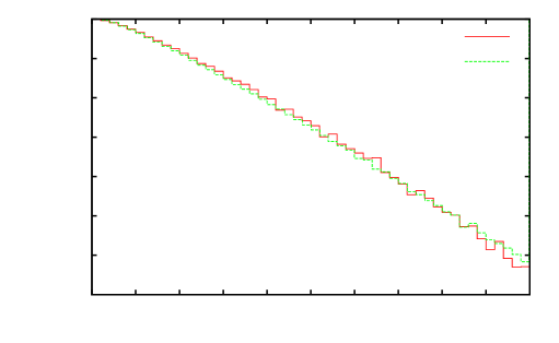
1414-141212-121010-1088-866-644-422-20000200200200400400400600600600800800800100010001000120012001200140014001400160016001600180018001800200020002000

δ[%]\delta\;[\%]

kT,1[GeV]subscript𝑘T1delimited-[]GeVk_{\mathrm{T},1}\;[\mathrm{GeV}]Refer to captionδweak1-loopsubscriptsuperscript𝛿1-loopweak\delta^{\text{1-loop}}_{\mathrm{weak}}Fig. 9 Ref. [18]
Figure 22: Comparison of the weak one-loop correction δweak1-loopsubscriptsuperscript𝛿1-loopweak\delta^{\text{1-loop}}_{\mathrm{weak}} to the transverse-momentum spectrum of the leading jet as obtained from our calculation to the result of Ref. [18].

This is confirmed in Fig. 22 which shows our result on the corrections to the transverse-momentum spectrum of the leading jet in comparison to the one shown to Fig. 9 of Ref. [18]. The two results show good agreement over the considered kT,1subscript𝑘T1k_{\mathrm{T},1} range.

We have also tried to perform a tuned comparison to the results of Ref. [17], but have not found agreement.333To find the source of discrepancy seems to require a careful comparison of individual components of the calculation. Since the correctness of our results is backed by our two calculations and the comparison to Ref. [18], we do not see a reason to await the outcome of this procedure before publication.

4 Conclusions

In this paper we have presented the calculation of the most important electroweak corrections to dijet production at the LHC and the Tevatron. These corrections comprise electroweak contributions of 𝒪(αsα,α2)𝒪subscript𝛼s𝛼superscript𝛼2{\mathcal{O}\left(\alpha_{\mathrm{s}}\alpha,\,\alpha^{2}\right)} to the LO QCD prediction as well as NLO corrections through the order αs2αsuperscriptsubscript𝛼s2𝛼\alpha_{\mathrm{s}}^{2}\alpha. Guided by the electroweak Sudakov-type logarithms induced by soft or collinear W/Z exchange at high energies, we have restricted ourselves to the calculation of the purely weak loop corrections in a first step.

For the integrated cross section with minimal cuts we find that the weak corrections are negligible, typically staying below the per-cent level, both at the LHC and the Tevatron. However, the electroweak Sudakov logarithms affect the tails of kinematic distributions that are sensitive to the high energy scales of the hard scattering process. We have discussed this feature in some detail, considering the distributions in the dijet invariant mass (M12subscript𝑀12M_{12}), and in the transverse momenta of the leading (kT,1subscript𝑘T1k_{\mathrm{T},1}) and the subleading (kT,2subscript𝑘T2k_{\mathrm{T},2}) jets.

For the s=14TeV𝑠14TeV\sqrt{s}=14\leavevmode\nobreak\ \mathrm{TeV} LHC setup, we observe weak loop corrections of 𝒪(αs2α)𝒪superscriptsubscript𝛼s2𝛼{\mathcal{O}\left(\alpha_{\mathrm{s}}^{2}\alpha\right)} reaching up to 12%percent12-12\% (16%percent16-16\%) for a transverse momentum of kT=3TeVsubscript𝑘T3TeVk_{\mathrm{T}}=3\leavevmode\nobreak\ \mathrm{TeV} of the leading (subleading) jet, whereas the dijet invariant-mass distribution only receives weak corrections up to 6%percent6-6\% for M12=6TeVsubscript𝑀126TeVM_{12}=6\leavevmode\nobreak\ \mathrm{TeV}. This difference is explained by the fact that observables based on specific ranges in M12subscript𝑀12M_{12} are not dominated by the Sudakov regime (large energies at fixed angles) for large M12subscript𝑀12M_{12} values, but rather characterized by the Regge (forward) regime. The weak corrections to dijet production at the Tevatron show similar features, though their size is smaller (10%percent10-10\% for kT=800GeVsubscript𝑘T800GeVk_{\mathrm{T}}=800\leavevmode\nobreak\ \mathrm{GeV}) than for the LHC because of the smaller scattering energy.

The LO EW contributions of 𝒪(αsα,α2)𝒪subscript𝛼s𝛼superscript𝛼2{\mathcal{O}\left(\alpha_{\mathrm{s}}\alpha,\,\alpha^{2}\right)} turn out to be of the same order of magnitude as the weak loop corrections. At the LHC, these two types of corrections partially cancel, but the degree of this cancellation depends on the chosen observable, setup, and cuts, so that the full calculation is necessary in order to correctly include the considered electroweak effects. At the Tevatron the LO electroweak corrections are somewhat smaller than the weak loop effects, but of the same sign at high transverse jet momenta, thus somewhat enhancing the electroweak effects to 12%percent12-12\% at kT=800GeVsubscript𝑘T800GeVk_{\mathrm{T}}=800\leavevmode\nobreak\ \mathrm{GeV}.

The electroweak corrections considered in this paper are supposed to be the by far dominant electroweak effects in dijet production at hadron colliders. Their numerical impact of 1020%10percent2010{-}20\% in the TeV range is not negligible and will certainly play a significant role once the NNLO QCD corrections are known. In contrast to the weak corrections, which get dominated by the large Sudakov logarithms at high energies, the so-far-neglected photonic loop corrections do not receive particular enhancements over their parametric suppression by the electromagnetic coupling α𝛼\alpha. The calculation of these effects, which are expected to stay at the few-per-cent level, are left to the future.

Acknowledgements

A.H. is supported by the German Research Foundation (DFG) via grant DI 784/2-1.

References

  • [1] R. M. Harris and K. Kousouris, Int. J. Mod. Phys. A 26 (2011) 5005 [arXiv:1110.5302 [hep-ex]].
  • [2] G. Aad et al. [ATLAS Collaboration], Phys.  Rev. D 86 (2012) 014022 [arXiv:1112.6297 [hep-ex]].
  • [3] CMS Collaboration, CMS-PAS-QCD-11-004.
  • [4] T. Aaltonen et al. [CDF Collaboration], Phys. Rev. D 78 (2008) 052006 [Erratum-ibid. D 79 (2009) 119902] [arXiv:0807.2204 [hep-ex]].
  • [5] V. M. Abazov et al. [D0 Collaboration], Phys. Rev. D 85 (2012) 052006 [arXiv:1110.3771 [hep-ex]].
  • [6] B. L. Combridge, J. Kripfganz and J. Ranft, Phys. Lett. B 70 (1977) 234.
  • [7] S. D. Ellis, Z. Kunszt and D. E. Soper, Phys. Rev. Lett.  64 (1990) 2121.
  • [8] S. D. Ellis, Z. Kunszt and D. E. Soper, Phys. Rev. Lett.  69 (1992) 1496.
  • [9] W. T. Giele, E. W. N. Glover and D. A. Kosower, Phys. Rev. Lett.  73 (1994) 2019 [hep-ph/9403347].
  • [10] T. Gehrmann, PoS DIS 2010 (2010) 004 [arXiv:1007.2107 [hep-ph]].
  • [11] A. Gehrmann-De Ridder, PoS ICHEP 2010 (2010) 106.
  • [12] P. Bolzoni, G. Somogyi and Z. Trocsanyi, JHEP 1101 (2011) 059 [arXiv:1011.1909 [hep-ph]].
  • [13] R. Boughezal, A. Gehrmann-De Ridder and M. Ritzmann, JHEP 1102 (2011) 098 [arXiv:1011.6631 [hep-ph]].
  • [14] A. Gehrmann-De Ridder, E. W. N. Glover and J. Pires, JHEP 1202 (2012) 141 [arXiv:1112.3613 [hep-ph]].
  • [15] T. Gehrmann and P. F. Monni, JHEP 1112 (2011) 049 [arXiv:1107.4037 [hep-ph]].
  • [16] A. G. -D. Ridder, T. Gehrmann and M. Ritzmann, arXiv:1207.5779 [hep-ph].
  • [17] S. Moretti, M. R. Nolten and D. A. Ross, Nucl. Phys. B 759 (2006) 50 [hep-ph/0606201].
  • [18] A. Scharf, arXiv:0910.0223 [hep-ph].
  • [19] J. H. Kühn, A. Scharf and P. Uwer, Phys. Rev. D 82 (2010) 013007 [arXiv:0909.0059 [hep-ph]].
  • [20] V. S. Fadin, L. N. Lipatov, A. D. Martin and M. Melles, Phys. Rev. D 61 (2000) 094002 [hep-ph/9910338].
  • [21] M. Ciafaloni, P. Ciafaloni and D. Comelli, Phys. Rev. Lett.  84 (2000) 4810 [hep-ph/0001142].
  • [22] M. Hori, H. Kawamura and J. Kodaira, Phys. Lett. B 491 (2000) 275 [hep-ph/0007329].
  • [23] M. Melles, Eur. Phys. J. C 24 (2002) 193 [hep-ph/0108221].
  • [24] W. Beenakker and A. Werthenbach, Nucl. Phys. B 630 (2002) 3 [hep-ph/0112030].
  • [25] A. Denner, M. Melles and S. Pozzorini, Nucl. Phys. B 662 (2003) 299 [hep-ph/0301241].
  • [26] B. Jantzen, J. H. Kühn, A. A. Penin, V. A. Smirnov, and , Phys. Rev. D 72 (2005) 051301 [Erratum-ibid. D 74 (2006) 019901] [hep-ph/0504111].
  • [27] B. Jantzen, J. H. Kühn, A. A. Penin, V. A. Smirnov and , Nucl. Phys. B 731 (2005) 188 [Erratum-ibid. B 752 (2006) 327] [hep-ph/0509157].
  • [28] U. Baur, Phys. Rev. D 75 (2007) 013005 [hep-ph/0611241].
  • [29] J. H. Kühn, A. A. Penin and V. A. Smirnov, Nucl. Phys. Proc. Suppl.  89 (2000) 94 [hep-ph/0005301].
  • [30] J. H. Kühn, A. A. Penin and V. A. Smirnov, Eur. Phys. J. C 17 (2000) 97 [hep-ph/9912503].
  • [31] S. Dittmaier and M. Krämer, Phys. Rev. D 65 (2002) 073007 [hep-ph/0109062].
  • [32] A. Denner, S. Dittmaier, M. Roth and D. Wackeroth, Nucl. Phys. B 560 (1999) 33 [hep-ph/9904472].
  • [33] A. Denner, S. Dittmaier, M. Roth and L. H. Wieders, Nucl. Phys. B 724 (2005) 247 [Erratum-ibid. B 854 (2012) 504] [hep-ph/0505042].
  • [34] S. Catani and M. H. Seymour, Nucl. Phys. B 485 (1997) 291 [Erratum-ibid. B 510 (1998) 503] [hep-ph/9605323].
  • [35] S. Catani, S. Dittmaier, M. H. Seymour and Z. Trocsanyi, Nucl. Phys. B 627 (2002) 189 [hep-ph/0201036].
  • [36] S. Dittmaier, Phys. Rev. D 59 (1998) 016007 [hep-ph/9805445].
  • [37] T. Hahn, Comput. Phys. Commun.  140 (2001) 418 [hep-ph/0012260].
  • [38] T. Hahn and M. Perez-Victoria, Comput. Phys. Commun.  118 (1999) 153 [hep-ph/9807565].
  • [39] A. Denner and S. Dittmaier, Nucl. Phys. B 734 (2006) 62 [hep-ph/0509141].
  • [40] A. Denner and S. Dittmaier, Nucl. Phys. B 844 (2011) 199 [arXiv:1005.2076 [hep-ph]].
  • [41] G. P. Lepage, CLNS-80/447.
  • [42] J. Küblbeck, M. Böhm and A. Denner, Comput. Phys. Commun.  60 (1990) 165.
  • [43] M. Moretti, T. Ohl and J. Reuter, hep-ph/0102195.
  • [44] T. Ohl, Comput. Phys. Commun.  120 (1999) 13 [hep-ph/9806432].
  • [45] G. Bell, J. H. Kühn and J. Rittinger, Eur. Phys. J. C 70 (2010) 659 [arXiv:1004.4117 [hep-ph]].
  • [46] A. Bredenstein, A. Denner, S. Dittmaier and S. Pozzorini, JHEP 0808 (2008) 108 [arXiv:0807.1248 [hep-ph]].
  • [47] A. Denner, Fortsch. Phys.  41 (1993) 307 [arXiv:0709.1075 [hep-ph]].
  • [48] T. Kinoshita, J. Math. Phys.  3 (1962) 650.
  • [49] T. D. Lee and M. Nauenberg, Phys. Rev.  133 (1964) B1549.
  • [50] C. Amsler et al. [Particle Data Group Collaboration], Phys. Lett. B 667 (2008) 1 and 2009 partial update for the 2010 edition.
  • [51] D. Y. Bardin, A. Leike, T. Riemann and M. Sachwitz, Phys. Lett. B 206 (1988) 539.
  • [52] J. Pumplin, D. R. Stump, J. Huston, H. L. Lai, P. M. Nadolsky and W. K. Tung, JHEP 0207 (2002) 012 [hep-ph/0201195].
  • [53] M. Cacciari, G. P. Salam and G. Soyez, JHEP 0804 (2008) 063 [arXiv:0802.1189 [hep-ph]].