Collider-independent top quark forward-backward asymmetries:
standard model predictions

Abstract

We compute, for top quark pair production at the Tevatron and the Large Hadron Collider, the collider-independent forward-backward asymmetries defined in AguilarSaavedra:2012va in the standard model at next-to-leading order in QCD, including also electromagnetic and weak corrections.

I Introduction

The charge asymmetry – respectively forward-backward (FB) asymmetry – in $t\bar{t}$ production at the Fermilab Tevatron stands out as perhaps the most prominent anomaly that the data analysis of this collider has left. The observable that has been mostly used is the $t\bar{t}$ rest frame asymmetry whose definition is based on the difference $\Delta y=y_{t}-y_{\bar{t}}$ between the rapidities of the top quark and antiquark, which is invariant under boosts along the beam direction,

$$A_{FB}=\frac{N(\Delta y>0)-N(\Delta y<0)}{N(\Delta y>0)+N(\Delta y<0)}\,,$$ (1)

where $N$ denotes the respective number of $t\bar{t}$ events. The measurements of this asymmetry by the CDF Aaltonen:2011kc ; CDF8.7 and D0 Abazov:2011rq Collaborations, which are in excess of the standard model (SM) expectations Kuhn:1998kw ; Antunano:2007da ; Almeida:2008ug ; Bernreuther:2010ny ; Kidonakis:2011zn ; Ahrens:2011uf ; Hollik:2011ps ; Kuhn:2011ri ; Campbell:2012uf ; Bernreuther:2012sx , have triggered more than a hundred theory papers that explain this anomaly by new physics (see, for example, Djouadi:2009nb ; Jung:2009jz ; Cheung:2009ch ; Nelson:2011us ; Shu:2009xf ; Barcelo:2011vk ). New physics explanations of the anomalous Tevatron asymmetry often predict new related effects at the Large Hadron Collider (LHC) Cao:2011ew , including the observation of new particles Gresham:2011pa . As yet, none of these effects have been found at the LHC. But, of course, this does not rule out the possibility that the Tevatron asymmetry results from new physics, telling us that, if anything, this new physics is perhaps not as simply modeled as by the hitherto existing proposals.

A closer test of the Tevatron excess is provided by the measurement of the $t\bar{t}$ charge asymmetry at the LHC. While the Tevatron FB asymmetry in Eq. (1) involves the rapidity difference $\Delta y$, the definition of the LHC charge asymmetry used by the CMS and ATLAS experiments employs the difference $\Delta|y|=|y_{t}|-|y_{\bar{t}}|$ between the absolute values of the top and anti-top rapidities in the laboratory (LAB) frame Diener:2009ee ,

$$A_{C}=\frac{N(\Delta|y|>0)-N(\Delta|y|<0)}{N(\Delta|y|>0)+N(\Delta|y|<0)}\,.$$ (2)

This definition takes advantage of the fact that valence quarks $q=u,d$ have a larger average momentum fraction than antiquarks $\bar{q}$. This leads to a boost of the $t\bar{t}$ system along the direction of the incoming quark. Therefore, an excess of top quarks in this direction – that is, a FB asymmetry in the center-of-mass (CM) frame of the initial partons – leads to more $t$ than $\bar{t}$ quarks for large values $|y|$ of the (anti)top rapidity, while for small values of $|y|$ it is the other way around. Current measurements of $A_{C}$ by the ATLAS Aad:2012ug and CMS Chatrchyan:2011hk ; Chatrchyan:2012xv Collaborations have found agreement with the SM predictions. However, these results are per se not incompatible with the Tevatron measurements AguilarSaavedra:2012va ; Drobnak:2012cz ; Alvarez:2012ca ; Drobnak:2012rb , since $A_{FB}$ and $A_{C}$ are different observables that result from a different “weighting” of the “intrinsic” asymmetries $A_{u}$, $A_{d}$ in $u\bar{u}\to t\bar{t}$, $d\bar{d}\to t\bar{t}$, respectively. (Notice that $gg\to t\bar{t}$ does not contribute to $A_{FB}$ and $A_{C}$.) In this way, models giving rise to different intrinsic asymmetries $A_{u}$, $A_{d}$, lead to different predictions for the relation between $A_{C}$ and $A_{FB}$ AguilarSaavedra:2011hz .

A direct test of the Tevatron anomaly has been proposed AguilarSaavedra:2012va that consists in the extraction of the asymmetries $A_{u,d}$ from the measurement of the suitably binned asymmetries of Eqs. (1), (2) at the Tevatron and LHC, respectively, and the subsequent comparison of the respective results. Their numerical values are nearly the same at both colliders, up to corrections that are much smaller than the experimental precision; thus their denomination as “collider-independent”. The determination of the same quantities at the two colliders could shed light on the origin of the Tevatron anomalies and settle the apparent tension with the LHC measurements.

The asymmetries $A_{u,d}$ can be extracted from the FB and charge asymmetries in Eqs. (1), (2) because they can be written, to a good approximation, as

$$A_{FB} = A_{u}F_{u}+A_{d}F_{d}\,,$$

$$A_{C} = A_{u}F_{u}D_{u}+A_{d}F_{d}D_{d}\,,$$ (3)

provided we restrict ourselves to a narrow interval in the $t\bar{t}$ invariant mass $m_{t\bar{t}}$. This will be shown below. The factors $F_{q}$ – which differ at Tevatron and the LHC and also depend on the CM energy – can be interpreted at leading order QCD as the fractions of $q\bar{q}$ initiated $t\bar{t}$ events. The $D_{q}$ are “dilution” factors that take into account that in $t\bar{t}$ production at the LHC it often happens that the initial valence quark has smaller momentum fraction than the sea antiquark, thus leading to a dilution of the asymmetry generated at the partonic level. Both $F_{q}$ and $D_{q}$ depend on the longitudinal velocity of the $t\bar{t}$ pair in the LAB frame,

$$\beta=\frac{|p_{t}^{z}+p_{\bar{t}}^{z}|}{E_{t}+E_{\bar{t}}}\,,$$ (4)

where $E$, $p^{z}$ are the LAB-frame (anti)top energy and momentum along the beam direction, respectively. On the other hand, for fixed $\hat{s}$, $A_{u,d}$ are $\beta$-independent. In practice, where a finite $m_{t\bar{t}}$ interval has to be used instead of $\hat{s}$, $A_{u,d}$ become mildly $\beta$-dependent. This $\beta$-dependence can be weakened by imposing an upper cut on the transverse momentum $p_{T}^{t\bar{t}}$ of the $t\bar{t}$ pair. Hence, for a chosen interval $m_{L}<m_{t\bar{t}}<m_{U}$, $A_{u,d}$ can be extracted from a fit to the distributions $A_{FB}(\beta)$ and $A_{C}(\beta)$ measured within this $m_{t\bar{t}}$ interval, as discussed in AguilarSaavedra:2012va , using the $F_{q}$ and $D_{q}$ factors computed in the SM, e.g. by Monte Carlo.

In this paper we calculate $A_{u,d}$ in the SM at next-to-leading order (NLO) in the QCD coupling, including also electromagnetic and weak corrections. To be precise, “NLO” refers in this paper to the computation of the numerators in Eqs. (1), (2) to order $\alpha_{s}^{3}$ including the electroweak corrections of order $\alpha_{s}^{2}\alpha$. In the next section we derive Eqs. (3) in detail for the SM at NLO. This derivation holds also if there are new physics contributions to the asymmetries (1), (2). In addition, we discuss the role of $gq$ contributions, which also lead to an asymmetry at the LHC, albeit very small in the SM. In section III we present our numerical results.

II Derivations

The following derivations apply to the computation of the numerators of Eqs. (1), (2) to NLO in the gauge couplings (see above). These numerators receive non-zero contributions only from terms in the squared matrix elements that are asymmetric with respect to the exchange of the $t$ and $\bar{t}$ momenta. As it is well-known, respective contributions $d\sigma^{A}$ only arise from the matrix elements of $q\bar{q}\to t\bar{t}(g,\gamma)$, where $q=u,d$, and of $gq(\bar{q})\to t\bar{t}q(\bar{q})$. To NLO in the gauge couplings, the charge asymmetric terms $d\sigma^{A}_{qg}$ are infrared-finite, while for $q\bar{q}$ initiated $t\bar{t}$ production, the soft-gluon divergence that is present in $d\sigma^{A}_{q\bar{q}}$ (virtual + soft) cancels against the corresponding divergence in $\int d\sigma^{A}_{q\bar{q}}$ ($t{\bar{t}}g),$ and likewise for real photon radiation. To NLO in the gauge couplings, the numerators of Eqs. (1), (2) are free of initial-state collinear singularities – i.e., no collinear counterterms are required to this order.

The NLO numerators are denoted by $N^{1}$ in the following. For definiteness, we consider the denominators of Eqs. (1), (2) to leading order (LO) and denote them by $N^{0}$. Yet, alternatively, NLO denominators may be used, and the derivations are completely analogous to the ones presented here. Quantities without subindices imply a sum over all partonic sub-processes, whereas a subindex, if present, indicates the corresponding subprocess. For brevity we label with superscripts $F,B$ the $t\bar{t}$ events with $\Delta y\gtrless 0$, respectively, and with superscripts $>,<$ the events with $\Delta|y|\gtrless 0$.

To NLO, the numerator of Eq. (1) receives contributions from $q{\bar{q}}\to t{\bar{t}}(g,\gamma)$, $q=u,d$. Top-quark pair production by $gg$ fusion is symmetric, and contributions to the numerator of Eq. (1) by $qg$, ${\bar{q}}g$ processes are completely negligible at the Tevatron. Then, the FB asymmetry takes the form

$$A_{FB} = \frac{N_{u\bar{u}}^{1,F}-N_{u\bar{u}}^{1,B}}{N^{0}}+(u\to d)$$ (5)

$$= \frac{N_{u\bar{u}}^{1,F}-N_{u\bar{u}}^{1,B}}{N_{u\bar{u}}^{0}}\frac{N_{u\bar{u}}^{0}}{N^{0}}+(u\to d)$$

$$\equiv A_{u}F_{u}+A_{d}F_{d}\,.$$

Likewise, the LHC charge asymmetry in Eq. (2) can be written as

$$A_{C} = \frac{N_{u\bar{u}}^{1,>}-N_{u\bar{u}}^{1,<}}{N^{0}}+\frac{N_{gu}^{1,>}-N_{gu}^{1,<}}{N^{0}}+(u\to d)$$ (6)

$$= \frac{N_{u\bar{u}}^{1,>}-N_{u\bar{u}}^{1,<}}{N_{u\bar{u}}^{0}}\frac{N_{u\bar{u}}^{0}}{N^{0}}+\frac{N_{gu}^{1,>}-N_{gu}^{1,<}}{N_{u\bar{u}}^{0}}\frac{N_{u\bar{u}}^{0}}{N^{0}}$$

$$+(u\to d)\,.$$

The denominators $N^{0}$ in Eqs. (5) and (6) are the (binned) LO QCD $t\bar{t}$ cross sections at the Tevatron and LHC, respectively. For ease of notation, we use the symbols $N^{0}$, $N_{q\bar{q}}^{1,F}$, etc., both for the Tevatron and the LHC. The SM contributions to the numerator of the charge asymmetry from $gq$ sub-processes are rather small Kuhn:2011ri ; Bernreuther:2012sx and can be ignored. (We will explicitly compute them in the next section.) Moreover, it will be shown below that, provided we restrict ourselves to a narrow $\hat{s}$ interval and to small values of $p_{T}^{t\bar{t}}$, the differences $N_{q\bar{q}}^{1,>}-N_{q\bar{q}}^{1,<}$ are related to the differences $N_{q\bar{q}}^{1,F}-N_{q\bar{q}}^{1,B}$ (where “forward” and “backward” refer to the initial quark direction) by

$$N_{q\bar{q}}^{1,>}-N_{q\bar{q}}^{1,<}=D_{q}\left(N_{q\bar{q}}^{1,F}-N_{q\bar{q}}^{1,B}\right)\,.$$ (7)

Here $D_{q}$ is a so-called dilution factor, defined, again for a narrow interval in $\hat{s}$, by

$$D_{q}\equiv\frac{N(x_{q}>x_{\bar{q}})-N(x_{q}<x_{\bar{q}})}{N(x_{q}>x_{\bar{q}})+N(x_{q}<x_{\bar{q}})}\,.$$ (8)

Using Eq. (7) and neglecting the $gq$ contributions, the charge asymmetry (6) can be written as

$$A_{C} = \frac{N_{u\bar{u}}^{1,>}-N_{u\bar{u}}^{1,<}}{N_{u\bar{u}}^{0}}\frac{N_{u\bar{u}}^{0}}{N^{0}}+(u\to d)$$ (9)

$$= \frac{N_{u\bar{u}}^{1,F}-N_{u\bar{u}}^{1,B}}{N_{u\bar{u}}^{0}}\frac{N_{u\bar{u}}^{0}}{N^{0}}D_{u}+(u\to d)$$

$$\equiv A^{\prime}_{u}F^{\prime}_{u}D_{u}+A^{\prime}_{d}F^{\prime}_{d}D_{d}\,.$$

Here, we have put primes on $A^{\prime}_{q}$ and $F^{\prime}_{q}$ to emphasize that these quantities correspond to the LHC, while the unprimed quantities refer to the Tevatron. However, as it will be shown below, the asymmetries $A^{\prime}_{u,d}$ are, for the same narrow interval in $\hat{s}$, approximately equal to the Tevatron asymmetries $A_{u,d}$ defined in Eq. (5).

We will first show the equality between $A_{u,d}$ and $A_{u,d}^{\prime}$. For the latter, the forward and backward directions are defined with respect to the initial quark momentum direction. (Of course this is impossible to tell event by event.) Then, we derive Eq. (7). Our notation is as follows. We denote by $x_{i}$, $i=1,2$ the momentum fractions of the initial partons, and $f_{p}(x_{i})$ is the distribution function for parton $p$ in the proton with momentum fraction $x_{i}$. The dependence of the parton distribution functions (PDF) on the factorization scale $\mu_{F}$ is not exhibited. The (anti)proton 4-momenta at the Tevatron and LHC, respectively, are denoted by $P_{1,2}$, and $d\hat{\sigma}$ denotes the differential cross section of a partonic subprocess which includes the corresponding phase-space measure $d\Phi$ and flux factor.

In the following, we consider binned asymmetries by restricting the partonic CM energy $\hat{s}$ to an interval $[\hat{s}_{\text{min}},\hat{s}_{\text{max}}]$. This is accomplished by a factor

$$\mathcal{H}=\theta(\hat{s}-\hat{s}_{\text{min}})\theta(\hat{s}_{\text{max}}-\hat{s})$$ (10)

in the integrals.

At the Tevatron, the FB asymmetries $A_{u,d}$ are defined with respect to the proton direction. Their numerators are, in terms of the proton PDF,

$$N_{q\bar{q}}^{1,F}-N_{q\bar{q}}^{1,B} = \int dx_{1}dx_{2}\,f_{q}(x_{1})f_{q}(x_{2})d\hat{\sigma}^{1}[q(x_{1}P_{1})\bar{q}(x_{2}P_{2})]\left[\theta(\Delta y)-\theta(-\Delta y)\right]\mathcal{H}$$ (11)

$$+\int dx_{1}dx_{2}\,f_{\bar{q}}(x_{1})f_{\bar{q}}(x_{2})d\hat{\sigma}^{1}[q(x_{2}P_{2})\bar{q}(x_{1}P_{1})]\left[\theta(\Delta y)-\theta(-\Delta y)\right]\mathcal{H}\,,$$

where $d{\hat{\sigma}}^{1}$ denotes here the sum of the $q\bar{q}$ initiated NLO differential cross sections for 2-particle and 3-particle final states, and $\Delta y$ is the difference of the $t$ and $\bar{t}$ rapidities in the CM frame of the initial partons. The second integral corresponds to events where the initial anti-quark comes from the proton and the quark from the anti-proton, and is much smaller than the first integral. (It amounts to a “dilution” of order $10^{-3}$ in the asymmetry.) Choosing $\hat{s}_{\text{max}}$ and $\hat{s}_{\text{min}}$ in (10) close enough to each other, the factor $\mathcal{H}$ fixes $\hat{s}$ within a suitably narrow interval, in which $\int d\hat{\sigma}^{1}$, which are functions of $\hat{s}$, are nearly constant and can then be taken out of the $x_{i}$ integrals. Dropping the argument in $d\hat{\sigma}^{1}$ for brevity,

$$N_{q\bar{q}}^{1,F}-N_{q\bar{q}}^{1,B} = \int d\hat{\sigma}^{1}[\theta(\Delta y)-\theta(-\Delta y)]$$ (12)

$$\times\int dx_{1}dx_{2}\,f_{q}(x_{1})f_{q}(x_{2})\mathcal{H}\,.$$

Notice that $\Delta y$ is independent of $x_{1}$ and $x_{2}$. The same can be done for the LO denominators,

$$N_{q\bar{q}}^{0,F}+N_{q\bar{q}}^{0,B}=\int d\hat{\sigma}^{0}_{q\bar{q}}\int dx_{i}\,f_{q}(x_{1})f_{q}(x_{2})\mathcal{H}\,,$$ (13)

where $d\sigma^{0}_{q\bar{q}}$ is the LO differential cross section for $q\bar{q}\to t\bar{t}$, so the asymmetries are

$$A_{q}=\frac{\int d\hat{\sigma}^{1}\left[\theta(\Delta y)-\theta(-\Delta y)\right]}{\int d\hat{\sigma}^{0}_{q\bar{q}}}\,.$$ (14)

The numerators of the LHC “FB” asymmetries $A^{\prime}_{u}$, $A^{\prime}_{d}$ defined in (9) are

$$N_{q\bar{q}}^{1,F}-N_{q\bar{q}}^{1,B} = \int dx_{1}dx_{2}\,f_{q}(x_{1})f_{\bar{q}}(x_{2})d\hat{\sigma}^{1}[q(x_{1}P_{1})\bar{q}(x_{2}P_{2})]\left[\theta(\Delta y)-\theta(-\Delta y)\right]\mathcal{H}$$ (15)

$$+\int dx_{1}dx_{2}\,f_{\bar{q}}(x_{1})f_{q}(x_{2})d\hat{\sigma}^{1}[q(x_{2}P_{2})\bar{q}(x_{1}P_{1})]\left[\theta(-\Delta y)-\theta(\Delta y)\right]\mathcal{H}\,,$$

where the “forward” and “backward” directions are defined with respect to the incoming quark direction (note the opposite signs in the arguments of the $\theta$ functions of the second integral). By rotational invariance, the second term is equal to the first one, so we can concentrate on the former. Taking again the phase-space integrated partonic cross sections out of the $x_{i}$ integrals, we have

$${\textstyle\frac{1}{2}}\left(N_{q\bar{q}}^{1,F}-N_{q\bar{q}}^{1,B}\right) = \int d\hat{\sigma}^{1}\left[\theta(\Delta y)-\theta(-\Delta y)\right]$$

$$\times\int dx_{1}dx_{2}\,f_{q}(x_{1})f_{\bar{q}}(x_{2})\mathcal{H}\,.$$

The LO denominators $N^{0}_{q\bar{q}}=N^{0,F}_{q\bar{q}}+N^{0,B}_{q\bar{q}}$ of $A^{\prime}_{u,d}$ are

$${\textstyle\frac{1}{2}}\left(N^{0,F}_{q\bar{q}}+N^{0,B}_{q\bar{q}}\right) = \int d\hat{\sigma}^{0}_{q\bar{q}}$$

$$\times\int dx_{1}dx_{2}\,f_{q}(x_{1})f_{\bar{q}}(x_{2})\mathcal{H}\,.$$

Thus the LHC asymmetries $A^{\prime}_{u,d}$ are, given for fixed $\hat{s}$, by

$$A^{\prime}_{q}=\frac{\int d\hat{\sigma}^{1}\left[\theta(\Delta y)-\theta(-\Delta y)\right]}{\int d\hat{\sigma}^{0}_{q\bar{q}}}\,.$$ (18)

They are equal to the ones at the Tevatron, Eq. (14).

Next we show under which conditions Eq. (7) holds. The contribution from $q\bar{q}$ initial states to the numerator of the binned LHC charge asymmetry (6) is

$$N_{q\bar{q}}^{1,>}-N_{q\bar{q}}^{1,<} = \int dx_{1}dx_{2}\,f_{q}(x_{1})f_{\bar{q}}(x_{2})d\hat{\sigma}^{1}[q(x_{1}P_{1})\bar{q}(x_{2}P_{2})]\mathcal{H}\mathcal{E}$$ (19)

$$+\int dx_{1}dx_{2}\,f_{\bar{q}}(x_{1})f_{q}(x_{2})d\hat{\sigma}^{1}[q(x_{2}P_{2})\bar{q}(x_{1}P_{1})]\mathcal{H}\mathcal{E}\,,$$

where the asymmetric terms are selected by the factor

$$\mathcal{E}=\theta(|y_{t}|-|y_{\bar{t}}|)-\theta(|y_{\bar{t}}|-|y_{t}|)\,.$$ (20)

Here $y_{t}$, $y_{\bar{t}}$ are the top and anti-top rapidities in the laboratory (LAB) frame, respectively. Using rotational invariance, the first integral equals the second one, so we can concentrate on the former. We now perform a rotation-free boost to the $t\bar{t}$ rest frame. Using that the sign of the difference of the $t$ and $\bar{t}$ rapidities is frame invariant, we obtain, with some algebra, that in the limit of $p_{T}^{t\bar{t}}\to 0$,

$$\mathcal{E}\to[\theta(x_{1}-x_{2})-\theta(x_{2}-x_{1})][\theta(\Delta y)-\theta(-\Delta y)]\,.$$ (21)

Inserting Eq. (21) into Eq. (19) we obtain that for $t\bar{t}$ events with sufficiently small $p_{T}^{t\bar{t}}$,

$${\textstyle\frac{1}{2}}(N_{q\bar{q}}^{1,>}-N_{q\bar{q}}^{1,<}) = \int dx_{1}dx_{2}\,f_{q}(x_{1})f_{\bar{q}}(x_{2})\times\left\{\theta(x_{1}-x_{2})\theta(\Delta y)-\theta(x_{1}-x_{2})\theta(-\Delta y)-\theta(x_{2}-x_{1})\theta(\Delta y)\right.$$ (22)

$$\left.+\theta(x_{2}-x_{1})\theta(-\Delta y)\right\}\times d\hat{\sigma}^{1}\mathcal{H}\,.$$

Again, the factor $\mathcal{H}$ fixes $\hat{s}$ within a suitably narrow interval, in which the $\int d\hat{\sigma}^{1}$ are nearly constant and can be taken out of the $x_{i}$ integrals:

$${\textstyle\frac{1}{2}}(N_{q\bar{q}}^{1,>}-N_{q\bar{q}}^{1,<}) = \int d\hat{\sigma}^{1}\theta(\Delta y)\int dx_{1}dx_{2}\,f_{q}(x_{1})f_{\bar{q}}(x_{2})\theta(x_{1}-x_{2})\mathcal{H}$$ (23)

$$-\int d\hat{\sigma}^{1}\theta(-\Delta y)\int dx_{1}dx_{2}\,f_{q}(x_{1})f_{\bar{q}}(x_{2})\theta(x_{1}-x_{2})\mathcal{H}$$

$$-\int d\hat{\sigma}^{1}\theta(\Delta y)\int dx_{1}dx_{2}\,f_{q}(x_{1})f_{\bar{q}}(x_{2})\theta(x_{2}-x_{1})\mathcal{H}$$

$$+\int d\hat{\sigma}^{1}\theta(-\Delta y)\int dx_{1}dx_{2}\,f_{q}(x_{1})f_{\bar{q}}(x_{2})\theta(x_{2}-x_{1})\mathcal{H}\,.$$

Now let us define

$$d_{q}^{r} \equiv \frac{\int dx_{1}dx_{2}\,f_{q}(x_{1})f_{\bar{q}}(x_{2})d\hat{\sigma}_{q\bar{q}}\theta(x_{1}-x_{2})\mathcal{H}}{\int dx_{1}dx_{2}\,f_{q}(x_{1})f_{\bar{q}}(x_{2})d\hat{\sigma}_{q\bar{q}}\mathcal{H}}$$

$$= \frac{\int dx_{1}dx_{2}\,f_{q}(x_{1})f_{\bar{q}}(x_{2})\theta(x_{1}-x_{2})\mathcal{H}}{\int dx_{1}dx_{2}\,f_{q}(x_{1})f_{\bar{q}}(x_{2})\mathcal{H}}\,,$$

$$d_{q}^{w} \equiv \frac{\int dx_{1}dx_{2}\,f_{q}(x_{1})f_{\bar{q}}(x_{2})d\hat{\sigma}_{q\bar{q}}\theta(x_{2}-x_{1})\mathcal{H}}{\int dx_{1}dx_{2}\,f_{q}(x_{1})f_{\bar{q}}(x_{2})d\hat{\sigma}_{q\bar{q}}\mathcal{H}}$$ (24)

$$= \frac{\int dx_{1}dx_{2}\,f_{q}(x_{1})f_{\bar{q}}(x_{2})\theta(x_{2}-x_{1})\mathcal{H}}{\int dx_{1}dx_{2}f_{q}(x_{1})f_{\bar{q}}(x_{2})\mathcal{H}}\,.$$

Here $d\hat{\sigma}_{q\bar{q}}$ denotes the (LO or NLO) differential cross section for $q{\bar{q}}\to t\bar{t}X$. In the next section, we use $d\hat{\sigma}^{0}_{q\bar{q}}$ in (24). The cancellation of the $d\hat{\sigma}_{q\bar{q}}$ in the ratios (24) works, for fixed $\hat{s}$, also to NLO, because all the terms in $d\hat{\sigma}^{1}_{q\bar{q}}$, which is the sum of the contributions from the tree-level term, virtual corrections, soft and hard gluon radiation, and the collinear counterterm, are convoluted with the same product of PDF.

Clearly, $d_{q}^{r}+d_{q}^{w}=1$. The integrals with respect to $x_{i}$ in Eq. (23) can be written in terms of $d_{q}^{r}$ and $d_{q}^{w}$, resulting in

$${\textstyle\frac{1}{2}}(N_{q\bar{q}}^{1,>}-N_{q\bar{q}}^{1,<}) = \int d\hat{\sigma}^{1}\theta(\Delta y)\;d_{q}^{r}\int dx_{1}dx_{2}f_{q}(x_{1})f_{\bar{q}}(x_{2})\mathcal{H}-\int d\hat{\sigma}^{1}\theta(-\Delta y)\;d_{q}^{r}\int dx_{1}dx_{2}f_{q}(x_{1})f_{\bar{q}}(x_{2})\mathcal{H}$$ (25)

$$-\int d\hat{\sigma}^{1}\theta(\Delta y)\;d_{q}^{w}\int dx_{1}dx_{2}f_{q}(x_{1})f_{\bar{q}}(x_{2})\mathcal{H}+\int d\hat{\sigma}^{1}\theta(-\Delta y)\;d_{q}^{w}\int dx_{1}dx_{2}f_{q}(x_{1})f_{\bar{q}}(x_{2})\mathcal{H}\,.$$

Rearranging terms, we have

$${\textstyle\frac{1}{2}}(N_{q\bar{q}}^{1,>}-N_{q\bar{q}}^{1,<}) = (d_{q}^{r}-d_{q}^{w})\int dx_{1}dx_{2}\,f_{q}(x_{1})f_{\bar{q}}(x_{2})$$ (26)

$$\times d\hat{\sigma}^{1}[\theta(\Delta y)-\theta(-\Delta y)]\mathcal{H}\,.$$

Comparing with Eq. (LABEL:ec:NlhcFB) we obtain Eq. (7), i.e.,

$$N_{q\bar{q}}^{1,>}-N_{q\bar{q}}^{1,<}=(d_{q}^{r}-d_{q}^{w})\left(N_{q\bar{q}}^{1,F}-N_{q\bar{q}}^{1,B}\right)\,,$$ (27)

where

$$d_{q}^{r}-d_{q}^{w}=D_{q}$$ (28)

are the dilution factors introduced in Eqs. (7), (8).

We recall that this derivation holds for fixed $\hat{s}$ and sufficiently small $p_{T}^{t\bar{t}}$. On the other hand, the formula (27) and the resulting formula (9) holds for arbitrary values $0<\beta<1$ of the longitudinal velocity of the $t\bar{t}$ system. In practice, the requirement of fixed $\hat{s}$ must be replaced by choosing a reasonably narrow bin in the $t\bar{t}$ invariant mass $m_{t\bar{t}}$, i.e.,

$$\mathcal{H}\longrightarrow\theta(m_{t\bar{t}}-m_{L})\theta(m_{U}-m_{t\bar{t}})\,.$$ (29)

This will be done in the numerical computations of the next section. Then the intrinsic asymmetries $A^{\mbox{\tiny(${}^{\prime}$)}}_{u,d}$ will become $\beta$-dependent; that is, the formulae Eqs. (14) and (18) do no longer apply – for the computations one has to use instead the definitions of $A^{\mbox{\tiny(${}^{\prime}$)}}_{u,d}$ given in Eqs. (5) and (9), respectively. But we will show that, for a given $m_{t\bar{t}}$ bin, this $\beta$-dependence is rather mild in the SM to NLO. More importantly, as the results below will signify, $A^{\prime}_{u}$ and $A^{\prime}_{d}$ remain equal to $A_{u}$ and $A_{d}$, respectively, to a good approximation – even if no upper cut is imposed on $p_{T}^{t\bar{t}}$. In addition we will show by numerical computation that neglecting the $gq$ contributions to the LHC charge asymmetry $A_{C}$ in the formula (6) is indeed justified, given the level of precision one aims at in applying Eq.(6) to future data analysis.

III Numerical results

Our numerical calculations are based on the code described in Bernreuther:2010ny ; Bernreuther:2012sx . We compute the binned asymmetries of Eqs. (1) and (2), and the asymmetries $A_{u,d}$ (Tevatron) and $A^{\prime}_{u,d}$ (LHC, 7 and 8 TeV) for a sequence of intervals $m_{L}<m_{t\bar{t}}<m_{U}$. Within a specified interval $[m_{L},m_{U}]$, the asymmetries $A_{FB}$ and $A_{C}$ are computed, for $\beta$ bins of width $\Delta\beta$ = 0.2 for the Tevatron (i.e., $0<\beta<0.2$, etc.) and $\Delta\beta$ = 0.1 for the LHC (i.e., $0<\beta<0.1$, etc.).

In the numerators of Eqs. (1) and (2) and of $A{\mbox{\tiny(${}^{\prime}$)}}_{u,d}$ we take into account the ${\cal O}(\alpha_{s}^{3})$ QCD and the ${\cal O}(\alpha_{s}^{2}\alpha)$ electroweak corrections. For definiteness, we evaluate the denominators of all asymmetries considered in this paper with LO QCD matrix elements, which is in the spirit of a consistent fixed-order perturbative expansion of ratios like Eqs. (1), (2). The fractions $F^{\mbox{\tiny(${}^{\prime}$)}}_{q}$ and the dilution factors $D_{q}$ are computed for the Tevatron and the LHC (7 and 8 TeV) using LO QCD matrix elements both in the numerators and denominators. We evaluate both the numerators and denominators of the binned asymmetries and of $F^{\mbox{\tiny(${}^{\prime}$)}}_{q}$ and $D_{q}$ with NLO parton distribution functions.

As emphasized above, the analysis for $A^{\mbox{\tiny(${}^{\prime}$)}}_{u,d}$ could also be done by replacing, on the left- and right-hand sides of Eqs. (5) and (6), the global normalization factors $N^{0}$ (Tevatron and LHC) by the respective NLO factors $N^{1}$.

We use $m_{t}=173.1$ GeV (on-shell mass), the QED coupling $\alpha(m_{Z})=0.008$, and the weak mixing angle $\sin^{2}\theta_{W}=0.23$. We use the CTEQ6.6M PDF Nadolsky:2008zw and the respective value of $\alpha_{s}(m_{Z})$ provided by this set. We put $\mu_{R}=\mu_{F}=\mu$, and numerical results are given for $\mu=m_{t}/2,m_{t}$, and $2m_{t}$. These scale choices are purely conventional. In Ref. AguilarSaavedra:2012va the asymmetries $A^{\mbox{\tiny(${}^{\prime}$)}}_{u,d}$ were obtained for a benchmark new physics model using a two-parameter fit to the $A_{FB}(\beta)$ and $A_{C}(\beta)$ distributions, mimicking the procedure that has to be eventually performed with real data. That can be done, for the Tevatron and the LHC, by minimizing

$$\chi^{2} = \sum_{i}\frac{\left[A_{FB}(\beta_{i})-A_{u}\;F_{u}(\beta_{i})-A_{d}\;F_{d}(\beta_{i})\right]^{2}}{\left[dA_{FB}(\beta_{i})\right]^{2}}\,,$$

$$\chi^{2} = \sum_{i}\frac{\left[A_{C}(\beta_{i})-A^{\prime}_{u}\;F^{\prime}_{u}D_{u}(\beta_{i})-A^{\prime}_{d}\;F^{\prime}_{d}D_{d}(\beta_{i})\right]^{2}}{\left[dA_{C}(\beta_{i})\right]^{2}}\,,$$

with respect to $A^{\mbox{\tiny(${}^{\prime}$)}}_{u}$ and $A^{\mbox{\tiny(${}^{\prime}$)}}_{d}$. Here $i$ labels the different $\beta$ bins and $dA_{FB}(\beta_{i})$, $dA_{C}(\beta_{i})$ are the statistical uncertainties of the binned asymmetries. Unfortunately, this procedure requires extremely high Monte Carlo statistics in order to have the two-parameter fit converging to the true values. Especially at the LHC, the $\beta$-binned $A^{\prime}_{u,d}$ are obtained from the ratio of a tiny asymmetry $A_{C}(\beta_{i})$ over a small $F_{q}D_{q}(\beta_{i})$ factor. Therefore, in order to save computing time, we calculate the asymmetries with a one-parameter fit, considering $u\bar{u}$ and $d\bar{d}$ contributions separately. The values of $A^{\mbox{\tiny(${}^{\prime}$)}}_{u,d}$ presented in Tables 1 - 3 below are obtained from a one-dimensional least squares parameter fit,

$$A_{q} = \sum_{i}\frac{A_{FB}^{q\bar{q}}(\beta_{i})}{\left[dA_{FB}^{q\bar{q}}(\beta_{i})\right]^{2}}\left/\sum_{i}\frac{1}{\left[dA_{FB}^{q\bar{q}}(\beta_{i})\right]^{2}}\right.\,,$$

$$A^{\prime}_{q} = \sum_{i}\frac{A_{C}^{q\bar{q}}(\beta_{i})/D_{q}(\beta_{i})}{\left[dA_{C}^{q\bar{q}}(\beta_{i})\right]^{2}}\left/\sum_{i}\frac{1}{\left[dA_{C}^{q\bar{q}}(\beta_{i})\right]^{2}}\right.\,,$$ (31)

where the superscripts of $A_{FB}$, $A_{C}$ indicate that we restrict the calculation to these specific sub-processes, eventually including $gq$ contributions as well. We will demonstrate below the consistency of both methods by showing that the values of $A^{\mbox{\tiny(${}^{\prime}$)}}_{u,d}$ calculated using either (LABEL:twofit) or (31) agree very well within the expected experimental uncertainties. The one-parameter fit is more precise.

We estimate the statistical uncertainty of the $\beta$-binned asymmetries by taking an integrated luminosity of 20 fb^-1 for the Tevatron and 10 (30) fb^-1 for the LHC with 7 (8) TeV. This corresponds to an eventual combination of results from both experiments at the Tevatron and LHC, respectively. A selection efficiency of $\sim 25\%$ is taken for the semileptonic $t\bar{t}$ decay channels, similar to that found in the experimental analyses Aad:2012ug ; Chatrchyan:2011hk . This results in a combined efficiency factor of about 7%. The results for the Tevatron are collected in Table 1 and for the LHC in Tables 2 and 3, without and with an upper cut $p_{T}^{t\bar{t}}<30$ GeV.

Table 1: Asymmetries $A_{u,d}$ at the Tevatron, without $p_{T}^{t\bar{t}}$ cut (top) and for $p_{T}^{t\bar{t}}<30$ GeV (bottom).

	$\mu=m_{t}$		$\mu=2m_{t}$		$\mu=m_{t}/2$
$m_{t\bar{t}}$ [GeV]	$A_{u}$	$A_{d}$	$A_{u}$	$A_{d}$	$A_{u}$	$A_{d}$
$<400$	0.058	0.039	0.054	0.036	0.061	0.044
$400-450$	0.096	0.066	0.091	0.060	0.102	0.073
$450-500$	0.123	0.086	0.116	0.079	0.131	0.095
$500-550$	0.145	0.102	0.137	0.092	0.154	0.113
$550-600$	0.164	0.115	0.156	0.106	0.176	0.128

	$\mu=m_{t}$		$\mu=2m_{t}$		$\mu=m_{t}/2$
$m_{t\bar{t}}$ [GeV]	$A_{u}$	$A_{d}$	$A_{u}$	$A_{d}$	$A_{u}$	$A_{d}$
$<400$	0.069	0.046	0.065	0.042	0.075	0.051
$400-450$	0.117	0.078	0.110	0.071	0.126	0.087
$450-500$	0.150	0.101	0.141	0.092	0.161	0.113
$500-550$	0.178	0.120	0.167	0.109	0.191	0.135
$550-600$	0.201	0.137	0.190	0.125	0.217	0.153

Table 2: Asymmetries $A^{\prime}_{u,d}$ at the LHC (7 TeV), without $p_{T}^{t\bar{t}}$ cut (top) and for $p_{T}^{t\bar{t}}<30$ GeV (bottom).

	$\mu=m_{t}$		$\mu=2m_{t}$		$\mu=m_{t}/2$
$m_{t\bar{t}}$ [GeV]	$A^{\prime}_{u}$	$A^{\prime}_{d}$	$A^{\prime}_{u}$	$A^{\prime}_{d}$	$A^{\prime}_{u}$	$A^{\prime}_{d}$
$<400$	0.055	0.038	0.052	0.035	0.059	0.042
$400-450$	0.089	0.060	0.084	0.055	0.096	0.066
$450-500$	0.112	0.077	0.106	0.070	0.120	0.085
$500-550$	0.128	0.083	0.120	0.076	0.136	0.092
$550-600$	0.142	0.093	0.134	0.085	0.151	0.101
$600-650$	0.155	0.103	0.146	0.093	0.165	0.113
$650-700$	0.164	0.110	0.156	0.102	0.177	0.122
$700-750$	0.176	0.119	0.165	0.104	0.185	0.129
$750-800$	0.182	0.118	0.170	0.107	0.195	0.131

	$\mu=m_{t}$		$\mu=2m_{t}$		$\mu=m_{t}/2$
$m_{t\bar{t}}$ [GeV]	$A^{\prime}_{u}$	$A^{\prime}_{d}$	$A^{\prime}_{u}$	$A^{\prime}_{d}$	$A^{\prime}_{u}$	$A^{\prime}_{d}$
$<400$	0.071	0.054	0.068	0.047	0.077	0.059
$400-450$	0.115	0.078	0.108	0.071	0.124	0.087
$450-500$	0.149	0.103	0.140	0.093	0.160	0.114
$500-550$	0.170	0.110	0.159	0.100	0.183	0.124
$550-600$	0.193	0.128	0.180	0.116	0.209	0.144
$600-650$	0.211	0.143	0.197	0.127	0.227	0.159
$650-700$	0.229	0.153	0.215	0.140	0.247	0.169
$700-750$	0.245	0.165	0.228	0.148	0.261	0.184
$750-800$	0.262	0.177	0.244	0.158	0.282	0.194

Table 3: Asymmetries $A^{\prime}_{u,d}$ at the LHC (8 TeV), without $p_{T}^{t\bar{t}}$ cut (top) and for $p_{T}^{t\bar{t}}<30$ GeV (bottom).

$m_{t\bar{t}}$ [GeV]	$\mu=m_{t}$		$\mu=2m_{t}$		$\mu=m_{t}/2$
	$A^{\prime}_{u}$	$A^{\prime}_{d}$	$A^{\prime}_{u}$	$A^{\prime}_{d}$	$A^{\prime}_{u}$	$A^{\prime}_{d}$
$<400$	0.055	0.038	0.052	0.035	0.059	0.042
$400-450$	0.088	0.058	0.083	0.053	0.094	0.065
$450-500$	0.111	0.075	0.105	0.070	0.118	0.084
$500-550$	0.126	0.081	0.119	0.075	0.135	0.091
$550-600$	0.139	0.089	0.131	0.081	0.147	0.097
$600-650$	0.153	0.102	0.144	0.094	0.163	0.113
$650-700$	0.161	0.107	0.153	0.099	0.172	0.120
$700-750$	0.172	0.115	0.162	0.106	0.185	0.129
$750-800$	0.177	0.115	0.167	0.106	0.190	0.131

	$\mu=m_{t}$		$\mu=2m_{t}$		$\mu=m_{t}/2$
$m_{t\bar{t}}$ [GeV]	$A^{\prime}_{u}$	$A^{\prime}_{d}$	$A^{\prime}_{u}$	$A^{\prime}_{d}$	$A^{\prime}_{u}$	$A^{\prime}_{d}$
$<400$	0.073	0.040	0.068	0.050	0.078	0.061
$400-450$	0.115	0.074	0.108	0.070	0.123	0.086
$450-500$	0.147	0.101	0.139	0.092	0.159	0.113
$500-550$	0.170	0.118	0.159	0.102	0.183	0.124
$550-600$	0.191	0.128	0.179	0.113	0.205	0.141
$600-650$	0.209	0.148	0.197	0.126	0.227	0.157
$650-700$	0.229	0.157	0.215	0.139	0.246	0.168
$700-750$	0.242	0.164	0.225	0.147	0.261	0.186
$750-800$	0.258	0.174	0.243	0.155	0.277	0.193

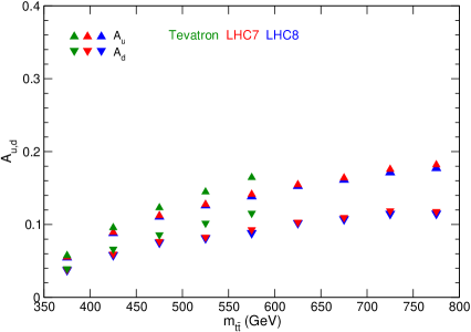
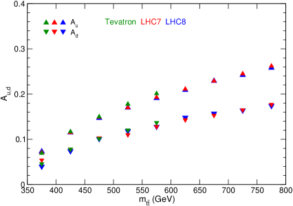
These tables show that the SM values of $A_{u,d}$ and $A^{\prime}_{u,d}$ computed for the Tevatron and the LHC, respectively, are in quite good agreement, which is remarkable given the difference of roughly one order of magnitude between the predictions for the inclusive asymmetries $A_{FB}$ and $A_{C}$. For illustration, in Fig. 1 the intrinsic asymmetries in Tables 1–3 are displayed, for $\mu=m_{t}$, as functions of $m_{t\bar{t}}$. For the Tevatron, only bins with $m_{t\bar{t}}<600$ GeV are included. These plots show the increase of these asymmetries with increasing $m_{t\bar{t}}$ and, furthermore, that the upper cut on $p_{T}^{t\bar{t}}$ reduces the slight difference between the Tevatron and LHC asymmetries, making them nearly equal. We remark that the differences exhibited in the left plot are irrelevant from an experimental point of view, as we shall see below. We also point out that the differences between the Tevatron and LHC results originate from Monte Carlo statistics to some extent, as it can be noticed from the fact that the smooth increase of the asymmetries with $m_{t\bar{t}}$ is modulated by small fluctuations.

Figure 1: Summary of asymmetries for the Tevatron and the LHC (7 and 8 TeV), for $\mu=m_{t}$, without $p_{T}^{t\bar{t}}$ cut (left) and for $p_{T}^{t\bar{t}}<30$ GeV (right). The data correspond to the first two columns of Tables 1–3.

As we have emphasized before, at the LHC the contributions from $gq$ processes to $A^{\prime}_{u,d}$ are quite small. This can be shown, for example, by using in the second of Eqs. (31) the SM values of $A_{C}^{q\bar{q}+gq}(\beta_{i})$ instead of $A_{C}^{q\bar{q}}(\beta_{i})$. The resulting intrinsic asymmetries are presented in Table 4 for 7 TeV, without $p_{T}^{t\bar{t}}$ cut. Comparison with the corresponding numbers of Table 2 shows that the differences are negligible. The differences are even further reduced if an upper cut on $p_{T}^{t\bar{t}}$ is applied.

Table 4: Asymmetries $A^{\prime}_{u,d}$ at the LHC (7 TeV), without $p_{T}^{t\bar{t}}$ cut, including $gq$ contributions.

	$\mu=m_{t}$		$\mu=2m_{t}$		$\mu=m_{t}/2$
$m_{t\bar{t}}$ [GeV]	$A^{\prime}_{u}$	$A^{\prime}_{d}$	$A^{\prime}_{u}$	$A^{\prime}_{d}$	$A^{\prime}_{u}$	$A^{\prime}_{d}$
$<400$	0.056	0.038	0.053	0.035	0.060	0.042
$400-450$	0.091	0.060	0.086	0.055	0.097	0.067
$450-500$	0.115	0.078	0.108	0.071	0.123	0.087
$500-550$	0.132	0.085	0.124	0.078	0.141	0.095
$550-600$	0.147	0.097	0.139	0.088	0.157	0.106
$600-650$	0.161	0.108	0.152	0.097	0.172	0.118
$650-700$	0.172	0.115	0.163	0.107	0.186	0.129
$700-750$	0.184	0.125	0.172	0.110	0.195	0.136
$750-800$	0.191	0.125	0.178	0.113	0.205	0.139

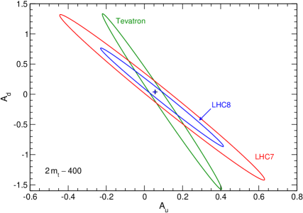
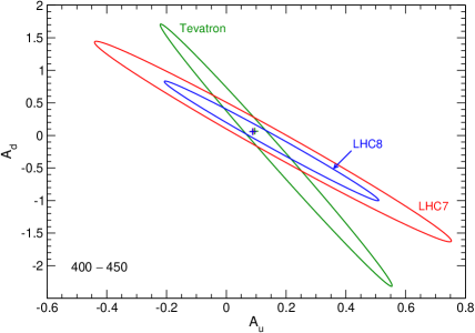
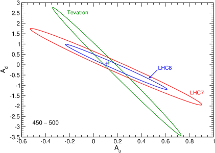
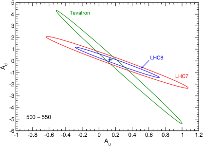
Next, we check the equivalence of the two- and one-dimensional fits in determining the intrinsic asymmetries. In Fig. 2 these asymmetries are plotted for the first four $m_{t\bar{t}}$ bins. The dots represent the values calculated with one-parameter fits (these are the numbers given in Tables 1-3), and the ellipses are the two-dimensional 68% confidence level (CL) regions from the 2-dimensional fit, where the centre is the best-fit value giving the minimum $\chi^{2}_{\text{min}}$ and the border corresponds to $\chi^{2}=\chi^{2}_{\text{min}}+2.3$, including statistical uncertainties only and assuming a perfect reconstruction of the $t$ and $\bar{t}$ momenta. From these plots, it is also clear that the slight differences between the Tevatron and LHC asymmetries are irrelevant as to the anticipated experimental uncertainty. This justifies the ansatz of extracting the same quantities from two different sets of data.

Figure 2: Comparison between asymmetries obtained with two- and one-dimensional fits, for $\mu=m_{t}$, without $p_{T}^{t\bar{t}}$ cut. The mass range in the lower left corner indicates the $m_{t\bar{t}}$ bin (in GeV). The ellipses represent the 68% CL regions for the two-dimensional fit, where only statistical uncertainties are considered.

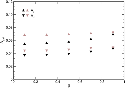
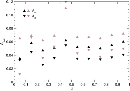
So far we have determined the intrinsic asymmetries $A^{\mbox{\tiny(${}^{\prime}$)}}_{u,d}$ by simulating the proposed fitting procedure with SM data: we have computed, for various $m_{t\bar{t}}$ bins, the binned asymmetries $A_{FB}(\beta_{i})$, $A_{C}(\beta_{i})$, the fractions $F^{\mbox{\tiny(${}^{\prime}$)}}_{q}$ and the dilution factors $D_{q}$ in the SM and performed the fits using Eqs. (31) and (LABEL:twofit). This leads, by definition, to constant $A^{\mbox{\tiny(${}^{\prime}$)}}_{u,d}$ for each $m_{t\bar{t}}$ bin. It remains to show that this is an acceptable procedure – i.e., that the $\beta$-binned intrinsic asymmetries are only mildly $\beta$-dependent within the $m_{t\bar{t}}$ bins chosen above, as it was claimed. This is shown in Fig. 3 for the first $m_{t\bar{t}}$ bin. (For the other $m_{t\bar{t}}$ bins the behavior is quite similar.) This variation can be compared, for example, with an increase in $F^{\prime}_{u}$ by a factor of 3 and $D_{u}$ ($D_{d}$) by factors of 20 (40), between the bins $0<\beta<0.1$ and $0.9<\beta<1$. These results corroborate the assumption of constant $A^{\mbox{\tiny(${}^{\prime}$)}}_{u,d}$, especially when an upper cut on $p_{T}^{t\bar{t}}$ is used. The LHC results shown in the plot in the right panel of Fig.3 exhibit some statistical fluctuations, which have some effect on the resulting fit values of of $A^{\prime}_{u,d}$.

Figure 3: Dependence of $A_{u,d}$ on $\beta$ in the SM, for $m_{t\bar{t}}<400$ GeV at the Tevatron (left) and the LHC with 7 TeV (right). Black and gray triangles correspond to no $p_{T}^{t\bar{t}}$ cut and cut $p_{T}^{t\bar{t}}<30$ GeV, respectively.

Finally we comment on the importance of the SM electroweak contributions Hollik:2011ps ; Kuhn:2011ri ; Bernreuther:2012sx of order $\alpha_{s}^{2}\alpha$ to the charge asymmetries $A_{u,d}$ and $A^{\prime}_{u,d}$. The dominant contributions are due to the photonic corrections Hollik:2011ps whose size with respect to the pure QCD asymmetries is roughly given by the ratio $R_{q}=(36Q_{q}Q_{t}/5)(\alpha/\alpha_{s})$. That is, these QED contributions amount to a positive correction of $\sim 25\%$ for $A^{\mbox{\tiny(${}^{\prime}$)}}_{u}$, while they are negative, $\sim-13\%$ for $A^{\mbox{\tiny(${}^{\prime}$)}}_{d}$. The pure QCD contributions to $A^{\mbox{\tiny(${}^{\prime}$)}}_{u,d}$ may of course be computed also with one of the generally available NLO QCD Monte Carlo programs, e.g. with the codes of Campbell:2012uf ; Frixione:2008ym . One should keep in mind, however, that in Monte Carlo computations one normalizes the asymmetries with NLO QCD denominators, while we have used denominators computed at LO QCD.

IV Conclusions

The formulae (3) allow to extract the intrinsic forward-backward asymmetries $A_{u,d}$ and $A^{\prime}_{u,d}$ from the Tevatron $t\bar{t}$ forward-backward asymmetry $A_{FB}$ and the LHC charge asymmetry $A_{C}$, respectively, if measured in suitably chosen bins of the $t\bar{t}$ invariant mass $m_{t\bar{t}}$ and longitudinal velocity $\beta$ of the $t\bar{t}$ system. We have shown under which conditions Eqs. (3) hold in the SM to NLO in the gauge couplings. Our derivations apply of course also to possible new physics contributions to these asymmetries. In particular, we have shown within the SM that the intrinsic asymmetries are indeed collider-independent and, furthermore, only mildly $\beta$-dependent for suitably narrow $m_{t\bar{t}}$ bins, especially if an upper cut on the $p_{T}^{t\bar{t}}$ of the $t\bar{t}$ samples is applied. This corroborates the proposal of AguilarSaavedra:2012va to use (3) with constant $A_{u}$ and $A_{d}$ for performing a two-parameter fit to the respective Tevatron and LHC data.

In order to apply Eqs. (3) to data analysis, one has to compute the fractions $F_{q}$ and factors $D_{q}$ in the SM, either to LO or NLO QCD for a specific PDF set and for chosen values of the renormalization and factorization scales. The outcome of the fits depend, of course, on these choices. Needless to say, this would be extremely valuable information. It has previously been shown, on a model-independent basis AguilarSaavedra:2012va as well as for specific new physics models Drobnak:2012cz ; Alvarez:2012ca ; Drobnak:2012rb , that current measurements of $A_{FB}$ at the Tevatron and $A_{C}$ at the LHC are compatible. Therefore, the comparison of the measured values $A_{u,d}^{\text{\tiny exp}}$ with their SM predictions $A_{u,d}^{\text{\tiny SM}}$ would reveal whether or not there is agreement with the SM – and if a deviation would be found, it would show whether it is located in $A_{u}$ or $A_{d}$, or in both. This could be achieved by a combination of the results from measurements at the Tevatron and the LHC (and by eventually testing whether they are consistent), and would be a big step forward in pinning down the origin of the new physics contribution(s), if there are any. The experimental determination of $A_{u}$ and $A_{d}$ will certainly be a challenge, as it will involve in general a 3-dimensional unfolding of the data with respect to $m_{t\bar{t}}$, $\beta$, and the (anti)top rapidity, but it is certainly worth the effort, for the aim of resolving this puzzle.

Acknowledgements

The work of J.A.A.S. has been supported by MICINN by projects FPA2006-05294 and FPA2010-17915, Junta de Andalucía (FQM 101, FQM 03048 and FQM 6552) and Fundação para a Ciência e Tecnologia (FCT) project CERN/FP/123619/2011. The work of W.B. was supported by DFG, SFB TR9 and that of Z.G. Si by NSFC and by Natural Science Foundation of Shandong Province.

References

- (1) J. A. Aguilar-Saavedra and A. Juste, arXiv:1205.1898 [hep-ph].
- (2) T. Aaltonen et al. [CDF Collaboration], Phys. Rev. D 83, 112003 (2011).
- (3) T. Aaltonen et al. [CDF Collaboration], CDF note 10807 (2012).
- (4) V. M. Abazov et al. [D0 Collaboration], Phys. Rev. D 84, 112005 (2011).
- (5) J. H. Kühn and G. Rodrigo, Phys. Rev. D 59, 054017 (1999).
- (6) O. Antunano, J. H. Kühn and G. V. Rodrigo, Phys. Rev. D 77, 014003 (2008).
- (7) L. G. Almeida, G. Sterman and W. Vogelsang, Phys. Rev. D 78, 014008 (2008).
- (8) W. Bernreuther and Z. -G. Si, Nucl. Phys. B 837, 90 (2010).
- (9) N. Kidonakis, Phys. Rev. D 84, 011504 (2011).
- (10) V. Ahrens, A. Ferroglia, M. Neubert, B. D. Pecjak and L. L. Yang, Phys. Rev. D 84, 074004 (2011).
- (11) W. Hollik and D. Pagani, Phys. Rev. D 84, 093003 (2011).
- (12) J. H. Kühn and G. Rodrigo, JHEP 1201, 063 (2012).
- (13) J. M. Campbell and R. K. Ellis, arXiv:1204.1513 [hep-ph].
- (14) W. Bernreuther and Z. -G. Si, Phys. Rev. D 86, 034026 (2012).
- (15) A. Djouadi, G. Moreau, F. Richard and R. K. Singh, Phys. Rev. D 82, 071702 (2010); P. H. Frampton, J. Shu and K. Wang, Phys. Lett. B 683, 294 (2010); Q. -H. Cao, D. McKeen, J. L. Rosner, G. Shaughnessy and C. E. M. Wagner, Phys. Rev. D 81, 114004 (2010); Y. Bai, J. L. Hewett, J. Kaplan and T. G. Rizzo, JHEP 1103, 003 (2011). M. Cvetic, J. Halverson and P. Langacker, arXiv:1209.2741 [hep-ph].
- (16) S. Jung, H. Murayama, A. Pierce and J. D. Wells, Phys. Rev. D 81, 015004 (2010); S. Jung, A. Pierce and J. D. Wells, Phys. Rev. D 83, 114039 (2011).
- (17) K. Cheung, W. -Y. Keung and T. -C. Yuan, Phys. Lett. B 682 (2009) 287; K. Cheung and T. -C. Yuan, Phys. Rev. D 83, 074006 (2011); J. Shelton and K. M. Zurek, Phys. Rev. D 83, 091701 (2011).
- (18) A. E. Nelson, T. Okui and T. S. Roy, Phys. Rev. D 84, 094007 (2011); J. A. Aguilar-Saavedra and M. Pérez-Victoria, JHEP 1109, 097 (2011); K. Blum, Y. Hochberg and Y. Nir, JHEP 1110, 124 (2011); P. Ko, Y. Omura and C. Yu, JHEP 1201, 147 (2012)
- (19) J. Shu, T. M. P. Tait and K. Wang, Phys. Rev. D 81, 034012 (2010); A. Arhrib, R. Benbrik and C. -H. Chen, Phys. Rev. D 82, 034034 (2010); I. Dorsner, S. Fajfer, J. F. Kamenik and N. Kosnik, Phys. Rev. D 81, 055009 (2010); I. Dorsner, S. Fajfer, J. F. Kamenik and N. Kosnik, Phys. Rev. D 82, 094015 (2010); Z. Ligeti, G. M. Tavares and M. Schmaltz, JHEP 1106, 109 (2011); B. Grinstein, A. L. Kagan, M. Trott and J. Zupan, Phys. Rev. Lett. 107, 012002 (2011).
- (20) R. Barcelo, A. Carmona, M. Masip and J. Santiago, Phys. Lett. B 707, 88 (2012); G. M. Tavares and M. Schmaltz, Phys. Rev. D 84, 054008 (2011); E. Alvarez, L. Da Rold, J. I. S. Vietto and A. Szynkman, JHEP 1109, 007 (2011); J. A. Aguilar-Saavedra and M. Pérez-Victoria, Phys. Lett. B 705, 228 (2011).
- (21) J. Cao, L. Wang, L. Wu and J. M. Yang, Phys. Rev. D 84, 074001 (2011); E. L. Berger, Q. -H. Cao, C. -R. Chen, C. S. Li and H. Zhang, Phys. Rev. Lett. 106, 201801 (2011); B. Bhattacherjee, S. S. Biswal and D. Ghosh, Phys. Rev. D 83, 091501 (2011); J. A. Aguilar-Saavedra and M. Perez-Victoria, Phys. Lett. B 701, 93 (2011); J. A. Aguilar-Saavedra and J. Santiago, Phys. Rev. D 85, 034021 (2012).
- (22) M. I. Gresham, I. -W. Kim and K. M. Zurek, Phys. Rev. D 83, 114027 (2011); J. L. Hewett, J. Shelton, M. Spannowsky, T. M. P. Tait and M. Takeuchi, Phys. Rev. D 84, 054005 (2011); G. F. Giudice, B. Gripaios and R. Sundrum, JHEP 1108, 055 (2011); U. Haisch and S. Westhoff, JHEP 1108, 088 (2011); S. Jung, A. Pierce and J. D. Wells, Phys. Rev. D 84, 091502 (2011); E. L. Berger, Q. -H. Cao, J. -H. Yu and C. -P. Yuan, Phys. Rev. D 84, 095026 (2011).
- (23) R. Diener, S. Godfrey and T. A. W. Martin, Phys. Rev. D 80, 075014 (2009).
- (24) G. Aad et al. [ATLAS Collaboration], Eur. Phys. J. C 72, 2039 (2012).
- (25) S. Chatrchyan et al. [CMS Collaboration], Phys. Lett. B 709, 28 (2012).
- (26) S. Chatrchyan et al. [CMS Collaboration], Phys. Lett. B 717, 129 (2012).
- (27) J. Drobnak, J. F. Kamenik and J. Zupan, Phys. Rev. D 86, 054022 (2012).
- (28) E. Alvarez and E. C. Leskow, arXiv:1209.4354 [hep-ph].
- (29) J. Drobnak, A. L. Kagan, J. F. Kamenik, G. Perez and J. Zupan, arXiv:1209.4872 [hep-ph].
- (30) J. A. Aguilar-Saavedra and M. Perez-Victoria, Phys. Rev. D 84, 115013 (2011).
- (31) S. Frixione and B. R. Webber, arXiv:0812.0770 [hep-ph].
- (32) P. M. Nadolsky, H. -L. Lai, Q. -H. Cao, J. Huston, J. Pumplin, D. Stump, W. -K. Tung and C. -P. Yuan, Phys. Rev. D 78, 013004 (2008).