Measuring the History of Cosmic Reionization using the 21-cm Difference PDF

Abstract

During cosmic reionization, the 21-cm brightness fluctuations were highly non-Gaussian, and complementary statistics can be extracted from the distribution of pixel brightness temperatures that are not derivable from the 21-cm power spectrum. One such statistic is the 21-cm difference PDF, the probability distribution function of the difference in the 21-cm brightness temperatures between two points, as a function of the distance between the points. Guided by 21-cm difference PDFs extracted from simulations, we perform a maximum likelihood analysis on mock observational data, and analyze the ability of present and future low-frequency radio array experiments to estimate the shape of the 21-cm difference PDF, and measure the history of cosmic reionization. We find that one-year data with an experiment such as the Murchison Wide-field Array should suffice for probing large scales during the mid-to-late stages of reionization, while a second-generation experiment should yield detailed measurements over a wide range of scales during most of the reionization era.

1 Introduction

In the coming decade, low-frequency radio arrays will begin to probe the epoch of reionization via the redshifted 21-cm hydrogen line. Current observational efforts include the MWA (Murchison Wide-field Array) (Bowman, Morales & Hewitt, 2009), LOFAR (Low Frequency Array) (Harker et al., 2010), PAPER (Precision Array for Probing the Epoch of Reionization) (Jacobs et al., 2011), and the GMRT (Giant Metrewave Radio Telescope) (Paciga et al., 2011). Successful interpretation of these observations will require effective statistical techniques for analyzing the data. Due to the difficulty of these measurements, it is important to develop techniques beyond the standard power spectrum analysis, in order to offer independent confirmation of the reionization history, probe different aspects of the topology of reionization, and do this with methods subject to different systematic errors.

During reionization, the hydrogen distribution is a highly non-linear function of the distribution of the underlying ionizing sources. A natural statistic for probing the expected non-Gaussianity is the one-point probability distribution function (PDF) of the 21-cm brightness temperature at a point (Furlanetto, Zaldarriaga & Hernquist, 2004; Ciardi & Madau, 2003; Mellema et al., 2006; Wyithe & Morales, 2007; Harker et al., 2009; Ichikawa et al., 2010; Gluscevic & Barkana, 2010). In this paper, we focus on the PDF $p_{\Delta}(\Delta T_{b})$ of the difference in 21-cm brightness temperature between two points in the cosmological volume, $\Delta T_{b}=|T_{2}-T_{1}|$. This 21-cm difference PDF, suggested by Barkana & Loeb (2008), is a two-dimensional function, dependent not only on $\Delta T_{b}$ but also on the separation $r$ between the two points at which the difference in brightness temperature is measured.

There are at least three advantages to the 21-cm difference PDF statistics (Gluscevic & Barkana, 2010), which we summarize here. Firstly, if the number of resolved cubic pixels (i.e., voxels) in the observed volume is $N$, the number of data points available for reconstructing the one-point PDF is only $N$, whereas the number of data points available for reconstructing the difference PDF ($N^{2}/2$) is overwhelmingly larger, albeit the latter data points must be sorted into bins of distance $r$. Thus, we might expect to do better than with the one-point PDF, which requires rather strong assumptions in order to allow a reconstruction of the reionization history with upcoming experiments (Ichikawa et al., 2010). Secondly, the 21-cm difference PDF generalizes both the one-point PDF and the two-point correlation function of $T_{b}$ (the latter of which can be deduced using the variance of the difference PDF, and is equivalent to the power spectrum), and also yields additional information beyond those statistics. Thirdly, the difference PDF avoids (by its very definition) the unwanted contribution of the mean sky background temperature, and is readily applicable to temperature differences measured with radio interferometry.

2 Methodology

We adopt the expected parameters for 1-year observations of a single field of view with MWA, using equations for 21-cm interferometer arrays from the review by Furlanetto, Oh & Briggs (2006), with an integration time of $t_{int}=1000$ hours, a collecting area of $A_{tot}\sim 2\times 10^{3}$ m², a field of view of $\pi 16^{2}$ deg² and a total bandwidth of $\Delta\nu_{\rm tot}=6$ Mhz. Note that the collecting area here is 4 times smaller than the collecting area assumed in Ichikawa et al. (2010), given the scaling down of the first generation of the MWA compared to earlier plans. Then, assuming cubic pixels of size $r_{\rm com}$ (all distances comoving), we find the following expected number of voxels $N_{p}$ and root-mean-square noise in each one $\sigma_{N}$:

$$N_{p} = 8.2\times 10^{7}\left(\frac{r_{\rm com}}{2.9\,\mbox{Mpc}}\right)^{-3}\left(\frac{1+z}{9}\right)^{0.9}\ ,$$ (1)

$$\sigma_{N} = 4400\left(\frac{r_{\rm com}}{2.9\,\mbox{Mpc}}\right)^{-2.5}\left(\frac{1+z}{9}\right)^{5.25}\mbox{mK}\ .$$ (2)

In order to look a bit ahead, we also consider specifications with lower noise in the same field of view, e.g., 1/2 the noise we denote as MWA/2 (which corresponds to 4-year data with the MWA), while 1/10 the noise we denote as MWA/10; the latter is a conservative estimate (by at least a factor of a few) for larger, second generation 21-cm arrays such as the SKA (Square Kilometer Array) or a 5000-antenna MWA. The only source of noise we consider is Gaussian thermal noise, whose magnitude is determined by the receiver’s system temperature, which is set by the sky’s brightness temperature dominated by Galactic synchrotron emission (Furlanetto, Oh & Briggs, 2006). This assumes perfect foreground removal from 21-cm maps. Clearly, the first step for any proposed measurement method is to prove its feasibility against thermal noise, which can then motivate more detailed analyses that include a larger range of observational difficulties and sources of noise.

2.1 Model PDF and Thermal Noise

We begin by considering a general PDF, which could be the regular (one-point) PDF or the difference PDF. To determine a best-fit PDF using observed data, we characterize the PDF with a finite number of parameters. We do so with a binned PDF, expressed as the sum of boxcar functions for each bin $p(x)=\sum F_{i}(x)$, where

$$F_{i}(x)=\left\{\begin{array}[]{l l}l_{i}&\quad\textrm{if $a_{i}<x<a_{i+1}$}\\ 0&\quad\textrm{otherwise.}\\ \end{array}\right.$$ (3)

Here $l_{i}$ is the bin height, and the probability contained in bin $i$ is $p_{i}=l_{i}(a_{i+1}-a_{i})$. In a model with $N_{b}$ bins where the bin edges $\{a_{1},a_{2},\ldots,a_{N_{b}+1}\}$ are fixed, the binned PDF only has $N_{b}-1$ free parameters $\{l_{1},l_{2},\ldots,l_{N_{b}-1}\}$, as $l_{N_{b}}$ must be normalized such that the probabilities sum up to unity. Note that throughout this paper we use this very general binned form for the PDF, and do not need to assume a particular functional form for the difference PDF as is necessary for the one-point PDF given its much lower signal-to-noise ratio (Ichikawa et al., 2010).

Theoretically, the measured PDF will be the true PDF convolved with the noise. For example, the 21-cm brightness temperature one-point PDF measured by instruments will be the true one-point PDF $p(T)$ convolved with an extremely broad normal distribution:

$$N(0,\sigma_{N}^{2})=\frac{1}{\sqrt{2\pi}\,\sigma_{N}}\,e^{-\frac{T^{2}}{2\sigma^{2}_{N}}}\ ,$$ (4)

with zero mean and standard deviation $\sigma_{N}$ due to thermal noise (Equation (2)). Hence, the noisy one-point PDF can be expressed as a sum of the convolution of boxcar functions with the Gaussian,

$$p_{\rm noisy}(T)=\sum F_{i}(T)\star N(0,\sigma_{N}^{2})\ ,$$ (5)

where

$$F_{i}(T)\star N(0,\sigma_{N}^{2})=\frac{1}{2}l_{i}\left[\mbox{Erf}\left(\frac{T-a_{i}}{\sqrt{2}\,\sigma_{N}}\right)-\mbox{Erf}\left(\frac{T-a_{i+1}}{\sqrt{2}\,\sigma_{N}}\right)\right].$$ (6)

Here $\mbox{Erf}(x)$ is the error function. $p_{\rm noisy}(T)$ can be used to generate mock observations of the one-point PDF.

Out of symmetry and convenience, the difference PDF $p_{\Delta}(\Delta T_{b})$ defined in the literature (Barkana & Loeb, 2008) is a function of the absolute difference in brightness temperature $\Delta T_{b}=|T_{2}-T_{1}|$. However, to find the effect of thermal noise on the difference PDF $p_{\Delta,\rm noisy}(\Delta T_{b})$, it is easier to first find the probability distribution function $p_{\Delta,\rm noisy}(\Delta T_{21})$ as a function of the temperature difference $\Delta T_{21}\equiv T_{2}-T_{1}$ without the absolute value. If the thermal noise at any two points 1 and 2 is uncorrelated, then their temperature difference has a root-mean-square thermal noise of $\sqrt{2}\,\sigma_{N}$. If the intrinsic difference PDF is $p_{\Delta}(\Delta T_{21})$, the observed version is then:

$$p_{\Delta,\rm noisy}(\Delta T_{21})$$ (7)

$$= p_{\Delta}(\Delta T_{21})\star N(0,2\sigma_{N}^{2})$$

$$= \sum F_{i}(\Delta T_{21})\star N(0,2\sigma_{N}^{2})$$

$$= \sum\frac{1}{2}l_{i}\left[\mbox{Erf}\left(\frac{\Delta T_{21}-a_{i}}{2\sigma_{N}}\right)-\mbox{Erf}\left(\frac{\Delta T_{21}-a_{i+1}}{2\sigma_{N}}\right)\right].$$

Now, due to symmetry, $p_{\Delta,\rm noisy}(\Delta T_{21})$ is an even function, so we can recover the difference PDF as defined for the absolute temperature differences, with thermal noise included, via

$$p_{\Delta,\rm noisy}(\Delta T_{b})=\left\{\begin{array}[]{l l}2\>p_{\Delta,\rm noisy}(\Delta T_{21})&\quad\textrm{if $\Delta T_{21}\geq 0$}\\ 0&\quad\textrm{otherwise}\ .\\ \end{array}\right.$$ (8)

To use equation (7), we need to assume a true difference PDF, with which to convolve the thermal noise. To this end, we use the binned difference PDF as measured in the fiducial $S1$ simulation of McQuinn et al. (2007), who modeled the density field during the epoch of reionization with a $1024^{3}$ N-body simulation in a box size of $\approx 94$ Mpc, post-processing it using a suite of radiative-transfer simulations to characterize the morphology and size distribution of ionized regions during reionization. Analytic prescriptions were used to model reionization effects of small-scale structure that was unresolved in the N-body simulation. Source parameters were chosen so that reionization ends near $z=7$ in the simulation.

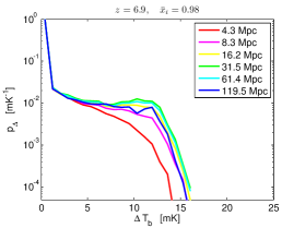
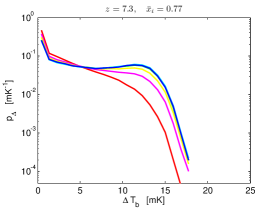
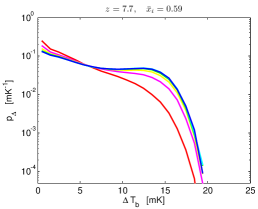
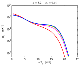
The 21-cm difference PDF’s from these simulations, shown in Figure 1, were first presented by Gluscevic & Barkana (2010); here we use the same redshift slices (taken at 50 Myr intervals), the same cubic voxel size of 2.9 (comoving) Mpc, and the same logarithmically spaced distance bins to obtain the ‘true’ difference PDF from the simulation. The central values of the logarithmic distance bins are $r_{\rm mid}=$ 4.3, 8.3, 16.2, 31.5, 61.4, and 119.5 Mpc. However, instead of using the same 20 linearly spaced temperature bins as Gluscevic & Barkana (2010), we alternate the number and interval size of our temperature bins $\{a_{1},a_{2},\ldots,a_{N_{b}+1}\}$, to see the dependence of the fit errors on the number of free parameters. In general, reducing the number of bins gives a more accurate determination of the PDF, but at the price of less detailed information on its shape, since the measured PDF is (at best) the true one but smoothed on the scale of the bin size.

(a)

(b)

(c)

(d)

(e)

(f)

(g)

(h)

(i)

Figure 1: 21-cm difference PDFs from Gluscevic & Barkana (2010) are shown here as a function of their distance bin and redshift. The legend in the first panel indicates the central values $r_{\rm mid}$ of the logarithmic distance bins.

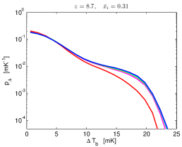
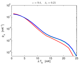
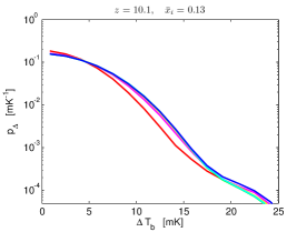
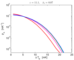
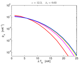
Mock observational difference PDF values can be created by randomly generating $n$ values of $\Delta T_{b}$ using the distribution $p_{\Delta,\rm noisy}(\Delta T_{b})$. The same functional form can be employed in finding the best fit parameters $\{l_{i}\}$ to the same mock observations with a maximum likelihood method. In this paper, we sample each difference PDF and generate 1000 Monte Carlo instances of observational data for that model, and thus obtain a well-sampled distribution of reconstructed model parameters.

2.2 Number of Voxel Pairs

For a given observational volume, voxel size, and distance $r$ between pairs of voxels, the number of voxel-pairs $N(r)dr$ (at distances between $r$ and $r+dr$) is uniquely determined. Thus, for each bin we sample $n=\int N(r)dr$ values of $\Delta T_{b}$ from $p_{\Delta,\rm noisy}(\Delta T_{b})$ as our mock data.

With the edge size of each voxel normalized to 1, the number of voxel-pairs in a cubic volume $V=L^{3}$ as a function of the voxel distance $r$ can be closely approximately by the number of voxel-pairs in a sphere of the same volume $V=4\pi R^{3}/3$ at the same distance, at least for small $r$. A sphere is easier to analyze, and yields an analytical result for the voxel-pair distribution function:

$$N(r)\,dr=\frac{1}{6}\pi^{2}r^{2}(2R-r)^{2}(4R+r)\,dr\ .$$ (9)

Equation (9) is exact for spherical volumes for all $r\in(0,2R)$, in the limit of infinitesimal $dr$ and voxel size (compared to $r$ and $R$). The total number of voxel pairs at all $r$ in a sphere of radius $R$ is

$$\int_{0}^{2R}N(r)\,dr=\frac{1}{2}\left(\frac{4}{3}\pi R^{3}\right)^{2},$$ (10)

which is $\frac{1}{2}N^{2}$ as expected, in terms of the total number of voxels $N$.

If the distance between voxel-pairs is much less than the characteristic size of the observable volume, then the total number of voxel-pairs at that small distance will not be sensitive to the shape of the volume, but only to its size. In considering such a pair, voxel #1 can be chosen anywhere within the volume, and #2 must then be at a distance $r$ in any direction. As long as $r\ll L$ (or $r\ll R$), the full sphere of radius $r$ about # 1 will almost always fall within the big volume, so that all #2 voxels on this small sphere are allowed. Thus, the number of pairs will be the number of #1 voxels $V$ times the number of #2 voxels $4\pi r^{2}\,dr$, divided by 2 for double-counting of pairs. The result of $2\pi Vr^{2}\,dr$ agrees with equation (9) in the small-$r$ limit. Corrections to this result will come from cases where pixel #1 is within a distance $r$ of the volume’s boundary, i.e., the correction is of order the surface area times $r$ divided by the volume, which (for simply-connected convex volumes such as a sphere or cube) is of order $r/V^{1/3}$.

For the MWA, if we assume that the volume it will observe on the sky is approximately cubic, equation (1) implies that the length of the cube $L\sim 1000$ Mpc for all redshifts of interest. This is much greater than the largest distance ($r\sim 163$ Mpc) between voxel-pairs we consider in this paper. Since $L\gg r$, we use equation (9) as an excellent proxy for the number of voxel-pairs MWA will observe, and list the values of $\int N(r)dr$ in each distance bin in Table 1.

Table 1: The number of voxel-pairs $\int N(r)dr$ in each distance bin, as a function of redshift. The distance bins are logarithmically spaced and are denoted via their central values $r_{\rm mid}$, in units of (comoving) Mpc. The size of each voxel is chosen to be 2.9 Mpc, consistent with Gluscevic & Barkana (2010), from which the simulated difference PDFs were taken. Due to equation 1, the total number of voxels (and thus $N(r)$) has a slight redshift dependence. Higher separation bins $r_{\rm mid}$ have orders of magnitude more voxel-pairs compared to lower $r_{\rm mid}$, varying roughly as $r^{3}$ when $r\ll L$ (since the bin width $\propto r$).

$r_{\rm mid}=$	4.3	8.3	16.2	31.5	61.4	119.5
$z=6.9$	1.1E9	8.3E9	6.1E10	4.4E11	3.1E12	2.2E13
$z=7.3$	1.2E9	8.7E9	6.4E10	4.6E11	3.3E12	2.3E13
$z=7.7$	1.2E9	9.1E9	6.6E10	4.8E11	3.4E12	2.4E13
$z=8.2$	1.3E9	9.6E9	7.0E10	5.1E11	3.6E12	2.5E13
$z=8.7$	1.4E9	1.0E10	7.3E10	5.3E11	3.8E12	2.6E13
$z=9.4$	1.5E9	1.1E10	7.8E10	5.7E11	4.1E12	2.8E13

2.3 Maximum Likelihood for a Multinomial Distribution

Since $n$ is large, to compare the mock observational data to a potential model, we also bin the observational data into $N_{B}$ bins (in general different from the number of bins $N_{b}$ in the model). Note that a binned PDF is essentially a multinomial distribution of the variable $X$ given by the set of bin probabilities $\mathbf{p}=(p_{1},\ldots,p_{N_{B}})$; given $n$ total data points, there will be an expected number of $n_{\mbox{exp},j}=n\>p_{j}$ data points in bin $j$. As for the covariance matrix $\Sigma$, the variance of $X$ in a single bin $j$ is $p_{j}(1-p_{j})$, while the covariance between different bins $i$, $j$ is $-p_{i}p_{j}$. How does one account for the covariance structure of a multinomial distribution in a maximum likelihood estimate (MLE) fit?

In the limit of large $n$, the multinomial distribution is approximated by the multivariate normal distribution with the same mean $\mathbf{p}$ and covariance $\Sigma$. We apply MLE to this multivariate normal with model parameters $\mathbf{p}^{\ast}=(p_{1},\ldots,p_{N_{B}-1})$, where we drop the last bin $p_{N_{B}}$ because it is not an independent variable due to normalization constraints, and none of the elements in $\Sigma$ are free variables as they are completely determined by $\mathbf{p}^{\ast}$. We thus find that the objective function to be minimized is:

$$(\Delta X^{\ast})^{T}(\Sigma^{\ast})^{-1}(\Delta X^{\ast}),$$ (11)

where $X^{\ast}$ refers to the first $N_{B}-1$ bins, so that the vector

$$\Delta X^{\ast} = \overline{X^{\ast}}-\mathbf{p}^{\ast}$$ (12)

$$= (\overline{X_{1}}-p_{1},\ldots,\overline{X_{N_{B-1}}}-p_{N_{B}-1})$$

is the deviation between the observed probabilities $\overline{X^{\ast}}$ and model probabilities $\mathbf{p}^{\ast}$. Note that by definition $\overline{X_{j}}=n_{j}/n$, where $n_{j}$ is the actual number of data points observed in bin $j$. Similarly, $\Sigma^{\ast}$ is the covariance matrix of $X^{\ast}$, and is equal to the upper-left $(N_{B}-1)\times(N_{B}-1)$ submatrix of $\Sigma$. Note that this approach correctly accounts for the constraint of the total probability summing up to unity.

$\Sigma^{\ast}$ is indeed invertible, and takes the form:

$$(\Sigma^{\ast})^{-1}=\left(\begin{array}[]{cccc}\frac{1}{p_{1}}+\frac{1}{p_{N_{B}}}&\frac{1}{p_{N_{B}}}&\ldots&\frac{1}{p_{N_{B}}}\\ \frac{1}{p_{N_{B}}}&\frac{1}{p_{2}}+\frac{1}{p_{N_{B}}}&\ldots&\frac{1}{p_{N_{B}}}\\ \vdots&\vdots&\ddots&\vdots\\ \frac{1}{p_{N_{B}}}&\frac{1}{p_{N_{B}}}&\ldots&\frac{1}{p_{N_{B}-1}}+\frac{1}{p_{N_{B}}}\end{array}\right)\ .$$ (13)

Thus, we find that the objective function

$$(\Delta X^{\ast})^{T}(\Sigma^{\ast})^{-1}(\Delta X^{\ast})$$ (14)

$$= \left(\frac{\overline{X_{1}}}{p_{1}}-\frac{X_{N_{B}}}{p_{N_{B}}},\ldots,\frac{\overline{X_{N_{B-1}}}}{p_{N_{B-1}}}-\frac{X_{N_{B}}}{p_{N_{B}}}\right)^{T}(\Delta X^{\ast})$$

$$= \sum_{j=1}^{N_{B}}\frac{(\overline{X_{j}}-p_{j})^{2}}{p_{j}}$$

$$= \frac{1}{n}\sum_{j=1}^{N_{B}}\frac{(n_{j}-n_{\mbox{exp},j})^{2}}{n_{\mbox{exp},j}}$$

$$= \frac{1}{n}\chi^{2},$$

where $\chi^{2}$ is the standard Pearson’s chi-squared statistic. In summary, to find the best MLE fit for a multinomial distribution of $N_{B}$ components with $N_{B}-1$ free parameters, one can simply minimize a standard $\chi^{2}$ statistic in which all $N_{B}$ terms in the $\chi^{2}$ are summed over.

We bin the values from the mock observation data into $N_{B}=1,000$ bins; this is justified as long as the bin width is much smaller than any scale we hope to resolve in the observed PDF. We leave the last bin at the tail of the observed difference PDF with a much wider width than the other bins, so that each bin has more than 10 counts (with most having a vastly larger count number), and we do not have to use the $C$-statistic (Cash, 1979) instead to account for large relative errors at small counts.

3 Results

3.1 1-bin model

The attempt to measure the difference PDF is essentially a contest between a very high level of noise per measurement (almost three orders of magnitude larger than the width of the intrinsic difference PDF in Figure 1) and a very large number of measurements. A naive signal-to-noise estimate may suggest that only $\sim 10^{6}$ measurements (i.e., the square of the noise-to-signal ratio of each measurement) are needed for a rough measurement of a given difference PDF value (in some bin of temperature difference). In reality, though, the needed number is significantly higher, because of the near-degeneracy that is encountered in what is essentially an attempt to deconvolve the noisy difference PDF (see Ichikawa et al. (2010) for a detailed discussion in the context of the one-point PDF). Thus, it is prudent to start out conservatively, and try to fit a small number of bins.

Luckily, theory suggests that even a 1-bin model is worth considering, since it can yield valuable information. Such a model consists of a single bin at $\Delta T_{b}\approx 0$, plus a normalization bin at higher values. of $\Delta T_{b}$. The value of the total probability $p_{1}$ of the difference PDF in this first bin can be used as an approximation of $\Delta P_{D}$, which refers to the theoretical limit of a component of $\Delta P$ which is a Dirac Delta function at $\Delta T_{b}=0$ (Gluscevic & Barkana, 2010). This $\Delta P_{D}$ effectively measures a low-resolution version of the ionization correlation function during cosmic reionization (Barkana & Loeb, 2008); in the limit of perfect resolution, $\Delta P_{D}$ would exactly correspond to the joint ionization probability of two points as a function of their distance $r$. In this limit, at $r\rightarrow 0$, $\Delta P_{D}$ should simply equal the probability of having $T_{b}=0$ mK, which is the mean ionized fraction $\overline{x}_{i}$, and $\Delta P_{D}$ should decrease with increasing $r$ as the pair-correlation drops, until $\Delta P_{D}\approx\overline{x}_{i}^{2}$ at $r\rightarrow\infty$ (for which each voxel in the pair is ionized independently). As long as the ionized regions maintain a low (even if non-zero) neutral fraction, this description should be approximately valid even for the realistic difference PDF.

We begin with a 1-bin model consisting of a first bin between $\Delta T=0$ to 4 mK, plus a normalization bin at $\Delta T=4$ to 40 mK. Figure 2 illustrates the main results for this one-parameter model with one-year MWA noise. Even with this relatively large noise, the high number of voxel pairs in the observational volume of MWA drives the finite sampling noise to quite low levels, in many cases allowing us to overcome the degeneracy in the reconstruction. The value of the difference PDF in the first bin can be measured with an accuracy of a few percent for the larger voxel-pair distances $r_{\rm mid}=$ 61.4 and 119.5 Mpc, with some useful measurements possible at lower radii. The measurements are particularly advantageous at low redshift, where the high ionization fraction produces a large $\Delta P_{D}$ feature in the intrinsic difference PDF (Figure 1); this makes the measurement easier, and also makes the measured value more closely related to the ionization fraction. Indeed, the strong rise with time in the measured 1-bin $p_{1}$, occurring simultaneously at all $r$ bins, constitutes a clear detection of the end of reionization (at $z=6.9$ in this case).

Figure 2: Measured value and error of the total probability $p_{1}$ in the first bin ($\Delta T=0-4$ mK) of a 1-bin model of the difference PDF. We show this as a function of redshift, assuming MWA noise, for various voxel-pair distance bins: $r_{\rm mid}=$ 4.3, 8.3, 16.2, 31.5, 61.4, and 119.5 comoving Mpc (panels from top to bottom). We compare in each case the true value (green square), the mean fit value (red dot), and 16-84 percentile values (red error bars) based on 1,000 instances of mock observation data; we refer to these percentile values as the $\pm 1\sigma$ range in the rest of this paper. We also show the $\pm 1\sigma$ errors magnified by a factor of 10 (blue error bars), so that smaller errors are easier to see.

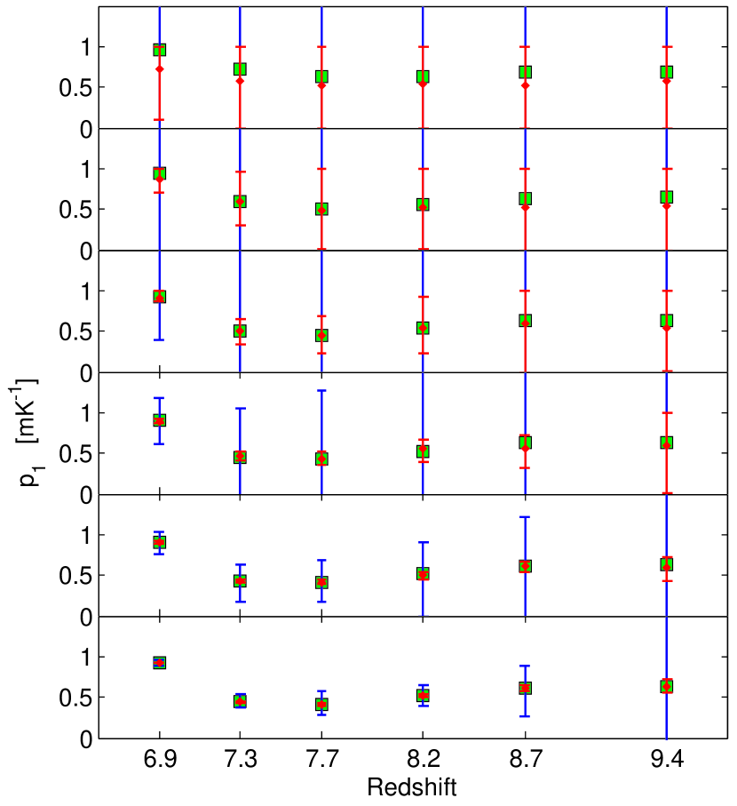
As shown in Figure 3, decreasing the noise by a factor of 2 (MWA/2) often decreases the errors in the reconstructed difference PDF by a factor of $3-4$, yielding some information even at the lowest values of $r$. Since values of $r\sim 10$ Mpc are required to see the variation of $p_{\Delta}$ with distance (Figure 1), this lower noise would allow us to get an indication of the average size of ionized bubbles, above which the correlation strength (and $p_{1}$) drops.

Figure 3: Same as Figure 2, but for MWA/2 noise, corresponding to 4 years of observations with the MWA.

Figures 4, 5 and 6 give a more complete indication of how the fit error varies with the thermal noise, at the end, middle, and beginning of the epoch of reionization, respectively. Again, we find that the larger distance bins have smaller errors because they have far more voxel-pairs, reducing the sampling error. Above some high level of noise, the degeneracy is complete and the fit error is of order unity regardless of the noise per pixel $\sigma_{N}$ (note that the probability within a bin is limited to vary between 0 and 1). However, below some critical value (which varies with $r$ due to the different numbers of voxel-pairs), the fit error begins to decrease as $\sigma_{N}$ decreases. This decrease is faster than linear (typically close to quadratic) since reduced noise removes some of the partial degeneracy involved in the effective deconvolution of $p_{\Delta}$. Note that the low noise levels we consider can correspond either to multi-year observations with the MWA or to future radio arrays with a larger collecting area.

Figure 4: Relative error of the measured $p_{1}$ in the first bin ($\Delta T=0-4$ mK) of the 1-bin model as a function of noise at $z=6.9$, when the mean ionization fraction was $\overline{x}_{i}=0.98$. Here the noise improvement factor is the factor by which the thermal noise is reduced compared to 1-year MWA observations (equation (2)). The relative error is defined as the range between the $\pm 1\sigma$ values divided by the true value.

Figure 5: Same as Figure 4 but at $z=8.2$, when $\overline{x}_{i}=0.44$.

Figure 6: Same as Figure 4 but at $z=10.1$, when $\overline{x}_{i}=0.13$.

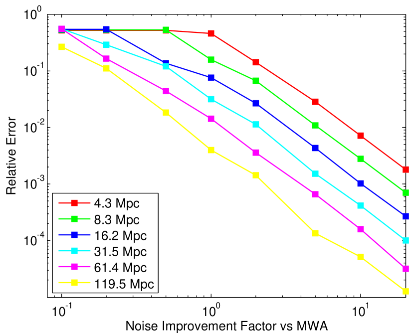
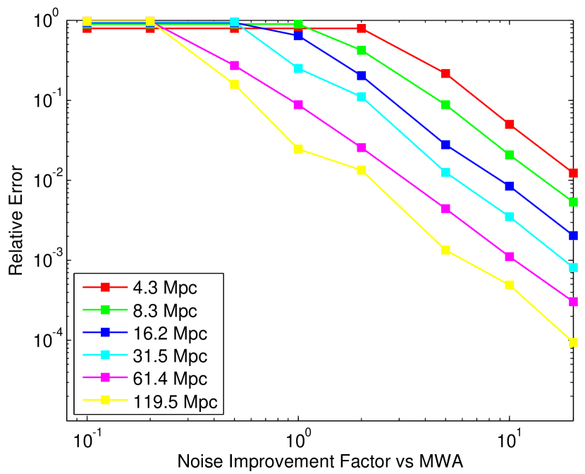
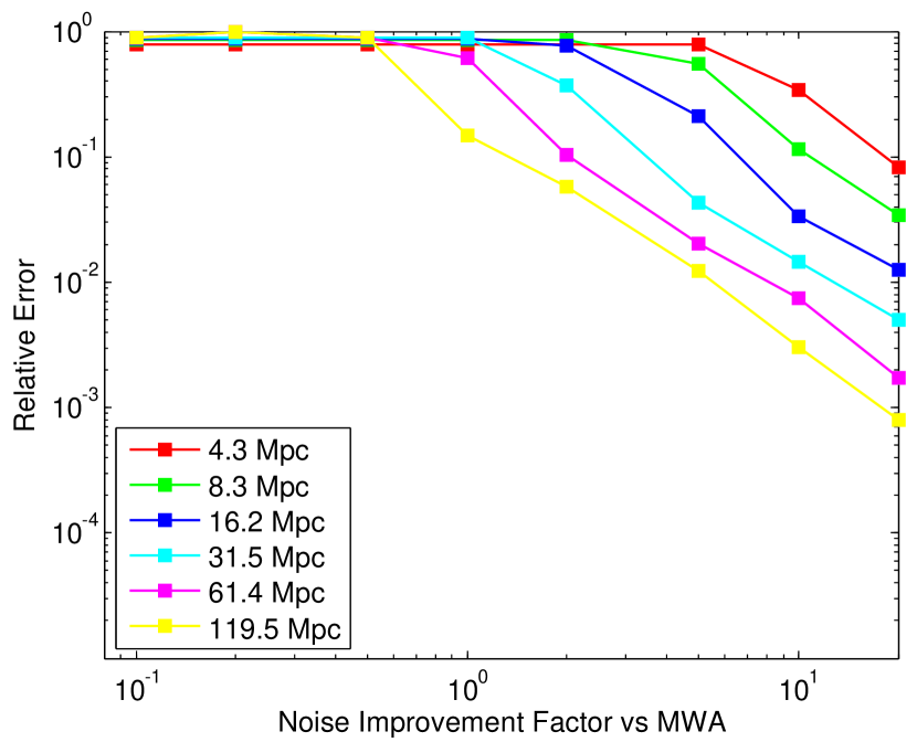
At $z=6.9$, the MWA suffices to measure the 1-bin difference PDF with $<10\%$ errors down to the $r=16$ Mpc bin, and thus verify the signature of the end of reionization. At the larger separations, the MWA can determine $p_{\Delta}$ to better than a percent. Higher redshifts are more challenging, so that at $z=8.2$ (near the midpoint of reionization), $<10\%$ errors are possible with the MWA only at the two highest separations, MWA/2 gets down to $\sim 30$ Mpc, and MWA/10 allows measurements at the full range of separations. Early in reionization ($z=10.1$), when the measurement noise is larger due to the higher redshift, and the difference PDF is still close to the Gaussian shape driven by density fluctuations, the MWA can only attempt to measure the long-separation limit of $p_{\Delta}$, but a second-generation experiment should still be able to probe a broad range of distances.

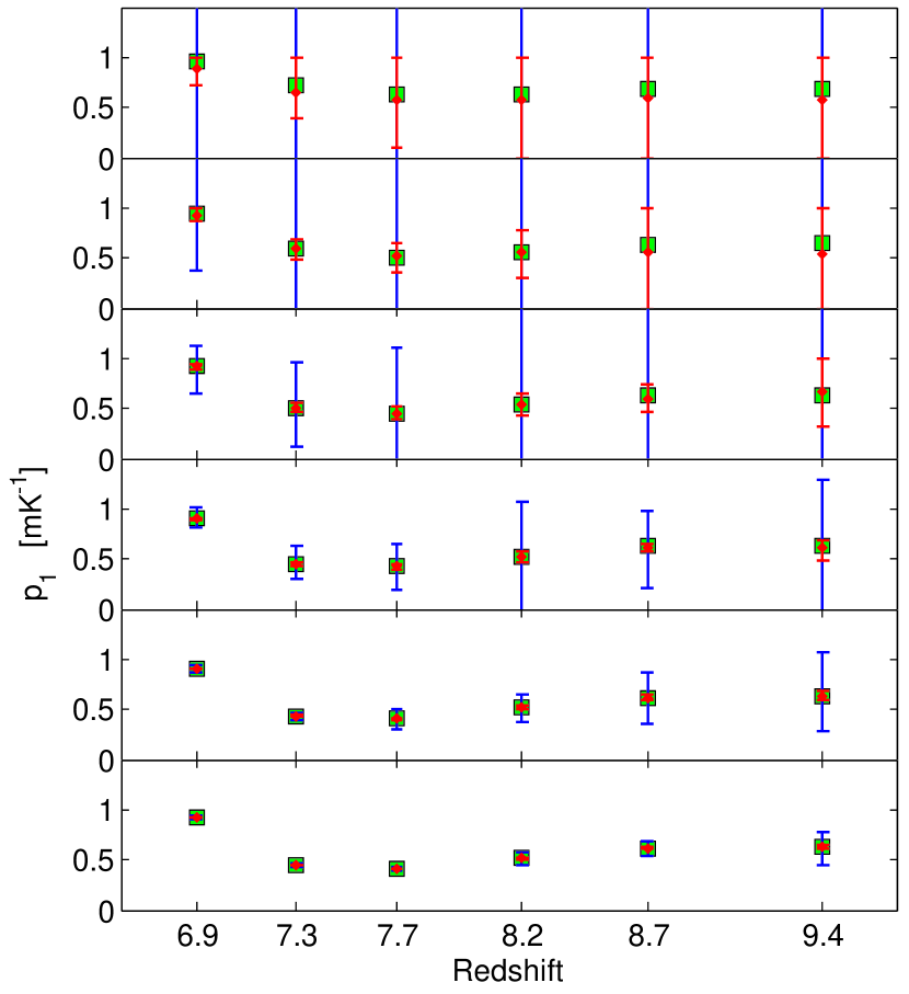
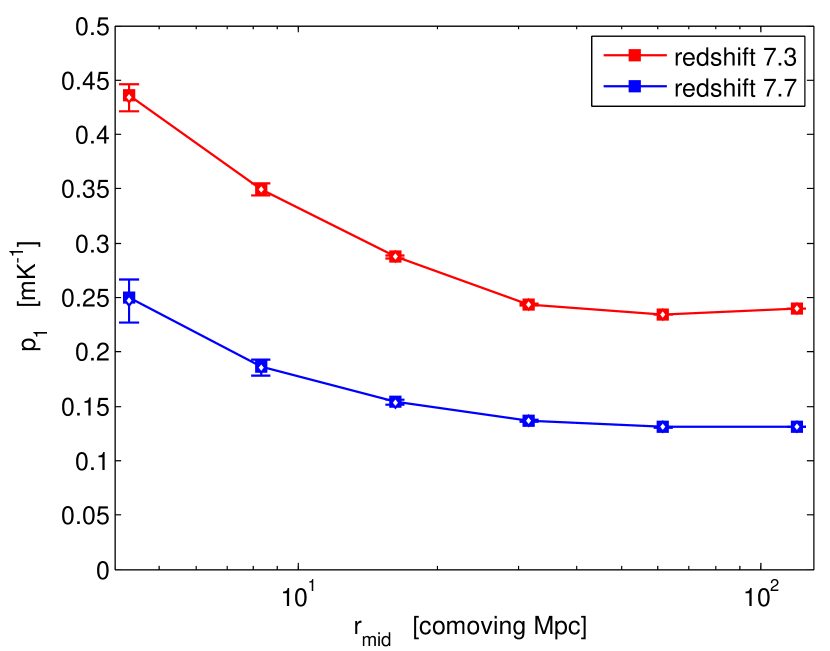
Alternatively, we can use a 1-bin model where the first bin is smaller, between $\Delta T=0$ to 1 mK. This pinpoints the fraction of voxel-pairs with $\Delta T_{b}\approx 0$ (which approximates $\Delta P_{D}$) more accurately. Thus, $p_{1}$ is significantly lower than with the wider first bin consider before, except at the very end of reionization. The measurement errors are generally similar to before, as illustrated for MWA/2 noise in Figure 7, which can be compared to Figure 3 from before. Figure 8 uses a different presentation to show more directly how with second-generation radio arrays we can accurately map $\Delta P_{D}$ as a function of $r$ across different redshifts, with the location of the flat asymptote of $p_{1}$ telling us where $r$ drops below the correlation length, which can be used to determine the average size of ionized bubbles. We note that one conservative way to begin investigating the shape of the difference PDF is to fit 1-bin models with various bin widths and compare the results. However, a more direct method is to use models with more bins, which we consider next.

Figure 7: Measured value and error of the total probability $p_{1}$ in the first bin of a 1-bin model of the difference PDF. Same setup and notation as in Figure 2, but with MWA/2 noise as in Figure 3, and here using a model with a narrower first bin ($\Delta T=0-1$ mK).

Figure 8: Measured value and error of the total probability $p_{1}$ in the first bin ($\Delta T=0\sim 1$ mK) of a narrow 1-bin model of $p_{\Delta}$, shown as a function of voxel-pair distance (bin center), with MWA/10 noise.

3.2 10-bin model

Given that the 1-bin model is expected to yield accurate measurements of the difference PDF, even better than $1\%$ measurements in some cases, we now consider a more ambitious attempt to measure the detailed shape of the difference PDF. We consider a 10-bin model consisting of 10 equal-size bins between $\Delta T=0$ and $10$ mK, plus a normalization bin at $\Delta T=10$ to 40 mK. Of course, many other binning choices are possible, including redshift-dependent binning, but our choice should suffice to determine whether the shape of the PDF can be determined with 1 mK bins over a range where there is interesting dependence on $\Delta T$ throughout the reionization era.

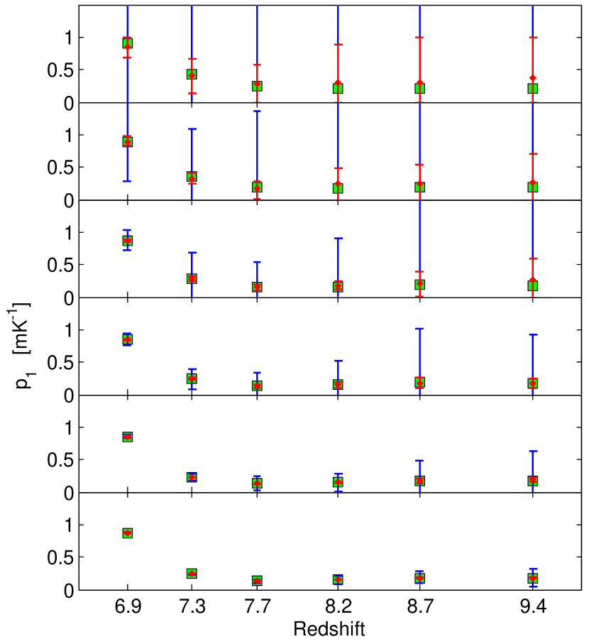
Near the end of reionization, we illustrate the expected reconstruction accuracy in three separation bins, $r_{\rm mid}=$ 16.2 (Figure 9), 61.4 (Figure 10) and 119.5 Mpc (Figure 11). While the theoretical difference PDF should have a simple shape, with nearly all the probability concentrated in the first bin, it would be exciting to directly verify this observationally. At 16.2 Mpc, the error in the first bin is very large, and there are strong degeneracies among the various bins, as illustrated by the failure of the fitting errors to decrease in going from MWA to MWA/2 errors. The degeneracy is broken, however, with MWA/10 errors, in which case the expected shape of $p_{\Delta}$ can be precisely verified. We note that the $r_{\rm mid}=$ 8.3 Mpc bin (not shown) shows similar reconstruction errors to the 16.2 Mpc case (except that the errors are larger by a factor of a few for MWA/10). At the two largest-separation bins, $p_{\Delta}$ can be reasonably measured with MWA/2 (for $r_{\rm mid}=$ 61.4 Mpc) or even with MWA errors (for the highest $r$ bin).

(a) Subfigure 1 list of figures text

(b) Subfigure 1 list of figures text

(c) Subfigure 2 list of figures text

Figure 9: Measured value and $1-\sigma$ error of $p_{\Delta}$ in the 10-bin model, at $z=6.9$, in the $r_{\rm mid}=16.2$ Mpc bin, shown for three different levels of the thermal noise (as indicated in each panel). We compare the true, input difference PDF (black line) in 10 bins of width 1 mK (an extra normalization bin for at $\Delta T>10$ mK is not shown) to the mean value and $16-84$ percentile range of the reconstructed $p_{\Delta}$ based on fitting to 1,000 mock data sets.

(a) Subfigure 1 list of figures text

(b) Subfigure 1 list of figures text

(c) Subfigure 2 list of figures text

Figure 10: Same as Figure 9 but for the $r_{\rm mid}=61.4$ Mpc bin.

(a) Subfigure 1 list of figures text

(b) Subfigure 1 list of figures text

(c) Subfigure 2 list of figures text

Figure 11: Same as Figure 9 but for the $r_{\rm mid}=119.5$ Mpc bin.

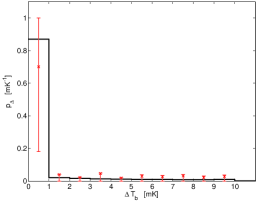
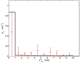
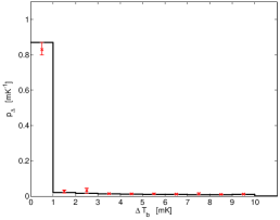
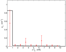
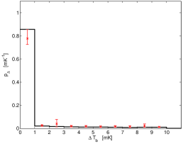
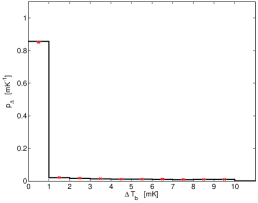
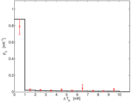
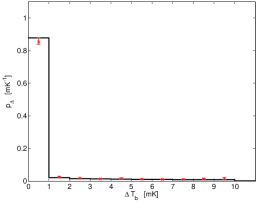
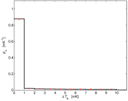
Near the midpoint of reionization, we illustrate the results for the same three separation bins, in Figures 12, 13, and 14. The results here are similar, in that useful measurements require MWA/10 errors for $r_{\rm mid}=16.2$ Mpc, MWA/2 for $r_{\rm mid}=61.4$ Mpc, and just MWA at the highest separation. Here again the $r_{\rm mid}=$ 8.3 Mpc bin (not shown) is similar to the 16.2 Mpc case, except for significantly less accurate (though still useful) measurements for MWA/10.

(a) Subfigure 1 list of figures text

(b) Subfigure 1 list of figures text

(c) Subfigure 2 list of figures text

Figure 12: Same as Figure 9 (i.e., $r_{\rm mid}=16.2$ Mpc) but at $z=8.2$.

(a) Subfigure 1 list of figures text

(b) Subfigure 1 list of figures text

(c) Subfigure 2 list of figures text

Figure 13: Same as Figure 12 but for the $r_{\rm mid}=61.4$ Mpc bin.

(a) Subfigure 1 list of figures text

(b) Subfigure 1 list of figures text

(c) Subfigure 2 list of figures text

Figure 14: Same as Figure 12 but for the $r_{\rm mid}=119.5$ Mpc bin.

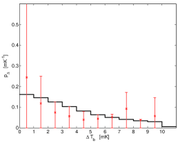
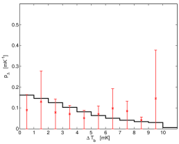
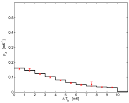
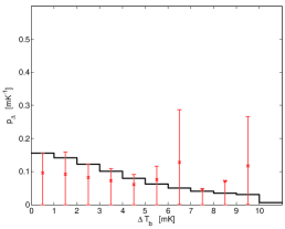
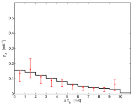
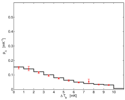
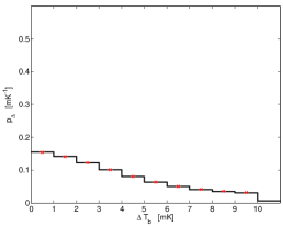
Finally, at a higher redshift when reionization is still in its early stages, measurements are more difficult so we show only the two highest distance bins, 61.4 (Figure 15) and 119.5 Mpc (Figure 16). At this redshift, only MWA/10 errors allow useful constraints on $p_{\Delta}$, in particular giving a reasonable measurement at 119.5 Mpc.

(a) Subfigure 1 list of figures text

(b) Subfigure 1 list of figures text

(c) Subfigure 2 list of figures text

Figure 15: Same as Figure 10 (i.e., $r_{\rm mid}=61.4$ Mpc) but at $z=10.1$.

(a) Subfigure 1 list of figures text

(b) Subfigure 1 list of figures text

(c) Subfigure 2 list of figures text

Figure 16: Same as Figure 15 but for the $r_{\rm mid}=119.5$ Mpc bin.

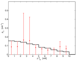
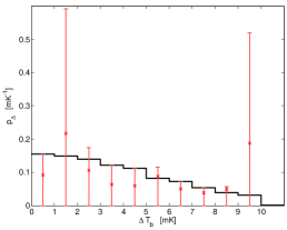
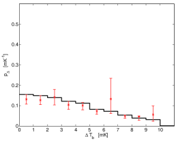
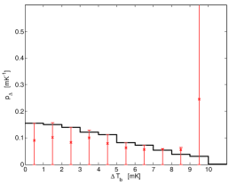
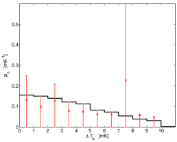
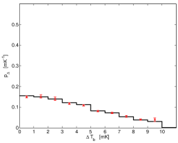
We conclude that with the 10-bin model, one-year MWA observations can give a rough measurement of the difference PDF only at the highest separation, and during mid-to-late reionization. Four-year observations would substantially decrease the errors on the highest separation bin, and give some constraints on the lower, $r_{\rm mid}=61.4$ Mpc bin. However, only with MWA/10 thermal noise, i.e., with next generation radio array experiments, will it be possible to recover the shape of the difference PDF across most distances, and thus directly constrain the ionization correlation length (or bubble size) with few assumptions needed.

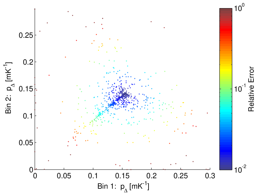
With multiple parameters in the 10-bin model, the results are driven by degeneracies between the probability fit values of various bins. We plot an example of this in Figure 17, for the first two bins out of the ten. Since it is hard to distinguish neighboring bins, a significant fraction of the values lie along a diagonal line that illustrates a strong positive correlation. A few poor fits lie on the axes, since the fit parameters for each $\Delta T_{b}$ bin denote probabilities and were constrained to non-negative values in the chi-squared minimization. Thirty-three fit values (out of 1,000) lie outside the boundaries shown in the figure.

Figure 17: Fits of the first 2 bins in the 10-bin model, at $z=8.2$, with $r_{\rm mid}=61.4$ comoving Mpc, for MWA/2 noise. Bin 1 is $\Delta T=0$ to 1 mK, while Bin 2 is $\Delta T=1$ to 2 mK. We color code the fit values for each of the 1,000 instances of mock observational data by the root-mean-square of the relative errors in Bin 1 and Bin 2. The mean fit and 1-$\sigma$ errors of all 10 bins can be seen in Figure 13b.

4 Conclusions

We have studied the expected errors in reconstructing the difference PDF of the 21-cm brightness temperature during cosmic reionization. We have shown how to perform a maximum likelihood fit to a model of a binned difference PDF, and applied it to mock observational data for a realistic field of view and a range of thermal noise levels.

Previous work shows that the difference PDF during reionization should display a strongly evolving shape that, if measured, can be used to probe both the mean ionization history and the typical size of the ionized bubbles. Early in reionization, the difference PDF still resembles the Gaussian shape driven by density fluctuations, but it later flattens and develops a two-peak structure, including a peak at $\Delta T_{b}=0$ due to jointly-ionized pixel pairs, and a peak at $\Delta T_{b}\sim 10-15$ mK due to the temperature difference between an ionized pixel and one that is still mostly neutral. The difference PDF reaches an asymptotic form at large pair separations (where the two pixels in the pair are essentially independent); the distance below which it substantially changes shape is a measure of the correlation length (of density, early on, and mainly of ionization during the later stages of reionization).

We have found that a conservative approach that attempts only to reconstruct the first bin of the difference PDF (which is related to the ionization correlation function) should yield highly accurate measurements. Even one-year MWA data should suffice for seeing the signature of the end of reionization in the difference PDF, and for probing large separations at earlier times. Four-year data should improve things markedly, typically decreasing errors by about a factor of 4 (rather than the usual 2), since decreased noise helps remove some of the partial degeneracies inherent in what is essentially an attempt to deconvolve the noisy difference PDF. A second generation experiment should be able to probe a wide range of separations during most of the reionization era, assuming that reionization ends at $z\sim 7$ and not much earlier. We note that measuring the 1-bin model (i.e., a single parameter) is qualitatively similar in difficulty to measuring the correlation function (or equivalently the power spectrum), which is essentially equivalent to measuring a single number (the variance) from the difference PDF in each bin of separation distance.

Given these results with a 1-bin model, we have also considered a more ambitious attempt to measure the detailed shape of the difference PDF over ten bins. We found that with the 10-bin model, one-year MWA observations can give a rough measurement of the difference PDF only at the highest separation, and during mid-to-late reionization. Four-year observations can give some improved constraints, but only a second-generation radio array will make it possible to recover the detailed shape of the difference PDF across a range of distances and reionization stages.

We note that while we have only gone up to the bin of separation distance centered at $r=120$ Mpc, it would be useful to measure bins at even larger separations. Theoretically, $p_{\Delta}$ should be pretty much constant with $r$ at such large distances, since the two voxels of a pair are essentially independent of each other, but observationally the number of pairs keeps rising with distance. The total number of pairs in the MWA field of view, given the pixel size of 2.9 Mpc, is $\sim 3\times 10^{15}$ at $z=8$. Thus, the number of pairs available for measuring the large-separation difference PDF is potentially 100 times larger than the value we assumed, which was already high compared to the available numbers at smaller separations. While a measurement of the large-separation difference PDF would not probe correlation functions, it would probe the cosmic mean ionized fraction and, essentially, the one-point PDF (which independently describes each point of the pair) at an exquisite precision.

Now that we have shown that measurements of the difference PDF are quite promising relative to the expected thermal noise, the next challenge is to consider similar statistics in the presence of realistic foreground residuals and other systematic errors. In particular, systematic errors that vary across the field of view might make it in practice difficult to include the just-mentioned wide-separation pairs.

References

- Barkana & Loeb (2008) Barkana R., Loeb A., 2008, MNRAS, 384, 1069
- Bowman, Morales & Hewitt (2009) Bowman J. D., Morales M. F., Hewitt J. N., 2009, ApJ, 695, 183
- Cash (1979) Cash W., 1979, ApJ, 228, 939
- Ciardi & Madau (2003) Ciardi B., Madau P., 2003, ApJ, 596, 1
- Furlanetto, Oh & Briggs (2006) Furlanetto S. R., Oh S. P., Briggs F. H., 2006, Phys. Rep., 433, 181
- Furlanetto, Zaldarriaga & Hernquist (2004) Furlanetto S. R., Zaldarriaga M., Hernquist L., 2004, ApJ, 613, 16
- Gluscevic & Barkana (2010) Gluscevic V., Barkana R., 2010, MNRAS, 408, 2373
- Harker et al. (2010) Harker G. et al., 2010, MNRAS, 405, 2492
- Harker et al. (2009) Harker G. J. A. et al., 2009, MNRAS, 393, 1449
- Ichikawa et al. (2010) Ichikawa K., Barkana R., Iliev I. T., Mellema G., Shapiro P. R., 2010, MNRAS, 406, 2521
- Jacobs et al. (2011) Jacobs D. C. et al., 2011, ApJ, 734, L34
- McQuinn et al. (2007) McQuinn M., Lidz A., Zahn O., Dutta S., Hernquist L., Zaldarriaga M., 2007, MNRAS, 377, 1043
- Mellema et al. (2006) Mellema G., Iliev I. T., Pen U.-L., Shapiro P. R., 2006, MNRAS, 372, 679
- Paciga et al. (2011) Paciga G. et al., 2011, MNRAS, 413, 1174
- Wyithe & Morales (2007) Wyithe J. S. B., Morales M. F., 2007, MNRAS, 379, 1647