Efficient Simulation of Geothermal Processes in Heterogeneous Porous Media based on the Exponential Rosenbrock-Euler and Rosenbrock-type Methods

Abstract

Simulation of geothermal systems is challenging due to coupled physical processes in highly heterogeneous media. Combining the exponential Rosenbrock–Euler and Rosenbrock-type methods with control-volume (two-point flux approximation) space discretizations leads to efficient numerical techniques for simulating geothermal systems. In terms of efficiency and accuracy, the exponential Rosenbrock–Euler time integrator has advantages over standard time-dicretization schemes, which suffer from time-step restrictions or excessive numerical diffusion when advection processes are dominating. Based on linearization of the equation at each time step, we make use of matrix exponentials of the Jacobian from the spatial discretization, which provide the exact solution in time for the linearized equations. This is at the expense of computing the matrix exponentials of the stiff Jacobian matrix, together with propagating a linearized system. However, using a Krylov subspace or Leja points techniques make these computations efficient.

The Rosenbrock-type methods use the appropriate rational functions of the Jacobian from the spatial discretization. The parameters in these schemes are found in consistency with the required order of convergence in time. As a result, these schemes are A-stable and only a few linear systems are solved at each time step. The efficiency of the methods compared to standard time-discretization techniques are demonstrated in numerical examples.

1 Introduction

In the subsurface, producing geothermal systems are characterized by coupled hydraulic, thermal, chemical and mechanical processes. To determine the potential of a geothermal site, and decide optimal production strategies, it is important to understand and quantify these processes. Rigorous mathematical modeling and accurate numerical simulations are essential, but multiple interacting processes acting on different scales leads to challenges in solving the coupled system of equations.

Standard discretization methods include finite element, control-volume and finite difference methods for the space discretization (see [1, 4, 9, 13] and references therein), while standard implicit, explicit or implicit-explicit methods have until recently mostly been used for the discretization in time [36, 37]. Challenges with the discretization are, amongst others, related to severe time-step restrictions associated with explicit methods and excessive numerical diffusion for implicit methods. Furthermore, implicit methods require at each time step the solution of large systems of nonlinear equations, which may lead to bottlenecks in practical computations.

In this paper, we consider a different approach for the temporal discretization based on the Exponential Rosenbrock–Euler Method (EREM) and Rosenbrock-type Methods (ROSM). Exponential integrators have recently been suggested as efficient and robust alternatives for the temporal discretization for several applications (see [8, 17, 41, 44]. Rosenbrock-type methods have been intensively developed in the literature and used in a variety of applications (see [2, 20, 28, 29] and reference therein). However, neither of these approaches have yet found wide-spread use in porous media applications.

The mathematical model discussed, consists of a system of partial differential equations that express conservation of mass and energy. In addition, the model entails phenomenological laws describing processes active in the reservoir, such as Darcy’s law for fluid flow with variable density and viscosity, Fourier’s law of heat conduction, and those describing the relation between fluid properties (nonlinear fluid expansivity and compressibility) and porosity subject to pressure and temperature variations. The resulting system of equations is nonlinear and coupled and requires sophisticated numerical techniques.

Our solution technique is based on a sequential approach, which decouples the mathematical model. An advantage of this approach is that it allows for specialized solvers for unknowns with different characteristics. As the linearized fully coupled matrices are often very poorly conditioned such that small time-steps are required, a carefully chosen sequential approach leads to higher efficiency and accuracy than a simultaneous solution approach if the couplings are not too strong [9]. A finite volume method is applied for the space discretization while the Exponential Rosenbrock–Euler Method and Rosenbrock-type methods are applied to integrate the systems in time based on successive linearizations.

The Exponential Rosenbrock–Euler method is based on the linearization of the ODEs resulting from the space discretization at each time step. The linear part is solved exactly in time up to a given tolerance in the computation of a matrix exponential function of the Jacobian. The nonlinear part is approximated using low-order Taylor expansions. As in all exponential integrator schemes, the expense is the computation of the matrix exponentials of the stiff Jacobian matrix resulting from the spatial discretization. Computing matrix exponentials of stiff matrices is a notorious problem in numerical analysis [33], but new developments for both Léja points and Krylov subspace techniques [3, 22, 40, 41, 45] have led to efficient numerical approaches; see e.g. [5, 8, 17, 41] and references therein. Besides, the method is L-stable, and performs well for super-stiff ODEs.

The Rosenbrock-type methods use the appropriate rational functions of the Jacobian from the spatial discretization. The parameters in these schemes are found in consistency with the required order of convergence in time. As a result these schemes are A-stable (as will be discussed below) and only few linear systems are solved at each time step.

The paper is organized as follows. We present the model equations in Section 2, and the finite volume method for spatial discretization in Section 3, along with temporal discretization schemes. The implementation of the Exponential Rosenbrock-Euler method is discussed in Section 4. In Section 5 we present some numerical examples, which also include simulations for a fractured reservoir, and show comparisons to standard approaches, before we draw conclusions in Section 6.

2 Model equations

We assume single-phase flow of water, which allows the energy equation to be written in terms of temperature. The model equations are given by

$$\left\{\begin{array}[]{l}(1-\phi)\rho_{s}c_{ps}\dfrac{\partial T_{s}}{\partial t}=(1-\phi)\nabla\cdot(\mathbf{k}_{s}\nabla T_{s})+(1-\phi)q_{s}+he(T_{f}-T_{s)}\\ \phi\rho_{f}c_{pf}\dfrac{\partial T_{f}}{\partial t}=\phi\nabla\cdot(\mathbf{k}_{f}\nabla T_{f})-\nabla\cdot(\rho_{f}c_{pf}\mathbf{v}T_{f})+\phi q_{f}+he(T_{s}-T_{f)}\\ \end{array}\right.$$ (3)

(see [11, 34]). The model equations are given in the bounded spatial domain $\Omega\subset\mathbb{R}^{d},\;d={2,3}$, with boundary $\partial\Omega$, and in the time interval is $\left[0,\tau\right]$. Here $\phi$ is the porosity; $he$ is the heat transfer coefficient; $q$ is the heat production; $\rho$ is the density; $c_{p}$ stand for heat capacity; $T$ is the temperature; $\mathbf{k}$ is the thermal conductivity tensor, with the subscripts $f$ and $s$ referring to fluid and rock; and $\mathbf{v}$ is the Darcy velocity given by

$$\mathbf{v}=-\dfrac{\mathbf{K}}{\mu}\left(\nabla p-\rho_{f}\mathbf{g}\right),$$ (4)

where $\mathbf{K}$ is the permeability tensor, $\mu$ is the viscosity, $\mathbf{g}$ is the gravitational acceleration and $p$ the pressure. The mass balance equation for a single-phase fluid is given by

$$\dfrac{\partial\phi\rho_{f}}{\partial t}=-\nabla\cdot(\mathbf{v}\rho_{f})+Q_{f},$$ (5)

where $Q[\text{kg/s}]$ is contribution from a source or sink per time unit. Assuming in equation (5) that the rock is slightly compressible, the porosity is a function of pressure and can be expressed as a linear function, yielding

$$\rho_{f}\dfrac{\partial\phi}{\partial t}+\phi\dfrac{\partial\rho_{f}}{\partial t} = \nabla\cdot\left(\dfrac{\rho_{f}\mathbf{K}}{\mu}\left(\nabla p-\rho_{f}\mathbf{g}\right)\right)+Q_{f},$$ (6)

with

$$\phi=\phi_{0}\left(1+\alpha_{b}(p-p_{0})\right),$$ (7)

where $\phi_{0}$ is the porosity at the initial pressure, $p_{0}$ the initial pressure and $\alpha_{b}$ the bulk vertical compressibility of the porous medium.

Notice that

$$\dfrac{\partial\rho_{f}}{\partial t} = \dfrac{\partial\rho_{f}}{\partial T_{f}}\dfrac{\partial T_{f}}{\partial t}+\dfrac{\partial\rho_{f}}{\partial p}\dfrac{\partial p}{\partial t}$$ (8)

$$= \rho_{f}\left(-\alpha_{f}\dfrac{\partial T_{f}}{\partial t}+\beta_{f}\dfrac{\partial p}{\partial t}\right),$$ (9)

where $\alpha_{f}$ and $\beta_{f}$ are respectively the thermal fluid expansivity and its compressibility defined by

$$\alpha_{f}=-\dfrac{1}{\rho_{f}}\dfrac{\partial\rho_{f}}{\partial T_{f}},\,\;\;\;\;\beta_{f}=\dfrac{1}{\rho_{f}}\dfrac{\partial\rho_{f}}{\partial p}.$$ (10)

Inserting equation (8) and (7) in equation (6) yields

$$-\phi\rho_{f}\alpha_{f}\dfrac{\partial T_{f}}{\partial t}+\rho_{f}\left(\phi\beta_{f}+\phi_{0}\alpha_{b}\right)\dfrac{\partial p}{\partial t} = \nabla\cdot\left(\dfrac{\rho_{f}\mathbf{K}}{\mu}\left(\nabla p-\rho_{f}\mathbf{g}\right)\right)+Q_{f},$$ (11)

The state functions $\mu$,$\rho_{f},\alpha_{f},\beta_{f}$ and $c_{pf}$ can found [15, 19].

The model problem is therefore to find the functions $(T_{s},T_{f},p)$ satisfying the nonlinear equations (3) and (11) subject to (4). Notice if $he\rightarrow\infty$ we have the equilibrium state of the heat with $T_{s}=T_{f}$.

3 Numerical Schemes

3.1 Space discretization

We use the finite volume method[13, 14] on a structured mesh $\mathcal{T}$, with maximum mesh size $h$. We denote by ($\Omega_{i}$) the family of control volumes of mesh $\mathcal{T}$. The finite volume method space discretization consists in:

1. Integrate each equations of (3) and (11) over each control volume $\Omega_{i}$.

2. Use the divergence theorem to convert the volume integral into the surface integral in all divergence terms.

3. Use two-point flux approximations for diffusion heat and flow fluxes [13]

   $$f_{i}^{1}=\int_{\partial\Omega_{i}}\mathbf{n}_{i}\cdot\left(\mathbf{k_{s}}\nabla T_{s}\right)ds,\;\;f_{i}^{2}=\int_{\partial\Omega_{i}}\mathbf{n}_{i}\cdot\left(\mathbf{k_{f}}\nabla T_{f}\right)ds,\;\;$$ (12)

   $$f_{i}^{3}=\int_{\partial\Omega_{i}}\mathbf{n}_{i}\cdot\left(\dfrac{\rho_{f}\mathbf{K}}{\mu}\nabla p\right)ds.$$ (13)

4. Use the standard upwind weighting [13] for the convective (advective) flux

   $$f_{i}^{4}=\int_{\partial\Omega_{i}}\mathbf{n}_{i}\cdot\left(\rho_{f}c_{pf}T_{f}\mathbf{v}\right)ds.\;\;$$ (14)

Here we denote by $\mathbf{n}_{i}$ the unit normal vector to $\partial\Omega_{i}$ outward to $i$ and $ds$ the elementary surface measure. For an edge $\sigma$ of the control volume $i$, $\mathbf{n}_{i,\sigma}$ will denote the unit normal vector to $\sigma$ outward to $\Omega_{i}$.

Let us illustrate the spatial discretization of the second equation of (3) on a structured mesh $\mathcal{T}$ (the two-point flux approximation is sufficient for so-called $\bf K$-orthogonal grids). We denote by $\;\mathcal{E}_{int}$ the set of interior edges of the control volumes of $\mathcal{T}$. For any function $X$, $X_{i}(t)$ denotes the approximation of $X$ at time $t$ at the center of the control volume $\Omega_{i}\in\mathcal{T}$ and $X_{\sigma}(t)$ the approximation of $X$ at time $t$ at the center of the edge $\sigma$. For a control volume $\Omega_{i}\in\mathcal{T}$, we denote by $\mathcal{E}_{i}$ the set of edges of $\Omega_{i}$, $|\Omega_{i}|$ the Lebesgue measure of the control volume $\Omega_{i}\in\mathcal{T}$, $i\mid j$ the edge interface between the control volume $\Omega_{i}$ and the control volume $\Omega_{j}\neq\Omega_{i}$, $d_{i,j}$ the distance between the center of the control volume $\Omega_{i}$ and center of the control volume $\Omega_{j}$, and $d_{i,\sigma}$ the distance between the control volume $\Omega_{i}$ and the edge $\sigma$. Letting $\mathbf{k_{s}}:=\mathbf{k}$, we therefore have

$$f_{i}^{2} = \int_{\partial\Omega_{i}}\mathbf{n}_{i}\cdot\left(\mathbf{k}\nabla T_{f}\right)ds=\underset{\sigma\in\mathcal{E}_{i}}{\sum}f_{i,\sigma}$$

$$f_{i,\sigma}(t) \approx |\sigma|\;k_{i,\sigma}\dfrac{T_{f\sigma}(t)-T_{fi}(t)}{d_{i,\sigma}},\,\,\,\,\,\,\,\,\sigma\in\partial\Omega\$$

$$f_{i,\sigma}(t) \approx -\tau_{\sigma}\left(T_{fj}(t)-T_{fi}(t)\right),\,\,\,\,\,\,\,\,\sigma=i\mid j\in\mathcal{E}_{int}$$

$$\tau_{\sigma} = |\sigma|\dfrac{k_{i,\sigma}k_{j,\sigma}}{k_{i,\sigma}\;d_{i,\sigma}+k_{j,\sigma}d_{j,\sigma}}$$

$$k_{i,\sigma} = |\mathbf{k}_{i}\,\mathbf{n}_{i,\sigma}|,\quad\mathbf{k}_{i}=\dfrac{1}{|\Omega_{i}|}\int_{i}\mathbf{k}(\mathbf{x})d\mathbf{x},$$

These approximations are for interior edges and Dirichlet Boundary condition. For a Neumann boundary condition, $\mathbf{n}_{i}\cdot\left(\mathbf{k}\nabla T_{f}\right)$ is naturally given. In the case of a discrete-fracture model, we make adjustments to the spatial discretization following the approach in [39, 26].

To determine the convective fluxes, we set $X=\rho_{f}c_{pf}T_{f}$. Standard upwind weighting yields

$$f_{i}^{4} = \int_{\partial\Omega_{i}}\mathbf{n}_{i}\cdot\left(\rho_{f}c_{pf}T_{f}\mathbf{v}\right)ds=\underset{\sigma\in\mathcal{E}_{i}}{\sum}\int_{\sigma}\mathbf{n}_{i,\sigma}\cdot X\mathbf{v}ds\approx\underset{\sigma\in\mathcal{E}_{i}}{\sum}v_{i,\sigma}X_{\sigma,+}(t)$$

$$v_{i,\sigma} = \int_{\sigma}\mathbf{n}_{i,\sigma}\mathbf{v}ds$$ (15)

$$X_{\sigma,+}(t) = \left\{\begin{array}[]{l}X_{i}(t)\quad\text{if}\quad v_{i,\sigma}\geqslant 0\\ \newline \\ X_{j}(t)\quad\text{if}\quad v_{i,\sigma}<0\end{array}\right.\;\;\;\;\text{for}\;\;\;\sigma=i\mid j$$ (19)

$$X_{\sigma,+}(t) = \left\{\begin{array}[]{l}X_{i}(t)\quad\text{if}\quad v_{i,\sigma}\geqslant 0\\ \newline \\ X_{\sigma}(t)\quad\text{if}\quad v_{i,\sigma}<0\end{array}\right.\;\;\text{for}\;\;\sigma\in\mathcal{E}_{i}\cap\partial\Omega.$$ (23)

Reorganizing these space approximations yield the following system of ODEs

$$\left\{\begin{array}[]{rcl}\dfrac{dT_{s}^{h}}{dt}&=&G_{1}(T_{s}^{h},T_{f}^{h},t)\\ \newline \\ \dfrac{dT_{s}^{h}}{dt}&=&G_{2}(T_{s}^{h},T_{f}^{h},p_{h},t)\\ \newline \\ \dfrac{dp_{h}}{dt}&=&G_{3}(p_{h},T_{f}^{h},t)+\dfrac{(\phi\alpha_{f})(T_{f}^{h},p_{h})}{(\phi\beta_{f}+\phi_{0}\alpha_{b})(T_{f}^{h},p_{h})}\cdot\dfrac{dT_{s}^{h}}{dt}\end{array}\right.$$ (29)

$$\Leftrightarrow\left\{\begin{array}[]{l}\dfrac{dT_{h}}{dt}=G(T^{h},p_{h},t)\\ \newline \\ \dfrac{dp_{h}}{dt}=G_{3}(p_{h},T_{f}^{h},t)+\dfrac{(\phi\alpha_{f})(T_{f}^{h},p_{h})}{(\phi\beta_{f}+\phi_{0}\alpha_{b})(T_{f}^{h},p_{h})}\cdot G_{2}(T_{s}^{h},T_{f}^{h},p_{h},t)\\ \newline \\ G(T^{h},p_{h},t)=(G_{1}(T_{s}^{h},T_{f}^{h},t),G_{2}(T_{s}^{h},T_{f}^{h},p_{h},t))^{T}\\ \newline \\ T_{h}=(T_{s}^{h},T_{f}^{h})^{T}\approx(T_{s},T_{f})^{T}.\end{array}\right.$$ (37)

For a given initial pressure $p_{h}(0)$, with corresponding initial velocity $\mathbf{v}_{h}(0)$) and initial temperature $T_{h}(0)$, the technique used in the paper consists in solving successively the systems

$$\left\{\begin{array}[]{l}\dfrac{dT_{h}}{dt}=G(T^{h},p_{h},t)\\ \newline \\ T_{h}(0),\,p_{h}(0)\;\;\;\textbf{given}\end{array}\right.$$ (41)

and

$$\left\{\begin{array}[]{l}\dfrac{dp_{h}}{dt}=G_{3}(p_{h},T_{f}^{h},t)+\dfrac{(\phi\alpha_{f})(T_{f}^{h},p_{h})}{(\phi\beta_{f}+\phi_{0}\alpha_{b})(T_{f}^{h},p_{h})}\cdot G_{2}(T_{s}^{h},T_{f}^{h},p_{h},t)=G_{4}(T_{h}^{h},p_{h},t)\\ \newline \\ T_{h}(0),\,p_{h}(0)\;\;\;\textbf{given}.\end{array}\right.$$ (45)

The ODEs (37) is usualy stiff since the smaller absolute value of the eigenvalues of the Jacobian matrix is usually closed to zero.

3.2 Time discretizations

We now present our numerical methods for the ODEs (37) based on the sequential approach. Considering a sequential solution approach, we start by presenting low order time discretization schemes and their stability properties before we give some higher order schemes.

3.2.1 $\theta$-Euler Schemes

We briefly describe the standard integrators that will be used for comparison with Exponential Rosenbrock-Euler method and Rosenbrock-type methods. Consider the ODEs (41) and (45) within the interval $[0,\tau],\,\tau>0$. Given a time-step $\tau_{n}$, applying the $\theta-$Euler scheme with respect to the function $T_{h}$ in the ODEs (41) yields

$$\left\{\begin{array}[]{l}\dfrac{T_{h}^{n+1}-T_{h}^{n}}{\tau_{n}}=\theta G(T_{h}^{n+1},p_{h}^{n},t_{n+1})+(1-\theta)G(T_{h}^{n},p_{h}^{n},t_{n})\\ \newline \\ T_{h}(0)=T_{h}^{0},\;\;\;\;\;0\leq\theta\leq 1.\end{array}\right.$$ (49)

For $\theta\neq 0$ the scheme is implicit and given the approximate solutions $T_{h}^{n}$ and $p_{h}^{n}$ at time $t_{n}$, the solution $T_{h}^{n+1}$ at time $t_{n+1}$ is obtained by solving the nonlinear equation

$$\mathcal{F}(X)=X-\tau_{n}\theta G(X,p_{h}^{n},t_{n+1})-\tau_{n}(1-\theta)G(T_{h}^{n},p_{h}^{n},t_{n})-T_{h}^{n}=0,\,\,\,X=T_{h}^{n+1},$$ (50)

which is solved using the Newton method. For efficiency, all linear systems are solved using the Matlab function bicgstab with ILU(0) preconditioners with no fill-in, which are updated at each time step.

To solve the ODEs (45) we apply again the $\theta$-Euler method, but with respect to $p_{h}$, yielding

$$\left\{\begin{array}[]{l}\dfrac{p_{h}^{n+1}-p_{h}^{n}}{\tau_{n}}=\theta G_{4}(T_{h}^{n+1},p_{h}^{n},t_{n+1})+(1-\theta)G_{4}(T_{h}^{n},p_{h}^{n},t_{n})\\ \newline \\ p_{h}(0)=p_{h}^{0}.\end{array}\right.$$ (54)

For $\theta=1/2$ the $\theta$-Euler scheme is second order in time, and for $\theta\neq\frac{1}{2}$ the scheme is first order in time. In this paper, the standard sequential approach to solve the ODEs (29) consists of applying successively the schemes (49) and (54).

3.2.2 Exponential Rosenbrock-Euler Method and Rosenbrock-type Methods

To introduce the Exponential Euler-Rosenbrock Method (also called Exponential Euler Method), let us first consider the following system of ODEs

$$\left\{\begin{array}[]{l}\dfrac{d\mathbf{y}}{dt}=\mathbf{L}\mathbf{y}+\mathbf{g}(\mathbf{y},t),\;\;\;\;\ t\in[0,\tau]\\ \mathbf{y}(0)=\mathbf{y}_{0},\end{array}\right.$$ (57)

which appear after spatial discretisation of semilinear parabolic PDEs. Here $\mathbf{L}$ is a stiff matrix and $\mathbf{g}$ a nonlinear function. This allows us to write the exact solution of (57) as

$$\mathbf{y}(t_{n})=e^{t_{n}\mathbf{L}}\mathbf{y}_{0}+\int_{0}^{t_{n}}e^{(t_{n}-s)\mathbf{L}}\mathbf{g}(\mathbf{y}(s),s)ds.$$

Given the exact solution at the time $t_{n}$, we can construct the corresponding solution at $t_{n+1}$ as

$$\mathbf{y}(t_{n+1}) = e^{\tau_{n}\mathbf{L}}\mathbf{y}(t_{n})+\int_{0}^{\tau_{n}}e^{(\tau_{n}-s)\mathbf{L}}\mathbf{g}(\mathbf{y}(t_{n}+s),s+t_{n})ds,$$ (58)

$$\tau_{n} = t_{n+1}-t_{n}.$$ (59)

Note that the expression in (58) is still an exact solution. The idea behind Exponential Time Differencing (ETD) is to approximate $\mathbf{g}(\mathbf{y}(t_{n}+s),t_{n}+s)$ by a suitable polynomial [12]. The simplest case is when $\mathbf{g}(\mathbf{y}(t_{n}+s),t_{n}+s)$ is approximated by the constant $\mathbf{g}(\mathbf{y}(t_{n}),t_{n})$. The corresponding (ETD1) scheme is given by

$$\mathbf{y}^{n+1}=e^{\tau\mathbf{L}}\mathbf{y}^{n}+\tau_{n}\varphi_{1}(\tau_{n}\mathbf{L})\mathbf{g}(\mathbf{y}^{n},t_{n}),$$ (60)

where

$$\varphi_{1}(A)=\underset{i=1}{\sum^{\infty}}\dfrac{A^{i-1}}{i!}=A^{-1}(e^{A}-I)\;\;(\text{if $A$ is invertible}).$$

Note that the ETD1 scheme in (60) can be rewritten as

$$\mathbf{y}^{n+1}=\mathbf{y}^{n}+\tau_{n}\varphi_{1}(\tau_{n}\mathbf{L})(\mathbf{L}\mathbf{y}^{n}+\mathbf{g}(\mathbf{y}^{n},t_{n})).$$ (61)

This new expression has the advantage that it is computationally more efficient as only one matrix exponential function needs to be evaluated at each step.

Recently, the ETD1 scheme was applied to advection-dominated reactive transport in heterogeneous porous media [41, 45]. For this problem, a rigorous convergence proof is established for the case of a finite volume discretization in space [41, 42]. In these works, it was observed that the exponential methods were generally more accurate and efficient than standard implicit methods.

As our systems (41) and (45) are nonlinear, we need to linearize before applying the ETD1 scheme. Consider the system the ODEs (41). For simplicity we assume that it is autonomous

$$\left\{\begin{array}[]{l}\dfrac{dT_{h}}{dt}=G(T_{h},p_{h})\;\;\;\;\;\;\;\newline \\ T_{h}(0)=T_{0}.\end{array}\right.$$ (64)

Let $T_{h}^{n}$ and $p_{h}^{n}$ be the numerical approximations of the exact solutions $T(t_{n})$ and $p(t_{n})$. To obtain the numerical approximation $T_{h}^{n+1}$ of the exact solution $T(t_{n+1})$, we linearize $G(T_{h},p_{h}^{n})$ at $T_{h}^{n}$ and obtain the following semilinear ODEs

$$\dfrac{dT_{h}}{dt} = \mathbf{J}_{n}T_{h}(t)+\mathbf{g}(T_{h}(t),p_{h}^{n})\;\;\;t_{n}\leq t\leq t_{n+1},$$ (65)

where $\mathbf{J}_{n}$ denotes the Jacobian of the function $G$ respect to $T_{h}$ and $\mathbf{g}$ the remainder given by

$$\mathbf{J}_{n}=D_{T_{h}}G(T_{h}^{n},p_{h}^{n}),\;\;\;\;\mathbf{g}(T_{h}(t),p_{h}^{n})=G(T_{h}(t),p_{h}^{n})-\mathbf{J}_{n}T_{h}(t).$$ (66)

Applying the ETD1 scheme to (65) yields

$$T_{h}^{n+1}=T_{h}^{n}+\tau_{n}\varphi_{1}(\tau_{n}\mathbf{J}_{n})G(T_{h}^{n},p_{h}^{n}),\;\;\;\tau_{n}=t_{n+1}-t_{n}.$$ (67)

This scheme, called the Exponential Rosenbrock-Euler method (EREM)[5] (or the Exponential Euler method (EEM)) has been reinvented in different names (see references in [8]).

The EREM scheme is second order in time [5, 8] for autonomous problems. To deal with non-autonomous problems, while conserving the second order accuracy of EERM scheme, it must first be converted to autonomous problems. The corresponding version is given in the next section by equation(86).

The scheme (67) contains the exponential matrix function $\varphi_{1}$. To obtain the simplest Rosenbrock-type methods, the exponential function is approximated by the following rational function

$$\varphi_{1}(\tau_{n}\mathbf{J}_{n})\approx\left(\mathbf{I}-\tau_{n}\gamma\mathbf{J}_{n}\right)^{-1},$$ (68)

where $\gamma>0$ is a parameter. For a given parameter $\gamma>0$, using the approximation (68) in equation (67), the corresponding Rosenbrock-type Method (also called linear implicit methods) is given by

$$T_{h}^{n+1}=T_{h}^{n}+\tau_{n}\left(\mathbf{I}-\tau_{n}\gamma\mathbf{J}_{n}\right)^{-1}G(T_{h}^{n},p_{h}^{n}).\;$$ (69)

For the parameter $\gamma=1/2$, the corresponding Rosenbrock-type Method is order two in time for regular solutions and order 1 if $\gamma\neq 1/2$.

To solve the ODEs (45) we apply again the EREM scheme or the Rosenbrock-type method (69), but with respect to $p_{h}$, which yields respectively

$$\left\{\begin{array}[]{l}p_{h}^{n+1}=p_{h}^{n}+\tau_{n}\varphi_{1}(\tau_{n}\mathcal{J}_{n})G_{4}(T_{h}^{n},p_{h}^{n}),\\ \newline \\ \mathcal{J}_{n}=D_{p_{h}}G_{4}(T_{h}^{n},p_{h}^{n}),\end{array}\right.$$ (73)

and

$$p_{h}^{n+1}=p_{h}^{n}+\tau_{n}\left(\mathbf{I}-\tau_{n}\gamma\mathcal{J}_{n}\right)^{-1}G_{4}(T_{h}^{n},p_{h}^{n}).$$ (74)

As with $\theta-$Euler methods, the sequential approaches with the Exponential Rosenbrock-Euler method and Rosenbrock-type methods proposed in this paper consists in solving the ODEs (29) by applying successively the schemes (67) and (69) to the ODEs (41) and the schemes (73) and (74) to the ODEs (45).

The sequential technique presented is the so called Trotter splitting and is generally first order accurate[31, p. 7]. The alternative technique is the so called Strang splitting which consists to apply the schemes (67) and (69) to the ODEs (41) with time step $\dfrac{\tau_{n}}{2}$, afterward apply the schemes (73) and (74) to the ODEs (45) with time step $\tau_{n}$ and then apply again the schemes (67) and (69) to the ODEs (41) with time step $\dfrac{\tau_{n}}{2}$. Strang splitting is formally second -order accurate in time for sufficiently smooth solution [31, p. 7]. We can obviously observe that this approach is less efficient than Trotter splitting. Trotter splitting and Strang splitting are called multiplicative operator splittings.

In the sequel, sequential approach will mean Trotter splitting.

3.2.3 Stability properties of numerical schemes and higher order Rosenbrock-type methods

One of the important features of any numerical scheme is its stability properties. Our goal here is to study the stability properties of the schemes presented in the previous section and high order Rosenbrock-type methods. A special interest will be given to two Rosenbrock-type methods of order two and three because of their good stability properties. In applying the high order Rosenbrock-type methods, we will use the previously presented sequential approaches to solve the ODEs (41) and (45).

Consider the following ODEs

$$\left\{\begin{array}[]{l}\dfrac{d\mathbf{y}}{dt}=\mathbf{f}(\mathbf{y},t),\;\;\;\;\ t\in[0,\tau]\\ \mathbf{y}(0)=\mathbf{y}_{0},\end{array}\right.$$ (77)

where $\mathbf{f}$ is nonlinear function. The corresponding $\theta-$Euler scheme is given by

$$\left\{\begin{array}[]{l}\dfrac{\mathbf{y}^{n+1}-\mathbf{y}^{n}}{\tau_{n}}=\theta\mathbf{f}(\mathbf{y}^{n+1},t_{n+1})+(1-\theta)\mathbf{f}(\mathbf{y}^{n},t_{n})\\ \newline \\ \mathbf{y}(0)=\mathbf{y}_{0}\;\;\;\;\;0\leq\theta\leq 1.\end{array}\right.$$ (81)

Note that the exponential Rosenbrock–Euler method presented in the previous section is for autonomous ODEs. Before applying it to non-autonomous system (77), transformation $\hat{\mathbf{y}}=\left(\mathbf{y},t\right)^{T}$ must be performed to obtain autonomous ODEs. Given the numerical solution $\hat{\mathbf{y}}^{n}=(\mathbf{y}^{n},t_{n})^{T}$, the linearization equation leading to $\hat{\mathbf{y}}^{n+1}$ is given by

$$\hat{\mathbf{y}}^{\prime}(t)=\left[\begin{array}[]{c}\mathbf{y}^{\prime}(t)\\ t^{\prime}\end{array}\right] = \left[\begin{array}[]{cc}D_{\mathbf{y}}\mathbf{f}(\mathbf{y}^{n},t_{n})&D_{t}\mathbf{f}(\mathbf{y}^{n},t_{n})\\ 0&0\\ \end{array}\right]\left[\begin{array}[]{c}\mathbf{y}(t)\\ t\end{array}\right]+\left[\begin{array}[]{c}\mathbf{g}_{n}(\mathbf{y}(t),t)\\ 1\end{array}\right]\newline$$

$$\mathbf{g}_{n}(\mathbf{y}(t),t) = \mathbf{f}(\mathbf{y}(t),t)-D_{\mathbf{y}}\mathbf{f}(\mathbf{y}^{n},t_{n})\mathbf{y}(t)-D_{t}\mathbf{f}\,t.$$

Using this transformation and [5, Lemma 1], the corresponding EREM scheme for non-autonomous system is given by

$$\left\{\begin{array}[]{l}\mathbf{y}^{n+1}=\mathbf{y}^{n}+\tau_{n}\varphi_{1}(\tau_{n}\mathcal{J}_{n})\mathbf{f}(\mathbf{y}^{n},t_{n})+\tau_{n}^{2}\varphi_{2}(\tau_{n}\mathcal{J}_{n})D_{t}\mathbf{f}(\mathbf{y}^{n},t_{n})\\ \newline \\ \mathcal{J}_{n}=D_{\mathbf{y}}\mathbf{f}(\mathbf{y}^{n},t_{n}).\end{array}\right.$$ (86)

The exponential functions $\varphi_{i}$ are defined by

$$\varphi_{i}(z)=\int_{0}^{1}e^{(1-s)z}\dfrac{s^{i-1}}{(i-1)!}ds,\qquad\qquad\qquad\,\,\,\,i\geq 1.$$ (87)

These functions satisfy the recurrence relations

$$\varphi_{i}(z)=\dfrac{\varphi_{i-1}(z)-\varphi_{i-1}(0)}{z},\;\,\;\;\,\,\,\,\varphi_{0}=e^{z}.$$ (88)

The corresponding lower order Rosenbrock-type methods is given by

$$\mathbf{y}^{n+1}=\mathbf{y}^{n}+\tau_{n}\left(\mathbf{I}-\tau_{n}\gamma\mathcal{J}_{n}\right)^{-1}\left[\mathbf{f}(\mathbf{y}^{n},t_{n})+\gamma\tau_{n}D_{t}\mathbf{f}(\mathbf{y}^{n},t_{n})\right].$$ (89)

In order to study their stability properties, we apply the $\theta-$Euler, EREM and ROSM schemes to the linear ODEs $\mathbf{y}^{\prime}=\lambda\mathbf{y}$ with constant time step $\Delta t$. We therefore have

$$\mathbf{y}^{n+1}=R(z)\mathbf{y}^{n},\,\,\,\ z=\Delta t\lambda\,$$ (90)

where $R(z)=\dfrac{1+z(1-\theta)}{1-\theta z}$ for the $\theta-$Euler scheme, $R(z)=\exp{(z)}$ for the EREM scheme and $R(z)=\dfrac{1+z(1-\gamma)}{1-\gamma z}$ for the ROSM scheme.

The function $R(z)$ is called the stability function of the method. The set

$$S=\left\{z\in\mathbb{C},\,\,\,\ |R(z)|\leq 1\right\}$$

is called the stability domain of the method. A numerical method is A -stable if its stability domain $S$ satisfies

$$S\supset\mathbb{C}^{-}=\left\{z\in\mathbb{C},\,\,\,\ \text{Re}\,z\leq 0\right\}.$$

Let us study the A-stability of the $\theta-$Euler. Let $z=x+iy\in\mathbb{C}^{-}$, we have

$$|R(z)|\leq 1 \Leftrightarrow |1+(1-\theta)z|\leq|1-\theta z|$$

$$\Leftrightarrow (1+(1-\theta)x)^{2}+((1-\theta)y)^{2}\leq((1-\theta)x)^{2}+(\theta y)^{2}$$

$$\Leftrightarrow (1-2\theta)(x^{2}+y^{2})+2x\leq 0.$$

We can therefore observe that the $\theta-$Euler scheme is A -stable if

$$1-2\theta\leq 0\Leftrightarrow\theta\geq 1/2,$$

ROSM scheme is A -stable if $\gamma\geq 1/2$ and EREM scheme is A -stable.

A-stability is not the whole answer to the problem of stiff equations, excellent numerical methods for super-stiff equations would be L-stable.

Numerical methods are L-stable if they are A-stable and in addition (see [20])

$$\underset{z\rightarrow-\infty}{\lim}|R(z)|=0.$$

We can observe that the $\theta-$Euler scheme is L-stable if $\theta=1$, the ROSM scheme is L-stable if $\gamma=1$ and the EREM scheme is L-stable.

In the sequel we will use the ROSM schemes with $\gamma=1$ and $\gamma=1/2$, which will be denoted respectively by ROSM$(1)$ and ROSM$(1/2)$.

The s-stage Rosenbrock-type methods for the ODE (77) are given by

$$\left\{\begin{array}[]{l}\left(\dfrac{1}{\tau_{n}\gamma}\mathbf{I}-\mathcal{J}_{n}\right)\mathbf{k}_{ni}=\mathbf{f}(\mathbf{y}_{n}+\underset{j=1}{\sum^{i-1}}a_{ij}\mathbf{k}_{nj},t_{n}+\alpha_{i}\tau_{n})-\underset{j=1}{\sum^{i-1}}\dfrac{c_{ij}}{\tau_{n}}\mathbf{k}_{nj}\\ \qquad\qquad\qquad\qquad+\tau_{n}\gamma_{i}D_{t}\mathbf{f}(\mathbf{y}^{n},t_{n})\,\,\,\,\,\,\,i=1,\cdots,s\\ \newline \\ \qquad\qquad\quad\mathbf{y}^{n+1}=\mathbf{y}^{n}+\underset{i=1}{\sum^{s}}b_{i}\mathbf{k}_{ni}\\ \newline \\ \qquad\qquad\quad\mathbf{y}_{1}^{n+1}=\mathbf{y}^{n}+\underset{i=1}{\sum^{s}}\hat{b}_{i}\mathbf{k}_{ni}.\end{array}\right.$$ (97)

The coefficients $a_{ij},c_{ij},\alpha_{i},\gamma,\gamma_{i},b_{i}$ are obtained by using the consistency conditions required to achieve the desirable order of convergence $p$ in time. Different ways to find these coefficients are presented in the literature (see [2, 20, 28, 29] and references therein). The approximation $\mathbf{y}_{1}^{n+1}$ is called an embedded approximation associated to the s-stage Rosenbrock-type approximation $\mathbf{y}^{n+1}$ and is used to control the local errors for adaptivity purpose. The coefficients $\hat{b}_{i}$ are determined using the consistency conditions such that the embedded approximation is order $p-1$. In this work, we use the second order scheme ROS2(1), where the coefficients are given in Table 1, and also the third order scheme denoted ROS3p in [29], which uses additional conditions to avoid order reduction (see Table 2).

The ROS2(1) scheme is L-stable and the ROS3p scheme is A-stable (see [28]).

$\gamma=1.707106781186547e^{+00}$
$a_{11}=0$	$c_{11}=5.857864376269050e^{-01}$
$a_{21}=5.857864376269050e^{-01}$	$c_{21}=1.171572875253810e^{+00}$
$a_{22}=0$	$c_{22}=5.857864376269050e^{-01}$
$\gamma_{1}=1.707106781186547e^{+00}$	$\alpha_{1}=0$
$\gamma_{2}=-1.707106781186547e^{+00}$	$\alpha_{2}=1$
$b_{1}=8.786796564403575e^{-01}$	$\hat{b}_{1}=5.857864376269050e^{-01}$
$b_{2}=2.928932188134525e^{-01}$	$\hat{b}_{2}=0$

Table 1: Coefficients of the ROS2(1) scheme from [28].

$\gamma=7.886751345948129e^{-01}$
$a_{11}=0$	$c_{11}=1.267949192431123e^{+00}$
$a_{21}=1.267949192431123e^{+00}$	$c_{21}=1.607695154586736e^{+00}$
$a_{22}=0$	$c_{22}=1.267949192431123e^{+00}$
$a_{31}=1.267949192431123e^{+00}$	$c_{31}=3.464101615137755e^{+00}$
$a_{32}=0$	$c_{32}=1.732050807568877e^{+00}$
$a_{33}=0$	$c_{33}=1.267949192431123e^{+00}$
$\gamma_{1}=7.886751345948129e^{-01}$	$\alpha_{1}=0$
$\gamma_{2}=-2.113248654051871e^{-01}$	$\alpha_{2}=1$
$\gamma_{3}=-1.077350269189626e^{+00}$	$\alpha_{3}=1$
$b_{1}=2$	$\hat{b}_{1}=2.113248654051871e^{+00}$
$b_{2}=5.773502691896258e^{-01}$	$\hat{b}_{2}=1$
$b_{3}=4.226497308103742e^{-01}$	$\hat{b}_{3}=4.226497308103742e^{-01}$

Table 2: Coefficients of the ROS3p scheme from [28, 29].

The implementation of Rosenbrock-type schemes is straightforward as there are no nonlinear equations to solve at each time step. For efficiency, all linear systems are solved using the Matlab function bicgstab with ILU(0) preconditioners with no fill-in. The time step adaptivity can be performed using the standard error control and the step size prediction as in [20, pp.112] with an appropriate norm of $\mathbf{y}^{n+1}-\mathbf{y}_{1}^{n+1}$.

4 Implementation of Exponential Rosenbrock-Euler Method

The key element in all exponential integrator schemes is the computation of the matrix exponential functions, the so called $\varphi_{i}-$ functions. There are many techniques available for that task[23]. Standard Padé approximation compute at every time step the whole matrix exponential functions and are therefore memory and time consuming for large problems. Krylov subspace technique and the real fast Leja points technique are proved to be efficient for this computation for large systems [3, 8, 17, 22, 40, 41]. Let us summarize these techniques while solving ODE (77) with the EREM scheme.

4.1 Krylov subspace technique

The main idea of the Krylov subspace technique is to approximate the action of the exponential matrix function $\varphi_{i}(\tau_{n}\mathcal{J}_{n})$ on a vector $\mathbf{v}$ by projection onto a small Krylov subspace $K_{m}=\text{span}\left\{\mathbf{v},\mathcal{J}_{n}\mathbf{v},\ldots,\mathcal{J}_{n}^{m-1}\mathbf{v}\right\}$ [40]. The approximation is formed using an orthonormal basis of $\mathbf{V}_{m}=\left[\mathbf{v}_{1},\mathbf{v}_{2},\ldots,\mathbf{v}_{m}\right]$ of the Krylov subspace $K_{m}$ and of its completion $\mathbf{V}_{m+1}=\left[\mathbf{V}_{m},\mathbf{v}_{m+1}\right]$. The basis is found by Arnoldi iteration, which uses stabilized Gram-Schmidt to produce a sequence of vectors that span the Krylov subspace (see Algorithm 1).

Let $\mathbf{e}_{i}^{j}$ be the $i^{\textrm{th}}$ standard basis vector of $\mathbb{R}^{j}$. We approximate $\varphi_{i}(\tau_{n}\,\mathcal{J}_{n})\mathbf{v}$ by

$$\varphi_{i}(\tau_{n}\,\mathcal{J}_{n})\mathbf{v} \approx \|\mathbf{v}\|_{2}\mathbf{V}_{m+1}\varphi_{i}(\tau_{n}\,\overline{\mathbf{H}}_{m+1})\mathbf{e}_{1}^{m+1}$$ (98)

with

$$\overline{\mathbf{H}}_{m+1}=\left(\begin{array}[]{cc}\mathbf{H}_{m}&\b{0}\\ 0,\cdots,0,h_{m+1,m}&0\end{array}\right)\qquad\text{where}\qquad\mathbf{H}_{m}=\mathbf{V}_{m}^{T}\mathcal{J}_{n}\mathbf{V}_{m}=[h_{i,j}].$$

The coefficient $h_{m+1,m}$ is recovered in the last iteration of Arnoldi’s iteration in Algorithm 1. We denote by $\|.\|_{2}$ the standard Euclidan norm. The approximation (98) is the first two terms of the expansion given in [40, Theorem 2].

1:  Initialise: $\mathbf{v}_{1}=\dfrac{\mathbf{v}}{\|\mathbf{v}\|_{2}}$ {normalisation}

2:  for $j=1\cdots m$ do

3:     $\mathbf{w}=\mathcal{J}\mathbf{v}_{j}$

4:     for $i=1\cdots j$ do

5:        $h_{i,j}=\mathbf{w}^{T}\mathbf{v}_{i}$ {compute inner product to build elements of the matrix $\mathbf{H}$}

6:        $\mathbf{w}=\mathbf{w}-h_{i,j}\mathbf{v}_{i}$ {Gram–Schmidt process}

7:     end for

8:     $h_{j+1,j}=\|\mathbf{w}\|_{2}$

9:     $\mathbf{v}_{j+1}=\dfrac{\mathbf{w}}{\|\mathbf{w}\|_{2}}$ {normalisation}

10:  end for

Algorithm 1 : Arnoldi’s algorithm

For a small Krylov subspace (i.e, $m$ is small) a standard Padé approximation can be used to compute $\varphi_{i}(\tau_{n}\overline{\mathbf{H}}_{m+1})$, but an efficient way used in  [40] is to recover $\varphi_{i}(\tau_{n}\overline{\mathbf{H}}_{m+1})\mathbf{e}_{1}^{m+1}$ directly from the Padé approximation of the exponential of a matrix related to $\mathbf{H}_{m}$.

Notice that this implementation can be done without explicit computation of the Jacobian matrix $\mathcal{J}_{n}$ as the Krylov subspace $K_{m}$ can be formed by using the following approximations

$$\mathcal{J}_{n}\mathbf{v} \approx \dfrac{\mathbf{f}(\mathbf{y}^{n}+\epsilon\mathbf{v},t_{n})-\mathbf{f}(\mathbf{y}^{n},t_{n})}{\epsilon}$$

or

$$\mathcal{J}_{n}\mathbf{v} \approx \dfrac{\mathbf{f}(\mathbf{y}^{n}+\epsilon\mathbf{v},t_{n})-\mathbf{f}(\mathbf{y}^{n}-\epsilon\mathbf{v},t_{n})}{\epsilon},$$

for a suitably chosen perturbation of $\epsilon$ (see [27]), while solving the ODE (77). These approximations prove that the Exponential Rosenbrock-Euler scheme with the Krylov subspace technique can be implemented using the free Jacobian technique. The implementations in Expokit [40] (for function $\varphi_{1}$) and in [35] use the truncation error in the approximation (98) to build the local error estimates (see [40, Theorem 2]). The time step subdivisions depend on the given tolerance and the local errors.

4.2 The real fast Léja point technique

This technique has been successfully applied to the nonlinear advection diffusion-reaction-equation in [3, 5, 7, 32, 41, 45] where advection plays a key role. We will used it to solve the temperature equation (41). The key points of this method are as follows: For a given vector $\mathbf{v}$, real fast Léja points approximate $\varphi_{i}(\tau_{n}\,\mathcal{J}_{n})\mathbf{v}$ by $P_{m}(\tau_{n}\,\mathcal{J}_{n})\mathbf{v}$, where $P_{m}$ is an interpolation polynomial of degree $m$ of $\varphi_{i}$ at the sequence of points $\left\{\xi_{i}\right\}_{i=0}^{m}$ called spectral real fast Léja points. These points $\left\{\xi_{i}\right\}_{i=0}^{m}$ belong to the spectral focal interval $\left[\alpha,\beta\right]$ of the matrix $\tau_{n}\mathcal{J}_{n}$, i.e. the focal interval of the smaller ellipse containing all the eigenvalues of $\tau_{n}\,\mathcal{J}_{n}$. This spectral interval can be estimated by the well known Gershgorin circle theorem [46]. It has been shown that as the degree of the polynomial increases, and hence the number of Léja points increases, superlinear convergence is achieved [7]; i.e.,

$$\underset{m\rightarrow\infty}{\lim}\|\varphi_{i}(\tau_{n}\mathcal{J}_{n})\mathbf{v}-P_{m}(\tau_{n}\,\mathcal{J}_{n})\mathbf{v}\|_{2}^{1/m}=0.$$ (99)

Set $\xi_{0}=\beta$, the sequence of fast Léja points is generated by

$$\underset{k=0}{\prod^{j-1}}|\xi_{j}-\xi_{k}|=\underset{\xi\in\left[\alpha,\beta\right]}{\max}\underset{k=0}{\prod^{j-1}}\mid\xi-\xi_{k}\mid\quad j=1,2,3,\cdots.$$ (100)

Given the Newton’s form of the interpolating polynomial, $P_{m}$ is given by

$$P_{m}(z)=\varphi_{i}\left[\xi_{0}\right]+\underset{j=1}{\sum^{m}}\varphi_{i}\left[\xi_{0},\xi_{1},\cdots,\xi_{j}\right]\underset{k=0}{\prod^{j-1}}\left(z-\xi_{k}\right)$$ (101)

where the divided differences $\varphi_{i}[\bullet]$ are defined recursively by

$$\left\{\begin{array}[]{l}d_{0}=\varphi_{i}\left[\xi_{0}\right]:=\varphi_{i}(\xi_{0}),\;\;d_{1}=\varphi_{i}\left[\xi_{0},\xi_{1}\right]:=\dfrac{\varphi_{i}\left[\xi_{1}\right]-\varphi_{i}\left[\xi_{0}\right]}{\xi_{1}-\xi_{0}}.\\ d_{i}=\varphi_{i}\left[\xi_{0},\xi_{1},\cdots,\xi_{i}\right]=\dfrac{\varphi_{i}\left[\xi_{0},\xi_{1},\cdots,\xi_{i-2},\xi_{i}\right]-\varphi_{i}\left[\xi_{0},\xi_{1},\cdots,\xi_{i-2},\xi_{i-1}\right]}{x_{i}-x_{i-1}}.\end{array}\right.$$ (104)

Due to cancelation errors, this standard procedure cannot produce accurate divided differences with magnitude smaller than machine precision.

It can be shown [38] that the divided differences of a function $f(c+\gamma\xi),\,c=(\alpha+\beta)/2,\,\gamma=(\beta-\alpha)/4$ of the independent variable $\xi$ at the points $\left\{\xi_{i}\right\}_{i=0}^{m}\subset[-2,2]$ are the first column of the matrix function $f(\mathbf{L}_{m})$, where

$$\mathbf{L}_{m}=\tau_{n}\left(c\mathbf{I}_{m+1}+\gamma\mathbf{\widehat{L}}_{m}\right),\;\;\;\mathbf{\widehat{L}}_{m}=\left(\begin{array}[]{cccccc}\xi_{0}&&&&&\\ 1&\xi_{1}&&&&\\ &1&\ddots&&&\\ &&\ddots&\ddots&&\\ &&&\ddots&\ddots\\ &&&&1&\xi_{m}\\ \end{array}\right).$$

Here $\mathbf{I}_{m+1}$ is the identity matrix. To compute $(d_{i})_{0}^{m}=\varphi_{i}(\mathbf{L}_{m})e_{1}^{m+1}$, where $e_{1}^{m+1}$ is the first standard basis vector of $\mathbb{R}^{m+1}$, we apply Taylor expansion of order $p$ with scaling and squaring or Padé approximation [40, 41]. The interest of the Newton interpolation comes from the fact that the approximation with a polynomial of degree $m$ is directly obtained from the approximation with a polynomial of degree $m-1$, in fact we have

$$\left\{\begin{array}[]{l}P_{m}(\tau_{n}\mathcal{J}_{n})\mathbf{v}=P_{m-1}(\tau_{n}\mathcal{J}_{n})\mathbf{v}+d_{m}q_{m}\\ q_{m}=\left((\mathcal{J}_{n}-c\mathbf{I})/\gamma-\xi_{m-1}\mathbf{I}\right)q_{m-1}\\ P_{0}(\tau_{n}\mathcal{J}_{n})\mathbf{v}=d_{0}q_{0}\;\,\,\,\,\,q_{0}=\mathbf{v}.\end{array}\right.$$ (108)

The error estimate from this approximation is given by

$$\|e_{m}\| = \|P_{m+1}(\tau_{n}\mathcal{J}_{n})\mathbf{v}-P_{m}(\tau_{n}\mathcal{J}_{n})\mathbf{v}\|=\|d_{m}q_{m}\|$$

$$\approx \|P_{m}(\tau_{n}\mathcal{J}_{n})\mathbf{v}-\varphi_{i}(\tau_{n}\mathcal{J}_{n})\mathbf{v}\|,$$

where $\|.\|$ is the weighted and scaled norm defined by

$$\|e_{m}\|=\sqrt{\dfrac{1}{N}\underset{i=1}{\sum^{N}}\left(\dfrac{e_{mi}}{\text{scal}_{i}}\right)^{2}},\;\;\text{scal}_{i}=\text{tol}_{a}+\text{tol}_{r}\cdot\|\mathbf{y}^{n}\|_{\infty},$$

where $\text{tol}_{a}$ and $\text{tol}_{r}$ denote respectively the desirable absolute and relative tolerance, and $N$ the size of the matrix $\mathcal{J}_{n}$.

Following the work in [5], during the evaluation of the $\varphi-$ functions, the stopping criterion is

$$10^{p}\cdot\|e_{m}\|<1,$$

where $\,p$ being the order of convergence of the method ($p=2$ for the scheme EREM). In order to filter possible oscillations in the error estimate, the average on the last five previous values of the errors is used instead of $\|e_{m}\|$ in the stopping condition. In the case of an unaccepted degree $m$, we increase the degree of the polynomial following relation (108). When the degree $m$ for convergence is too large, the time step $\tau_{n}$ has to be split as described in [5]. The algorithm with the function $\varphi_{1}$ is given in [32].

For the case where the spectral of $\mathcal{J}_{n}$ is more spread along the imaginary axis, as for example in some hyperbolic problems, the method has been upgraded in [6].

The attractive computational features of the method are clear in the sense that there is no Krylov subspace to store or linear systems to solve, but a drawback is that the method is based on interpolation, which is generally ill-conditioned. A major drawback is that the required degree of the polynomial grows with the norm of the matrix $\tau_{n}\mathcal{J}_{n}$.

5 Numerical Simulations

In the two examples, we deal with temperatures between 0 and $100^{o}\,\text{C}$. The water thermal expansivity $\alpha_{f}$ and its compressibility $\beta_{f}$ used is from [15]. These two state functions depend on both pressure and the temperature. As we are dealing with low-enthalpy reservoirs ($T<150^{o}\,\text{C}$), some water properties can be well approximated as a function of temperature only. The water density in $kg.m^{-3}$ and the fluid viscosity in $kg.m^{-1}.s^{-1}$ ( see [18]) used are given respectively by

$$\rho_{f}(T)=1000\left(1-\left(\dfrac{\left(T-3.9863\right)^{2}}{508929.2}\times\dfrac{T+288.9414}{T+68.12963}\right)\right),$$

and

$$\mu(T)=\left\{\begin{array}[]{l}1.787\times 10^{-3}\,e^{\left((-0.03288+1.962\times 10^{-4}\times T)\times T\right)}\;\;\;\;\text{for}\;\;\,0^{o}\,\text{C}\leq T\leq 40^{o}\,\text{C}\\ \newline \\ 10^{-3}\times\left(1+0.015512\times(T-20)\right)^{-1.572}\;\;\;\;\text{for}\;\;\,40^{o}\,\text{C}<T\leq 100^{o}\,\text{C}\\ \newline \\ 0.2414\times 10^{\left(\dfrac{247.8}{T+133.15}\right)}\times 10^{-4}\;\;\;\;\text{for}\;\;\,100^{o}\,\text{C}<T\leq 300^{o}\,\text{C}\end{array}\right.$$ (114)

The water heat capacity in $J/kg.^{o}\text{C}$ used is also function of the temperature only in the interval $(0,100)$ and given by (see [4, pp.73])

$$c_{p}(T)=-1.3320081\times 10^{-4}\,T^{3}+0.0328405\,T^{2}-1.9254125\,T+4206.3640128.$$ (115)

The water thermal conductivity used is $k_{f}=0.6W/(m.K)$. We take the heat transfer coefficient $h_{e}$ sufficiently large to reach the local equilibrium. All our tests were performed on a workstation with a 3 GHz Intel processor and 8 GB RAM. Our code was implemented in Matlab 7.11. We also used part of the codes in [30] for the spatial discretization. The absolute tolerance in the Krylov subspace technique, Leja point technique, Newton iterations and all linear systems is $tol=10^{-6}$. The dimension in the Krylov technique used is $m=10$. The initial pressure used is the steady state pressure with water properties at the initial temperature.

In the legends of all of our graphs we use the following notation

• “Implicittheta=1” denotes results from the theta Euler with $\theta=1$ in(41) and (45).

• “Implicittheta=0.5” denotes results from the theta Euler with $\theta=1/2$ in(41) and (45).

• “EREMKLeja” denotes results from EREM scheme with Krylov subspace for matrix exponential in the pressure system (45) and real fast Leja points for matrix exponential in the temperature system (41).

• “EREMKrylov” denotes results from EREM scheme with Krylov subspace for matrix exponential in (41) and (45).

• “ROSM(1)” denotes results from the the scheme ROSM with $\gamma=1$ in(41) and (45).

• “ROSM(1/2)” denotes results from the the scheme ROSM with $\gamma=1/2$ in(41) and (45).

• “ROS2” denotes results from the scheme ROS2(1) in(41) and (45).

• “ROS3p” denotes results from the scheme ROS3p in(41) and (45).

We use different constant time steps with the goal to study the convergence of the temperature and pressure equation at the final time along with the efficiency of numerical schemes. The reference solutions used in the calculation of the errors are the numerical solutions with the time step size equal to the half of the lower time step in the graphs.

5.1 Heterogeneous 3D Geothermal Reservoir Simulation

We consider a heterogeneous reservoir described by the domain $\Omega=\left[0,1\right]\times\left[0,1\right]\times\left[0,0.1\right],$ where all distances are in km. The half upper part of the reservoir is less permeable than the lower part. The injection point is located at the position $(1,1,z),\,z\in\left[0,1\right],$ injecting with the rate $q_{i}=1.04m^{3}/s$, and the production is at $(0,0,z),\,z\in\left[0,1\right],$ with rate $q_{p}=-0.104m^{3}/s$ with the lowest pressure at the point $(0,0,0)$.

Homogeneous Neumann boundary conditions are applied for both the pressure equation, given by the mass conservation law, and the energy equation. The water temperature at the injection well is $10^{o}\,\text{C}$. The upper half of the reservoir has rock properties: permeability $K=10^{-2}$ Darcy, porosity $\phi=20\%$,  $\rho_{s}=2800\,kg/m^{3}$,  $c_{ps}=850\,J/(kg.K)$, $k_{s}=2W/(m.K)$ while rock properties of the lower half are: permeability $K=10^{-1}$ Darcy, porosity $\phi=40\%$,  $\rho_{s}=3000\,kg/m^{3}$,  $c_{ps}=1000\,J/(Kg.K)$, $k_{s}=3W/(m.K)$. In the two part the bulk vertical compressibility $\alpha_{b}=10^{-7}\text{Pa}^{-1}$.

We use a structured parallelepiped mesh. The size of the system is $125000\times 125000$ for the ODEs (45) and $250000\times 250000$ for the ODEs (41). The initial temperature at $z=0$ is $60^{o}\,\text{C}$ and the temperature increases $3^{o}\,\text{C}$ at every 10 m.

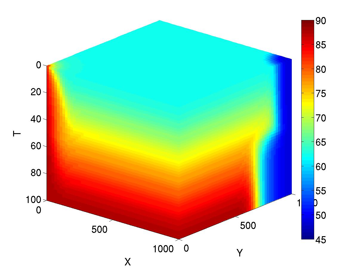
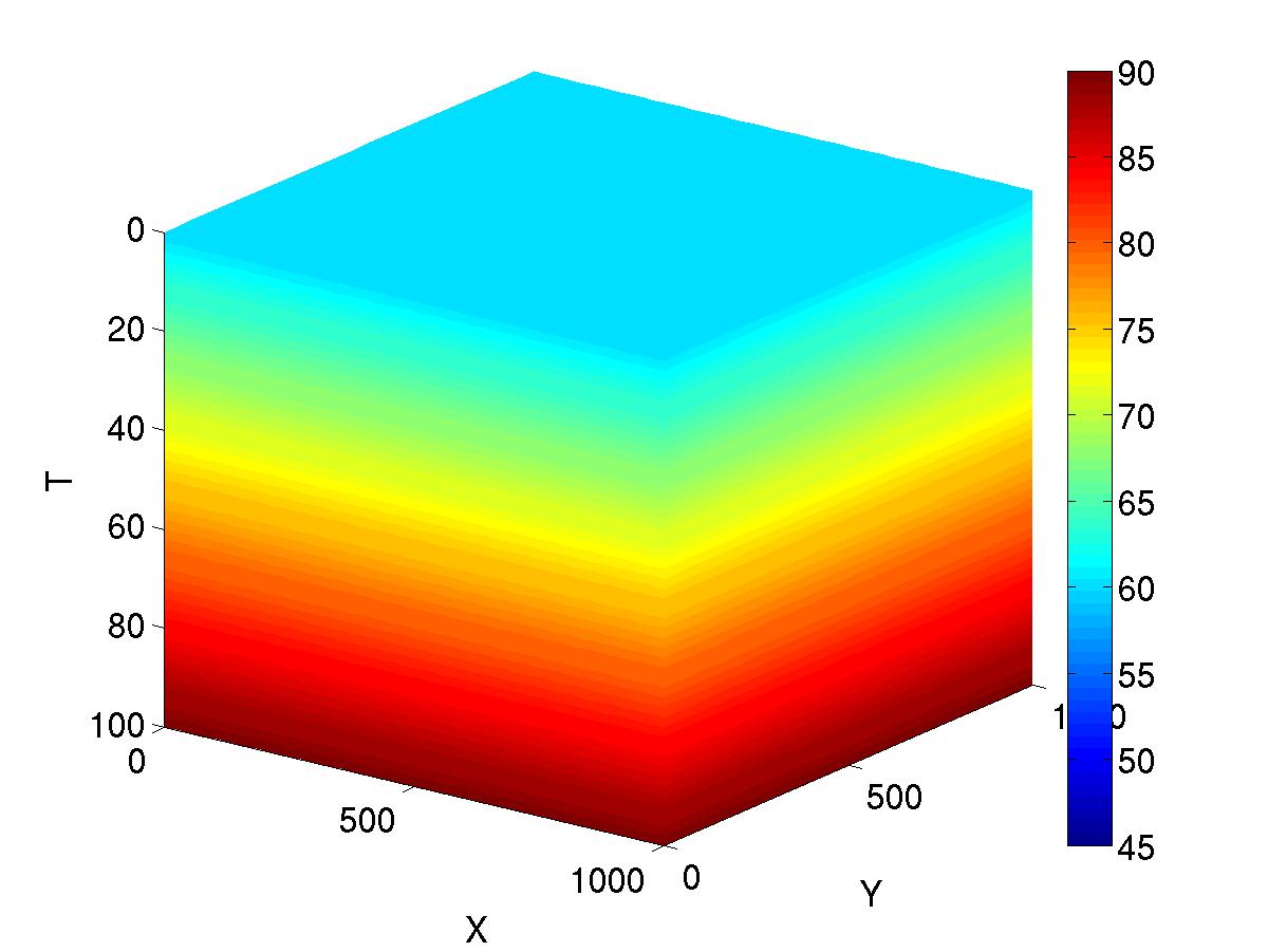
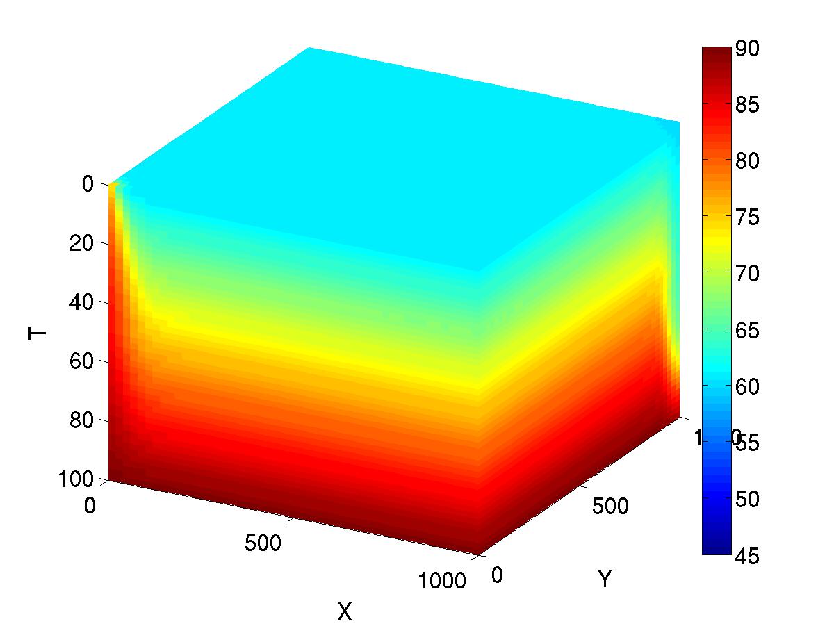
The initial temperature field is presented in Figure 1, the temperature field at $\tau=40$ days is shown in Figure 1 while Figure 1 shows the temperature at $\tau=1000$ days. We can observe that the cold water decreases reservoir temperature at injection well and that the temperature at the production well increases.

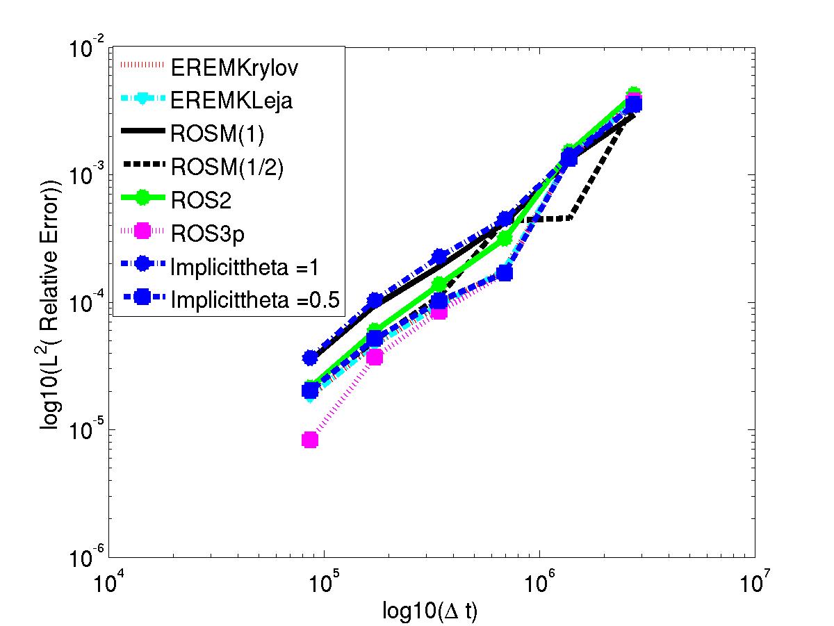
Figure 1 shows how the temperature errors at the final time $\tau=40$ days decrease with time step size. From this figure we can observe that the schemes with the same order of convergence in time have almost the same errors with our sequential approach. We can also observe that for large time steps, the errors are almost the same for all the schemes. The implicit $\theta$-Euler method with $\theta=1$ and the ROSM(1) are both of order $1.25$ in time. This order may decrease up to 1 for less smooth solutions [31] or relatively small time steps as for simple problems these schemes are order 1. We can observe that the EREM scheme and the implicit $\theta$-Euler method with $\theta=1/2$ are slightly more accurate than the ROS2 scheme. EREM scheme and the implicit $\theta$-Euler method with $\theta=1/2$ are $1.55$ in time, the ROS2(1) scheme is order $1.52$ and the ROS3p scheme is order $1.75$. This order may decrease for less smooth solutions [31]. We can however observe that schemes with high orders in time for simple problems are affected by order reduction in the sequential approach.

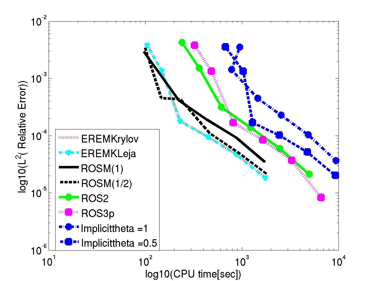
Figure 1 shows the relative $L^{2}$ temperature errors as the function of the CPU time corresponding to Figure 1. We can observe the efficiency of the EREM scheme comparing the others schemes. This figure also shows that the Exponential Rosenbrock-Euler Method and Rosenbrock- Type methods are very efficient as compared to the standard implicit $\theta$-Euler methods.

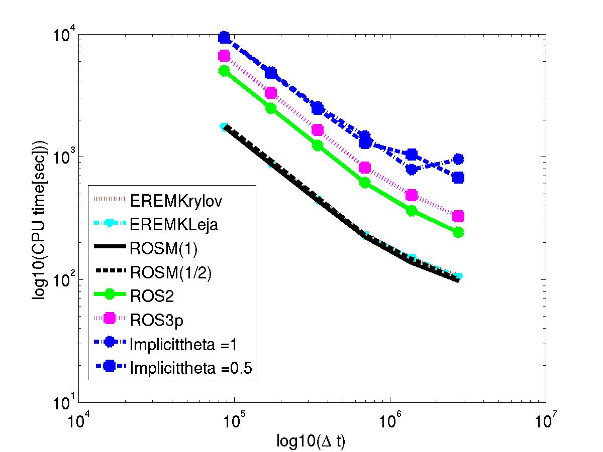
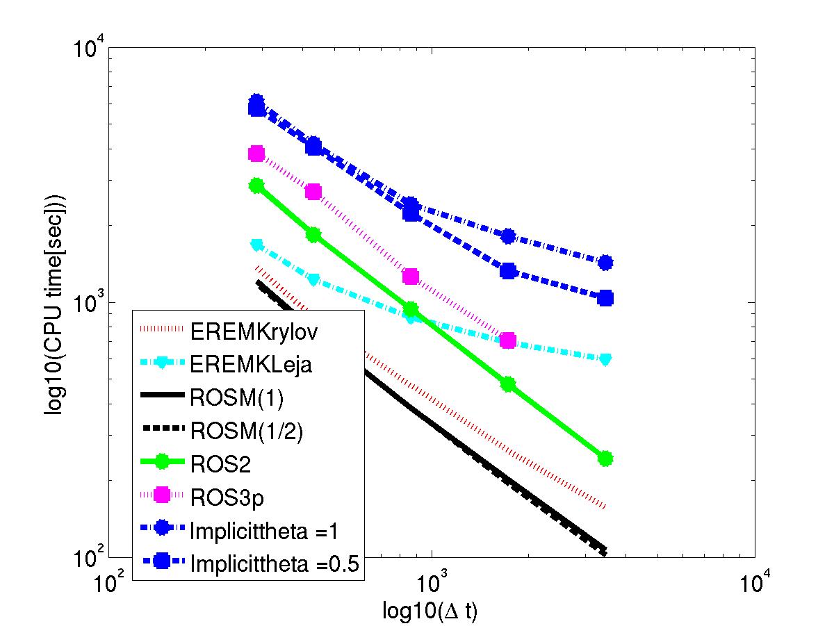
Figure 1 shows the CPU time as a function of time step size corresponding to Figure 1 and Figure 1. We can clearly observe that the Exponential Rosenbrock-Euler Method and Rosenbrock- Type methods are again very efficiency compared to standard implicit $\theta$-Euler methods. From this figure we can observe that EREM scheme, ROSM(1) and ROSM(1/2) schemes are at least five time as efficient, the ROS2 is at least twice as efficient and the ROS3p at least one and half time as efficient as the standard methods. While these factors may be dependent on the particular implementation, and the availability of good nonlinear solvers for the nonlinear solves in the standard methods, we believe them to be representative.

Figure 1: (a) Initial temperature field, (b) temperature field at $\tau=40$ days, (c) temperature field at $\tau=1000$ days, (d) the $L^{2}$ errors of the temperature as a function of time step size at the final time $\tau=40$ days, (e) the corresponding $L^{2}$ errors as a function of CPU time, and (f) CPU time as a function of time step size.

5.2 2D Fractured Geothermal Reservoir Simulation

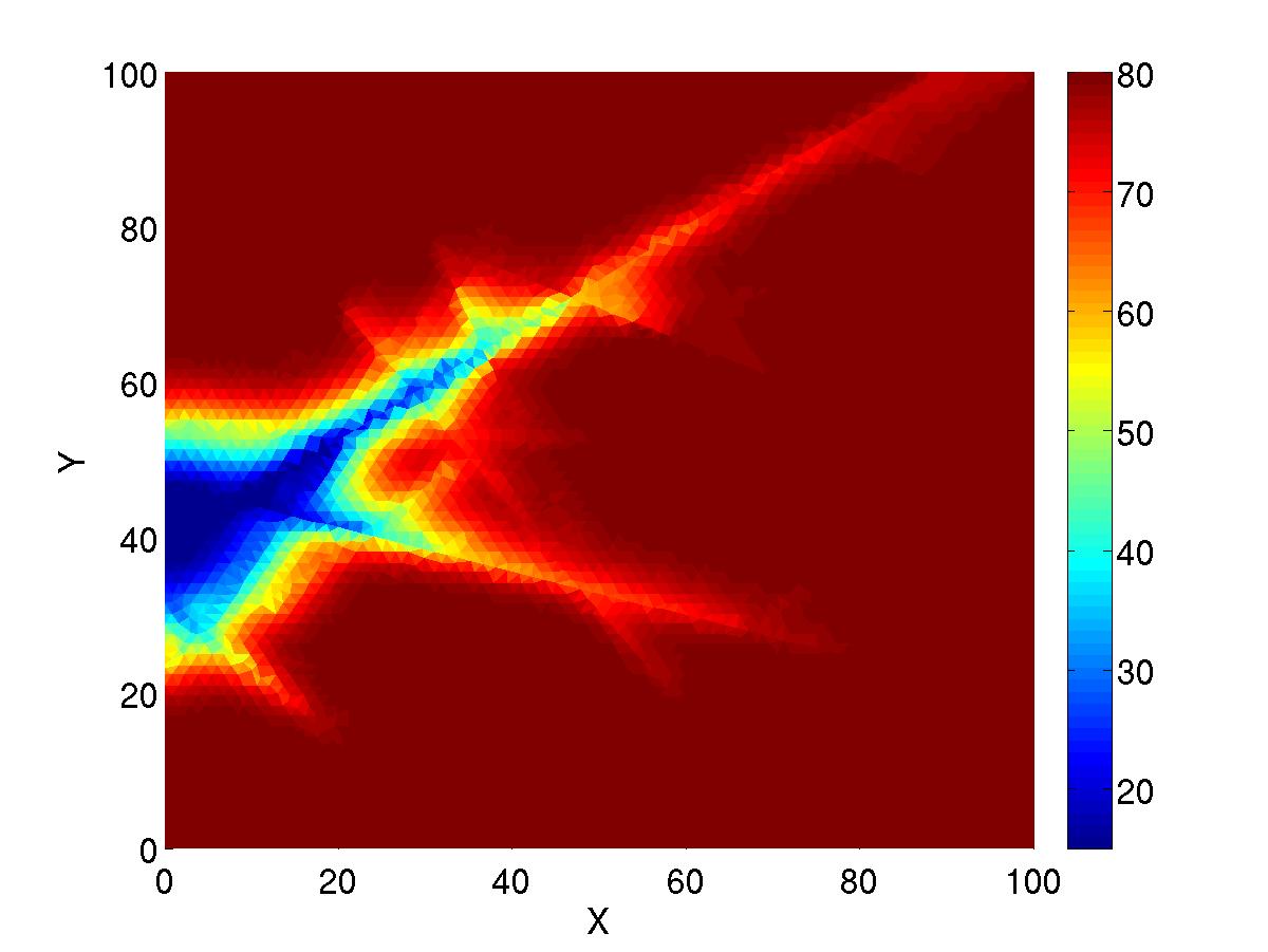
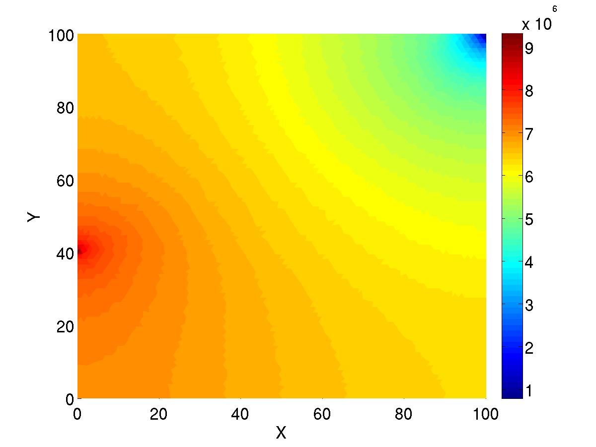
We consider here a 2 D fractured reservoir [39, 26], with a quasi-structured triangular mesh in the domain $\Omega=\left[0,100\right]\times\left[0,100\right]$, where all distances are in m. The matrix properties are: permeability $10^{-2}$ Darcy, porosity $\phi=20\%$,  $c_{ps}=1000\,J/(Kg.K)$, $\rho_{s}=2800\,kg/m^{3}$, $k_{s}=2W/(m.K)$ and $\alpha_{b}=0$. The fractures have an aperture of $10^{-3}m$ and a permeability of $100$ Darcy. The injection point is located at the position $(0,40)$, with constant pressure $10$MPa, while the production point is located at the point $(100,100)$, with constant pressure $10^{5}$Pa.

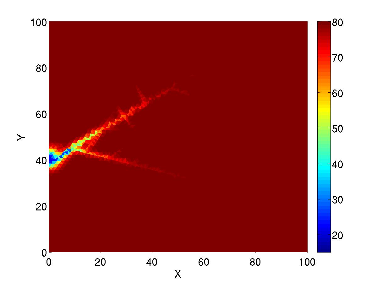
Homogeneous Neumann boundary conditions are applied for both the pressure equation given by the mass conservation law and the energy equation. The size of the system is $11460\times 11460$ for the ODEs (45) and $22920\times 22920$ for the ODEs (41). The initial temperature is $80^{o}\,\text{C}$ while the water temperature at the injection well is $15^{o}\,\text{C}$.

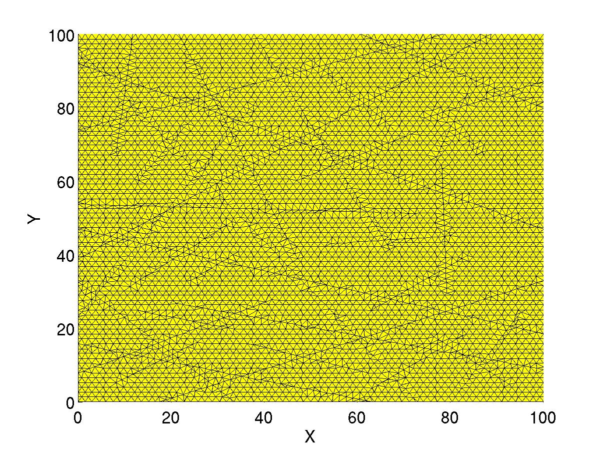
The 2D grid with fractures is shown in Figure 2, the temperature field at time $\tau=10$ days in Figure 2 and the temperature field at the time $\tau=100$ days in Figure 2. Figure 2 shows the pressure field at time $\tau=10$ days.

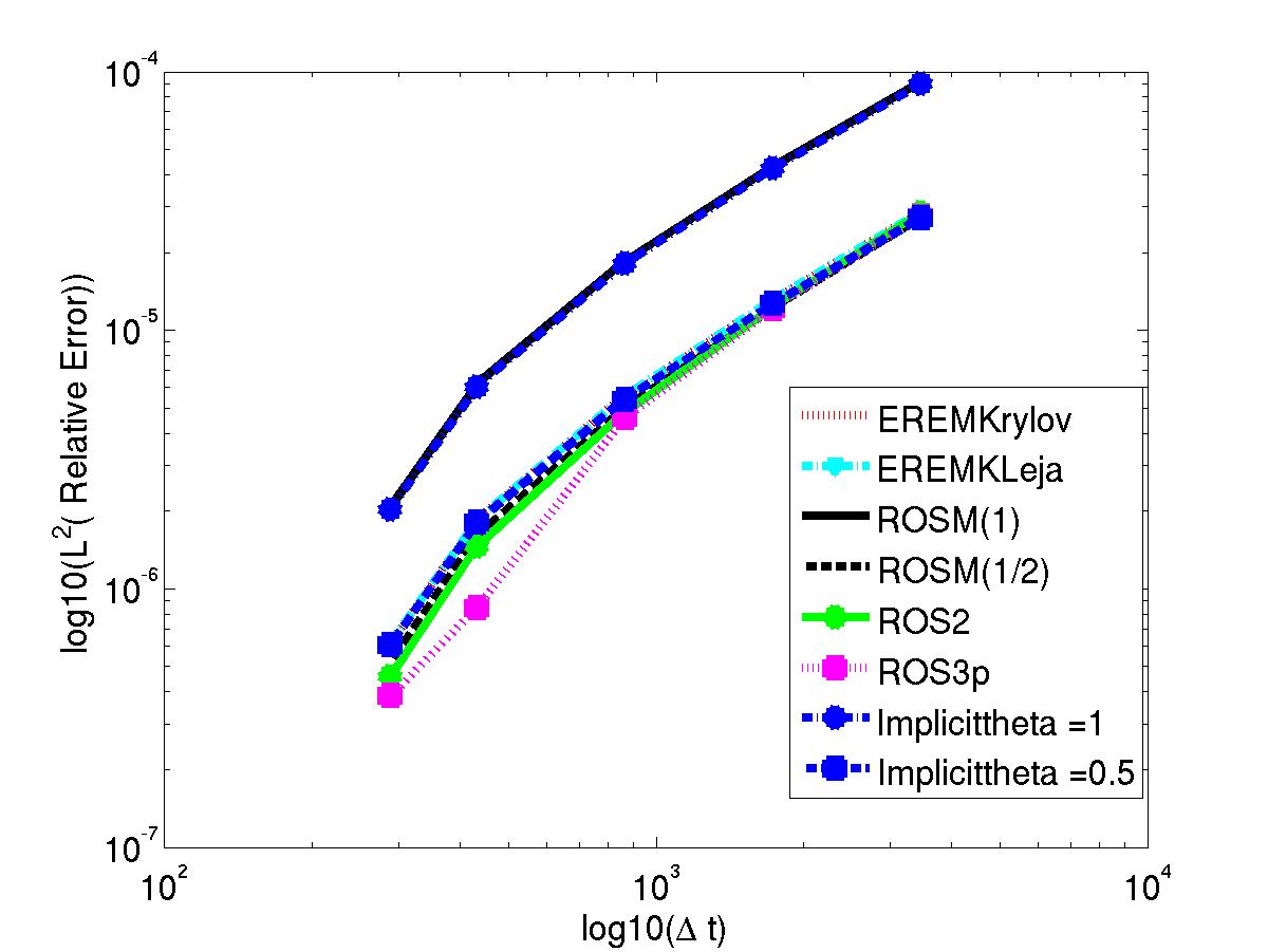
Figure 3 shows the time convergence of the all the schemes as the temperature errors decrease with time step size at the final time $\tau=10$ days. From this figure we can observe again that the schemes with the same order of convergence in time have almost the same errors. The implicit $\theta$-Euler method with $\theta=1$ and the ROSM(1) are order $1.4$ in time. The EREM scheme, the $\theta$-Euler method with $\theta=1/2$ and the ROS2(1) scheme are order $1.50$ in time while the ROS3p scheme is order $1.75$. These orders may increase for relatively small time steps. Again we can observe that schemes with high orders in time for simple problems are affected by order reduction in the sequential approach.

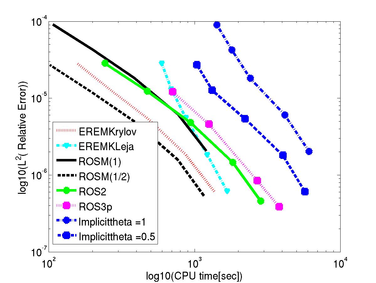
Figure 3 shows the relative $L^{2}$ temperature errors as function of the CPU time corresponding to Figure 3. As in the first example, we can observe the efficiency of the schemes ROSM(1/2) and EREM with the Krylov technique compared to the others schemes.

Figure 3 shows the CPU time as a function of time step size, corresponding to figure Figure 3 and Figure 3. Again we observe that EREM scheme, ROSM(1) and ROSM(1/2) schemes are almost four times as efficient as the standard implicit methods, while the ROS2 and the ROS3p are almost twice as efficient as the standard implicit methods. From these examples, we expect the efficiency gain to increase with the size of the problem.

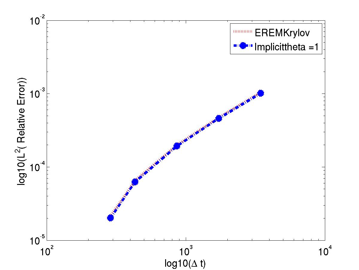
The relative $L^{2}$ pressure errors are almost the same for all the numerical schemes. We therefore plot only the errors for two numerical schemes with order 1 and 2 in time respectively. Figure 3 shows the pressure errors at time $\tau=10$ days as a function of time step size for the EREM scheme and $\theta$-Euler method with $\theta=1$. We can observe the convergence of those schemes while solving the pressure equation. The order of convergence in time is $1.5$ and may decrease according to [31] for rough solutions (less smooth solutions).

6 Conclusion

We have proposed a novel approach for simulation of geothermal processes in heterogeneous porous media. This approach decouples the mass conservation equation from the energy equation and solves each stiff ODEs from space discretization sequentially using the Exponential Rosenbrock-Euler method and Rosenbrock-type methods for the time integration.

Numerical simulations in 2D and 3D show that using the Krylov subspace technique and Real Leja points technique in the computation of the exponential functions $\varphi_{i}$ in the Exponential Rosenbrock-Euler method, and the Matlab function bicgstab with ILU(0) preconditioners with no fill-in for solving all linear systems appearing in the Rosenbrock-type methods and the implicit Euler theta methods, makes our approach more efficient compared to the sequential standard implicit Euler methods.

References

• [1] I. Aavatsmark. An introduction to multipoint flux approximations for quadrilateral grids. Comput. Geosci.,6(3-4):405–432, 2002.
• [2] S.  S.  Artemiev and T . A.  Averina. Numerical analysis of systems of ordinary and stochastic differential equations . VSP, Utrecht, Netherlands, 1997.
• [3] L. Bergamaschi, M. Caliari and M. Vianello. The RELPM exponential integrator for FE discretizations of advection-diffusion equations, in: M. Bubak, G. D.  Van Albada, P. Sloot (Eds.), Lecture Notes in Computer Sciences Volume 3039, Springer Verlag, Berlin Heidelberg, 2004, pp. 434-442.
• [4] J. Bundschuh and M.C. Suárez Arriaga. Introduction to the Numerical Modeling of Groundwater and Geothermal Systems CRC Press, 2010.
• [5] M. Caliari, and A. Ostermann. Implementation of exponential Rosenbrock-type integrators. Applied Numerical Mathematics, 568-581 (59),2009.
• [6] M. Caliari, A. Ostermann and S.  Rainer. Meshfree exponential Integrators. Submitted, 2010.
• [7] M. Caliari, M. Vianello and L. Bergamaschi. Interpolating discrete advection diffusion propagators at Léja sequences. Journal of Computational and Applied Mathematics, 172(1):79–99, 2004.
• [8] E.  J.  Carr, T.  J.  Moroney and I. W.  Turner. Efficient simulation of unsaturated flow using exponential time integration. Applied Mathematics and Computation, 217(14): 6587–6596, 2011.
• [9] Z. Chen, G. Huan and Y .Ma. Computational Methods for Multiphase Flows in Porous Media SIAM, 2006.
• [10] K. Císařová, J. Kopal,J. Královcová and J. Maryška. Simulation of geothermal processes. Proceedings World Geothermal Congress, Bali, Indonesia, 2010.
• [11] D.  Coumou, T. Driesner, S.  Geiger, C. A.  Heinrich and S.  K.  Matthäi. The dynamics of mid-ocean ridge hydrothermal systems: Splitting plumes and fluctuating vent temperatures. Earth and Planetary Science Letters, 245, pp. 218–231, 2006.
• [12] S. M. Cox and P. C. Matthews. Exponential time differencing for stiff systems. Journal of Computational Physics, 176(2):430–455, 2002.
• [13] R. Eymard, T. Gallouet and R. Herbin. Finite volume methods, in: P. G. Ciarlet, J. L. Lions (Eds.), Handbook of Numerical Analysis Volume 7, North-Holland, Amsterdam, 2000, pp. 713–1020.
• [14] R. Eymard, and T. Gallouet and R. Herbin. A cell-centred finite-volume approximation for anisotropic diffusion operators on unstructured meshes in any space dimension. IMA Journal of Numerical Analysis, 26:326–353, 2006.
• [15] R.  A.  Fine and F. J. Millero. Compressibility of water as a function of temperature and pressure. J. Chem. Phys, 59, 5529,1973.
• [16] S. Geiger, T.  Driesner, C.  A..  Heinrich and S.  K.  Matthäi. Multiphase Thermohaline Convection in the EarthCrust: I. A New Finite Element – Finite Volume Solution Technique Combined With a New Equation of State for NaCl-H2O. Transport in Porous Media, (63):399–434, 2006.
• [17] G.  Geiger, G. J.Lord and A.  Tambue. Exponential time integrators for stochastic partial differential equations in 3D reservoir simulation. Computational Geosciences, 16(2), pp. 323–334, 2012.
• [18] T.  Graf. Simulation of Geothermal Flow in Deep Sedimentary Basins in Alberta. Alberta Geological Survey, 2009.
• [19] L.  Haar, J.  Gallagher and G.  Kell. NBS/NRC Steam Tables. Academic Press., 1982.
• [20] E.  Hairer and G.  Wanner. Solving Ordinary Differential Equations II: Stiff and Differential- Algebraic Problems. Second Revised Editions, Springer series In Lecture Notes in Computational Mathematics 14, Springer-Verlag Berlin Heidelberg, 1996.
• [21] D. O. Hayba and S. Ingebritsen. The computer model HYDROTHERM, a three-dimensional finite–difference model to simulate ground–water flow and heat transport in the temperature range of 0 to 12000Csuperscript12000𝐶1200^{0}C. Geol. Surv. Water Res. Invest. Report. 94–12252, 1994.
• [22] M. Hochbruck and C. Lubich, On Krylov subspace approximations to the matrix exponential operator, SIAM J. Numer. Anal. 34(5):1911–1925, 1997.
• [23] M.  Hochbruck and A.  Ostermann. Exponential integrators. Acta Numerica, 209–286, doi:10.1017/S0962492910000048, 2010.
• [24] M.  Hochbruck, A.  Ostermann and J.  Schweitzer. Exponential Rosenbrock-Type Methods. SIAM J. NUMER. ANAL., 47(1):786–803, 2009.
• [25] S.  E. Ingebritsen, S. Geiger, S.  Hurwitz and T.  Driesner. Numerical simulation of magmatic hydrothermal. Rev. Geophys., 48, RG1002, doi:10.1029/2009RG000287, 2010.
• [26] M. Karimi-Fard, L. Durlofsky and K. Aziz. An efficient discrete-fracture model applicable for general-purpose reservoir simulators. SPE J 9, pp. 227–236, 2004.
• [27] D. A. Knoll and D. E. Keyes. Jacobian-free Newton-Krylov methods: A survey of approaches and application Journal of Computational Physics, 193 (2): 357–397, 2004.
• [28] J. Lang. Adaptive Multilevel Solution of Nonlinear Parabolic PDE Systems. Theory, Algorithm and Applications. Lecture Notes in Computational Science and Engineering, Springer Berlin , 2001.
• [29] J. Lang and J. Verwer. ROS3P– An Accurate Third -order Rosenbrock Solver Designed for Parabolic Problems. BIT Numerical Mathematics, 41(4):731–738, 2001.
• [30] K.-A. Lie, S.  Krogstad, I.  S. Ligaarden, J. R.  Natvig, H. M. Nilsen and B.  Skaflestad. Open Source MATLAB Implementation of Consistent Discretisations on Complex Grids. Comput.Geosci., 16(2):297-322, 2012.
• [31] H. Holden, K.  H. Karlsen,K.-A. Lie and N. H. Risebro. Splitting Methods for Partial Differential Equations with Rough Solutions: Analysis and MATLAB programs. European Mathematical Society Publishing House, Zürich, Switzerland, 2010.
• [32] A. Martínez, L.  Bergamaschi, M. Caliari and M. Vianello. A massively parallel exponential integrator for advection-diffusion models. Journal of Computational and Applied Mathematics 231, 82–91, 2009.
• [33] C. Moler and C. Van Loan. Ninteen Dubious Ways to Compute the Exponential of a Matrix, Twenty–Five Years Later, SIAM Review 45(1): 3–49, 2003.
• [34] D.  A. Nield and A.  Bejan. Convection in Porous Media. Third Edition. New York: Springer Science+Business Media, Inc., 2006.
• [35] J. Niesen, and W. Wright. Algorithm 919: A Krylov subspace algorithm for evaluating the φlimit-from𝜑\varphi-functions appearing in exponential integrators. ACM Trans. Math. Softw., 38(3), Article 22, 2012.
• [36] R. Podgorney, H. Huang and D. Gaston. Massively parallel fully coupled implicit modeling of coupled thermal-hydrological-mechanical processes for enhanced geothermal system reservoirs, Proceedings, Thirty-Fifth Workshop on Geothermal Reservoir Engineering Stanford University, Stanford, California, 2010, SGP-TR-188.
• [37] K. Pruess, TOUGH2: A general-purpose numerical simulator for multiphase fluid and heat flow, Report LBL-29400, Lawrence Berkeley Laboratory, Berkeley, CA, May 1991.
• [38] L. Reichel. Newton interpolation at Léja points. BIT Numerical Mathematics 30(2):332–346, 1990.
• [39] T.  H.  Sandve, I. Berre and J.  M. Nordbotten. An efficient Multi-Point Flux Approximation method for Discrete Fracture-Matrix simulations. Journal of Computational Physics, 231(9), 3784–3800, 2012.
• [40] R. B. Sidje. Expokit: A software package for computing matrix exponentials, ACM Trans. Math. Software 24(1):130–156, 1998.
• [41] A.Tambue. Efficient Numerical Methods for Porous Media Flow. PhD Thesis, Department of Mathematics, Heriot–Watt University, 2010.
• [42] A. Tambue. Space & time errors estimates for the combined Finite Volume–Exponential integrator for nonlinear reactive flow. Submitted, 2011.
• [43] A.  Tambue, I. Berre, J.  M. Nordbotten and T.  H.  Sandve. Exponential Euler time Integrator for simulation of geothermal Processes in Heterogeneous porous Media. Proceedings, Thirty-Seventh Workshop on Geothermal Reservoir Engineering Stanford University, Stanford, California, 2012, SGP-TR-194.
• [44] A. Tambue, and S. Geiger and G. J.  Lord. Exponential Time integrators for 3D Reservoir Simulation. In proceedings of the 12th European Conference on the Mathematics of Oil Recovery, Oxford, UK, 2010.
• [45] A.  Tambue, G. J.Lord and S.  Geiger. An exponential integrator for advection-dominated reactive transport in heterogeneous porous media. Journal of Computational Physics , 229(10):3957–3969, 2010.
• [46] J. W. Thomas, Numerical partial differential equations: finite difference methods, Springer Verlag, Berlin Heidelberg New York, 1995.