Interpretations and Implications of the Top Quark
Rapidity Asymmetries $A_{FB}^{t}$ and $A_{FB}^{\ell}$

Abstract

Forward-backward asymmetries $A_{FB}^{t}$ and $A_{FB}^{\ell}$ are observed in the top quark $t$ rapidity distribution and in the rapidity distribution of charged leptons $\ell$ from top quark decay at the Tevatron proton-antiproton collider, and a charge asymmetry $A_{C}$ is seen in proton-proton collisions at the Large Hadron Collider (LHC). In this paper, we update our previous studies of the Tevatron asymmetries using the most recent data. We provide expectations for $A_{C}$ at the LHC based first on simple extrapolations from the Tevatron, and second based on new physics models that can explain the Tevatron asymmetries. We examine the relationship of the two asymmetries $A_{FB}^{t}$ and $A_{FB}^{\ell}$. We show their connection through the $(V-A)$ spin correlation between the charged lepton and the top quark with different polarization states. We show that the ratio of the two asymmetries provides independent insight into the physics interpretation of the top quark asymmetry. We emphasize the value of the measurement of both asymmetries, and we conclude that a model which produces more right-handed than left-handed top quarks is suggested by the present Tevatron data.

I Introduction

The observation of a larger than expected forward-backward asymmetry $A_{FB}^{t}$ in the rapidity of top quarks produced at the Fermilab Tevatron collider Aaltonen et al. (2011); Abazov et al. (2011) continues to hold considerable attention in the community of particle physicists. It is one of few manifestations of a deviation from predictions of the standard model (SM). That the deviation occurs in the top sector suggests that its interpretation might well involve new physics (NP), given that the large mass of the top quark is comparable in value to the electroweak scale. Indeed, many NP models have been proposed to explain the enhancement of $A_{FB}^{t}$. These models usually postulate the existence of new states, whether in the direct-channel coupling to $t\bar{t}$, or exchanged in a cross-channel and coupling the top quark to first- and/or second-generation quarks. Examples include flavor-changing $Z^{\prime}$ Jung et al. (2010); Cao et al. (2010a); Xiao et al. (2010a); Cao et al. (2011); Berger et al. (2011); Zhou et al. (2011); Aguilar-Saavedra and Perez-Victoria (2011a); Gresham et al. (2011); Aguilar-Saavedra and Perez-Victoria (2011b, c); Duraisamy et al. (2011); Aguilar-Saavedra and Perez-Victoria (2011c); Gresham et al. (2012a); Ko et al. (2012a, b, c, d); Li et al. (2012); Ko et al. (2012e); Alvarez and Leskow (2012); Drobnak et al. (2012a); Aguilar-Saavedra and Perez-Victoria (2011c), $W^{\prime}$ Cheung et al. (2009); Barger et al. (2010); Cheung and Yuan (2011); Barger et al. (2011); Bhattacherjee et al. (2011); Craig et al. (2011); Chen et al. (2011a); Cao et al. (2012); Yan et al. (2012); Knapen et al. (2012); Duffty et al. (2012); Adelman et al. (2012); Endo and Iwamoto (2012) and axigluon $G^{\prime}$ Antunano et al. (2008); Ferrario and Rodrigo (2008); Ferrario and Rodrigo (2009a, b); Frampton et al. (2010); Cao et al. (2010b); Chivukula et al. (2010); Xiao et al. (2010b); Bai et al. (2011); Wang et al. (2011a); Marques Tavares and Schmaltz (2011); Alvarez et al. (2011a); Aguilar-Saavedra and Perez-Victoria (2011d); Wang et al. (2011b); Krnjaic (2012); Aguilar-Saavedra and Santiago (2012); Gabrielli et al. (2012); Zhu et al. (2012); Cvetic et al. (2012); Dutta et al. (2012); Gross et al. (2012); Gresham et al. (2012b) models, among others  Djouadi et al. (2010); Shu et al. (2010); Arhrib et al. (2010); Dorsner et al. (2010); Bauer et al. (2010); Chen et al. (2011b); Alvarez et al. (2011b); Patel and Sharma (2011); Zerwekh (2011); Barreto et al. (2011); Foot (2011); Jung et al. (2011a, b); Babu et al. (2011); Djouadi et al. (2011); Hektor et al. (2011); Cui et al. (2011); Frank et al. (2011); Davoudiasl et al. (2012); Jung et al. (2011c); Kosnik et al. (2011); de la Puente (2012); Wang et al. (2012); Endo and Iwamoto (2012); Drobnak et al. (2012b).

Strong constraints on models of new physics come from a variety of sources, whether from low-energy precision data that limit flavor changing couplings of the top quark, or from collider data such as the $t\bar{t}$ invariant mass distribution and the $t\bar{t}$ total cross section at the Tevatron. Models of NP also face experimental constraints from searches for new phenomena at the LHC such as the absence of direct evidence thus far for new heavy gauge bosons $W^{\prime}$  Chatrchyan et al. (2012a) and $Z^{\prime}$, and strong bounds on the cross section at the LHC for the production of pairs of same-sign top quarks Aad et al. (2012a); Chatrchyan et al. (2012b).

Of particular interest to us have been the implications of models of new physics for the polarization of the top quark, and methods that can be used to measure the polarization Berger et al. (2012a). This focus on the top quark polarization also serves as a unifying theme for the topics discussed in this new paper. In the SM, strong production of $t\bar{t}$ pairs in quantum chromodynamics (QCD) yields an equal number of positive and negative helicity top quarks, hereafter referred to as $t_{R}$ and $t_{L}$. Electroweak production in single top quark production, for example, yields primarily $t_{L}$. Therefore, a demonstration that a significant fraction of top quarks are produced with positive helicity would herald new physics.

In addition to $A_{FB}^{t}$ of the top quark, the D0 group reports a positive forward-backward asymmetry of charged leptons from top quark decays. The measurement is done in two ways Abazov et al. (2011, 2012), both based on data corresponding to an integrated luminosity of $5.4\rm{~{}fb}^{-1}$. The value $A_{FB}^{\ell}=(15.2\pm 4.0)\%$ is measured in the $\ell$+jets final states Abazov et al. (2011). The second method uses the dilepton final states from $t\bar{t}$ production, where the $W$ bosons from the $t$ and $\bar{t}$ decays both decay leptonically. The result obtained is $A^{\ell}_{\rm FB}=(5.8\pm 5.1({\rm stat})\pm 1.3({\rm syst}))$%. A combination of the two measurements yields $A^{\ell}_{\rm FB}={11.8\pm 3.2}\%$. The combined result may be compared with the values $(2.1\pm 0.1)\%$ from simulations of the SM or $(4.7\pm 0.1)\%$ once QCD+EW corrections are included Bernreuther and Si (2010); Abazov et al. (2012), an excess at the level of 2.2 standard deviations. In a previous paper, we investigated the kinematic and dynamic relationship between the two asymmetries $A_{FB}^{t}$ and $A_{FB}^{\ell}$ Berger et al. (2012b). The fact that $A_{FB}^{\ell}$ and $A_{FB}^{t}$ are larger than the SM predictions indicates that the charged lepton strongly prefers to move in the same direction as the top quark from which it originates Krohn et al. (2011); Falkowski et al. (2011). Data on the ratio of the two asymmetries tend to favor models in which more $t_{R}$ than $t_{L}$ are produced, but confirmation with greater statistical and systematic precision is desirable. A detailed analysis of the SM prediction of the lepton charge asymmetry at the Tevatron and the LHC can be found in Ref. Bernreuther and Si (2012).

In this paper, we elaborate on the studies reported earlier and include new predictions. We begin in Sec. II with the definitions of the asymmetries measured at the Tevatron. We summarize the Tevatron data and, using the latest data, we update our earlier fits in the framework of $Z^{\prime}$, $W^{\prime}$, and axigluon new physics models. Unlike the Tevatron proton-antiproton collider, the LHC proton-proton collider offers no preferred direction for the measurement a rapidity asymmetry. Nevertheless, a charge asymmetries $A_{C}^{t}$ for top quarks and $A_{C}^{\ell}$ for leptons can be defined and predicted in the SM. Using data from the Tevatron, we estimate what may be observed for these charge asymmetries at the LHC in the context of models of new physics, and we compare these expectations with LHC data in in Sec. III. As we show, despite limited statistics, the LHC data on the charge asymmetry are also consistent with a deviation from the SM, although perhaps not as great a deviation as expected from an extrapolation from the Tevatron observations.

The relationship of $A_{FB}^{t}$ and $A_{FB}^{\ell}$ is addressed in Sec. IV and in Appendix A where we include detailed derivations of results not published before. The essential starting point is the $V-A$ structure of the matrix element for the decay $t\rightarrow W^{+}b\rightarrow b\ell^{+}\nu$. Section IV.1 contains a discussion of the angular distribution of decay lepton $\ell^{+}$, first in the rest frame of the top quark and then after the top quark is boosted in rapidity and transverse momentum. We pay particular attention to the positive/negative helicity state of the top quark because the final momentum and angular distributions of leptons in the laboratory frame, after the top quark is boosted, depends significantly on the top quark’s polarization state. In Sec. IV, we derive the relationship of the lepton asymmetry $A_{FB}^{\ell}$ and the top quark asymmetry $A_{FB}^{t}$ separately for the left- and right-handed polarization states of the top quark.

Different models of new physics produce top quarks with different proportions of left- and right-handed polarization. For example, $Z^{\prime}$ and $W^{\prime}$ models produce predominantly right-handed top quarks, whereas the axigluon model generates unpolarized top quarks. We use an axigluon model and a $W^{\prime}$ model in Sec. V to deduce their different expectations for the ratio of the lepton and top quark asymmetries. In the case of both models, the allowed parameters produce a range of values for the ratios $A_{C}^{\ell}/A_{C}^{t}$ at the LHC and $A_{FB}^{\ell}/A_{FB}^{t}$ at the Tevatron, aligned along approximately straight lines in plots of $A_{C}^{\ell}$ vs $A_{C}^{t}$ and of $A_{FB}^{\ell}$ vs $A_{FB}^{t}$. Ideally, precise data would provide a definite point in the two dimensional plot and tightly constrain the parameter space.

Our conclusions appear in Sec. VI. We emphasize the value of making measurements both of $A_{FB}^{t}$ and $A_{FB}^{\ell}$ and of $A_{C}^{\ell}$ and $A_{C}^{t}$ because their ratio can be related through top quark polarization to the underlying dynamics of top quark production.

II Tevatron Data and Updated Fits

The top quark forward-backward asymmetry in $t\bar{t}$ pair production at the Tevatron is defined as

$$A_{FB}^{t}=\frac{N(\Delta y>0)-N(\Delta y<0)}{N(\Delta y>0)+N(\Delta y<0)},$$ (1)

where $\Delta y=y_{t}-y_{\bar{t}}$ is the difference between the rapidities of the top quark and the anti-top quark, and $N(\Delta y>0)$ ($N(\Delta y<0)$) is the number of events with $\Delta y>0$ ($\Delta y<0$). The proton beam is chosen as the direction of positive $z$. In the SM, the asymmetry is induced by perturbative diagrams beyond the leading order. It is predicted to be $(8.7\pm 1.0)\%$, including NLO EW and QCD corrections Kuhn and Rodrigo (1998, 2012). The most recent D0 result in the $t\bar{t}$ rest frame is $A_{FB}^{t}=(19.6\pm 6.5)\%$  Abazov et al. (2011), based on their $5.4~{}\rm{fb}^{-1}$ luminosity data set, while the measurement from CDF is $(16.2\pm 4.7)\%$ based on their data set with integrated luminosity of $8.7~{}\rm{fb}^{-1}$ Aaltonen et al. (2012). CDF also reports that $A_{FB}^{t}$ in the region of large $t\bar{t}$ pair invariant mass ($m_{t\bar{t}}\geq 450~{}\rm{GeV}$) exceeds the SM prediction ($\sim 3\sigma$), although the significance is not as large as the $3.4\sigma$ deviation of CDF’s previous result Aaltonen et al. (2011). More explicitly, $A_{FB}^{t}(m_{t\bar{t}}\geq 450~{}\rm{GeV})=(29.6\pm 6.7)\%$ and the SM prediction is $(12.8\pm 1.1)\%$ Kuhn and Rodrigo (2012).

Many new physics models have been proposed to explain the discrepancy of $A_{FB}^{t}$ between data and the SM prediction. Some of these models are now quite sophisticated. It is not our intention in this paper to investigate models in detail. Rather, we explore a few simple models as illustrations of a range of possibilities. We begin in this section with an update of our previous fits to Tevatron data for three models: flavor-changing $Z^{\prime}$ exchange, flavor-changing $W^{\prime}$ exchange, and axigluon models. The minimal version of the $Z^{\prime}$ model implies a large rate for same-sign top quark pair production at the LHC, not supported by data Berger et al. (2011); Aad et al. (2012a); Chatrchyan et al. (2012b). The $W^{\prime}$ model is highly constrained by data on the $t\bar{t}$ plus jets final state at the LHC Knapen et al. (2012); Duffty et al. (2012); Chatrchyan et al. (2012a).

The effective interaction between a flavor-changing $Z^{\prime}$/$W^{\prime}$ and SM particles is

$$\mathcal{L}=\frac{g_{2}f_{V^{\prime}}}{\sqrt{2}}\bar{q}\gamma^{\mu}P_{R}tV^{\prime}_{\mu}+h.c.~{},$$ (2)

where $g_{2}$ is the weak coupling, and $q=u~{}(d)$ for $V^{\prime}=Z^{\prime}(W^{\prime})$. In addition to the SM process $q\bar{q}\to g\to t\bar{t}$ and its NLO corrections, the $t\bar{t}$ pair will also be produced via a $t$-channel process with a $Z^{\prime}$ or $W^{\prime}$ mediator. Using “$\lambda_{i}=+$” to represent the positive helicity of particle $i$ (right-handed polarization for massless particle), and “$\lambda_{i}=-$” the negative helicity (left-handed polarization for massless particle), we express the helicity amplitude $M_{V^{\prime}}^{t}(\lambda_{q},\lambda_{\bar{q}},\lambda_{t},\lambda_{\bar{t}})$, apart from a common factor $\displaystyle{\frac{g_{2}^{2}f_{V^{\prime}}^{2}\hat{s}\delta_{ac}\delta_{bd}}{8\left(\hat{t}-m_{V^{\prime}}^{2}\right)}}$, where $a,~{}b,~{}c$ and $d$ are the color indexes of $q,~{}\bar{q},~{}t$ and $\bar{t}$, as

$$\mathcal{M}_{V^{\prime}}^{t}(+---) = \left(2+r_{V}^{2}\right)\sqrt{1-\beta^{2}}\sin\theta,$$

$$\mathcal{M}_{V^{\prime}}^{t}(+--+) = \left[2(1-\beta)+r_{V}^{2}(1+\beta)\right](1-\cos\theta),$$

$$\mathcal{M}_{V^{\prime}}^{t}(+-+-) = -\left[2(1+\beta)+r_{V}^{2}(1-\beta)\right](1+\cos\theta),$$

$$\mathcal{M}_{V^{\prime}}^{t}(+-++) = -\left(2+r_{V}^{2}\right)\sqrt{1-\beta^{2}}\sin\theta~{}.$$ (3)

The variables $\hat{s}$ and $\hat{t}$ are the usual Mandelstam variables, $m_{V^{\prime}}$ is the mass of $V^{\prime}$, $r_{V}=m_{t}/m_{V^{\prime}}$, $\beta=\sqrt{1-4m_{t}^{2}/\hat{s}}$, and $\theta$ is the polar angle of the top quark in the center mass (c.m. frame) of the $t\bar{t}$ pair, measured relative to the initial state quark. In the highly boosted limit of $\beta\to 1$, the nonzero helicity amplitudes are

$$\mathcal{M}_{V^{\prime}}^{t}(+--+) \sim 2r_{V}^{2}(1-\cos\theta),$$

$$\mathcal{M}_{V^{\prime}}^{t}(+-+-) \sim -4(1+\cos\theta)~{}.$$ (4)

For the axigluon ($G^{\prime}$) model, we assume, for simplicity, that the interaction of the axigluon with the SM quarks is purely pseudo-vector-like and can be written as

$$\mathcal{L}=g_{s}\left(g_{l}~{}\bar{q_{i}}\gamma^{\mu}\gamma_{5}q_{j}+g_{h}~{}\bar{Q_{i}}\gamma^{\mu}\gamma_{5}Q_{j}\right)t^{A}_{ij}G^{\prime~{}A}_{\mu},$$ (5)

where $t_{ij}^{A}$ is the generator of the color $SU(3)$ group; $q$ denotes the first two generation quarks in the SM and $Q$ the third generation quarks. The coupling $g_{s}$ is the usual strong coupling strength; $g_{l}$ and $g_{h}$ are the coupling parameters of the axigluon to the light quark ($q$, i.e. first two generations) and the heavy quark ($Q$, i.e. third generation), respectively.

The process $q\bar{q}\to G^{\prime}\to t\bar{t}$ contributes to $t\bar{t}$ production at hadron colliders. Its helicity amplitudes $M_{G^{\prime}}(\lambda_{q},\lambda_{\bar{q}},\lambda_{t},\lambda_{\bar{t}})$ are

$$\mathcal{M}_{G^{\prime}}(+-+-) = \mathcal{M}_{G^{\prime}}(-+-+)=\frac{g_{s}^{2}t^{A}_{ba}t^{A}_{cd}\hat{s}~{}(-g_{l}g_{h})}{\hat{s}-m_{G^{\prime}}^{2}+im_{G^{\prime}}\Gamma_{G^{\prime}}}\beta(1+\cos\theta),$$

$$\mathcal{M}_{G^{\prime}}(-++-) = \mathcal{M}_{G^{\prime}}(+--+)=\frac{g_{s}^{2}t^{A}_{ba}t^{A}_{cd}\hat{s}~{}(-g_{l}g_{h})}{\hat{s}-m_{G^{\prime}}^{2}+im_{G^{\prime}}\Gamma_{G^{\prime}}}\beta(1-\cos\theta).$$ (6)

where $\Gamma_{G^{\prime}}$ is the width of axigluon. For $m_{G^{\prime}}>2m_{t}$, which is the case in our study,

$$\Gamma_{G^{\prime}}=\frac{\alpha_{S}m_{G^{\prime}}}{6}\left\{4g_{l}^{2}+g_{h}^{2}\left[1+\left(1-\frac{4m_{t}^{2}}{m_{G^{\prime}}^{2}}\right)^{3/2}\right]\right\}.$$ (7)

For coupling strength $g_{l}=g_{h}=1$, the ratio $\Gamma_{G^{\prime}}/m_{G^{\prime}}\sim 0.1$.

The absence of pronounced deviations from the SM expectation in the measured $m_{t\bar{t}}$ distribution Aaltonen et al. (2011); Abazov et al. (2011) indicates that the axigluon should be heavy and/or broad. Since the term linear in $\cos\theta$ appears only in the interference term, the contribution to $A_{FB}^{t}$ in $t\bar{t}$ production from an axigluon is therefore through interference with the SM channel. Its effect becomes important in the region of large $m_{t\bar{t}}$, i.e. $\beta\sim 1$. The interference term in the overall squared amplitude is proportional to

$$\left[2g_{l}g_{h}(1+\cos\theta)^{2}-2g_{l}g_{h}(1-\cos\theta)^{2}\right]\frac{\hat{s}(\hat{s}-m_{G^{\prime}}^{2})}{(\hat{s}-m_{G^{\prime}}^{2})^{2}+m_{G^{\prime}}^{2}\Gamma_{G^{\prime}}^{2}}=\frac{4g_{l}g_{h}\hat{s}(\hat{s}-m_{G^{\prime}}^{2})\cos\theta}{(\hat{s}-m_{G^{\prime}}^{2})^{2}+m_{G^{\prime}}^{2}\Gamma_{G^{\prime}}^{2}}.$$ (8)

When an axigluon is heavy such that $\sqrt{\hat{s}}<m_{G^{\prime}}$, the product of $g_{l}g_{h}$ must be negative to obtain a positive $A_{FB}$ Ferrario and Rodrigo (2009a); Frampton et al. (2010); Cao et al. (2010b).

We fit data at the Tevatron to determine the parameters of the three new physics models under consideration. The SM contributions at NLO are included along with the contributions from the new physics models. We choose to fit the measured inclusive total cross section for $t\bar{t}$ production $7.5\pm 0.31({\text{stat}})\pm 0.34({\text{syst}})\pm 0.15({\text{Z~{}theory}})~{}{\rm pb}$ Aaltonen et al. (2009), and $A_{FB}^{t}$ from CDF with $8.7~{}\rm{fb}^{-1}$ integrated luminosity Aaltonen et al. (2012). We scan the parameter space of the models requiring that the predictions fit the total cross section as well as $A_{FB}^{t}$ for both $m_{t\bar{t}}<~{}450~{}{\rm GeV}~{}(7.8\%\pm 5.4\%)$ and $m_{t\bar{t}}\geq~{}450~{}{\rm GeV}~{}(29.6\%\pm 6.7\%)$ within $2\sigma$ accuracy. The SM $t\bar{t}$ cross section we adopt is $6.77\pm 0.73~{}\rm{pb}$ calculated with MCFM6.2 Campbell et al. (2012). For the SM predictions of $A_{FB}^{t}$ in different energy bins, we follow the values shown in Ref. Kuhn and Rodrigo (2012):

$$A_{FB}^{t}(m_{t\bar{t}}<~{}450~{}{\rm GeV})=(6.2\pm 0.4)~{}\%,~{}~{}A_{FB}^{t}(m_{t\bar{t}}\geq~{}450~{}{\rm GeV})=(12.8\pm 1.1)~{}\%.$$ (9)

In addition to the observables listed above, there are also differential cross sections in the invariant mass $m_{t\bar{t}}$ and in the transverse momentum $p_{T_{t\bar{t}}}$ of the $t\bar{t}$ system. Including such data in our fits would arguably provide further constraints on the allowed parameters of the models. On the other hand, contributions from new physics tend to affect the mass distribution at large values of $m_{t\bar{t}}$, where statistics are relatively poor and therefore less constraining on fits. Moreover, and more importantly, to do a proper analysis, one would want to compute the new physics contributions at NLO, include the effects of parton showering, and model the experimental acceptance cuts whose effects are particularly significant at larger values of $m_{t\bar{t}}$. A complete analysis in terms of new physics models is also complicated by the fact that data on the $m_{t\bar{t}}$ distribution are unfolded in terms of the SM shape and cut efficiencies. Even without extending our study to include data on differential cross sections, we find significant constraints on the coupling strengths of the models, as summarized below for the Tevatron and in the next section for the LHC. Data from the LHC on same-sign top quark production, on the production of a pair of top quarks plus one jet, and on searches for dijet resonances are used to limit the space of allowed parameters. The distinct features of the constrained models are instructive, as we show for the correlation between the two asymmetries $A_{FB}^{t}$ and $A_{FB}^{\ell}$, a reflection of their polarization predictions.

Figure 1: The parameter space of three new physics models determined from fits to the Tevatron $t\bar{t}$ total cross section and $A_{FB}^{t}$ measured by the CDF collaboration in the intervals $m_{t\bar{t}}<~{}450~{}{\rm GeV}$ and $m_{t\bar{t}}\geq~{}450~{}{\rm GeV}$. The inner shaded (yellow) region fits the data within $1\sigma$ and the outer shaded (green) region fits within $2\sigma$: flavor-changing $Z^{\prime}$ model, flavor-changing $W^{\prime}$ model, and axigluon model. The dashed line in (a) shows the bound obtained from the CMS search for same-sign top quark pairs at the LHC. The dashed line in (b) shows the bound on the coupling $f_{W^{\prime}}$ that we obtained from an analysis of the CMS data on top-pair-plus-one-jet events at the LHC. The cross-hatched (blue) region in (c) is inferred from the limits set by ATLAS on axigluons from the search for enhancements in the dijet mass distribution.

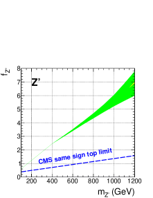
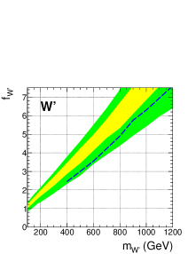
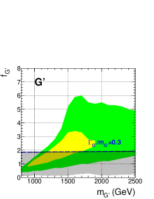
Figure 1 shows the results of our fits for the three models. We simulate the models using MadGraph5 Alwall et al. (2011). The yellow (green) band is the parameter space which fits the Tevatron $t\bar{t}$ total cross section and $A_{FB}^{t}$ within $1(2)\sigma$. For the $Z^{\prime}$ model, there is no allowed parameter space when $m_{Z^{\prime}}$ is less than about $400~{}{\rm GeV}$, and only a tiny region can fit within $1\sigma$ when $m_{Z^{\prime}}$ is heavier than $1100~{}{\rm GeV}$, with large couplings $f_{Z^{\prime}}\gtrsim 6.6$ . This conclusion differs from the one in our earlier work. The difference comes entirely from the fact that we are now fitting the most recent CDF data in which $A_{FB}^{t}$ is smaller. The contribution from $Z^{\prime}$ exchange is fed by the $u$ and $\bar{u}$ initial states which have large parton densities at the Tevatron $p\bar{p}$ collider. Therefore, both $A_{FB}^{t}$ and the $t\bar{t}$ total cross section change rapidly with the coupling $f_{Z^{\prime}}$. When $f_{Z^{\prime}}$ is large enough to bring the total cross section into a region that is consistent with data at the $2\sigma$ level, $A_{FB}^{t}$ at high $m_{t\bar{t}}~{}(\geq 450~{}{\rm GeV})$ becomes too large to fit the data. As a result, only a small parameter space yields a better fit than the SM itself, and it is very difficult to reach agreement with data within $1\sigma$. Therefore, we now conclude that the minimal flavor-changing $Z^{\prime}$ model can barely explain the large deviation of $A_{FB}^{t}$ from the SM observed at the Tevatron. In FIG. 1($Z^{\prime}$), we also plot the upper limit of the coupling for the $Z^{\prime}$ model obtained from the search of same-sign top quark pairs at the LHC Chatrchyan et al. (2012b). The region above the blue dashed curve is not allowed since too many same-sign top quark pairs would be produced. The minimal version of the $Z^{\prime}$ model is definitely disfavored.

In contrast to the $Z^{\prime}$ case, there is a large region of parameter space in which the $W^{\prime}$ model can fit the Tevatron data within $1\sigma$ and $2\sigma$, as shown in FIG. 1($W^{\prime}$). We scan the coupling $f_{W^{\prime}}$ in the $W^{\prime}$ model up to 7.5 in our numerical study. We see that the $W^{\prime}$ model can fit data quite well with $m_{W^{\prime}}\lesssim 1~{}{\rm TeV}$ for the coupling parameter $f_{W^{\prime}}\lesssim 7.5$. The asymmetry and the $t\bar{t}$ cross section do not change as sharply with coupling in the $W^{\prime}$ model as they do in the $Z^{\prime}$ case since their contributions are fed by the smaller $d$ and $\bar{d}$ parton densities. The upper limit of the coupling for the $W^{\prime}$ model is shown in the figure. We obtain this upper limit from an analysis of the CMS data on the production of a top pair plus one jet  Chatrchyan et al. (2012a). The region above the blue dashed curve is not allowed since too many $t\bar{t}+j$ events would be produced. The data were not analyzed for values of the $W^{\prime}$ mass below 400 GeV so we do not show a constraint below this value. There is a similar constraint from ATLAS Aad et al. (2012b), but we do not use the bound shown in their FIG. 6 because the interference term between the SM and the $W^{\prime}$ model is not considered in the determination of their bound. This interference is not negligible Duffty et al. (2012); Endo and Iwamoto (2012). We see that some region of the parameter space of the $W^{\prime}$ model remains open. The contribution to $A_{FB}^{t}$ at the Tevatron from top-$W^{\prime}$ associated production is not incorporated in our study since it is small at Tevatron energies owing to phase space and gluon parton distribution function suppression.

In the axigluon case, we scan $g_{l}$ and $g_{h}$ up to $8$. For simplicity, we fix $g_{l}=-g_{h}=f_{G^{\prime}}$ in Eqs.(6-7). To achieve good agreement with data at the $1\sigma$ level, the mass of axigluon is required to be in the range of about $900~{}{\rm GeV}$ to $1900~{}{\rm GeV}$. For other axigluon masses, the model can only fit data at the $2\sigma$ level. These results are shown in FIG. 1($G^{\prime}$). In FIG. 1($G^{\prime}$), we also show some bounds on axigluon masses and couplings obtained from a search for resonances in the dijet invariant mass distribution  Aad et al. (2011, 2012c); ATLAS:2012joa ; ATLAS:2012vua . To obtain the lower bound on the coupling constant $f_{G^{\prime}}$, we generate parton level dijet events in the axigluon model using MadGraph5 and MadEvent Alwall et al. (2011). After adding the cuts on the final state partons employed in Aad et al. (2011, 2012c); ATLAS:2012joa ; ATLAS:2012vua , we obtain the cross sections $\sigma\times\mathcal{A}$, where $\mathcal{A}$ represents acceptance. Comparing these results with the exclusion bound in Aad et al. (2011, 2012c); ATLAS:2012joa ; ATLAS:2012vua , we derive the lower bounds of the excluded region for $f_{G^{\prime}}$ as a function of axigluon mass, shown in FIG 1($G^{\prime}$). On the other hand, axigluons with large width cannot be excluded using the search technique described in the ATLAS paper. The contribution from a broad axigluon would cover a large fraction of the search region in the dijet invariant mass and be absorbed into the data-driven background fit. To account for this limitation of the search, we sketch a soft upper limit of the exclusion region in $f_{G^{\prime}}$ determined by the value $\Gamma_{G^{\prime}}/m_{G^{\prime}}=0.3$ (the blue shaded region in FIG. 1($G^{\prime}$)).

Before concluding this discussion of fits to the Tevatron data, we acknowledge limitations of our approach. For the three new physics models, we compare the $t\bar{t}$ forward-backward asymmetry with the unfolded data of the CDF collaboration. The unfolded result is obtained under the assumption that the events follow the SM $t\bar{t}$ event distribution, so the comparison is not exact for new physics models. The correction could be significant for $t-$channel exotic vector bosons. Indeed, the authors of Ref. Gresham et al. (2011) show that the cut efficiency is larger in the SM in the region of large $m_{t\bar{t}}$ than for the case of a $t-$channel exotic vector boson. There are two main influences of this difference Gresham et al. (2011). First, the lower efficiency of the $t-$channel new physics models, especially in the large $m_{t\bar{t}}$ region, will suppress the number of large $m_{t\bar{t}}$ events in the new physics models and release the tension between theory and data. However, in our analysis, we do not fit the differential cross section in $m_{t\bar{t}}$, only the cross section integrated over $m_{t\bar{t}}$. Since the cross section falls rapidly with $m_{t\bar{t}}$, the pertinent correction is relatively small in our fit. Second, the difference between the cut efficiencies for events with $\Delta y>0$ and $\Delta y<0$ in the new physics models will decrease the prediction of $A_{FB}^{t}$. Such effects are shown in Gresham et al. (2011) to be not as large as the cut efficiency effect on the invariant mass distribution. It is worth remarking that the NLO QCD correction for the pure new physics term and for the NP-SM interference term is larger in the large invariant mass region than in the low invariant mass region Yan et al. (2012). The NLO QCD correction will therefore counteract the cut efficiency effect at least partly. A complete investigation that includes both the NLO and cut efficiency effects is desirable, but we judge that the simpler approach used here suffices for our limited purposes.

To summarize this section, we remark that based on the latest $A_{FB}^{t}$ data from CDF at the Tevatron, the simple $Z^{\prime}$ model is disfavored, and a light $W^{\prime}$ ($\lesssim 1~{}{\rm TeV}$) is preferred for a small coupling strength, while an axigluon model can give a good fit with an axigluon mass about $1200~{}{\rm GeV}\sim 1900~{}{\rm GeV}$.

III LHC proton-proton Collider

In this section we address the charge asymmetry in rapidity $A_{C}$ measured at the LHC. We obtain estimates of LHC expectations first by simple extrapolation from the Tevatron data on $A_{FB}^{t}$ and second based on the new physics models whose parameters we determine in Sec. II.

The proton-proton LHC collider is symmetric in rapidity, and it is ambiguous to define the forward or backward region. However, the $u$ and $d$ (valence quarks inside the proton) parton densities carry, on average, a larger fraction of the momentum of the proton than the $u$ and $d$ antiquark densities (sea quarks inside the proton). With the knowledge that there is a forward-backward asymmetry in the perturbative production process for $q\bar{q}\rightarrow t\bar{t}$ production, we expect that the top quark at the LHC will be boosted in the direction of the incident quark. As a result, top quarks should accumulate in the region of large rapidity and anti-top quarks will be preferentially in the central region. Therefore, one can define an asymmetry $A_{C}$ at the LHC as

$$A_{C}=\frac{N(|y_{t}|>|y_{\bar{t}}|)-N(|y_{t}|<|y_{\bar{t}}|)}{N(|y_{t}|>|y_{\bar{t}}|)+N(|y_{t}|<|y_{\bar{t}}|)}.$$ (10)

The SM prediction including NLO EW and QCD contributions is $A_{C}=0.0115$ at $7$ TeV center-of-mass energy Kuhn and Rodrigo (2012), and the predicted value drops when the collider energy increases. The event generator MC@NLO provides a slightly different result, $A_{C}=0.006$ Aad et al. (2012d), owing to different normalization and the absence of NLO EW corrections.

Recent measurements of $A_{C}$ at the LHC have been published by the CMS and ATLAS collaborations based on data sets with $4.7~{}{\rm fb}^{-1}$ of integrated luminosity. The results from CMS Chatrchyan et al. (2012c) obtained from the lepton plus jet final state and ATLAS  Aad et al. (2012d) obtained from combining both lepton plus jet and dilepton channels are

$${\rm CMS~{}(lepton+jets):}~{}0.004\pm 0.010{\rm(stat.)}\pm 0.012{\rm(syst.)}$$

$${\rm ATLAS~{}(combined):}~{}0.029\pm 0.018{\rm(stat.)}\pm 0.014{\rm(syst.)}.$$ (11)

The ATLAS central value is an order of magnitude larger than the CMS value, but they agree within the large uncertainties in both experiments, and they are consistent with the SM prediction.

At the LHC, $t\bar{t}$ production is dominated by the gluon-gluon initial state which provides no asymmetry, and the asymmetry $A_{C}$ generated by the quark-antiquark initial state is therefore expected to be diluted substantially. An approximate estimate for the LHC asymmetry is

$$A_{C}^{t} \approx \frac{\sigma(q\bar{q}\to t\bar{t})}{\sigma(gg\to t\bar{t})+\sigma(q\bar{q}\to t\bar{t})}\times A_{FB}^{t}(q\bar{q}\to t\bar{t})\times\tilde{\varepsilon}.$$ (12)

The first term represents the fraction of the top-quark pair production cross section induced by the $q\bar{q}$ initial state which is about 17 % in the SM at 7 TeV LHC. The second term is the asymmetry induced by the $q\bar{q}$ initial state. Given that about $88\%$ of the $t\bar{t}$ production cross section in the SM comes from the $q\bar{q}$ initial state at the Tevatron, $A_{FB}^{t}(q\bar{q}\to t\bar{t})$ can be extracted from the top quark forward-backward asymmetry observed at the Tevatron; we use $A_{FB}^{t}(q\bar{q}\to t\bar{t})\approx A_{FB}^{t}/88\%$, where $A_{FB}^{t}$ is the measured top quark asymmetry. The last term $\tilde{\varepsilon}$ in Eq. (12) represents the probability of correct identification of the forward direction, namely how frequently the forward direction represents the direction of the initial state quark. This probability has to be evaluated for both the Tevatron and the LHC.

At the Tevatron, the momentum of the proton beam is chosen as the forward direction. Therefore, the probability is

$$\varepsilon^{TEV}=\frac{\sigma(q\bar{q}\to t\bar{t})_{q/P,\bar{q}/\bar{P}}}{\sigma(q\bar{q}\to t\bar{t})_{\rm total}},$$ (13)

where the denominator is the total cross section of $q\bar{q}\to t\bar{t}$ and the numerator is the contribution to the total cross section when the initial state quark and antiquark come from proton and anitproton, respectively. An explicit evaluation can be obtained from the integral over parton densities:

$$\varepsilon^{TEV}(\hat{s})=\frac{\sum_{q}\int_{\hat{s}/S}^{1}f_{q/p}(x_{1})f_{\bar{q}/\bar{p}}\left(\frac{\hat{s}}{x_{1}S}\right)\frac{dx_{1}}{x_{1}}}{\sum_{q}\int_{\hat{s}/S}^{1}\left[f_{q/p}(x_{1})f_{\bar{q}/\bar{p}}\left(\frac{\hat{s}}{x_{1}S}\right)+f_{\bar{q}/p}(x_{1})f_{q/\bar{p}}\left(\frac{\hat{s}}{x_{1}S}\right)\right]\frac{dx_{1}}{x_{1}}},$$ (14)

where $S$ is the square of the total energy of the $\bar{p}p$ collision and $\hat{s}$ denotes the square of the energy in the partonic collison.

At the LHC, with no preferred direction in a proton-proton collider, the boost direction of the $t\bar{t}$ system is chosen to be the forward direction. Hence, the probability of choosing the forward direction correctly is

$$\varepsilon^{LHC}=\frac{\sigma(q\bar{q}\to t\bar{t})_{q>\bar{q}}}{\sigma(q\bar{q}\to t\bar{t})_{\rm total}},$$ (15)

where the numerator now is the contribution to the total cross section when the initial quark momentum is larger the initial state antiquark momentum. The corresponding integral over parton densities is

$$\varepsilon^{LHC}(\hat{s})=\frac{\sum_{q}\int_{\sqrt{\hat{s}/S}}^{1}f_{q/p}(x_{1})f_{\bar{q}/p}\left(\frac{\hat{s}}{x_{1}S}\right)\frac{dx_{1}}{x_{1}}}{\sum_{q}\int_{\hat{s}/S}^{1}f_{q/p}(x_{1})f_{\bar{q}/p}\left(\frac{\hat{s}}{x_{1}S}\right)\frac{dx_{1}}{x_{1}}}.$$ (16)

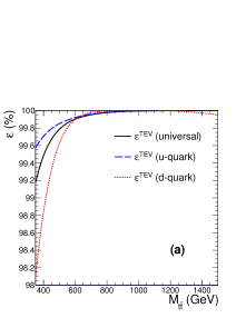
We evaluate the efficiencies explicitly using the MSTW parton distribution functions (PDFs) Martin et al. (2009). The efficiencies vary with the invariant mass of the $t\bar{t}$ system, as shown in Fig. 2. At the Tevatron, the value of $\varepsilon^{TEV}$ is nearly $100\%$, and the proton (antiproton) beam represents the direction of initial quark (antiquark) quite well. However, at the LHC, the probability $\varepsilon^{LHC}$ that the initial quark direction matches the boost direction of the $t\bar{t}$ system is lower. We find values in the range $72\%-83\%$, depending upon the initial state quark and the effective energy of the $t\bar{t}$ center mass system (FIG.  2). Since the values of $\varepsilon$’s are not $100\%$ at the LHC, the wrong choice of forward direction decreases the absolute value of $A_{FB}^{t}$.

The measured number of forward (backward) events is therefore $N_{F}\varepsilon+N_{B}(1-\varepsilon)$ ($N_{B}\varepsilon+N_{F}(1-\varepsilon)$), where $N_{F(B)}$ is the true number of events in the forward region. As a result, the measured $A_{FB}^{t}$ equals $A_{FB}^{t~{}{\text{true}}}\times(2\varepsilon-1)$. The suppression factor $\tilde{\varepsilon}$ defined in Eq. (12) is shown on the right side of Fig. 2. Its value is

$$\tilde{\varepsilon}=\frac{2\varepsilon^{LHC}-1}{2\varepsilon^{TEV}-1}\approx(54\pm 10)\%.$$ (17)

Combining all terms, we expect that $A^{t}_{C}\simeq 0.17\times A_{FB}^{t}/88\%\times 54\%\simeq 0.1A_{FB}^{t}$, where we recall that $A_{FB}^{t}$ is the value measured at the Tevatron.

Figure 2: (a) The probability for choosing the correct forward direction, the direction of initial state quark at the Tevatron. (b) The probability for choosing the correct forward direction, the direction of initial state quark at the LHC. For the “universal” case, we include all four flavors of light quarks with equal weight when we calculate $\varepsilon$. For the “$u(d)$-quark” case, we include only the contribution from the $u(d)$-quark. We do not show the behavior of other light flavors because they are sea quarks at the Tevatron and do not give a significant contribution to $A_{FB}^{t}$. (c) The relative suppression factor $\tilde{\varepsilon}$ for the universal, $u$-quark, and $d$-quark cases.

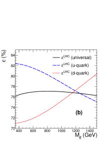
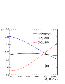
Taking $A_{FB}^{t}\sim 20\%$, we see that an extrapolation from the Tevatron provides a rough estimate for the LHC of $A_{C}\simeq 0.02$, in reasonable agreement with the central value of the ATLAS measurement but in excess of the central value of the CMS measurement. Setting aside for the moment the still large uncertainties of the LHC data, the agreement of the ATLAS measurement with our extrapolation lends credence to the suggestion that new physics contributions are playing a role in the asymmetry measured at the Tevatron. On the other hand, there is evident tension between the Tevatron asymmetry and the central value of the CMS measurement.

Our model-based predictions of $A_{C}$, to be discussed presently, provide values of $A_{C}$ a little higher than the simple extrapolation. The difference arises because the new physics contributions change the fraction of the $q\bar{q}$ initial state contribution to $t\bar{t}$ production at the Tevatron and the LHC. The SM prediction for the $\bar{t}t$ cross section is $150\pm 19\text{pb}$ Campbell et al. (2012), and the ATLAS measurement is $177\pm 3~{}({\rm stat.})^{+8}_{-7}~{}({\rm syst.})\pm 7~{}({\rm lumi.})~{}\text{pb}$  Aad et al. (2012e). In the $W^{\prime}$ and axigluon models, the contribution to $t\bar{t}$ production from new physics comes only through the $q\bar{q}$ initial state. When the new physics contribution compensates for the excess of the measured $t\bar{t}$ cross section above the SM contribution, the fraction from $q\bar{q}\to t\bar{t}$ to $t\bar{t}$ at $7~{}{\rm TeV}$ can increase to about $30\%$ compared with $17\%$ in SM. Therefore, we can expect $A_{C}\simeq 0.2A_{FB}^{t}$, a factor of 2 enhancement with respect to our previous estimate.

The analysis above provides an estimation of $A_{C}$ at the LHC from $A_{FB}^{t}$ at the Tevatron. It should be used carefully as there are reasons that it may not be good enough. First, contributions from $t\bar{t}$ processes with extra partons in the final state are not included in the estimation. They might be important for some new physics models especially for $A_{C}$ Alvarez and Leskow (2012); Drobnak et al. (2012a); Adelman et al. (2012). Second, there are models in which $A_{FB}^{t}$ at Tevatron is a residue of the balance between contributions from $u\bar{u}$ and $d\bar{d}$ initial states Drobnak et al. (2012b). In this case, $A_{C}$ at the LHC could vary over a wide range since the fraction of the $u\bar{u}$ and $d\bar{d}$ initial states is different at the LHC, and $\tilde{\varepsilon}$ for the $u$-quark and $d$-quark is different and dependent on the effective energy of the $t\bar{t}$ center of mass. Third, for new physics models in which the $A_{FB}^{t}$ results from a resonance effect, there will be a suppression (enhancement) if the resonance is heavy (light  Marques Tavares and Schmaltz (2011); Gresham et al. (2012b)).

Figure 3: The predicted top quark charge asymmetry, $A_{C}^{t}$, at the LHC at 7 TeV from the $W^{\prime}$ (left) and axigluon (right) models, compared with the ATLAS (upper) and CMS (lower) results. The inner shaded (yellow) and outer shaded (green) regions are for the couplings that fit the Tevatron $t\bar{t}$ total cross section and $A_{FB}^{t}$ within $1\sigma$ and $2\sigma$, respectively. The central value measured by ATLAS (CMS) at the LHC is marked with a (red/blue) horizontal line, and the (black) horizontal dashed lines show the $1\sigma$ uncertainty of the measurement. The irregular (blue) dashed lines on the $W^{\prime}$ figures show the bounds obtained from the analysis of top-pair-plus-one-jet events. The regions above these dashed lines are disfavored.

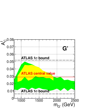
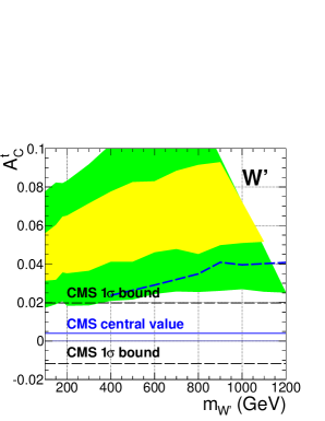
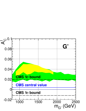
Turning next to the explicit new physics models discussed in the previous section, we use the allowed parameters for the flavor-changing $W^{\prime}$ and axigluon models shown in FIG. 1 to calculate $A_{C}$ at the LHC. The results are shown in FIG. 3, along with a comparison to results of ATLAS and CMS. We show different theory predictions for ATLAS and CMS. The difference in the assumed value of the SM contribution explains the differences in the predictions of $A_{C}$ in FIG. 3. To obtain the ATLAS predictions we use $A_{C}=0.006$ for the SM prediction, as done by ATLAS. For the CMS comparison, we use the SM value $A_{C}=0.0115$ adopted by CMS.

The values $A_{C}$ for the $W^{\prime}$ model at $7$ TeV are in the range $0.01~{}\sim 0.1$. The sharp drop for $m_{W^{\prime}}=850~{}{\rm GeV}\sim~{}1200~{}{\rm GeV}$ is related to our upper cut of the coupling parameter $g_{W^{\prime}}$ at $7.5$. Most of the values of $A_{C}$ predicted in the $W^{\prime}$ model are larger than the ATLAS central value; however, they are within the $1\sigma$ uncertainty band. For the axigluon model, all of the predictions of $A_{C}$ agree with the ATLAS result within the $1\sigma$ level. In the axigluon model $A_{C}$ does not simply increase with the axigluon coupling to SM particles. For $m_{G^{\prime}}=1500~{}{\rm GeV}$, $A_{C}$ reaches its maximum at about $4.2\%$, with coupling $f_{G^{\prime}}=2.7$. Therefore, we can see that the upper boundary of the yellow region (couplings that fit Tevatron data within $1\sigma$) overlaps the green region (couplings that fit Tevatron data within $2\sigma$) for some $m_{G^{\prime}}$. The $G^{\prime}$ model predicts smaller values of $A_{C}$ than the $W^{\prime}$ model because there is a change of the sign of the s-channel propagator. When the invariant mass of the $t\bar{t}$ system is larger than the mass of the axigluon, the contribution to $A_{C}$ from the interference term is negative. In comparing with the CMS data, we see that owing to the large contribution from new physics, the predicted values of $A_{C}$ are outside of the $1\sigma$ band. Unless the central value increases in updated measurements, the CMS data disagree with new physics models based on $W^{\prime}$ or axigluon contributions.

For the $W^{\prime}$ (and other $t-$channel new physics models), the associated production process $d(\bar{d})+g\to t(\bar{t})+W^{\prime}\to t\bar{t}+d(\bar{d})$ may also give a significant contribution to $A_{C}$. In Alvarez and Leskow (2012); Drobnak et al. (2012a), such effects are investigated for a non-self-conjugate $Z^{\prime}$ model. The large gluon parton density accentuates the cross section for a relative light $Z^{\prime}$ and $W^{\prime}$, yielding a negative contribution to $A_{C}$ Alvarez and Leskow (2012); Drobnak et al. (2012a) and releasing the tension between the small measurement at the LHC and the large predictions from the new physics models. The overlap between the predictions and the experimental bounds will be larger than shown in FIG. 3. However, a complete analysis must take into account interference between $t\bar{t}+j$ in the SM and the $W^{\prime}$ model Duffty et al. (2012); Endo and Iwamoto (2012) and a large enhancement from NLO QCD corrections ($K-$factor $\sim 1.3-1.5$ Adelman et al. (2012)) . We defer it for future study.

IV $A_{FB}^{\ell}$ and its correlation with $A_{FB}^{t}$

In addition to the top quark forward-backword asymmetry, the charge lepton asymmetry $A_{FB}^{\ell}$ is also measured by the D0 collaboration at the Tevatron and by the ATLAS collaboration at the LHC. It is defined as

$$A_{FB}^{\ell}=\frac{N_{\ell}^{+}-N_{\ell}^{-}}{N_{\ell}^{+}+N_{\ell}^{-}}.$$ (18)

At the Tevatron, $N_{\ell}^{+}$ ($N_{\ell}^{-}$) is the number of events with $q_{\ell}y_{\ell}>0$ $(q_{\ell}y_{\ell}<0)$, and $q_{\ell}$ and $y_{\ell}$ are the sign and rapidity respectively of the charged lepton from the semileptonic decay of a top or anti-top quark in the lepton plus jets events of $t{\bar{t}}$ production. As stated in the Introduction, the D0 group reports $A_{FB}^{\ell}=(11.8\pm 3.2)\%$, a deviation of about $2.2\sigma$ above the SM prediction $4.7\pm 0.1\%$ Abazov et al. (2012). At the LHC, the ATLAS collaboration measures $A_{FB}^{\ell}$ using data from the dilepton channel in $t\bar{t}$ events; $N_{\ell}^{+}$ ($N_{\ell}^{-}$) represents the number of events with $|y_{\ell^{+}}|-|y_{\ell^{-}}|>(<)0$. Based on data corresponding to $4.7~{}{\rm fb}^{-1}$ of integrated luminosity, ATLAS finds $(2.3\pm 1.2({\rm stat.})\pm 0.8({\rm syst.}))\%$, in excess of the SM prediction $0.4\%$ but within $2\sigma$ Aad et al. (2012d).

The top quark is the only quark that decays quickly, before hadronization takes place, and its polarization determines the kinematic distribution of its final state particles. Therefore, it should be possible to understand $A_{FB}^{\ell}$ based on the kinematics of the charged lepton in the decay of a top quark with different polarization states. Before presenting our numerical predictions for $A_{FB}^{\ell}$ in Sec V, we show analytically how the relationship of $A_{FB}^{\ell}$ and $A_{FB}^{t}$ is controlled by the top quark polarization. In this section, we start with the kinematics of a charged lepton in top quark decay and derive the correlation between $A_{FB}^{t}$ and $A_{FB}^{\ell}$. We introduce a variable $R_{F}$ that is useful for bridging the lepton asymmetry and the top quark asymmetry.

IV.1 Lepton kinematics and top quark polarization

The charged lepton in top quark decay is a powerful analyzer of the polarization of the top quark Mahlon and Parke (2010). Owing to the $V-A$ structure of the charged current in the SM, the angular distribution of a charged lepton $\ell^{+}$ from top quark decay ($t\to W^{+}(\to\ell^{+}\nu)b$) in the top quark rest frame is

$$\frac{1}{\Gamma}\frac{d\Gamma}{d\cos\theta_{\rm hel}}=\frac{1+\lambda_{t}\cos\theta_{\rm hel}}{2},$$ (19)

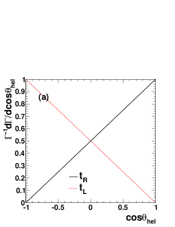
where $\lambda_{t}$ denotes the top quark helicity, and $\theta_{\rm hel}$ is the angle of $\ell^{+}$ with respect to the direction of motion of the top quark in the overall center-of-mass system of the $t\bar{t}$ production process. Throughout this paper, we use the helicity basis in our calculations. We use $\lambda_{t}=+$ to denote a right-handed top quark ($t_{R}$), and $\lambda_{t}=-$ for a left-handed top quark ($t_{L}$). The distributions are shown in FIG. 4(a). The charged lepton from a right-handed top quark decay prefers to move along the top quark direction of motion, while a lepton from a left-handed top quark moves preferentially against the top quark direction of motion. In the rest frame of the top quark, 75% (25%) of charged leptons from $t_{R}$ ($t_{L}$) decay follow the top quark direction of motion, i.e. $\cos\theta_{\rm hel}>0$.

Figure 4: (a) $\cos\theta_{\rm hel}$ distribution in the top quark rest frame for both $t_{L}$ and $t_{R}$. (b) $\cos\theta_{t\ell}$ distribution in the boosted frame for a top quark with $E_{t}=200~{}{\rm GeV}$.

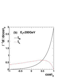
Once the top quark is boosted along its spin direction, the angular distribution of the charged lepton relative to the direction of motion of the top quark deviates from $(1\pm\cos\theta)$, and it becomes sensitive to the energy of the top quark $E_{t}$ (or equivalently its velocity $\beta$). We derive

$$\frac{d\Gamma}{\Gamma d\cos\theta_{t\ell}}=\frac{1-\beta\cos\theta_{t\ell}+\lambda_{t}\left(\cos\theta_{t\ell}-\beta\right)}{2\gamma^{2}\left(1-\beta\cos\theta_{t\ell}\right)^{3}},$$ (20)

where $\beta=\sqrt{1-m_{t}^{2}/E_{t}^{2}}$, $\gamma=E_{t}/m_{t}$ and $\theta_{t\ell}$ is the angle between the charged lepton and the direction of motion of its parent top quark. As an illustration, we plot in FIG. 4(b) the distribution of $\cos\theta_{t\ell}$ of the charged lepton for $E_{t}=200$ GeV. The leptons from both $t_{L}$ and $t_{R}$ move preferentially forward, more so for $t_{R}$ than $t_{L}$. About $60\%$ of $\ell^{+}$ follow the top quark (i.e., $\cos\theta_{t\ell}>0$ ) for $t_{L}$, and almost $100\%$ for $t_{R}$.

To obtain the forward-backward asymmetry in the laboratory frame, we must rotate the angular distribution in Eq. 20 from the top direction of motion to the laboratory coordinate axes. We use a function $R_{F}^{\ell,~{}\lambda_{t}}(\beta,y_{t})$ to represent the probability that a lepton with positive charge lands in the forward region when it originates from a top quark with velocity $\beta$, rapidity $y_{t}$, and polarization $\lambda_{t}$. Formally,

$$R_{F}^{\ell,~{}\lambda_{t}}(\beta,y_{t})=\frac{N_{F}^{\ell}}{N_{F}^{\ell}+N_{B}^{\ell}}.$$ (21)

where $N_{F}^{\ell}$ ($N_{B}^{\ell}$) denotes the number of leptons $\ell$ in the forward (backward) region in the laboratory. Moreover,

$$A_{FB}^{\ell,~{}\lambda_{t}}(\beta,y_{t})=2R_{F}^{\ell,~{}\lambda_{t}}(\beta,y_{t})-1.$$ (22)

It is noteworthy that an explicit analytic expression can be obtained for $R_{F}^{\ell,~{}\lambda_{t}}(\beta,y_{t})$ in the laboratory frame. The derivation is somewhat lengthy, and it is presented in Appendix A.3. We obtain

$$R_{F}^{\ell,\lambda_{t}}(\beta,y_{t})=\begin{cases}\displaystyle\frac{1}{2}+\frac{1}{2\left(1+\gamma^{-2}{\text{coth}}^{2}y_{t}\right)^{1/2}}+\frac{\lambda_{t}{\text{coth}}^{2}y_{t}}{4\beta\gamma^{2}\left(1+\gamma^{-2}{\text{coth}}^{2}y_{t}\right)^{3/2}}&\displaystyle y_{t}\in\left[0,~{}~{}y_{t}^{\rm max}\right]\\ &\\ \displaystyle\frac{1}{2}-\frac{1}{2\left(1+\gamma^{-2}{\text{coth}}^{2}y_{t}\right)^{1/2}}-\frac{\lambda_{t}{\text{coth}}^{2}y_{t}}{4\beta\gamma^{2}\left(1+\gamma^{-2}{\text{coth}}^{2}y_{t}\right)^{3/2}},&\displaystyle y_{t}\in\left[-y_{t}^{\rm max},~{}0\right]\end{cases}$$ (23)

where

$$y_{t}^{\rm max}=\frac{1}{2}\ln\frac{1+\beta}{1-\beta}.$$ (24)

Figures illustrating the behavior of $R_{F}^{\ell,\lambda_{t}}(\beta,y_{t})$ as a function of $y_{t}$ for different choices of $E_{t}$, and as a function of $y_{t}$ for different choices of $p_{t}$ may be found in our Ref. Berger et al. (2012b), along with a discussion of interesting kinematic features of the curves. We limit ourselves here to showing FIG. 5 and invite readers to consult our Ref. Berger et al. (2012b).

Figure 5: The ratio $R_{F}$ as a function of $y_{t}$ for a top quark with fixed energy: (a) $E_{t}=200~{}{\rm GeV}$ and (b) $E_{t}=600~{}{\rm GeV}$.

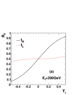
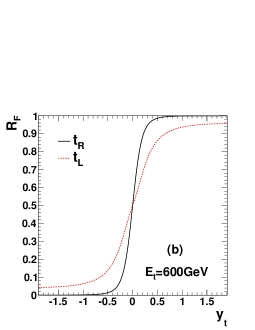
The energy $E_{t}=200~{}{\rm GeV}$ represents top quarks produced just above the threshold region, where the cross section is greatest, while $E_{t}=600~{}{\rm GeV}$ pertains to highly boosted top quarks. For right-handed top quarks $t_{R}$ (black-solid lines in FIG. 5), $R_{F}$ increases rapidly with $y_{t}$ in the region $y_{t}>0$. On the contrary, in the case of $t_{L}$’s, the ratio $R_{F}$ does not vary as significantly with $y_{t}$. For $E_{t}=200$ GeV, the boost causes charged leptons to distribute nearly uniformly, and as a result, $R_{F}$ is close to $0.5$ for the allowed range of $y_{t}$. When the energy of top quark is great enough, the large boost forces most the charged leptons from top quark decays to move along the top quark direction of motion, even for $t_{L}$.

IV.2 From $A_{FB}^{t}$ to $A_{FB}^{\ell}$

The functions $R_{F}^{\ell,~{}\lambda_{t}}(\beta,y_{t})$ in Eq. 21 and $A_{F}^{\ell,~{}\lambda_{t}}(\beta,y_{t})$ in Eq. 22 are functions of the top quark momentum. To obtain the numbers of leptons in the forward and backward regions, we must convolve $R_{F}^{\ell,~{}\lambda_{t}}(\beta,y_{t})$ with the top quark momentum spectrum on an event-by-event basis, i.e.

$$\frac{N^{\ell}_{F}}{N^{\ell}_{F}+N^{\ell}_{B}} = \frac{1}{\sigma}\sum_{\lambda=+,-}\int R_{F}^{\lambda}\left(\beta,y_{t}\right)\frac{d^{2}\sigma|_{\lambda_{t}=\lambda}}{d\beta dy_{t}}d\beta\wedge dy_{t},$$ (25)

$$\frac{N^{\ell}_{B}}{N^{\ell}_{F}+N^{\ell}_{B}} = \frac{1}{\sigma}\sum_{\lambda=+,-}\int\left[1-R_{F}^{\lambda}\left(\beta,y_{t}\right)\right]\frac{d^{2}\sigma|_{\lambda_{t}=\lambda}}{d\beta dy_{t}}d\beta\wedge dy_{t},$$ (26)

$$A_{FB}^{\ell} = \frac{1}{\sigma}\sum_{\lambda=+,-}\int\left[2R_{F}^{\lambda}\left(\beta,y_{t}\right)-1\right]\frac{d^{2}\sigma|_{\lambda_{t}=\lambda}}{d\beta dy_{t}}d\beta\wedge dy_{t}$$ (27)

where $\displaystyle{\frac{d^{2}\sigma|_{\lambda_{t}=\lambda}}{d\beta dy_{t}}}$ labels the differential $t\bar{t}$ production cross section for a top quark with specific kinematics ($\beta$, $y_{t}$, $\lambda_{t}$) and $\sigma$ stands for $t\bar{t}$ total production cross section.

The observed positive top-quark asymmetry $A_{FB}^{t}$ indicates that more top quarks are produced in the forward region than in the backward region of rapidity. Both $t_{R}$ and $t_{L}$ can generate a positive lepton asymmetry $A_{FB}^{\ell}$ from a positive $A_{FB}^{t}$. However, a $t_{L}$ would need a large boost along the proton beam line (i.e. in the large forward rapidity region) to overcome the fact that most of the charged leptons from its decay move against it in its rest frame. A right-handed top quark $t_{R}$ can yield a positive $A_{FB}^{\ell}$ even for top quarks near the $t\bar{t}$ threshold region. Therefore, the large positive top quark and lepton asymmetries $A_{FB}^{t}$ and $A_{FB}^{\ell}$ observed by the D0 collaboration indicate that the top quark polarization and the kinematics of the top quarks, $y_{t}$ and $E_{t}$, may be playing a non-trivial role.

In the SM, the vector coupling of gluons in the SM leads to equal production of left-handed and right-handed top quarks in the final state. After performing the convolutions in Eq. 27, we obtain

$$\frac{A_{FB}^{\ell}}{A_{FB}^{t}}\simeq\frac{(0+0.8)}{2}=40\%$$ (28)

in the SM at Tevatron. The first term in the numerator is the contribution from left-handed top quarks, and the second term is from the right-handed top quarks. This estimate agrees well with explicit NLO calculations Abazov et al. (2011).

This SM expectation may be contrasted with the value

$$\frac{A_{FB}^{\ell}}{A_{FB}^{t}}=(78\pm 33)\%$$ (29)

obtained from the D0 measurements of $A_{FB}^{t}$ and $A_{FB}^{\ell}=(15.2\pm 4.0)\%$ measured in the $\ell$+jets final states Abazov et al. (2011). On the other hand, using the value $A^{\ell}_{\rm FB}=(11.8\pm 3.2)\%$ obtained from a combination of measurements in the dilepton final states from $t\bar{t}$ production and the $\ell$+jets final states, we find

$$\frac{A_{FB}^{\ell}}{A_{FB}^{t}}=(60\pm 26)\%$$ (30)

The uncertainties are large, but the central values of these ratios exceed the SM estimate and indicate that the physics responsible for the forward-backward asymmetry produces more right-handed than left-handed top quarks. It would be valuable to confirm the measurement of $A_{FB}^{\ell}$ with the full data sample in D0 and to make a similar measurement with CDF data.

The top quark asymmetry $A_{FB}^{t}$ can be expressed as a sum of contributions from the SM and NP as:

$$A_{FB}^{t} = \frac{(N_{F}^{\rm NP}+N_{F}^{\rm SM})-(N_{B}^{\rm NP}+N_{B}^{\rm SM})}{(N_{F}^{\rm NP}+N_{F}^{\rm SM})+(N_{B}^{\rm NP}+N_{B}^{\rm SM})}$$ (31)

$$= A_{FB}^{t,~{}{\rm NP}}\times R^{\rm NP}+A_{FB}^{t,~{}{\rm SM}}\times(1-R^{\rm NP}),$$

where

$$A_{FB}^{t,~{}{\rm SM}}=\frac{N_{F}^{\rm SM}-N_{B}^{\rm SM}}{N_{F}^{\rm SM}+N_{B}^{\rm SM}},~{}~{}A_{FB}^{t,~{}{\rm NP}}=\frac{N_{F}^{\rm NP}-N_{B}^{\rm NP}}{N_{F}^{\rm NP}+N_{B}^{\rm NP}},~{}~{}R^{\rm NP}=\frac{N_{\rm tot}^{\rm NP}}{N_{\rm tot}^{\rm SM}+N_{\rm tot}^{\rm NP}},$$ (32)

with $N_{F(B)}^{\rm SM}$ and $N_{F(B)}^{\rm NP}$ being the numbers of events in which the top quark moves with $y_{t}>0(y_{t}<0)$ in the SM and induced by NP, respectively, and $N_{\rm tot}^{\rm SM(NP)}$ is the total number of events predicted in the SM (induced by NP).

A simplified analysis the correlation between $A_{FB}^{t}$ and $A_{FB}^{\ell}$ in presented in our Ref. Berger et al. (2012b) in which we assume that $A_{FB}^{t}$ is generated entirely by new physics. In the explicit numerical predictions presented in the next section all SM contributions including the NLO QCD effects are retained.

V $A_{FB}^{\ell}$ and new physics models: axigluon and $W^{\prime}$

Figure 6: Upper two panels: correlation between $A_{FB}^{\ell}$ and $A_{FB}^{t}$ for the $W^{\prime}$ (left) and axigluon (right) models at the Tevatron. Different colors of dots indicate different mass ranges. In the $W^{\prime}$ model, red: $100~{}{\rm GeV}\sim 300~{}{\rm GeV}$, green: $400~{}{\rm GeV}\sim 500~{}{\rm GeV}$, blue: $600~{}{\rm GeV}\sim 800~{}{\rm GeV}$, yellow:$>800~{}{\rm GeV}$. In the axigluon model, red: $800~{}{\rm GeV}\sim 1300~{}{\rm GeV}$, green: $1400~{}{\rm GeV}\sim 1700~{}{\rm GeV}$, blue: $1800~{}{\rm GeV}\sim 2100~{}{\rm GeV}$, yellow:$>2200~{}{\rm GeV}$. The (blue) square point is the D0 data $A^{\ell}_{\rm FB}={11.8\pm 3.2}\%$ with its $1\sigma$ uncertainty. The (red) vertical line shows $A_{FB}^{t}$ measured by CDF in the $8.7~{}{\rm fb}^{-1}$ data set, and the two vertical (black) lines present the $1\sigma$ uncertainty band. Lower two panels: the correlation between $A_{C}^{t}$ and $A_{C}^{\ell}$ at the LHC for the $W^{\prime}$ (left) and axigluon models (right). The vertical (horizontal) red line and the two black dashed lines show the central value of $A_{C}^{t}$ ($A_{C}^{\ell}$) and the $1\sigma$ uncertainty bands measured by ATLAS at the LHC.

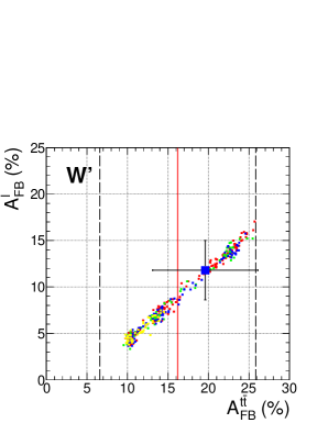
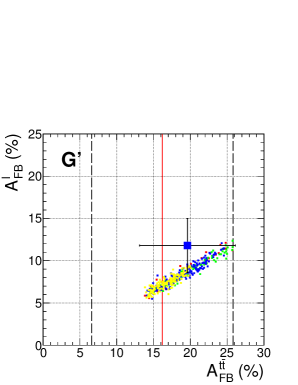
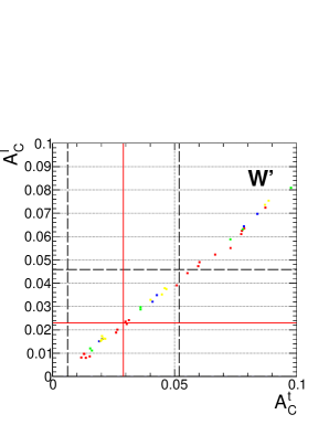
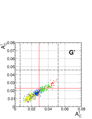
The correlation between the charged lepton asymmetry and the top quark asymmetry is significantly different for different polarization states of the top quark, and it may therefore shed light on the nature of the physics that causes the forward-backward asymmetries at the Tevatron. In this section, as in our previous study Berger et al. (2012b), we choose the $W^{\prime}$ and axigluon models as two reference models to examine the correlation at the Tevatron and the LHC. The results we show here for the Tevatron are slightly different from our previous results because we now use parameters obtained in Sec II from our fit to the CDF $8.7{\rm fb}^{-1}$ data set. In addition, we present predictions for the LHC.

The axigluon and $W^{\prime}$ models admit good fits to $A_{FB}^{t}$ at the Tevatron, but they provide distinct predictions for the polarization and kinematics of the final state top quark. The $W^{\prime}$ model produces dominantly $t_{R}$ while the axigluon model generates an equal number of $t_{R}$ and $t_{L}$ with more energetic top quarks since the quarks come from the decay of a heavy axigluon. In FIG. 6, we show the results of our calculation of the charged lepton asymmetry using the parameters determined in our $1\sigma$ fits to the $t\bar{t}$ total cross section and the most recent CDF data on $A_{FB}^{t}$ ($A_{FB}^{t}(m_{t\bar{t}}<450{\text{GeV}}),~{}A_{FB}^{t}(m_{t\bar{t}}>450{\text{GeV}})$ and $A_{FB}^{t}$). The upper two plots show the charged lepton asymmetry as a function of the top quark asymmetry at the Tevatron. The lower two plots display the charged lepton asymmetry for the LHC together with the top quark charge asymmetry $A_{C}^{t}$. For the Tevatron, the values of $A_{FB}^{t}$ are determined in the $t\bar{t}$ rest frame whereas, for comparison with the D0 point shown, $A_{FB}^{\ell}$ is in the laboratory frame. For the LHC predictions, both at $A_{C}^{t}$ and at $A_{C}^{l}$ are in the same frame.

There are vertical red lines in FIG. 6 at $A_{FB}^{t}\sim 16\%$ in the Tevatron plots and at $A_{C}^{t}\sim 0.03$ in the LHC plots to show the central values of the asymmetries measured by CDF and ATLAS, respectively, and two black dashed lines in the upper and lower plots to show the extent of the quoted experimental $1\sigma$ uncertainty bands. The horizontal red line in the LHC plots shows the central value of $A_{C}^{\ell}$ measured by ATLAS at the LHC, and the horizontal black dashed lines show the $1\sigma$ uncertainty values. Since the CDF collaboration does not present the charged lepton asymmetry $A_{FB}^{\ell}$, we show only the D0 data $A^{\ell}_{\rm FB}=(11.8\pm 3.2)\%$ as a blue square point.

The calculated charged lepton asymmetries stretch out over a range of values depending on the values of the axigluon or $W^{\prime}$ masses used in the fits to the Tevatron data. At the Tevatron, the charged lepton asymmetry spreads from $3\%$ to $17\%$ in $W^{\prime}$ the model, and over a narrower range, from $6\%$ to $13\%$ in the axigluon model. The D0 data point is in agreement with both models within uncertainties. At the LHC, there are parameters in both models (obtained from the Tevatron fits) that can reproduce the values of $A_{C}^{t}$ and $A_{C}^{\ell}$ measured at the LHC by ATLAS, shown by the fact that the intersection of the vertical and horizontal red passes through the scattering of dots. On the other hand, there is a wide range of dots in the $W^{\prime}$ model that are above the central values of $A_{C}^{t}$ and $A_{C}^{\ell}$, and out of the $1\sigma$ uncertainty band. In the axigluon model, all the values of $A_{C}^{t}$ and $A_{C}^{\ell}$ are consistent with ATLAS measurements within the $1\sigma$ bands. It is evident that LHC and Tevatron data together could reduce the allowed parameter spaces of the two models.

The best fits to the lines of points in FIG. 6 at the Tevatron are

$$A_{FB}^{\ell}=0.77\times A_{FB}^{t}-3.6\%~{}(W^{\prime});~{}~{}A_{FB}^{\ell}=0.50\times A_{FB}^{t}-1.0\%~{}({\rm axigluon}).$$ (33)

For LHC, the best fits are

$$A_{C}^{\ell}=0.85\times A_{C}^{t}-0.002~{}(W^{\prime});~{}~{}A_{C}^{\ell}=0.61\times A_{C}^{t}+0.0008~{}({\rm axigluon}).$$ (34)

Figure 7: Two-dimensional differential distribution, $(N^{t}(p_{t},y_{t})-N^{t}(p_{t},-y_{t}))_{y_{t}>0}/N_{\rm tot}$ for (a) the $W^{\prime}$ model with $m_{W^{\prime}}=200$ GeV, and (b) the axigluon model with $m_{G^{\prime}}=1.8$ TeV. The dashed line indicates $2R_{F}-1=0.5$ for each model, with $2R_{F}-1>0.5$ $(<0.5)$ on the right- (left-) side of the curve. The coupling strengths in the new physics models are chosen so that $A_{FB}^{t}$ and $A_{FB}^{\ell}$ are accommodated.

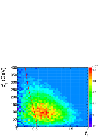
In order to gain greater insight into these correlations, we examine two-dimensional differential distributions of $A_{\rm FB}^{t}=(N_{F}^{t}-N_{B}^{t})/N_{\rm tot}$ as a function of top quark rapidity and transverse momentum. In FIG. 7 we show these density plots for a $200$ GeV $W^{\prime}$ (left) and a $1.8$ TeV $G^{\prime}$ (right) at the Tevatron. Different colors show different densities of $(N^{t}(p_{t},y_{t})-N^{t}(p_{t},-y_{t}))_{y_{t}>0}/N_{\rm tot}$. The top quark forward-backward asymmetry $A_{FB}^{t}$ is obtained after integrating over the rapidity $y_{t}$ and transverse momentum ($p_{T}^{t}$) of the top quark. As we can see, most of the events which contribute to the top quark asymmetry concentrate in the region of $p_{T}$ about $50~{}{\rm GeV}\sim 150~{}{\rm GeV}$ (the axigluon model has more events with high $p_{T}$), and $y_{t}$ about $0.4\sim 1.2$.

In FIG. 7, we also show the curve of $2R_{F}-1=0.5$ as a red dashed curve. Events to the right (left) of the curve denote values $2R_{F}-1>(<)0.5$. Note that $2R_{F}-1$ is the weight when we convolute with the differential $A_{FB}^{t}$ to obtain the charged lepton asymmetry, c.f. Eq. (27). Therefore, a larger charged lepton asymmetry is expected when there are more events to the right of the red dashed curve. In the $W^{\prime}$ model, events that contribute to $A_{FB}^{t}$ are more concentrated in the region $2R_{F}-1>0.5$ than for the axigluon model, consistent with the fact that $A_{FB}^{\ell}/A_{FB}^{t}$ in the $W^{\prime}$ model is larger than in the axigluon model.

The size of the top quark asymmetry, in excess of SM expectations, is one indication that new physics may be playing a role. The charged lepton asymmetry provides a second and independent indication of the presence of new physics since it points toward the possibility that more right- than left-handed top quarks are being produced. It is important to confirm the charged lepton asymmetry. This goal could be realized with an analysis of the full data set in D0. We also encourage the CDF collaboration to measure the charge lepton asymmetry.

VI Summary and Discussion

A forward-backward asymmetry in rapidity $A_{FB}^{t}$ of top quarks is observed at the Fermilab Tevatron. Its value exceeds SM expectations by $\sim 3\sigma$, perhaps indicative of the presence of new physics contributions in the top quark sector. In this paper we expand considerably on our previous studies of implications of the asymmetry and include new predictions for the related top quark charge asymmetry at LHC. Starting from the CDF value of $A_{FB}^{t}$ obtained in the analysis of their $8.7~{}\rm{fb}^{-1}$ data set, we derive the allowed regions parameter space of three illustrative new physics models, based, in turn, on the exchange of a flavor-changing heavy $Z^{\prime}$ or $W^{\prime}$ in the $t$-channel, or the contribution of an axigluon $G^{\prime}$ in the $s$-channel. The asymmetry data alone now show that the minimal $Z^{\prime}$ model is disfavored, a conclusion reinforced by the negative search by CMS for pairs of like-sign top quarks at the LHC. For the $W^{\prime}$ and $G^{\prime}$ models, we show that the parameter space allowed by the asymmetry data is constrained further by LHC searches for $t\bar{t}$ plus one jet events and for enhancements in the dijet mass distribution, respectively. More sophisticated models can certainly be devised as extensions of the simple $Z^{\prime}$, $W^{\prime}$, and axigluon $G^{\prime}$ models considered here. Our conclusions are limited to the models defined in Sec. II.

Our analysis of the Tevatron data is then used to obtain predictions for $A_{C}$ at the LHC. First, the association of the asymmetry $A_{FB}^{t}$ with the quark-antiquark initial state allows us, by an extrapolation in energy, to obtain an estimation of $A_{C}\simeq 0.1A_{FB}^{t}$, in agreement with the central value of the ATLAS measurement but in excess of the central value of the CMS data. Explicit calculations of $A_{C}$ based on the allowed parameter space of the $W^{\prime}$ and $G^{\prime}$ models are shown in Fig. 3 and compared with the LHC measurments by ATLAS and CMS. These calculations confirm that it is difficult to reconcile the CMS measurements of $A_{C}$ with the parameters determined from fits to $A_{FB}^{t}$ at the Tevatron. On the other hand, the ATLAS data are readily accommodated. The available LHC data on $A_{C}$ are based on a sample with only $4.7~{}\rm{fb}^{-1}$ of integrated lumiosity. A reduction of the experimental uncertainties could justify stronger conclusions regarding the compatibility of the Tevatron and LHC measurements, and a combined analysis of full statistics data from both colliders would offer significant advantages.

As discussed in Sec. II, we fit Tevatron data on the inclusive total cross section for $t\bar{t}$ production and $A_{FB}^{t}$ in order to determine the parameters of the new physics models under consideration, explaining the reasons we do not include data on the differential cross section in the invariant mass $m_{t\bar{t}}$ (see, in particular, the paragraph immediately following Eq. (9) and the next-to-last paragraph of the same section). More recent measurements of the $m_{t\bar{t}}$ distribution at the LHC by the ATLAS ATLAS:2013aa and CMS CMS:2013aa ; CMS:2013ab collaborations invite consideration of a different approach from ours, in which data from the Tevatron and the LHC are used in a joint fit to determine model parameters. The inclusion of differential data could provide further constraints on the allowed parameters of models of new physics. No excess beyond the prediction of the SM is observed in the region of large $m_{t\bar{t}}$ in the LHC data, suggesting stringent limitations on models that predict an increase in the $t\bar{t}$ rate at high $m_{t\bar{t}}$. This constraint is investigated in Refs. Aguilar-Saavedra and Perez-Victoria (2011c, c) where the cross section $\sigma\left(m_{t\bar{t}}>1{\text{TeV}}\right)$ is required to remain within 50% of its SM value. The $Z^{\prime}$ model is shown to be further excluded by this requirement, while the $W^{\prime}$ model is constrained with a tiny positive contribution to $A_{FB}^{t}$. For an $s$-channel axigluon model, our results in Sec. II show that dijet searches at the LHC exclude a narrow width axigluon whose mass is in the range [800 GeV, 2500 GeV]. Moreover, as we mention, there are subtleties in the use of the $m_{t\bar{t}}$ distribution in attempts to constrain a $G^{\prime}$ with broad width.

Once statistical precision improves sufficiently at large values of $m_{t\bar{t}}$, there is no doubt that fits to the differential distribution in $m_{t\bar{t}}$ should be done. However, we caution again that a thorough analysis would require computation of the new physics contributions at NLO, include the effects of parton showering, and take into account experimental acceptance cuts whose effects are particularly significant at large values of $m_{t\bar{t}}$ (c.f., Ref Gresham et al. (2011)). The analysis in terms of new physics models is also complicated by the fact that data on the $m_{t\bar{t}}$ distribution are unfolded in terms of the SM shape and cut efficiencies. When considering models more sophisticated than those we use here for illustrative purposes, one should bear in mind that the ultraviolet (UV) completion of the effective model can include the introduction of new particles that affect the reliable prediction of the large mass tail of the $m_{t\bar{t}}$ distribution (see, for example Ref. Ko et al. (2012a, b, c, d, e)). We readily acknowledge the value of the differential distribution in $m_{t\bar{t}}$ for constraints on models, but we defer this study to future work.

In addition to the top quark asymmetry, the charged lepton forward-backward asymmetry $A_{FB}^{\ell}$ is also measured at the Tevatron. The D0 collaboration reports $A^{\ell}_{\rm FB}=(11.8\pm 3.2)\%$, about 2.2 standard deviations above the SM value. In Sec.IV and in the Appendix, we explain the kinematic and dynamic aspects of the relationship between the asymmetries $A_{FB}^{t}$ and $A_{FB}^{\ell}$ based on the $(V-A)$ spin correlation between charged leptons and different polarization states of the top quark. We show that $A_{FB}^{\ell}$ and $A_{FB}^{t}$ are strongly positively correlated for right-handed top quarks. For left-handed top quarks, the strength of the correlation depends on how much the top quark is boosted. Since most of the $t\bar{t}$ events are produced in the threshold region, the positive values of $A_{FB}^{t}$ and $A_{FB}^{\ell}$ measured at D0 indicate that more right-handed than left-handed top quarks are being produced, in contrast to the SM expectation of equal rates. This is a second manifestations of disagreement of asymmetry data with the SM, independent of the discrepancy of the magnitude of $A_{FB}^{t}$. We hasten to remark, however, that the current uncertainties are large. The reported D0 data are based on only about half the recorded data set. Analysis of the full D0 data set is desirable, and it would be helpful to have an independent measurement of $A_{FB}^{\ell}$ from the CDF collaboration. There is great value in making measurements of both $A_{FB}^{t}$ and $A_{FB}^{\ell}$ because their correlation can be related through top quark polarization to the underlying dynamics of top quark production.

In Sec. V, we present predictions for the correlation of $A_{FB}^{\ell}$ with $A_{FB}^{t}$ at the Tevatron, and for the charged lepton asymmetry $A_{C}^{\ell}$ with the top quark asymmetry $A_{C}^{t}$ at the LHC. These predictions are based on the allowed parameter space of the two benchmark new physics models, the $W^{\prime}$ and $G^{\prime}$ models, determined from our fit to the CDF data on $A_{FB}^{t}$. In the case of both models, the allowed parameters produce a range of values for the ratios $A_{C}^{\ell}/A_{C}^{t}$ at the LHC and $A_{FB}^{\ell}/A_{FB}^{t}$ at the Tevatron, aligned along approximately straight lines in plots of $A_{C}^{\ell}$ vs $A_{C}^{t}$ and $A_{FB}^{\ell}$ vs $A_{FB}^{t}$. Ideally, precise data would provide a definite point in the two dimensional plot and tightly constrain the parameter space. The two benchmark models we consider are illustrative of the spectrum of possibilities in that the axigluon model produces an equal number of right-handed and left-handed top quarks, wheres the flavor-changing $W^{\prime}$ model produces dominantly right-handed top quarks.

As a final point, we remark that the definitions of the asymmetries require a specification of the reference frame in which they are measured, whether the laboratory frame or the $t\bar{t}$ rest frame. In this paper, we begin with $A_{FB}^{t}$ in the $t\bar{t}$ rest frame since the highest statistics value of $A_{FB}^{t}$ is measured by CDF in the $t\bar{t}$ rest frame at the Tevatron. On the other hand, the only Tevatron data on $A_{FB}^{\ell}$ are measured by D0 in the lab frame. To take frame dependence into account, one could begin from

$$\frac{A_{FB}^{\ell}(lab)}{A_{FB}^{t}(t\bar{t})}=\frac{A_{FB}^{\ell}(lab)}{A_{FB}^{t}(lab)}\frac{A_{FB}^{t}(lab)}{A_{FB}^{t}(t\bar{t})}.$$ (35)

The boost tends to reduce $A_{FB}^{t}$ in laboratory frame relative to the $t\bar{t}$ frame  Antunano et al. (2008). The reduction is about $30\%$ for the SM, but may be different when new physics is included since the kinematics of $t\bar{t}$ change slightly. As a result, $A_{FB}^{\ell}(lab)/A_{FB}^{t}(t\bar{t})$ will be smaller than $A_{FB}^{\ell}(lab)/A_{FB}^{t}(lab)$. Rather than apply uncertain correction factors, we use the D0 laboratory frame data on $A_{FB}^{\ell}$, but we urge the D0 collaboration to measure their $A_{FB}^{t}$ in the laboratory frame in order to have a more transparent comparison with new physics predictions. A better comparison with theoretical expectations of the correlation between the charged lepton asymmetry and top quark asymmetry would be possible with a D0 update of $A_{FB}^{\ell}$ and $A_{FB}^{t}$ in the same frame with their full data set.

Appendix A Energy and angular distributions of the charged lepton

We present our detailed calculation of the energy and angular distributions of the charged lepton from the decay $t\rightarrow W^{+}b\rightarrow b\ell^{+}\nu$.

A.1 The charged-lepton distributions

In the top quark rest frame, the energy and angular distribution of the charged lepton $\ell^{+}$ is

$$\frac{d\Gamma}{dxdz} = \frac{\alpha_{W}^{2}m_{t}}{32\pi AB}x(1-x)\frac{1+\lambda_{t}z}{2}{\rm Arctan}\left[\frac{Ax}{B-x}\right],$$ (36)

where $x\equiv 2E_{\text{$\ell$}}/m_{t}$ ($E_{\ell}$ is the energy of the charged lepton) and $z\equiv\cos\theta$. The angle $\theta$ is the angle between the direction of motion of the lepton and the top quark spin direction, $\lambda_{t}$ denotes the helicity of the top-quark ($\lambda_{t}=+$ for a right-handed top-quark while $\lambda_{t}=-$ for a left-handed top-quark), $A=\Gamma_{W}/m_{W}$ and $B=m_{W}^{2}/m_{t}^{2}$. The function $\rm Arctan$ is defined as

$${\rm Arctan}(x) = \begin{cases}\arctan x,&x\geqslant 0,\\ \pi+\arctan x,&x<0.\end{cases}$$

Taking the narrow width approximation for the $W$, we have

$$\frac{d\Gamma}{dxdz} = \frac{\alpha_{W}^{2}m_{t}}{32AB}~{}x(1-x)\frac{1+\lambda_{t}z}{2}~{}\Theta(x-B),$$ (37)

where $\Theta(x)$ is the Heaviside step function, and $\Theta(x-B)$ ensures the top quark decays into an on-shell $W$-boson.

Note that the energy distribution and the angular distribution are separable functions in the top quark rest frame. This implies that, after an integration over the angular distribution, the energy distributions of the leptons are identical from left-handed and right-handed top quarks.

A.2 $R_{F}$ along the direction of motion of a boosted top-quark

We consider next a boost of the top quark along its helicity axis with a velocity $\beta$. As a result of the boost, the angular $z$ and energy $x=2E_{\ell}/E_{t}$ distributions of the lepton become correlated.

Figure 8: Illustration of the charged lepton distribution from a boosted top quark in the laboratory frame. The top quark is moving along the $\hat{z}$-axis. The white inner region is not allowed for an on-shell $W$-boson. The four black-bold points along the $\hat{z}$ axis show the limits of integration of the charged-lepton energy ratio $x$.

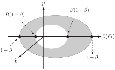
The lepton momentum and angular distribution in this new frame of reference is

$$\frac{d\Gamma}{dxdz} = \frac{\alpha_{W}^{2}m_{t}}{64AB}\frac{x}{1-\beta^{2}}\left[1-\frac{x}{1-\beta^{2}}(1-z\beta)\right]\left(1+\lambda_{t}\frac{z-\beta}{1-z\beta}\right)\Theta\left(x-\frac{B(1-\beta^{2})}{1-z\beta}\right).$$ (38)

Since the lepton’s energy spectrum cannot be negative, the upper limit of the integration over $x$ is determined by the following condition

$$1-\frac{x}{1-\beta^{2}}(1-z\beta)\geq 0,\qquad{\rm i.e.}\qquad x_{\rm max}=\frac{1-\beta^{2}}{1-z\beta}.$$ (39)

The lower limit is fixed by the Heaviside function in Eq. 38,

$$x_{\rm min}=B\frac{1-\beta^{2}}{1-z\beta}.$$ (40)

Figure 8 shows the lepton distribution along the direction of motion of the top-quark $\hat{z}(\vec{p}_{t})$ in the boosted frame. The intercepts along the $\hat{z}$-axis (i.e. the four black-bold points) are determine by the upper and lower limits of $x$ stated above. Only the shaded region is allowed by kinematics, and the inner white region is excluded by the on-shell condition of the $W$-boson. The angular distribution of the charged lepton is

$$\frac{d\Gamma}{dz}=\int^{x_{\rm max}}_{x_{\rm min}}\frac{d\Gamma}{dzdx}dx=\frac{\alpha_{W}^{2}m_{t}\left(1-B\right)^{2}\left(1+2B\right)\left(1-\beta^{2}\right)\left[1-z\beta+\lambda_{t}\left(z-\beta\right)\right]}{384AB\left(1-z\beta\right)^{3}},$$ (41)

from which we obtain the normalized angular distribution:

$$\frac{1}{\Gamma}\frac{d\Gamma}{dz}=\frac{(1-\beta^{2})\left[1-z\beta+\lambda_{t}(z-\beta)\right]}{2(1-z\beta)^{3}}.$$ (42)

Along the direction of motion of the top quark, the charged lepton is in the forward region with $z=\cos\theta>0$ and in the backward region with $z=\cos\theta<0$. The partial width of the charged lepton in the forward region is

$$\Gamma_{F} = \int_{0}^{1}\frac{d\Gamma}{dz}dz=\frac{\alpha_{W}^{2}m_{t}}{384AB}(1-3B^{2}+2B^{3})(1+\beta)\left[1+\frac{\lambda_{t}}{2}(1-\beta)\right],$$ (43)

and the partial width of the charged lepton in the backward region is

$$\Gamma_{B} = \int_{-1}^{0}\frac{d\Gamma}{dz}dz=\frac{\alpha_{W}^{2}m_{t}}{384AB}(1-3B^{2}+2B^{3})(1-\beta)\left[1-\frac{\lambda_{t}}{2}(1+\beta)\right].$$ (44)

The forward fraction ratio $R_{F}$ is

$$R_{F}=\frac{\Gamma_{F}}{\Gamma_{F}+\Gamma_{B}}=\frac{1+\beta}{4}\left[2+\lambda_{t}(1-\beta)\right].$$ (45)

Since $\beta\leq 1$, $R_{F}$ for a right-handed top quark is always larger than 75%. On the other hand, for left-handed top quarks, the leptons tend to move opposite the direction of the boost in the top quark rest frame. Owing to this anti-boost effect, there is a critical point of $R_{F}=50\%$ for a left-handed top quark. The critical point occurs at $\beta=\sqrt{2}-1\approx 0.414$, i.e. $E_{t}\approx 191.5~{}{\rm GeV}$.

A.3 $R_{F}$ in the laboratory frame

The direction of motion of a top quark does not generally coincide with the beam direction, and, therefore, the ratio $R_{F}$ derived in the previous section does not describe the probability of finding a charged lepton in the forward region of the detector. In this section we generalize $R_{F}$ to the situation in which the top quark kinematics in the laboratory frame are described by its velocity $\beta$ and rapidity $y_{t}$, or equivalently, by its traverse momentum $p_{T}$ and rapidity $y_{t}$. To obtain $R_{F}$, we will rotate the lepton momentum and angular distribution in Eq. 38 to the laboratory frame and then integrate over the forward hemisphere in this laboratory frame.

Figure 9 illustrates the charged lepton distribution in the laboratory frame whose axes are labeled $(\hat{X},\hat{Y},\hat{Z})$. The top quark boost is along its helicity axis $\hat{\eta}$. The calculation of the decay distribution of the lepton can be carried out in the new frame $(\hat{\xi},\hat{\zeta},\hat{\eta})$. The angle between $\hat{\eta}$ and $\hat{Z}$ is denoted $\Theta$, with $k\equiv-\tan\Theta$. For simplicity we require one common transverse direction for the two frames, $\hat{X}$ and $\hat{\xi}$. The important point to make is that the transverse plane $P$ ($\hat{X}$-$\hat{Y}$), which separates the forward ($Z>0$) and backward ($Z<0$) regions in the laboratory, is not perpendicular to the direction of motion of the top quark. Our task is to calculate the fraction of the charged leptons that fall in the forward region $Z>0$.

Figure 9: Illustration of the charged lepton distribution from a boosted top quark in the laboratory frame. The capital $X,Y,Z$ axes denote the laboratory frame, with the $Z$-axis being the direction of the beam line. The top quark is boosted along the $\eta$-axis.

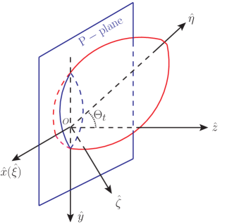
The major semi-axis of the decay ellipsoid is the $\eta$-axis direction, with focus at the origin of the two coordinate systems, the top quark decay coordinate frame and the laboratory frame. The $\xi$-axis lies in the transverse plane $P$, and the relationship of the values of $\eta$ and $\zeta$ for points in this plane is given by the equation of the line obtained by projecting the $eta$ and $zeta$ axes onto plane $P$.

$$\eta=k\zeta,~{}k<0.$$ (46)

We introduce polar coordinates,

$$\xi=\sin\theta\cos\phi,~{}\zeta=\sin\theta\sin\phi,~{}\eta=\cos\theta,$$ (47)

where $\theta$ is the polar angle, and $\phi$ is the azimuth angle in the frame $(\hat{\xi},\hat{\zeta},\hat{\eta})$. Throughout this work we choose the convention that the $\phi$ angle is in the region $[0,2\pi)$, which means $0\leq\phi<2\pi$. In terms of these polar coordinates, the equation relating points in the plane $P$ becomes

$$\cot\theta=k\sin\phi.$$ (48)

Consider the case of a top quark with positive rapidity ($k\leqslant 0$, i.e. $y_{t}\geqslant 0$). Charged leptons on the right (left) of the $P$-plane are in the forward (backward) region in the laboratory. Their momenta satisfy the conditions $\eta>k\zeta$ ($\eta<k\zeta$), respectively. In the polar coordinates, the conditions become:

$${\rm forward~{}region:}~{}~{}~{}\sin\phi>\frac{\cot\theta}{k},$$

$${\rm backward~{}region:}~{}\sin\phi<\frac{\cot\theta}{k}.$$ (49)

These two inequalities then specify the region of integration over the $\theta$ and $\phi$ angles as follows:

• $\cot\theta/k\leqslant-1$: the condition $\sin\phi>\cot\theta/k$ is always valid. Therefore, the charged lepton is always in the forward region. The integration regions are $\theta\leqslant{\rm arccot}(-k)$ and $\phi\in(0,2\pi)$.

• $\cot\theta/k\geqslant 1$ (i.e. $\theta\geqslant{\rm arccot}(k)$): there is no solution because no $\phi$ can satisfy $\sin\phi\geq\cot\theta/k\geqslant 1$.

• $-1<\cot\theta/k<1$: When $\theta>\pi/2$ ,

  $$\phi\in(\arcsin\left(\frac{\cot\theta}{k}\right),\pi-\arcsin\left(\frac{\cot\theta}{k}\right));$$ (50)

  and for $\theta\leqslant\pi/2$,

  $$\phi\in\biggl{[}0,\pi-\arcsin\left(\frac{\cot\theta}{k}\right)\biggr{)}\cup\left(2\pi+\arcsin\left(\frac{\cot\theta}{k}\right),2\pi\right).$$ (51)

We summarize the integration regions in Table 1.

Table 1: The integration regions of the $\theta$ and $\phi$ angles. Note $k<0$ by definition.

	$\cos\theta$	$\phi$
Part I	$\left(-\frac{k}{\sqrt{1+k^{2}}},1\right)$	$\left(0,2\pi\right)$
Part II	$\left(0,-\frac{k}{\sqrt{1+k^{2}}}\right)$	$\biggl{[}0,\pi-\arcsin\left(\frac{\cot\theta}{k}\right)\biggr{)}\cup\left(2\pi+\arcsin\left(\frac{\cot\theta}{k}\right),2\pi\right)$
Part III	$\left(\frac{k}{\sqrt{1+k^{2}}},0\right)$	$\left(\arcsin\left(\frac{\cot\theta}{k}\right),\pi-\arcsin\left(\frac{\cot\theta}{k}\right)\right)$
Part IV	$\left(-1,\frac{k}{\sqrt{1+k^{2}}}\right)$	$\varnothing$

The lepton spectrum from decay of the top quark is

$$\frac{d\Gamma}{dxdzd\phi} = \frac{\alpha_{W}^{2}m_{t}}{128\pi AB}\frac{x}{1-\beta^{2}}\left[1-\frac{x(1-z\beta)}{1-\beta^{2}}\right]$$ (52)

$$\times \left(1+\lambda_{t}\frac{z-\beta}{1-z\beta}\right)\Theta\left(x-\frac{B(1-\beta^{2})}{1-z\beta}\right).$$

The partial width for a lepton in the forward region is

$$\Gamma_{F} = \int_{-1}^{1}dz\int_{\frac{B(1-\beta^{2})}{1-z\beta}}^{\frac{(1-\beta^{2})}{1-z\beta}}dx\int_{\phi_{min}}^{\phi_{max}}\frac{d\Gamma}{dxdzd\phi}d\phi$$ (53)

$$= \int_{-\frac{k}{\sqrt{1+k^{2}}}}^{1}dz\int_{\frac{B(1-\beta^{2})}{1-z\beta}}^{\frac{(1-\beta^{2})}{1-z\beta}}dx\frac{2\pi d\Gamma}{dxdzd\phi}+\int_{\frac{k}{\sqrt{1+k^{2}}}}^{-\frac{k}{\sqrt{1+k^{2}}}}dz\int_{\frac{B(1-\beta^{2})}{1-z\beta}}^{\frac{(1-\beta^{2})}{1-z\beta}}dx\frac{d\Gamma}{dxdzd\phi}\left[\pi-2\arcsin\left(\frac{z}{k\sqrt{1-z^{2}}}\right)\right]$$

$$= \underbrace{\int_{-\frac{k}{\sqrt{1+k^{2}}}}^{1}dz\frac{d\Gamma}{dz}}_{\displaystyle\Gamma^{(A)}_{F}}+\underbrace{\int_{\frac{k}{\sqrt{1+k^{2}}}}^{-\frac{k}{\sqrt{1+k^{2}}}}dz\frac{d\Gamma}{2\pi dz}\left[\pi-2\arcsin\left(\frac{z}{k\sqrt{1-z^{2}}}\right)\right]}_{\displaystyle\Gamma^{(B)}_{F}}.$$

The values of $\phi_{min}$ and $\phi_{max}$ are listed in the Table, and $\Gamma_{F}^{(A)}$ is

$$\frac{\Gamma_{F}^{(A)}}{\Gamma}=\frac{\left(1+\beta\right)}{4\left(\sqrt{1+k^{2}}+k\beta\right)^{2}}\times\left\{\lambda_{t}\left(1-\beta\right)+2\left[1+k^{2}\left(1+\beta\right)+k\sqrt{1+k^{2}}\left(1+\beta\right)\right]\right\}.$$ (54)

The calculation of $\Gamma_{F}^{(B)}$ involves more steps. After integrating $x$, we obtain

$$\frac{\Gamma_{F}^{(B)}}{\Gamma} = \int_{\frac{k}{\sqrt{1+k^{2}}}}^{-\frac{k}{\sqrt{1+k^{2}}}}dz\left[\pi-2\arcsin\left(\frac{z}{k\sqrt{1-z^{2}}}\right)\right]\frac{\left(1-\beta^{2}\right)}{4\pi\left(1-z\beta\right)^{3}}\left[1-\lambda_{t}\beta+\left(\lambda_{t}-\beta\right)z\right]$$

$$= \int_{-1}^{1}dt\underbrace{\left[-1+\frac{k\beta t}{\sqrt{1+k^{2}t^{2}}}-\lambda_{t}\left(\frac{kt}{\sqrt{1+k^{2}t^{2}}}-\beta\right)\right]\times\frac{k\left(1-\beta^{2}\right)\left(\pi-2\arcsin t\right)}{4\pi\left(\sqrt{1+k^{2}t^{2}}-k\beta t\right)^{3}}}_{\displaystyle{f(t)}},$$

where we change the integration variable $z$ to $t=z/(k\sqrt{1-z^{2}})$ in the second step. The integration can be done analytically, but special care is needed at the upper and lower limit where the integral is not analytically continuous. We approach the upper bound from the left and the lower limit from the right, obtaining

$$\lim_{t\to 1^{-}}\int f\left(t\right)dt = \frac{\beta}{4\sqrt{1+k^{2}\left(1-\beta^{2}\right)}}+\frac{\lambda_{t}\left(1+k^{2}\right)\left(1-\beta^{2}\right)}{8\left[1+k^{2}\left(1-\beta^{2}\right)\right]^{3/2}}-\frac{i}{2\pi}\ln\left(k\sqrt{1+k^{2}}\right),$$

$$\lim_{t\to\left(-1\right)^{+}}\int f\left(t\right)dt = -\frac{\beta}{4\sqrt{1+k^{2}\left(1-\beta^{2}\right)}}+\frac{k\sqrt{1+k^{2}}\left(1-\beta^{2}\right)+\beta}{2\left[1+k^{2}\left(1-\beta^{2}\right)\right]}-\frac{\lambda_{t}\left(1+k^{2}\right)\left(1-\beta^{2}\right)}{8\left[1+k^{2}\left(1-\beta^{2}\right)\right]^{3/2}}$$ (56)

$$+ \frac{\lambda_{t}\left(1-\beta^{2}\right)}{4\left(\sqrt{1+k^{2}}+k\beta\right)^{2}}-\frac{i}{2\pi}\ln\left(k\sqrt{1+k^{2}}\right).$$

Hence, $\Gamma_{F}^{(B)}/\Gamma$ is

$$\frac{\Gamma_{F}^{(B)}}{\Gamma} = \frac{\beta}{2\sqrt{1+k^{2}\left(1-\beta^{2}\right)}}+\frac{\lambda_{t}\left(1+k^{2}\right)\left(1-\beta^{2}\right)}{4\left[1+k^{2}\left(1-\beta^{2}\right)\right]^{3/2}}-\frac{k\sqrt{1+k^{2}}\left(1-\beta^{2}\right)+\beta}{2\left[1+k^{2}\left(1-\beta^{2}\right)\right]}$$ (57)

$$- \frac{\lambda_{t}\left(1-\beta^{2}\right)}{4\left(\sqrt{1+k^{2}}+k\beta\right)^{2}}.$$

Finally, for a top quark in the forward region, i.e. $k\leqslant 0$ or $y_{t}\geqslant 0$, the fraction of leptons in the forward region is

$$R_{F}\equiv\frac{\Gamma_{F}}{\Gamma}=\frac{1}{2}+\frac{\beta}{2\sqrt{1+k^{2}-k^{2}\beta^{2}}}+\frac{\lambda_{t}\left(1+k^{2}\right)\left(1-\beta^{2}\right)}{4\left(1+k^{2}-k^{2}\beta^{2}\right)^{3/2}},$$ (58)

For a top quark in the backward region the result is $1-R_{F}$ (choosing the opposite $k$).

We may use $k^{2}=\tan^{2}\Theta_{t}=-1+\beta^{2}{\text{coth}}^{2}y_{t}$ to make the connection to the top quark rapidity more apparent:

$$R_{F}^{\lambda_{t}}\left(\beta,y_{t}\right)=\begin{cases}\displaystyle\frac{1}{2}+\frac{1}{2\left(1+\gamma^{-2}{\text{coth}}^{2}y_{t}\right)^{1/2}}+\frac{\lambda_{t}{\text{coth}}^{2}y_{t}}{4\beta\gamma^{2}\left(1+\gamma^{-2}{\text{coth}}^{2}y_{t}\right)^{3/2}},&y_{t}\geqslant 0,\\ \displaystyle\frac{1}{2}-\frac{1}{2\left(1+\gamma^{-2}{\text{coth}}^{2}y_{t}\right)^{1/2}}-\frac{\lambda_{t}{\text{coth}}^{2}y_{t}}{4\beta\gamma^{2}\left(1+\gamma^{-2}{\text{coth}}^{2}y_{t}\right)^{3/2}},&y_{t}<0.\end{cases}$$ (59)

One could also choose $p_{T}$ (the transverse momentum of the top-quark) and $y_{t}$ as the independent kinematic variables. Using the kinematic relations

$$k=-\frac{p_{T}{\text{csch}}y_{t}}{\sqrt{m_{t}^{2}+p_{T}^{2}}},\qquad\beta=\sqrt{1-\frac{m_{t}^{2}}{m_{t}^{2}+p_{T}^{2}}\text{sech}^{2}y_{t}}$$ (60)

one can rewrite the $R_{F}$ as:

$$R_{F}^{\lambda_{t}}\left(p_{T},y_{t}\right)=\begin{cases}\displaystyle\frac{1}{2}+\frac{1}{2}\left(1+\frac{m_{t}^{2}\text{csch}^{2}y_{t}}{m_{t}^{2}+p_{T}^{2}}\right)^{-1/2}+\frac{\lambda_{t}}{4}\left(\frac{m_{t}^{2}\text{csch}^{2}y_{t}}{m_{t}^{2}+p_{T}^{2}}\right)\\ \displaystyle\qquad\times\left(1+\frac{m_{t}^{2}\text{csch}^{2}y_{t}}{m_{t}^{2}+p_{T}^{2}}\right)^{-3/2}\left(1-\frac{m_{t}^{2}\text{sech}^{2}y_{t}}{m_{t}^{2}+p_{T}^{2}}\right)^{-1/2},&y_{t}\geqslant 0,\\ \\ \displaystyle\frac{1}{2}-\frac{1}{2}\left(1+\frac{m_{t}^{2}\text{csch}^{2}y_{t}}{m_{t}^{2}+p_{T}^{2}}\right)^{-1/2}-\frac{\lambda_{t}}{4}\left(\frac{m_{t}^{2}\text{csch}^{2}y_{t}}{m_{t}^{2}+p_{T}^{2}}\right)\\ \displaystyle\qquad\times\left(1+\frac{m_{t}^{2}\text{csch}^{2}y_{t}}{m_{t}^{2}+p_{T}^{2}}\right)^{-3/2}\left(1-\frac{m_{t}^{2}\text{sech}^{2}y_{t}}{m_{t}^{2}+p_{T}^{2}}\right)^{-1/2},&y_{t}<0.\end{cases}$$

A.4 Critical Behavior of $R_{F}$

A few interesting features of the ratio $R_{F}$ are worthy of note. For left-handed top quarks, when $p_{T}$ is not large, peak structure is present in $R_{F}^{\lambda_{t}}\left(p_{T},y_{t}\right)$, and there is more than one value of $y_{t}$ which satisfies the equation $R_{F}^{\lambda_{t}}\left(\beta,y_{t}\right)=0.5$.

In principle, a peak position can be obtained by solving the equation

$$\frac{\partial R_{F}^{\lambda_{t}}\left(p_{T},y_{t}\right)}{\partial y_{t}}=0,$$ (61)

The derivative is not amenable to an analytic solution, but we can still determine the critical value of $p_{T}^{c}$. When $p_{T}>p_{T}^{c}$, there is no peak structure in $R_{F}^{\lambda_{t}}\left(p_{T},y_{t}\right)$. When $p_{T}<p_{T}^{c}$, $R_{F}^{\lambda_{t}}\left(p_{T},y_{t}\right)$ shows peak structure for left-handed top quarks. Solving

$$\frac{\partial R_{F}^{\lambda_{t}}\left(p_{T}^{c},y_{t}\right)}{\partial y_{t}}\bigg{|}_{y_{t}=0}=0,$$ (62)

to obtain $p_{T}^{c}$, we find

$$\frac{m_{t}^{2}+\left(p_{T}^{c}\right)^{2}-2p_{T}^{c}\sqrt{m_{t}^{2}+\left(p_{T}^{c}\right)^{2}}}{4m_{t}p_{T}^{c}}=0.$$ (63)

The only physical solution is $p_{T}^{c}=m_{t}/\sqrt{3}\simeq 100\text{GeV}$.

For left-handed top quarks, there are values of the boost for which the equation $R_{F}^{\lambda_{t}}\left(\beta,y_{t}\right)=0.5$ has more than one solution. In this interval of $\beta$, $R_{F}^{\lambda_{t}}\left(\beta,y_{t}\right)$ is not far from $0.5$ and is nearly constant. The solution of $R_{F}^{\lambda_{t}}\left(\beta,y_{t}\right)=0.5$ is ${\text{coth}}^{2}y_{t}=-\gamma^{2}\left(1+\frac{\lambda_{t}}{2\beta}\right)^{-1}$. Because $k^{2}=-1+\beta^{2}{\text{coth}}^{2}y_{t}$ should be greater than 0, we require ${\text{coth}}^{2}y_{t}\geqslant 1/\beta^{2}$. In the region $\beta\in\left(\sqrt{2}-1,{\displaystyle\frac{1}{2}}\right)$ we find that $R_{F}^{\lambda_{t}}\left(\beta,y_{t}\right)$ is nearly constant for left-handed top quartks. The corresponding values of the energy of the top quark are $E_{t}\in\left(191.5\text{GeV},{\displaystyle 201.3\text{GeV}}\right)$.

References

- Aaltonen et al. (2011) T. Aaltonen et al. (CDF Collaboration), Phys.Rev. D83, 112003 (2011), eprint 1101.0034.
- Abazov et al. (2011) V. M. Abazov et al. (D0 Collaboration), Phys.Rev. D84, 112005 (2011), eprint 1107.4995.
- Jung et al. (2010) S. Jung, H. Murayama, A. Pierce, and J. D. Wells, Phys.Rev. D81, 015004 (2010), eprint 0907.4112.
- Cao et al. (2010a) J. Cao, Z. Heng, L. Wu, and J. M. Yang, Phys.Rev. D81, 014016 (2010a), eprint 0912.1447.
- Xiao et al. (2010a) B. Xiao, Y.-k. Wang, and S.-h. Zhu, Phys.Rev. D82, 034026 (2010a), eprint 1006.2510.
- Cao et al. (2011) J. Cao, L. Wang, L. Wu, and J. M. Yang, Phys.Rev. D84, 074001 (2011), eprint 1101.4456.
- Berger et al. (2011) E. L. Berger, Q.-H. Cao, C.-R. Chen, C. S. Li, and H. Zhang, Phys.Rev.Lett. 106, 201801 (2011), eprint 1101.5625.
- Zhou et al. (2011) Z.-q. Zhou, B. Xiao, Y.-k. Wang, and S.-h. Zhu, Phys.Rev. D83, 094022 (2011), eprint 1102.1044.
- Aguilar-Saavedra and Perez-Victoria (2011a) J. Aguilar-Saavedra and M. Perez-Victoria, JHEP 1105, 034 (2011a), eprint 1103.2765.
- Gresham et al. (2011) M. I. Gresham, I.-W. Kim, and K. M. Zurek, Phys.Rev. D83, 114027 (2011), eprint 1103.3501.
- Aguilar-Saavedra and Perez-Victoria (2011b) J. Aguilar-Saavedra and M. Perez-Victoria, Phys.Lett. B701, 93 (2011b), eprint 1104.1385.
- Aguilar-Saavedra and Perez-Victoria (2011c) J. Aguilar-Saavedra and M. Perez-Victoria, Phys.Rev. D84, 115013 (2011c), eprint 1105.4606.
- Duraisamy et al. (2011) M. Duraisamy, A. Rashed, and A. Datta, Phys.Rev. D84, 054018 (2011), eprint 1106.5982.
- Aguilar-Saavedra and Perez-Victoria (2011c) J. Aguilar-Saavedra and M. Perez-Victoria (2011c), eprint 1107.0841.
- Gresham et al. (2012a) M. I. Gresham, I.-W. Kim, and K. M. Zurek, Phys.Rev. D85, 014022 (2012a), eprint 1107.4364.
- Ko et al. (2012a) P. Ko, Y. Omura, and C. Yu, Phys.Rev. D85, 115010 (2012a), eprint 1108.0350.
- Ko et al. (2012b) P. Ko, Y. Omura, and C. Yu, JHEP 1201, 147 (2012b), eprint 1108.4005.
- Ko et al. (2012c) P. Ko, Y. Omura, and C. Yu, Nuovo Cim. C035N3, 245 (2012c), eprint 1201.1352.
- Ko et al. (2012d) P. Ko, Y. Omura, and C. Yu, Eur.Phys.J. C73, 2269 (2013), eprint 1205.0407.
- Li et al. (2012) B. H. Li, C. S. Li, H. T. Li, Y. C. Zhan, Y. Zhang, and J. Wang, Phys.Rev. D86, 114027 (2012a), eprint 1208.0418.
- Ko et al. (2012e) P. Ko, Y. Omura, and C. Yu (2012e), eprint 1208.4675.
- Alvarez and Leskow (2012) E. Alvarez and E. C. Leskow, Phys.Rev. D86, 114034 (2012a), eprint 1209.4354.
- Drobnak et al. (2012a) J. Drobnak, A. L. Kagan, J. F. Kamenik, G. Perez, and J. Zupan, Phys.Rev. D86, 094040 (2012a), eprint 1209.4872.
- Aguilar-Saavedra and Perez-Victoria (2011c) J. Aguilar-Saavedra and M. Perez-Victoria (2013c), eprint 1302.6618.
- Cheung et al. (2009) K. Cheung, W.-Y. Keung, and T.-C. Yuan, Phys.Lett. B682, 287 (2009), eprint 0908.2589.
- Barger et al. (2010) V. Barger, W.-Y. Keung, and C.-T. Yu, Phys.Rev. D81, 113009 (2010), eprint 1002.1048.
- Cheung and Yuan (2011) K. Cheung and T.-C. Yuan, Phys.Rev. D83, 074006 (2011), eprint 1101.1445.
- Barger et al. (2011) V. Barger, W.-Y. Keung, and C.-T. Yu, Phys.Lett. B698, 243 (2011), eprint 1102.0279.
- Bhattacherjee et al. (2011) B. Bhattacherjee, S. S. Biswal, and D. Ghosh, Phys.Rev. D83, 091501 (2011), eprint 1102.0545.
- Craig et al. (2011) N. Craig, C. Kilic, and M. J. Strassler, Phys.Rev. D84, 035012 (2011), eprint 1103.2127.
- Chen et al. (2011a) C.-H. Chen, S. S. Law, and R.-H. Li, J.Phys. G38, 115008 (2011a), eprint 1104.1497.
- Cao et al. (2012) J. Cao, K. Hikasa, L. Wang, L. Wu, and J. M. Yang, Phys.Rev. D85, 014025 (2012), eprint 1109.6543.
- Yan et al. (2012) K. Yan, J. Wang, D. Y. Shao, and C. S. Li, Phys.Rev. D85, 034020 (2012), eprint 1110.6684.
- Knapen et al. (2012) S. Knapen, Y. Zhao, and M. J. Strassler, Phys.Rev. D86, 014013 (2012), eprint 1111.5857.
- Duffty et al. (2012) D. Duffty, Z. Sullivan, and H. Zhang, Phys.Rev. D85, 094027 (2012), eprint 1203.4489.
- Adelman et al. (2012) J. Adelman, J. Ferrando, and C. White, JHEP 1302, 091 (2012b), eprint 1206.5731.
- Endo and Iwamoto (2012) M. Endo and S. Iwamoto, Phys.Lett. B718, 1070 (2013), eprint 1207.5900.
- Antunano et al. (2008) O. Antunano, J. H. Kuhn, and G. Rodrigo, Phys.Rev. D77, 014003 (2008), eprint 0709.1652.
- Ferrario and Rodrigo (2008) P. Ferrario and G. Rodrigo, Phys.Rev. D78, 094018 (2008), eprint 0809.3354.
- Ferrario and Rodrigo (2009a) P. Ferrario and G. Rodrigo, Phys.Rev. D80, 051701 (2009a), eprint 0906.5541.
- Ferrario and Rodrigo (2009b) P. Ferrario and G. Rodrigo, J.Phys.Conf.Ser. 171, 012091 (2009b), eprint 0907.0096.
- Frampton et al. (2010) P. H. Frampton, J. Shu, and K. Wang, Phys.Lett. B683, 294 (2010), eprint 0911.2955.
- Cao et al. (2010b) Q.-H. Cao, D. McKeen, J. L. Rosner, G. Shaughnessy, and C. E. Wagner, Phys.Rev. D81, 114004 (2010b), eprint 1003.3461.
- Chivukula et al. (2010) R. S. Chivukula, E. H. Simmons, and C.-P. Yuan, Phys.Rev. D82, 094009 (2010), eprint 1007.0260.
- Xiao et al. (2010b) B. Xiao, Y.-k. Wang, and S.-h. Zhu (2010b), eprint 1011.0152.
- Bai et al. (2011) Y. Bai, J. L. Hewett, J. Kaplan, and T. G. Rizzo, JHEP 1103, 003 (2011), eprint 1101.5203.
- Wang et al. (2011a) X.-P. Wang, Y.-K. Wang, B. Xiao, J. Xu, and S.-h. Zhu, Phys.Rev. D83, 115010 (2011a), eprint 1104.1917.
- Marques Tavares and Schmaltz (2011) G. Marques Tavares and M. Schmaltz, Phys.Rev. D84, 054008 (2011), eprint 1107.0978.
- Alvarez et al. (2011a) E. Alvarez, L. Da Rold, J. I. S. Vietto, and A. Szynkman, JHEP 1109, 007 (2011a), eprint 1107.1473.
- Aguilar-Saavedra and Perez-Victoria (2011d) J. Aguilar-Saavedra and M. Perez-Victoria, Phys.Lett. B705, 228 (2011d), eprint 1107.2120.
- Wang et al. (2011b) H. Wang, Y.-k. Wang, B. Xiao, and S.-h. Zhu, Phys.Rev. D84, 094019 (2011b), eprint 1107.5769.
- Krnjaic (2012) G. Z. Krnjaic, Phys.Rev. D85, 014030 (2012), eprint 1109.0648.
- Aguilar-Saavedra and Santiago (2012) J. Aguilar-Saavedra and J. Santiago, Phys.Rev. D85, 034021 (2012), eprint 1112.3778.
- Gabrielli et al. (2012) E. Gabrielli, M. Raidal, and A. Racioppi, Phys.Rev. D85, 074021 (2012), eprint 1112.5885.
- Zhu et al. (2012) H. X. Zhu, C. S. Li, D. Y. Shao, J. Wang, and C. Yuan, Eur.Phys.J. C72, 2232 (2012), eprint 1201.0672.
- Cvetic et al. (2012) M. Cvetic, J. Halverson, and P. Langacker, JHEP 1211, 064 (2012b), eprint 1209.2741.
- Dutta et al. (2012) S. Dutta, A. Goyal, and M. Kumar (2012), eprint 1209.3636.
- Gross et al. (2012) C. Gross, G. M. Tavares, C. Spethmann, and M. Schmaltz, Phys.Rev. D87, 014004 (2013), eprint 1209.6375.
- Gresham et al. (2012b) M. Gresham, J. Shelton, and K. M. Zurek, JHEP 1303, 008 (2013), eprint 1212.1718.
- Djouadi et al. (2010) A. Djouadi, G. Moreau, F. Richard, and R. K. Singh, Phys.Rev. D82, 071702 (2010), eprint 0906.0604.
- Shu et al. (2010) J. Shu, T. M. Tait, and K. Wang, Phys.Rev. D81, 034012 (2010), eprint 0911.3237.
- Arhrib et al. (2010) A. Arhrib, R. Benbrik, and C.-H. Chen, Phys.Rev. D82, 034034 (2010), eprint 0911.4875.
- Dorsner et al. (2010) I. Dorsner, S. Fajfer, J. F. Kamenik, and N. Kosnik, Phys.Rev. D81, 055009 (2010), eprint 0912.0972.
- Bauer et al. (2010) M. Bauer, F. Goertz, U. Haisch, T. Pfoh, and S. Westhoff, JHEP 1011, 039 (2010), eprint 1008.0742.
- Chen et al. (2011b) C.-H. Chen, G. Cvetic, and C. Kim, Phys.Lett. B694, 393 (2011b), eprint 1009.4165.
- Alvarez et al. (2011b) E. Alvarez, L. Da Rold, and A. Szynkman, JHEP 1105, 070 (2011b), eprint 1011.6557.
- Patel and Sharma (2011) K. M. Patel and P. Sharma, JHEP 1104, 085 (2011), eprint 1102.4736.
- Zerwekh (2011) A. R. Zerwekh, Phys.Lett. B704, 62 (2011), eprint 1103.0956.
- Barreto et al. (2011) E. R. Barreto, Y. Coutinho, and J. Sa Borges, Phys.Rev. D83, 054006 (2011), eprint 1103.1266.
- Foot (2011) R. Foot, Phys.Rev. D83, 114013 (2011), eprint 1103.1940.
- Jung et al. (2011a) S. Jung, A. Pierce, and J. D. Wells, Phys.Rev. D83, 114039 (2011a), eprint 1103.4835.
- Jung et al. (2011b) S. Jung, A. Pierce, and J. D. Wells, Phys.Rev. D84, 055018 (2011b), eprint 1104.3139.
- Babu et al. (2011) K. Babu, M. Frank, and S. K. Rai, Phys.Rev.Lett. 107, 061802 (2011), eprint 1104.4782.
- Djouadi et al. (2011) A. Djouadi, G. Moreau, and F. Richard, Phys.Lett. B701, 458 (2011), eprint 1105.3158.
- Hektor et al. (2011) A. Hektor, G. Hutsi, M. Kadastik, K. Kannike, M. Raidal, et al., Phys.Rev. D84, 031701 (2011), eprint 1105.5644.
- Cui et al. (2011) Y. Cui, Z. Han, and M. D. Schwartz, JHEP 1107, 127 (2011), eprint 1106.3086.
- Frank et al. (2011) M. Frank, A. Hayreter, and I. Turan, Phys.Rev. D84, 114007 (2011), eprint 1108.0998.
- Davoudiasl et al. (2012) H. Davoudiasl, T. McElmurry, and A. Soni, Phys.Rev. D85, 054001 (2012), eprint 1108.1173.
- Jung et al. (2011c) S. Jung, A. Pierce, and J. D. Wells, Phys.Rev. D84, 091502 (2011c), eprint 1108.1802.
- Kosnik et al. (2011) N. Kosnik, I. Dorsner, J. Drobnak, S. Fajfer, and J. F. Kamenik, PoS EPS-HEP2011, 380 (2011), eprint 1111.0477.
- de la Puente (2012) A. de la Puente, JHEP 1202, 016 (2012), eprint 1111.4488.
- Wang et al. (2012) L. Wang, L. Wu, and J. M. Yang, Phys.Rev. D85, 075017 (2012), eprint 1111.4771.
- Drobnak et al. (2012b) J. Drobnak, J. F. Kamenik, and J. Zupan, Phys.Rev. D86, 054022 (2012b), eprint 1205.4721.
- Chatrchyan et al. (2012a) S. Chatrchyan et al. (CMS Collaboration), Phys.Lett. B717, 351 (2012b), eprint 1206.3921.
- Aad et al. (2012a) G. Aad et al. (ATLAS Collaboration), JHEP 1204, 069 (2012a), eprint 1202.5520.
- Chatrchyan et al. (2012b) S. Chatrchyan et al. (CMS Collaboration), JHEP 1208, 110 (2012a), eprint 1205.3933.
- Berger et al. (2012a) E. L. Berger, Q.-H. Cao, J.-H. Yu, and H. Zhang, Phys.Rev.Lett. 109, 152004 (2012a), eprint 1207.1101.
- Abazov et al. (2012) V. M. Abazov et al. (D0 Collaboration) (2012), eprint 1207.0364.
- Bernreuther and Si (2010) W. Bernreuther and Z.-G. Si, Nucl.Phys. B837, 90 (2010), eprint 1003.3926.
- Berger et al. (2012b) E. L. Berger, Q.-H. Cao, C.-R. Chen, J.-H. Yu, and H. Zhang, Phys.Rev.Lett. 108, 072002 (2012b), eprint 1201.1790.
- Krohn et al. (2011) D. Krohn, T. Liu, J. Shelton, and L.-T. Wang, Phys.Rev. D84, 074034 (2011), eprint 1105.3743.
- Falkowski et al. (2011) A. Falkowski, G. Perez, and M. Schmaltz, Phys.Rev. D87, 034041 (2013), eprint 1110.3796.
- Bernreuther and Si (2012) W. Bernreuther and Z.-G. Si, Phys.Rev. D86, 034026 (2012), eprint 1205.6580.
- Kuhn and Rodrigo (1998) J. H. Kuhn and G. Rodrigo, Phys.Rev.Lett. 81, 49 (1998), eprint hep-ph/9802268.
- Kuhn and Rodrigo (2012) J. H. Kuhn and G. Rodrigo, JHEP 1201, 063 (2012), eprint 1109.6830.
- Aaltonen et al. (2012) T. Aaltonen et al. (CDF Collaboration), CDF Conference Note 10807 (2012).
- Aaltonen et al. (2009) T. Aaltonen et al. (CDF Collaboration), CDF Conference Note 9913 (2009).
- Campbell et al. (2012) J. Campbell, K. Ellis, and C. Williams, URL http://mcfm.fnal.gov/.
- Alwall et al. (2011) J. Alwall, M. Herquet, F. Maltoni, O. Mattelaer, and T. Stelzer, JHEP 1106, 128 (2011), eprint 1106.0522.
- Aad et al. (2012b) G. Aad et al. (ATLAS Collaboration), Phys. Rev. D 86, 091103 (2012b).
- Aad et al. (2011) G. Aad et al. (ATLAS Collaboration), New J.Phys. 13, 053044 (2011), eprint 1103.3864.
- Aad et al. (2012c) G. Aad et al. (ATLAS Collaboration), Phys.Lett. B708, 37 (2012c), eprint 1108.6311.
- (103) G. Aad et al. (ATLAS Collaboration), ATLAS-CONF-2012-088 (2012).
- (104) G. Aad et al. (ATLAS Collaboration), ATLAS-CONF-2012-148 (2012).
- Aad et al. (2012d) G. Aad et al. (ATLAS Collaboration), ATLAS-CONF-2012-057 (2012d).
- Chatrchyan et al. (2012c) S. Chatrchyan et al. (CMS Collaboration), CMS-PAS-TOP-11-030 (2012c).
- Martin et al. (2009) A. Martin, W. Stirling, R. Thorne, and G. Watt, Eur.Phys.J. C63, 189 (2009), eprint 0901.0002.
-
Aad et al. (2012e)
G. Aad et al.
(ATLAS Collaboration),
https://twiki.cern.ch/twiki/pub/AtlasPublic/CombinedSummaryPlots/ (2012e). - Mahlon and Parke (2010) G. Mahlon and S. J. Parke, Phys.Rev. D81, 074024 (2010), eprint 1001.3422.
- (110) G. Aad et al. (ATLAS Collaboration), ATLAS-CONF-2013-052 (2013).
- (111) S. Chatrchyan et al. (CMS Collaboration), CMS-PAS-TOP-12-027 (2013).
- (112) S. Chatrchyan et al. (CMS Collaboration), CMS-PAS-TOP-12-028 (2013).