Gravitational waves from BH-NS binaries: Effective Fisher matrices and parameter estimation using higher harmonics
Abstract
Inspiralling black hole-neutron star (BH-NS) binaries emit a complicated gravitational wave signature, produced by multiple harmonics sourced by their strong local gravitational field and further modulated by the orbital plane’s precession. Some features of this complex signal are easily accessible to ground-based interferometers (e.g., the rate of change of frequency); others less so (e.g., the polarization content); and others unavailable (e.g., features of the signal out of band). For this reason, an ambiguity function (a diagnostic of dissimilarity) between two such signals varies on many parameter scales and ranges. In this paper, we present a method for computing an approximate, effective Fisher matrix from variations in the ambiguity function on physically pertinent scales which depend on the relevant signal to noise ratio. As a concrete example, we explore how higher harmonics improve parameter measurement accuracy. As previous studies suggest, for our fiducial BH-NS binaries and for plausible signal amplitudes, we see that higher harmonics at best marginally improve our ability to measure parameters. For non-precessing binaries, these Fisher matrices separate into intrinsic (mass, spin) and extrinsic (geometrical) parameters; higher harmonics principally improve our knowledge about the line of sight. For the precessing binaries, the extra information provided by higher harmonics is distributed across several parameters. We provide concrete estimates for measurement accuracy, using coordinates adapted to the precession cone in the detector’s sensitive band.
pacs:
04.30.–w, 04.80.Nn, 95.55.YmI introduction
Ground based gravitational wave detector networks (notably LIGO Abb04 and Virgo virgo ) are analyzing results of design-sensitivity searches for the signals expected from the inspiral and merger of double compact binaries. Abb08 ; Abb09 . For the lowest-mass compact binaries , the response of the detector to a binary merger with arbitrary masses, spins, and even eccentricity is well understood, particularly given the detectors’ limited and low sensitive frequency band Buo03 ; Buo04 ; Dam04 ; Pan04 ; Kon05 ; Buo05 ; Kon06 ; Tes07 ; Han08 ; Hin08 ; Aru09 ; Buo09 . Though this complicated signal encodes all information about the binary’s spacetime Rya95 , the amount of accessible information depends on signal strength (or signal-to-noise ratio) Jar12 . Strong signals permit high-precision tests of general relativity; fainter signals allow high-precision constraints on some binary parameters; while very faint, short signals may only constrain the binary’s mass. Qualitatively speaking, we can distinguish two configurations if they are separated by contours , where (defined in Sec. III) is the (normalized) ambiguity function or “overlap” and is the signal-to-noise ratio (SNR).
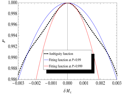
As higher-order corrections and new physics are added to our models for gravitational-wave signals, the functional dependence on various parameters (such as masses, spins and orientation angles) in the model grows in complexity. On scales , for astrophysically plausible , the ambiguity function is generally smooth. However, it may have more complicated fine-scale structure which may not be detectable for expected signal strengths. The Fisher matrix approach to estimating parameter errors is based on differentiating a waveform with respect to its parameters. These derivatives are defined in an infinitesimal patch of parameter space, and are thus measuring fine-scale structure, which could potentially be misleading about larger-scale, observable trends. This point is illustrated by Fig. 2, where we fit a quadratic through the ambiguity function. The ambiguity function changes shape, so fits to small () and large () regions of parameter space would give rather different estimates of posterior widths and thus parameter accuracy. Similarly, if the standard Fisher matrix were calculated via finite difference, step sizes on these scales would give different results, with the smaller step size giving a misleading estimate of parameter accuracy for a signal of expected strength.
In this paper we propose a simple effective procedure to identify relevant scales and parameter correlations, construct suitable “effective Fisher matrices”, and estimate ambiguity functions at low but nontrivial signal to noise ratio. To demonstrate this technique, we examine the signal from selected black hole-neutron star (BH-NS) binaries, described in Section II. In this paper we use all available knowledge about the (post Newtonian) waveform, adopting a complete model for the adiabatic quasicircular inspiral of precessing BH-NS binaries. In particular, we employ all available harmonics and amplitude corrections, introducing small but non-negligible changes to the ambiguity function. In Section III we introduce our unconventional effective approach to the local ambiguity function. Using those tools, in Section IV we construct and approximate the overlap for signals similar to each reference binary. Motivated by parameter estimation, we provide explicit expressions for the Fisher matrix, correlations, and marginalized uncertainties for each configuration. For our fiducial configurations, higher harmonics principally allow us to improve our knowledge of the binary orientation, providing fairly little additional information about intrinsic parameters for the amplitude scales of immediate astrophysical interest.
Our results are complicated by coordinate-dependent effects, notably extreme sensitivity to the reference frequency at which parameters are specified. We show the choice of reference frequency can reduce (or introduce) fine-scale structure into the ambiguity function, similar to the effect of higher harmonics. Our effective approach can partially compensate for ill-chosen coordinates, such as the coalescence phase or initial spins. To reduce but not completely eliminate these systematic effects, we express our results using parameters specified near the peak sensitivity of the detector (here, 100 Hz).
I.1 Context and prior work
Several studies of gravitational wave detection from merging binaries have employed amplitude-corrected waveforms and higher harmonics. Investigations of space-based interferometers, such as the Laser Interferometer Space Antenna (LISA), have historically used complete signal models, accounting for both spin and precession Por08 . As higher harmonics have a small effect, however, most previous studies of ground-based interferometers have omitted them, emphasizing spin. When included, higher harmonics were explored alone for non-precessing signals. Higher harmonics can allow detection of signals otherwise inaccessible due to the detector’s limited bandwidth Aru07 ; Bro07 . The relative amplitudes of higher harmonics can probe astrophysical mechanisms for generating non-circularity Key10 . Finally, higher harmonics (and precession) are well-known to break degeneracies and improve sky localization, particularly for LISA Lan06 ; Kle09 ; Lan11 .
Several authors have explored the local ambiguity function “beyond the Fisher matrix”, including higher-order correlation functions Val08 ; Vit10 and projection effects due to the local shape of the signal manifold Val11 . These methods still use explicit derivatives of the ambiguity function (via explicit derivatives of the signal) to construct their series approximations.
The Fisher matrix is often nearly or exactly singular, making inversion numerically challenging. Several authors have pointed out that a singular value implies an unconstrained parameter, limited only by the prior; see, e.g., Vallisneri Val08 . In many cases, including those singular values addressed in the text, the singular value corresponds to a bounded parameter (e.g., an angle). The singular value simply indicates that parameter cannot be measured. In the phenomenological limit described in this paper, precisely zero eigenvalues never occur, unless a parameter is constrained by symmetry.
Our goal in this work is to understand the typical shape of the posterior for a noise realization and coordinates in the signal space. Using one notion of “typical” would produce an average posterior over all noise realizations. Such an average posterior, however, could be slightly wider than the posterior from any given noise realization. Instead, in this work we attempt to characterize the typical shape of any one noise realization. To do so, in effect we “transport” each posterior so their peak likelihoods lie at the same point in parameter space. In practice, our procedure amounts to ignoring noise-realization-dependent changes to the posterior.
II Simulations
II.1 Amplitude-corrected precessing waveform
In this paper we construct the post Newtonian (pN) gravitational wave signal from a BH-NS binary using the lalsimulation SpinTaylorT4 code lal , which is an implementation based on the waveforms described in Buo03 ; Buo04 . This time-domain code solves for the orbital dynamics of an adiabatic, quasicircular inspiralling binary by using the so-called TaylorT4 method (see Buo09 for an explanation of this and similar methods) of evolving the orbital phase and frequency supplemented with precession equations to track the motion of the spins and orbital plane Kid95 . The orbital phase and frequency evolution includes non-spinning corrections to 3.5pN order and spin corrections to 2pN order. The precession equations are given to 2pN order. This binary evolution is terminated prior to merger, either when it reaches the “minimum energy circular orbit”, or when the orbital frequency ceases to increase monotonically.
At each time, the values of the gravitational wave polarizations measured by a distant observer can be constructed from the orbital phase, orbital frequency and the orientations of the spins and orbital plane. We can construct either the commonly used “restricted” (i.e. leading-order) polarizations which contain only the dominant second harmonic of the orbital phase, or we can construct amplitude-corrected polarizations which contain terms that oscillate at other harmonics of the orbital phase (and also higher-order corrections to the second harmonic). Expressions for the polarizations valid for quasi-circular, precessing binaries are currently known to 1.5pN order Aru09 ; Kid95 ; Wil96 . Throughout this work, when we refer to amplitude-corrected waveforms, we mean that we use the 1.5pN accurate polarizations.
II.2 Simulation coordinates
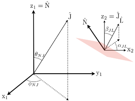
For the precessing binaries, LIGO-scale studies have been complicated by poor choice of coordinates, associated with the start of the waveform. The waveform generation code of the standard LIGO algorithm defines all the geometrical parameter values at the initial frequency (40 Hz for the initial LIGO and 10 Hz for the advanced LIGO), and evolve the binary system to get the full waveforms. Specifically, the orbit is described at some point, including the spin, orbital angular momentum vector, and the orbital phase. By contrast, the detector is more sensitive to higher frequencies. Allowing for the decreasing signal strength with frequency Bro12 , the detector is most sensitive to the instantaneous binary configuration at 100 Hz (initial LIGO) and 40 Hz (advanced LIGO, e.g., see Fig. 2 in Bro12 ). Motivated by this fact, we choose the reference frequency (), at which the instantaneous orientations of the spins and orbital plane are defined, to be 100 Hz.
One significant effect introduced by setting the reference frequency at 100 Hz is related to the orbital phase. The ambiguity function is dependent on how we choose the reference frequency. In appendix B, we describe an example and illustrate the significant effects in detail; see also Fig. 2.
Furthermore, following Brown et al.Bro12 , we define the geometrical parameters to be angles between the radiation vector , total angular momentum axis and orbital axis as in Fig. 1. For comparison, other conventions specify some parameters using the line of sight, a vector pointing from our detector to the binary.
For non-spinning or aligned-spin binaries, the total angular momentum is parallel to the orbital angular momentum and the orbital axis is fixed. In effect, the conventional radiation frame is equivalent to the geometrical frame.
II.3 Fiducial simulations and local coordinates
In the case of a non-spinning binary, the binary is specified by 9 parameters. In this work, we choose masses () as intrinsic parameters, the polar (inclination) and azimuthal (polarization) angles () of the orbital axis with respect to the radiation vector and an orbital phase as extrinsic parameters. Because we maximize the ambiguity function over the polarization, we need not take this parameter into explicit account henceforth. Remaining parameters are, the distance to the detector, sky position (two angles), and the coalescence time. The fiducial values of parameters are summarized in Table 1. Mass components () can be expressed by the symmetric mass ratio and chirp mass , we adopt these parameters in this work.
If the NS spin is assumed to be 0, the aligned-spin binary is specified by 10 parameters. 9 parameters are the same as the non-spinning case and the additional intrinsic parameter is dimensionless BH spin parameter . The fiducial values are also summarized in Table 1.
| parameter | |||||||
|---|---|---|---|---|---|---|---|
| non-spinning | 10 | 1.4 | 0.0 | 0.0 | 2.994 | 0.1077 | |
| aligned-spin | 10 | 1.4 | 0.0 | 1.0 | 2.994 | 0.1077 |
The waveform of the precessing binary can be defined by 12 parameters if the NS spin is assumed to be 0. In this work, we consider , , BH spin , and the opening angle of the precessing cone as intrinsic parameters, , , , and the orbital phase as extrinsic parameters. Because we maximize over the polarization angle , the parameter is eliminated from further consideration. Remaining parameters are the distance, sky position (two angles), the coalescence time. Throughout this paper the units are solar masses (for ); radians (for angles); or the natural dimensionless units (for ).
Motivated by Bro12 , we adopt a challenging reference configuration, where the polarization along the line of sight oscillates between circularly polarized ( along ) and linearly polarized ( perpendicular to ). Furthermore, to explore the extent to which higher-order harmonics allow measurement of parameters that only weakly impact the signal, we consider two possible sets of initial conditions for along its precession cone. The fiducial values of the parameters are summarized in Table 2. For case1, the orbital axis is perpendicular to the radiation vector at 100 Hz, for case2 it is parallel to the radiation vector at 100 Hz. All the parameter values are the same between both cases except for .
| parameter | configuration | |||||||
|---|---|---|---|---|---|---|---|---|
| case1 | 10 | 1.4 | 1.0 | 0.0 | 0.0 | |||
| case2 | 10 | 1.4 | 1.0 | 0.0 |
II.4 Fiducial network
We assume two identical interferometers placed perpendicular to the incident signal, which is the optimal sky position of the source. We also assume the two interferometers are oriented by related to one another, giving comparable sensitivity to both polarizations. For the incident waveforms, we assume a zero noise limit to understand how similar the signals are. While not realistic, they avoid introducing complexity of the signal due to the source sky position.
III distinguishing simulations
III.1 Ambiguity function
In this work, we reorganize the two projections of the strain tensor and into a complex function:
| (1) |
We coherently compare a fiducial signal , where indicates a fiducial source parameter set, to a nearby signal , with parameters , by a complex overlap Osh12
| (2) |
where is the Fourier transform of and is a detector strain noise power spectrum. For simplicity, we adopt a semianalytic initial LIGO sensitivity Dam01 ; Aji09 . As pointed out by Osh12 , this complex-valued expression characterizes the ability of a network to distinguish signals. The real part of the complex overlap corresponds to a linear sum of the conventional real overlaps of the two gravitational wave polarizations:
| (3) |
where indicates the conventional overlap of two real functions defined by
| (4) |
In appendix A, we summarize the differences between the real and complex overlaps.
We note that a change of the polarization angle, , simple causes a rotation of the argument of the complex wave strain function, . Thus it is trivial to find the value of which makes the complex overlap purely real, so that
| (5) | |||||
and the value of the complex overlap maximized over polarization angle is simply
| (6) |
The complex overlap (like the real-valued overlap) can also be maximized over the coalescence time via an inverse Fourier transform as described in All05 . In particular, one uses the fact that
| (7) |
and notes that the inverse Fourier transform of the complex overlap integrand in Eq. (2) will compute the complex overlap for all possible coalescence times of at once
| (8) |
The (normalized) ambiguity function between two waveforms and is then defined as the complex overlap maximized over polarization angle and coalescence time,
| (9) |
Unless otherwise noted, all overlaps are maximized in time and polarization. This is different from maximizing over orbital phase ; see appendix A and B.
III.2 Likelihood
The detector noise is assumed to be a stationary and Gaussian process. Given the detector output representing a real-valued signal in real-valued noise, the probability for the noise to have some realization is Fin92
| (10) |
The posterior probability that the gravitational wave signal is characterized by the parameters , can be expressed by , where is the prior probability that the signal is characterized by , is the likelihood, which can be written by Fin92
| (11) |
where is a proportional factor which, for simplicity, we assume to be 1 in this work.
Since we consider the complex strain, by choosing the appropriate polarization angle we shall write the detector output for the detector 1 and 2.
| (12) |
also
| (13) |
The probability for the noise to have both realizations and is
Finally, using Eqs. (12 - III.2), Eq. (11) can be expressed by the complex signals:
| (15) |
Substituting into this equation Cut07 , the likelihood is
where the second and third terms in the a square bracket depend on the noise realization. They shift the position of the maximum likelihood but only weakly change the shape of the likelihood curve. In the limit of high SNR, these noise-dependent terms can be neglected, so,
This equation corresponds to the case where two detectors are placed to have the maximum response to the incident two polarizations [for the detector placement, see Section II D]. While, Eq. (11) corresponds to one detector response to one polarization; see appendix A.
Using Eqs. (6) and (9), and the SNR defined by , the log likelihood can be expressed by our complex overlap convention:
| (18) |
where we assume the same strength for both signals.
For a given log likelihood, the scale of interest of the ambiguity function depends on the signal strength :
| (19) |
By approximately identifying the surface of the likelihood, this condition allows us to estimate the set of parameters which cannot be distinguished from with a signal amplitude of using a signal model and noise curve that produces an overlap .111More properly, the probability of having likelihood lets us create a confidence volume for any target confidence level. Because the probability depends sensitively on , we anticipate the edge of this confidence interval will depend weakly (e.g., as ) on the precise probability used to define the threshold.
III.3 Fisher matrix
If is close to , we can write to the first order in the error
| (20) |
So, in the limit of high SNR, the likelihood [Eq. (III.2)] is given as , where is
| (21) |
This definition is analogous to the standard Fisher matrix, except that it is derived from the complex overlap and therefore contains information about both polarizations. If we assume that the prior is uniform, the parameter estimation errors (i. e., the posterior probability density function) can be expressed by the Gaussian distribution
| (22) |
where is the corresponding normalization factor.
Using another expression relating the Fisher matrix to the log likelihood Jar94 ; Val08 and Eq. (18), we can write
where is the fiducial value of source parameter. Here, we define the normalized Fisher matrix .
For Gaussian noise and high SNR, the inverse of the Fisher matrix is the covariance matrix () of parameter errors. The measurement error () of each parameter and correlation coefficient () between two parameters are defined as
| (24) |
The correlation coefficients are -independent but often sensitive to small changes in . Conversely, the measurement error is inversely proportional to . For the purposes of illustration, we adopt whenever we calculate .
III.4 Relevant scales and effective approach
The Fisher matrix formally involves derivatives, i.e., infinitesimal variations of a parameter . In this work, we compute an effective Fisher matrix by considering finite variations on scales which give physically observable changes to the ambiguity function, .
To understand the variability on multiple scales we plot a one-dimensional ambiguity function of for the leading-order amplitude, non-spinning binary in Fig. 2. In this figure, the ambiguity function is calculated via Eq. (9), changing only and fixing all other parameters to be the same for both signals. For comparison, we plot quadratic fits222Since the posterior function is a normal distribution in the limit of high SNR (see Eq. (22)), a quadratic fitting function usually best fits the log likelihood function with a flat prior. to the ambiguity curve at different scales of and . These are the scales of interest for signals with strength or (see, Eq. (19)). [Note that Fig. 2 is computed with the reference frequency at 40 Hz. For our results, except for this figure, we choose the reference frequency at 100 Hz. The structure illustrated here is present but less significant at 100 Hz; see appendix B.]
The shape of the ambiguity function has structure on multiple scales. The neighborhood of suggests a much sharper peak than what is seen at the scale. A Fisher matrix computed from formal waveform parameter derivatives (defined in the limit ) or finite difference such that can be overly optimistic about how well can be measured for a signal with .
Therefore, we wish to define an effective Fisher matrix from the curvature of the ambiguity function on the scales of interest. For example, in the case of two parameters, the fitting function is
| (25) |
where and are fitting coefficients and . We calculate the effective Fisher matrix as
| (26) |
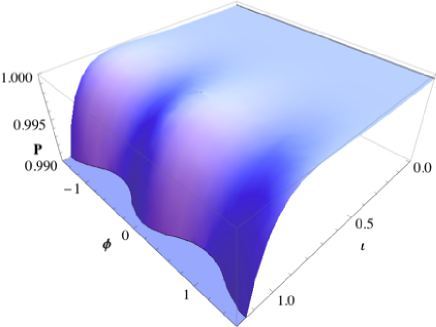
In some cases, especially when a parameter is poorly determined, the variation of the ambiguity function with a parameter may not be well-described by a quadratic. See, for example, the top panel of Fig. 5. Therefore, we find it useful to employ an “iterative” procedure to find the parameters that are amenable to a quadratic fit. For each parameter , we compute the one-dimensional curve and fit it against . This determines the diagonal elements of the effective Fisher matrix, . We discard any parameters that are poorly fit by this quadratic (checked either “by eye” or a with quantitative threshold on the goodness of fit). For the well-fit parameters, we determine the off-diagonal elements of the Fisher matrix by computing the two-dimensional surface and fitting it to a function of the form like Eq. (25) while using the values from the one-dimensional fits, i.e. . We note this method is used primarily as a sanity check to identify any parameters which induce obviously non-quadratic variations in .
Once we have identified the space of all reasonably quadratic parameters, the ambiguity function on that space can be approximated as
| (27) |
Rather than using the iterative procedure described above to find the elements of one at a time, it is straightforward to use a standard least-squares fitting technique to simultaneously solve for all of the . This will also give a better global approximation to the ambiguity function than the iterative approach. As an example of the small yet noticeable differences between these two procedures, Table 6 compares the results for computing the effective Fisher matrix from both “iterative” and “simultaneous” fits to the ambiguity function. Everywhere else in this work (Tables 3, 4, 5, 6, 7, and 9) the effective Fisher matrix is computed by simultaneously fitting all coefficients.
In the cases where is not well-described by a quadratic (e.g., see Fig. 5), we can adopt more complicated expressions to characterize the functional dependence of when these parameters are varied, both in isolation and in correlation with well-constrained variables. As a concrete example, in the absence of higher harmonics the line of sight from the binary is both weakly constrained by observations and nearly separable in from other degrees of freedom333Approximate separability of the line of sight from other degrees of freedom follows only in our well-chosen coordinates, where the binary configuration is specified at . . Specifically, ignoring maximization in time and phase, the overlap between any two lines of sight can be well-approximated by Eq. (B1c) from Osh12 :
where we use the shorthand and similarly for to reduce superfluous subscripts and where we factor out the common from . This function has wide, nearly flat extrema in for each fixed . On the other hand, in the absence of higher harmonics the line of sight has little impact on the waveform phase versus time away from the orbital plane. We can therefore approximate the ambiguity function for in the top panel of Fig. 5 by
| (29) |
where the index varies over the line-of-sight parameters and the indices vary over the other parameters and for . With higher harmonics, the functional form above [Eq. (29)] is weakly perturbed by additional angular terms of the form
| (30) | ||||
where is a matrix with . This approximation both factors out the leading-order angular dependence and adds additional angular terms with parameter-dependent coefficients, designed to correctly reproduce a -independent result when . Although these terms allow us to correctly reproduce the non-ellipsoidal contours seen in the bottom panel of Fig. 5, Tables 6 and 7 show that this complicated structure only marginally improves the overall fit compared to a purely quadratic approximation . Fit parameters for this more complicated functional dependence are not presented here.
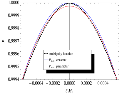
We also considered a more general fit, treating as a parameter. While this parameterization has a significant aesthetic advantage – its effective Fisher matrix is roughly scale-independent when and agrees with analytic calculations – it systematically underestimates in the neighborhood of the maximum. As both fits work well globally, we favor the simpler procedure and adopt except for Table 5.
III.5 Comparing to standard Fisher matrix results
Despite subtle differences associated with time domain versus frequency domain waveforms, the complex overlap, higher harmonics, and the line of sight, our results for the effective Fisher matrix are directly comparable to earlier results calculated with the stationary phase approximation Poi95 . For example, for emission along the axis, both the real and complex strain have the form444The two differ for : the complex strain has , while the real strain has . for . As a result, the Fisher matrix can be well-approximated by an identical average over frequency:
| (31) |
where we neglect derivatives as small compared to the leading-order phase dependence. Thus, each component of our Fisher matrix must resemble previous results. In fact, as the general definition [Eq. (21)] suggests, each component of (unlike ) depends only on the local response to changing two parameters , no matter how many parameters exist in the model. Therefore, the Fisher matrix for an identical model with more parameters will have, as a submatrix, the Fisher matrix for the smaller model. By contrast, other methods for expressing uncertainty like the covariance depend simultaneously on all terms in . For low-mass binaries, the Fisher matrix is well-known to be poorly conditioned, with eigenvalues spanning several orders of magnitude. We therefore preferentially compare the component-by-component Fisher matrix, rather than the covariances , when comparing results. When presenting results, we provide several significant figures to insure all eigenvalues of remain positive-definite.
Our complex overlap maximizes over time and polarization. The analytic Fisher matrix calculated from the stationary phase approximation [Eq. (31)] has time and phase as parameters. To account for maximizing over those parameters, we transform the full Fisher matrix to a smaller-dimensional matrix which projects out those dimensions:
| (32) | |||||
| (33) |
where run over the variables and all other variables. In these expressions, the matrix is the inverse of the projection of into the subspace.
III.6 Comparing to posteriors
Standard parameter estimation techniques like Markov-Chain Monte Carlo produce samples of the full posterior probability distributions, including postprocessed data products like one-dimensional standard deviations and two-dimensional covariances . For strong signals with well-isolated probability distributions, our one-dimensional standard deviations and covariances are directly comparable, for identical binaries. For fainter signals with broad probability distributions, our results will describe part of the posterior, in the neighborhood of one extremum.
For brevity, we have explicitly eliminated two parameters – event time and polarization – and make no predictions about any correlation including them. We will revisit these parameters, along with asymmetric detector response, in a subsequent publication.


III.7 Numerical and systematic effects
At the very smallest scales, delicate implementation-dependent choices can also introduce artificial structure into the ambiguity function. We have already extensively described how the choice of reference frequency introduces (coordinate-dependent) structure. Less physically, the sampling rate for the waveforms can produce artificial small-scale structure; to avoid this effect we sample at a variety of data rates, typically either (for ) or (for ). Finally, the ambiguity function can also be impacted by our choice for the starting and ending frequency. For our calculations, we start integrating the waveform and integrate over all power above . In our experience, this procedure best mimics the real data processing used in initial LIGO searches. However, a not-insignificant amount of power is present between and ; if included in the integral, the overlap would differ by , comparable to some fine-scale structures of interest. At the other extreme, we terminate our evolution at the minimum-energy circular orbit (MECO), where the binary energy ceases to decrease monotonically.
One small, subtle, but important effect is the nonzero overlap of the waveforms along the axis555Such waveforms would have a real overlap of unity, but the complex overlap is expected to be zero. See Appendix A.. For example, for our non-precessing binary, we find that for otherwise identical parameters
| (34) |
Equivalently, in the language of single-detector real overlaps, the sine and cosine chirps are not precisely orthogonal, for the same orbital phase666The real overlap is usually performed in conjunction with an explicit maximization over time and orbital phase, for a single harmonic. For that situation, this subtlety does not occur.. To a first approximation the signals are basis waveforms; the waveform along any line of sight is a superposition of the two. Because these two signals are not orthogonal, the ambiguity function generally has fine-scale structure with , associated with the overlap of these two directions. For example, on this scale and below, the overlap between two non-precessing waveforms with just emission is no longer well-described by Eq. (III.4). Instead, the ambiguity function gains additional fine-scale structure in angle. While extremely useful, for our purposes this result means that on sufficiently small scales , the complex overlap will have additional structure compared to “conventional” investigations of single-detector, optimally-oriented overlaps (i.e., overlaps of two real signals, extracted along ). In particular, this nonzero overlap is partially responsible for the small-scale structure seen in Fig. 3.
Because of the many subtle interpretation and implementation issues associated with the smallest ambiguity scales, while we investigate the value of effective fitting to fine scales (e.g., ), for simplicity we emphasize results for the scale relevant to most detection events ().
IV Results
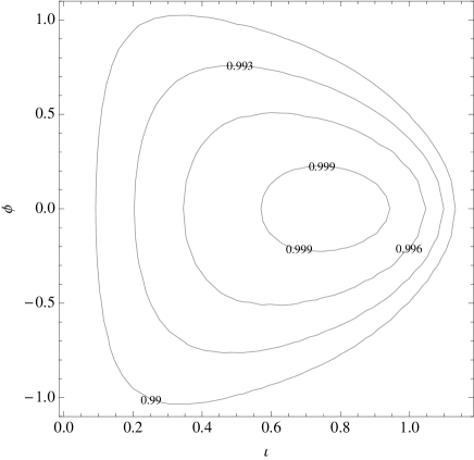
Using a small set of fiducial simulations, we compare non-precessing and precessing signals against their immediate neighbors, mapping out an ambiguity function in each -dimensional parameter space.
Higher harmonics perturb the ambiguity function by a quantifiable amount (i.e., for depending on and the harmonic). As has previously been shown elsewhere, we find that higher harmonics break degeneracies present in non-precessing, leading-order signals Bro07 ; Lan06 ; Por08 .
As described below, we generally find small but significant scale-dependent disagreement with the conventional stationary-phase Fisher matrix calculation, even in the absence of higher harmonics. Motivated by Figs. 2 and 3, as well as the Appendix and Figs. 10 and 11, we suspect that most scale dependence is introduced by suboptimal coordinates and can be minimized by a better choice of reference frequency. Despite our best attempts to find coordinates well-adapted to the problem, the change in going from to for leading-order waveforms is comparable to the change in going from leading-order waveforms to higher harmonics.
| pN order | leading-order | higher-order | |||||||||
|---|---|---|---|---|---|---|---|---|---|---|---|
| fitting scale | |||||||||||
| parameter | |||||||||||
| 3012 | -5505 | 3621 | -6474 | 2547 | -5314 | 3243 | -6070 | 3932 | -7224 | ||
| - | 10675 | - | 12478 | - | 11954 | - | 12151 | - | 14367 | ||
| 1.00 | 0.971 | 1.00 | 0.963 | 1.00 | 0.963 | 1.00 | 0.967 | 1.00 | 0.961 | ||
| - | 1.00 | - | 1.00 | - | 1.00 | - | 1.00 | - | 1.00 | ||
| 0.00760 | 0.00404 | 0.00618 | 0.00333 | 0.00735 | 0.00339 | 0.00689 | 0.00356 | 0.00578 | 0.00302 | ||
| fitting scale | |||||
|---|---|---|---|---|---|
| parameter | |||||
| 3883 | -7236 | -0.08350 | 0.08169 | ||
| - | 14209 | 0.1181 | 1.172 | ||
| - | - | 0.02723 | -0.001413 | ||
| - | - | - | 0.03196 | ||
| 1.00 | 0.976 | -0.00313 | -0.271 | ||
| - | 1.00 | -0.00494 | -0.276 | ||
| - | - | 1.00 | 0.0474 | ||
| - | - | - | 1.00 | ||
| 0.00740 | 0.00387 | 0.607 | 0.583 | ||
| pN order | leading-order | higher-order | |||||||||
|---|---|---|---|---|---|---|---|---|---|---|---|
| fitting scale | |||||||||||
| 0.999767 | 0.999884 | n/a | 0.999775 | 0.999888 | |||||||
| parameter | |||||||||||
| 2899 | -5295 | 2980 | -5325 | 2546 | -5313 | 3125 | -5848 | 3274 | -6014 | ||
| - | 10261 | - | 10276 | - | 11954 | - | 11701 | - | 11974 | ||
| 1.00 | 0.971 | 1.00 | 0.962 | 1.00 | 0.963 | 1.00 | 0.967 | 1.00 | 0.960 | ||
| - | 1.00 | - | 1.00 | - | 1.00 | - | 1.00 | - | 1.00 | ||
| 0.00776 | 0.00413 | 0.00673 | 0.00363 | 0.00735 | 0.00339 | 0.00704 | 0.00364 | 0.00628 | 0.00328 | ||
| pN order | leading-order | higher-order | ||||||||||||||
| method | iterative | simultaneous | iterative | simultaneous | ||||||||||||
| parameter | ||||||||||||||||
| 3686 | -1652 | -1007 | 3567 | -1570 | -975.6 | 2837 | -2423 | -669.6 | 4217 | -2147 | -1177 | 4129 | -2083 | -1157 | ||
| - | 1237 | 515.5 | - | 1170 | 492.4 | - | 2357 | 612.3 | - | 1806 | 685.6 | - | 1765 | 670.5 | ||
| - | - | 283.8 | - | - | 275.5 | - | - | 163.8 | - | - | 340.0 | - | - | 335.5 | ||
| 1.00 | -0.947 | 0.996 | 1.00 | -0.957 | 0.997 | 1.00 | -0.981 | 0.994 c | 1.00 | -0.929 | 0.994 | 1.00 | -0.935 | 0.995 | ||
| - | 1.00 | -0.969 | - | 1.00 | -0.974 | - | 1.00 | -0.995 | - | 1.00 | -0.958 | - | 1.00 | -0.962 | ||
| - | - | 1.00 | - | - | 1.00 | - | - | 1.00 | - | - | 1.00 | - | - | 1.00 | ||
| 0.0291 | 0.0180 | 0.135 | 0.0323 | 0.0201 | 0.149 | 0.0512 | 0.0621 | 0.440 | 0.0227 | 0.0131 | 0.104 | 0.0238 | 0.0137 | 0.108 | ||
| fitting scale | ||||||
|---|---|---|---|---|---|---|
| parameter | ||||||
| 4388 | -2256 | -1230 | -0.2527 | -0.5585 | ||
| - | 186928 | 719.09.8 | 0.30000.31 | 1.122 | ||
| - | - | 356.2 | 0.1098 | 0.3396 | ||
| - | - | - | 0.032790.0009 | -0.001972 | ||
| - | - | - | - | 0.02530 | ||
| 1.00 | -0.960 | 0.997 | -0.206 | -0.622 | ||
| - | 1.00 | -0.976 | 0.189 | 0.567 | ||
| - | - | 1.00 | -0.204 | -0.616 | ||
| - | - | - | 1.00 | 0.186 | ||
| - | - | - | - | 1.00 | ||
| 0.0324 | 0.0177 | 0.147 | 0.566 | 0.818 | ||
| pN order | leading-order | |||||||
|---|---|---|---|---|---|---|---|---|
| parameter | ||||||||
| 3234 | -281.1 | -612.8 | 868.8 | -1.359 | 3.726 | -10.18 | ||
| - | 929.9 | -3.089 | -171.7 | 1.252 | -6.253 | 11.33 | ||
| - | - | 132.0 | -177.3 | 0.3616 | -0.1832 | 2.147 | ||
| - | - | - | 295.2 | 0.06336 | 1.674 | -6.945 | ||
| - | - | - | - | 0.7774 | -0.003074 | 0.006970 | ||
| - | - | - | - | - | 0.3349 | -0.1021 | ||
| - | - | - | - | - | - | 0.3829 | ||
| 1.00 | 0.407 | 0.730 | 0.144 | -0.0729 | -0.109 | - | ||
| - | 1.00 | 0.742 | 0.729 | -0.183 | 0.109 | - | ||
| - | - | 1.00 | 0.752 | -0.180 | -0.133 | - | ||
| - | - | - | 1.00 | -0.191 | -0.106 | - | ||
| - | - | - | - | 1.00 | 0.0126 | - | ||
| - | - | - | - | - | 1.00 | - | ||
| 0.00592 | 0.00573 | 0.0433 | 0.0212 | 0.116 | 0.187 | - | ||
| pN order | higher-order | |||||||
| parameter | ||||||||
| 3401 | -408.2 | -644.3 | 911.9 | -1.745 | 4.515 | -11.89 | ||
| - | 1055 | 7.249 | -208.3 | 1.495 | -7.229 | 12.58 | ||
| - | - | 139.3 | -186.3 | 0.5298 | -0.1706 | 2.471 | ||
| - | - | - | 307.9 | 0.02350 | 1.998 | -7.544 | ||
| - | - | - | - | 0.8305 | 0.003262 | 0.006150 | ||
| - | - | - | - | - | 0.3510 | -0.1029 | ||
| - | - | - | - | - | - | 0.3951 | ||
| 1.00 | 0.543 | 0.778 | 0.309 | -0.154 | -0.177 | - | ||
| - | 1.00 | 0.815 | 0.786 | -0.265 | -0.00409 | - | ||
| - | - | 1.00 | 0.815 | -0.270 | -0.230 | - | ||
| - | - | - | 1.00 | -0.271 | -0.204 | - | ||
| - | - | - | - | 1.00 | 0.0381 | - | ||
| - | - | - | - | - | 1.00 | - | ||
| 0.00626 | 0.00626 | 0.0495 | 0.0237 | 0.115 | 0.188 | - | ||
| pN order | leading-order | |||||||
|---|---|---|---|---|---|---|---|---|
| parameter | ||||||||
| 3279 | -291.4 | -618.8 | 878.7 | -2.168 | 3.982 | -11.58 | ||
| - | 922.8 | -5.187 | -175.5 | 1.648 | -6.132 | 11.80 | ||
| - | - | 132.3 | -177.9 | 0.4429 | -0.2340 | 2.321 | ||
| - | - | - | 295.1 | 0.1488 | 1.674 | -7.263 | ||
| - | - | - | - | 0.8038 | -0.004911 | 0.005865 | ||
| - | - | - | - | - | 0.3299 | -0.1100 | ||
| - | - | - | - | - | - | 0.3850 | ||
| 1.00 | 0.477 | 0.747 | 0.238 | -0.0961 | -0.104 | - | ||
| - | 1.00 | 0.807 | 0.792 | -0.265 | 0.0961 | - | ||
| - | - | 1.00 | 0.801 | -0.251 | -0.108 | - | ||
| - | - | - | 1.00 | -0.284 | -0.0817 | - | ||
| - | - | - | - | 1.00 | 0.0119 | - | ||
| - | - | - | - | - | 1.00 | - | ||
| 0.00622 | 0.00661 | 0.0495 | 0.0241 | 0.117 | 0.187 | - | ||
| pN order | higher-order | |||||||
| parameter | ||||||||
| 3403 | -420.2 21 | -640.4 | 916.4 | -2.845 | 5.016 | -12.35 | ||
| - | 1057 | 18.55 | -212.3 | 1.533 | -7.488 | 12.73 | ||
| - | - | 137.2 | -185.2 | 0.6655 | -0.2104 | 2.472 | ||
| - | - | - | 308.5 | -0.01406 | 2.022 | -7.594 | ||
| - | - | - | - | 0.8481 | 0.003203 | 0.01161 | ||
| - | - | - | - | - | 0.3456 | -0.1035 | ||
| - | - | - | - | - | - | 0.3911 | ||
| 1.0 | 0.391 | 0.726 | 0.127 | -0.0705 | -0.193 | - | ||
| - | 1.00 | 0.718 | 0.712 | -0.226 | 0.0670 | - | ||
| - | - | 1.00 | 0.744 | -0.224 | -0.234 | - | ||
| - | - | - | 1.00 | -0.252 | -0.170 | - | ||
| - | - | - | - | 1.00 | 0.0224 | - | ||
| - | - | - | - | - | 1.00 | - | ||
| 0.00584 | 0.00529 | 0.0421 | 0.0210 | 0.113 | 0.191 | - | ||
IV.1 Zero spin
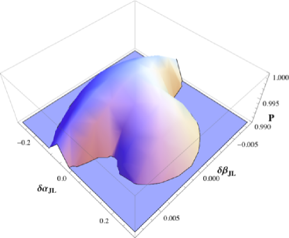
For a system without spin, higher harmonics principally provide information about the line of sight. For clarity, we will first discuss the most immediately relevant scale (). Comparing the solid (without higher harmonics) and dotted (with higher harmonics) curves on the top panel of Fig. 4, we immediately see that higher harmonics provide little new information about intrinsic parameters, all other things being equal. Equivalently, looking at Table 3, the effective Fisher matrix on the two-dimensional parameters without and with higher harmonics are similar to each other, as well as to a standard Fisher matrix computed using stationary phase approximation waveforms (labeled as ). By contrast, as illustrated by the dramatic difference between the top and bottom panel in Fig. 5, higher harmonics produce a dramatic qualitative change in how well the line of sight can be measured.
Both with and without higher harmonics [Fig. 5], the line of sight is very difficult to measure, particularly at the expected relevant scale (i.e., SNR of around ). In both cases, the ambiguity function has a broad, extended, asymmetric extremum. In the absence of higher harmonics, the ambiguity function cannot be usefully described by a locally quadratic approximation, even a effective one. Nonetheless, by understanding the expected dependence on angle (and by adopting coordinates in band), we can propose a physically-well-motivated fitting function, both for the purely angular dependence and for the correlations between line of sight and other parameters [Eq. (30)]. This fitting function works extremely well when higher harmonics are neglected. When higher harmonics are included, a quadratic approximation sufficies, as the local extremum is much narrower. In the latter case, Table 4 provides the fitting parameters needed to reconstruct the full multidimensional fit. In fact, our well-chosen reference frequency produces a nearly separable fit, with zero off-diagonal terms [e.g., in Eq. (30)]. We will return to this simple structure frequently below.
Several effects besides higher harmonics also introduce fine-scale structure into the ambiguity function. As demonstrated in Fig. 2, the choice of reference frequency can introduce strong, scale-dependent features into the ambiguity function. We chose a reference frequency at to reduce its effect, but have not eliminated it completely. The nonzero overlap between the modes is another such effect. Hence, we are not surprised that our effective fitting parameters change as we reduce the range of used in the fit, even in the absence of harmonics; see Table 3.
The effect of scale dependence is fairly mild: the eigendirections for and agree, only the eigenvalue scale changes. For comparison, we also considered an alternate fitting technique that allowed the single best fit point to have ; see Fig. 3, and Table 5. While this method leads to aesthetically pleasing results similar to analytic calculations, this fit systematically underestimates near the maximum-likelihood point and does not completely eliminate the trend towards different fitting parameters on the smallest scales. We henceforth adopt .
To facilitate approximate comparisons with prior work, Tables 3 and 4 provide one-dimensional standard deviations and correlation coefficients . Unless otherwise stated, these quantities are derived solely from the Fisher matrix fits from that same table. For example, in Table 3, the “measurement errors” follow from inverting the matrix shown, while in Table 4 they follow from inverting a full matrix.
IV.2 Aligned spin
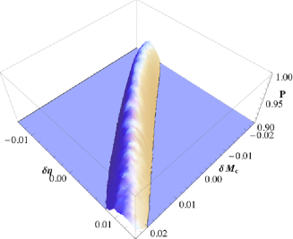
Repeating our effective Fisher matrix calculation for an aligned-spin BH-NS binary leads to results qualitatively similar to the zero-spin case. As previously, higher harmonics provide little additional information about intrinsic parameters, here ; see Fig. 6. For example, looking at data along a fixed line of sight, Table 6 shows that, on a component-by-component basis () and overall (), the two ambiguity functions with and without higher harmonics resemble one another. More directly, Fig. 6 shows three-dimensional contours of nearly constant as a function of for both leading-order emission (blue) and higher harmonics (red). While higher harmonics clearly do provide more information about intrinsic parameters – the red surface is nested inside the blue – the addition of higher harmonics only marginally improves our ability to measure the least-well-constrained combination of . Precisely as in the non-spinning case, however, higher harmonics provide more information about the line of sight. Despite our line of sight providing some sensitivity to a symmetry-breaking harmonic, a waveform with harmonics encodes roughly similar information as a waveform without harmonics. Tables 6 and 7 provide the effective fitting parameters we used to reproduce their ambiguity function. As in the non-spinning case, we find an approximately separable fit, though less so than before [see in Table 7]. Even allowing for weak correlations between intrinsic parameters and the line of sight, the overall parameter covariances with harmonics [Table 7] are nearly unchanged from a model with only leading-order emission [Table 6].777For leading-order emission, measurements of orientation and intrinsic parameters separate completely. The intrinsic parameter uncertainties computed in Table 6 are therefore identical to the uncertainties for the corresponding parameters derived from a full Fisher matrix.
The aligned-spin results at cannot be easily compared with the corresponding zero-spin results (). On the one hand, the component-by-component Fisher matrix coefficients like will differ significantly, as the waveform phasing changes as a function of and hence so does . On the other hand, the aligned-spin results allow a new parameter (spin) that was treated as fixed for the case, with nontrivial coupling to the other intrinsic parameters. The one-parameter uncertainties are dramatically increased by including this previously-neglected systematic effect.
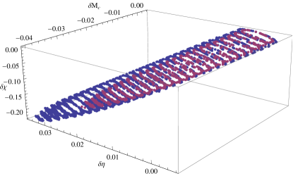
Both at leading and higher-order, our effective fit to the ambiguity function is complicated by the wide range of scales in , even for fixed line of sight. As is well-known from previous Fisher matrix calculations with aligned-spins Poi95 ; Cut94 , the ambiguity function in has strong correlations, producing a narrow and extended extremum. For the specific example described by our effective Fisher matrix, the submatrix has eigenvalues , describing a strong hierarchy of scales. For our purposes, Fig. 6 demonstrates our fiducial aligned-spin binary cannot be distinguished from binaries with spin : for each in this range, suitable combinations of exist with high overlap. For these extremely extended ambiguity ellipsoids, a fit that reproduces over the full range in might require a more generic functional form than the one adopted so far: a quadratic with constant coefficients in the neighborhood of the fiducial binary. Effectively speaking, however, these additional degrees of freedom add little information with considerable expense. We will explore more complicated effective dependence in a subsequent publication.
As in the zero-spin case, we find significant differences on the smallest scales in , in a fashion that depends on the reference frequency. Given the number of dimensions, complex functional form, sensitivity to numerical implementation like the sampling rate, and less immediate observational relevance, we defer a detailed discussion of fine-scale effects to a subsequent paper.
IV.3 Precessing spin: Case 1
For the first of our two fiducial precessing binaries, we find higher harmonics provide little added information beyond the constraints produced in the non-precessing case. This unfortunate but expected result can be seen, for example, from the one-dimensional covariances in Table 9; from the effective Fisher matrix coefficients ; or from their comparable sequences of eigenvalues. That said, even in the absence of higher harmonics, the ambiguity function for a precessing binary has simpler structure than the non-precessing result, with reduced correlations among the “intrinsic” parameters; a somewhat less extreme hierarchy of scales (i.e., eigenvalues)888We can always rescale our eigenvalues by rescaling our coordinate units. However, in these units all parameters have a prior range of order unity, and physical meaning. As a result, our eigenvalues also have meaning: the coordinate combinations corresponding to the smallest eigenvalues have minimal impact on the overlap and can be ignored.; and roughly speaking a more quadratic ambiguity function.
In fact, for a precessing binary the previous clear separation between “intrinsic” and “geometric” parameters breaks down. As each instant the opening angle of the precession cone of around depends on the relative magnitude of and , as well as on their (nearly conserved) misalignment angle . The magnitudes of and are essentially intrinsic parameters, characterizing the binary masses and BH spin; therefore, we expect the precession cone opening angle to be intimately correlated with the intrinsic parameters. At the same time, the precession cone opening angle must be intimately connected to the “geometric” parameters that define the orientation of the binary at the reference frequency: . Specifically, the orientation of the precession of relative to the line of sight is characterized by the two angles (setting the orientation of )999The other angle needed to specify the orientation of is equivalent to a rotation around the line of sight, i.e. the polarization angle. As the complex overlap maximizes over this angle, it is explicitly removed as a parameter. and (fixing the orientation of along the precession cone at the reference frequency). The orbital phase at the reference frequency fixes the binary’s geometry in band. This cross-coupling between intrinsic and extrinsic parameters has quantitative consequences for the Fisher matrix. Roughly speaking, the two new eigenvalues introduced into by allowing precession (here with values , associated with the and parameters) can be expected to lie between the very large () and very small () eigenvalues associated with the manifestly intrinsic () and extrinsic () parameters.
For non-precessing binaries, the choice of a Hz reference frequency nearly separated intrinsic and extrinsic parameters. A suitable choice of reference frequency may yet further reduce the off-diagonal terms in our effective Fisher matrix. For the present coordinates, however, we cannot cleanly decompose parameters into “intrinsic” and “geometric” parameters. Table 9 shows correlation coefficients calculated by omitting the (nearly unmeasurable) coordiante in ; no obvious block-diagonal form occurs.
IV.4 Precessing spin: Case 2
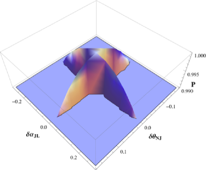
By contrast to the relatively simple ambiguity functions seen so far, our second set of binary parameters produces a significantly more complicated ambiguity function, particularly in geometric parameters. For example, Fig. 7 shows the ambiguity function versus and all other parameters fixed, for “case 2”. As in case 1, we have a highly symmetric binary starting with , and the line of sight in the same plane at our reference frequency. However, in this case we start with parallel to the line of sight, rather than perpendicular to it. The ambiguity function shows extreme sensitivity to the initial conditions and highly nonquadratic behavior. These differences occur despite the considerable similarity between case 1 and case 2: the two are, to an excellent approximation, the same configurations, just slightly offset in time. By contrast, the change in ambiguity versus is well-described by a quadratic form.
This extreme scenario demonstrates that even an effective Fisher matrix has limits: sometimes, a more generic functional form including higher-order correlations must be used on relevant scales. That said, highly nonquadratic behavior only occurred for a high-symmetry binary. We expect typical binary initial conditions will produce nearly quadratic ambiguity functions.
V Conclusions
In this paper we have used case studies of a coherent, two-detector ambiguity function to estimate how much and what kind of information higher harmonics provide about BH-NS binaries. Given the high dimension of and severe degeneracies that plague the problem, we perform a tractable, idealized calculation instead of the straightforward but less easily understood explicit source in a real multi-detector network. Specifically, we place a single source directly overhead an idealized detector pair, equally sensitive to both polarizations. For all binaries, we find that higher harmonics provide little additional information about the binary’s intrinsic parameters. Instead, at best they provide information about the orientation of the source relative to the line of sight (e.g., for non-precessing binaries). Notably, higher harmonics make it easier to exclude a non-precessing binary with .
When possible, we estimate the two-point function on scales of interest () by a locally quadratic function , whose coefficients we denote the “effective Fisher matrix.” Using coordinates adapted to the most sensitive frequencies of our network, we show that to an excellent approximation the Fisher matrix for non-precessing binaries separates into intrinsic (masses and spins) and extrinsic (geometric) parameters. For precessing binaries, the angles describing the precession cone are intimately connected with the intrinsic masses and spins as well as the geometric parameters. Therefore, they correlate with both intrinsic and extrinsic parameters and entangle the two previously distinct sets of parameters. In future work we will compare our results to detailed posterior parameter distributions, as computed by Markov-chain Monte Carlo simulations. Our results suggest suitable coordinates will substantially simplify the interpretation of these posteriors.
In addition to our main results, this paper also provides technical suggestions of broad interest to the data analysis community. First, rather than performing the conventional (single-polarization, real) overlap maximized over time and orbital phase, we use a coherent two-polarization overlap maximized over time and polarization Osh11 . This overlap is far more discriminating than the single-polarization result and, lacking a maximum over the polar emission direction , is well adapted to asymmetric situations such as precession or the presence of higher harmonics. Second, we illustrate the importance of choosing coordinates adapted to the network’s sensitive band and to the binary’s in-band geometry. We have provided concrete examples of the consequences of poor choices for coordinate conventions, which can lead to pathological behavior in the complex overlap and ambiguity function. Finally, we recommend adopting an effective Fisher matrix, derived by fitting the ambiguity function on the scale at which variations in the parameters could be plausibly detected. We have shown that the conventional approach to the Fisher matrix can be sensitive to unobservable fine-scale structure which can give misleading results. By contrast, simply by computing the ambiguity function over the area of interest, then fitting, one can explicitly verify whether a quadratic approximation even applies, as well as assess its error.
Acknowledgements
HSC, CK and CHL are supported in part by National Research Foundation Grant funded by the Korean Government (NRF-2011-220-C00029) and the Global Science experimental Data hub Center (GSDC) at KISTI. HSC and CHL are supported in part by the BAERI Nuclear R & D program (M20808740002) of MEST/KOSEF. CK is also supported by the Research Corporation for Scientific Advancement and by a WVEPSCoR Research Challenge Grant. ROS is supported by NSF award PHY-0970074, the Bradley Program Fellowship, and the UWM Research Growth Initiative. EO is supported by NSF award PHY-0970074.
Appendix A Comparison between the Real and Complex overlaps
One detector can not be sensitive to both polarizations, as it measures a single (real) strain variable . The conventional definition of the overlap [Eq. (4)] therefore provides an inner product for a single real data sequence.
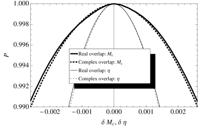
The complex overlap [Eq. (2)], however, uses information about both polarizations Osh12 . To illustrate the differences between these two diagnostics, Figs. 8 and 9 show the overlaps between our fiducial non-spinning waveform and an identical binary, except for one parameter. In both cases, these overlaps are maximized over event time and polarization (for the complex overlap) or orbital phase (for the real overlap).
First and foremost, Fig. 8 shows that the real overlap does not change as inclination () or the orbital phase () are varied. In other words, with one detector, we cannot identify the inclination, which measures the relative amplitude of to . Also, by maximizing over , we lose information about it. The conventional single-detector overlap therefore provides no information about how well we can measure these parameters in a network sensitive to two polarizations.
By contrast, because the complex overlap explicitly uses two polarizations, it can identify the inclination; see the dotted line in Fig. 8. For example, because it can distinguish between left- and right-handed sources, the overlap between antipodal directions (i.e., ) is zero. Moreover, if the source orientation is different from , then the waveform carries information about the orbital phase, which the complex overlap easily identifies. As a concrete example, if for the fiducial signal, the orbital phase is measurable at high SNR. When , is unmeasurable for the leading-order waveforms (for the analytic formula, see Eq. (B1) in Osh12 ) but marginally measurable for the higher-order waveforms (see Fig. 5).
On the other hand, when intrinsic parameters are varied, the complex and real overlaps largely agree, even though the complex overlap has more information available; see Fig. 9.
For the figures and discussion in this paper, we compare the real and complex normalized overlaps, dividing each network response by the network signal to noise. For the two identical detectors used in the complex overlap, the network SNR is just a quadrature sum of two detecters; see Eq. (3),
| (35) |
By contrast, for the real overlap, the relevant SNR is just . For an identical source, a two-detector network has higher overall SNR.
One point of this paper is to compare the real and complex overlaps from a parameter estimation point of view. Starting from Eq. (11), the real overlap enters directly into the expression for the posterior. As a result, contours of the real ambiguity function should closely correspond to contours of the posterior parameter distribution, for measurements limited to a single polarization and known sky location. By contrast, for a source with known sky location seen by a network with comparable sensitivity to both polarizations, the complex overlap enters directly into the expression for the posterior. A real network will have unequal sensitivity to two polarizations. We therefore expect the real posterior will resemble some average between the posteriors estimated using the single-detector and network overlaps. In a subsequent publication we will compare our results with posteriors computed by MCMC, to quantify how well our simple estimates do at characterizing measurement accuracy.

Appendix B Reference frequency and fine-scale structure in the ambiguity function and systematic errors
Even for a zero-spin binary with only leading-order harmonics, the choice of reference frequency at which the parameters are defined significantly influences the structure of the ambiguity function . As concrete examples, Figs. 9, and 11 show that specifying the orbital phase at the start or end of the waveform introduces additional structure on physical scales into the ambiguity function for the most well- determined and physical parameters, the chirp mass and mass ratio . Even more troubling, Fig. 10 shows that an ill-chosen reference frequency can introduce extremely fine-scale structure into the ambiguity function, for orientations away from . By contrast, a reference frequency close to the half-power point of the detector reduces these effects, where is estimated by
| (36) | |||||
| (37) |
for the standard restricted amplitude.
What introduces this severe dependence for such a vanilla waveform? The significant accumulation of orbital and hence waveform phase between the coordinates’ base point and the detector’s sensitive band. Roughly speaking, the detector is sensitive to the configuration of the binary as it crosses through its sensitive band. This trajectory can be characterized by some instantaneous parameters . By contrast, the waveform at a significantly earlier or later time has rotated roughly times between that frequency and the observed one. As a result, derivatives of the waveform relative to differ from derivatives relative to by a term of order . As a result, the more sensitive the waveform is to a parameter, the more severe the absolute impact of adopting a poor reference frequency.


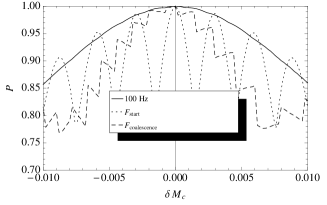
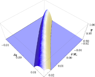
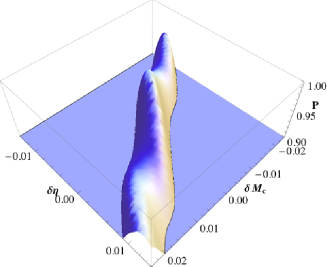
While we have chosen a single reference frequency, we have not optimized it, as we anticipate no single choice will work well for all parameters. The early part of the inspiral carries far more information about the chirp mass and mass ratio, as these both impact the total number of cycles. For example, to leading-order where the average corresponds to averaging in signal power (i.e., averaging over a distribution ). Evaluating the derivative and writing as an integral over frequency, we see the corresponding integrand to in the definition of is weighted by a polynomial in that is heavily biased towards low frequencies:
| (38) |
By contrast, spin effects enter at past leading-order in phase, suggesting the spin-spin Fisher matrix components are less severely biased towards low frequency;
| (39) |
Other components of the Fisher matrix arise from other averages over frequency and have other break-even points. In other words, for each measurable quantity, a generally distinct epoch of the signal provides the most information. No one breakeven point works for all.
References
- (1) Abbott et al. (The LIGO Scientific Collaboration). Nuclear Instruments and Methods in Physics Research A, 517, 154 (2004).
- (2) http://www.virgo.infn.it
- (3) Abbott et al. (The LIGO Scientific Collaboration). Phys. Rev. D 77, 062002 (2008).
- (4) Abbott et al. (The LIGO Scientific Collaboration). Phys. Rev. D 79, 122001 (2009).
- (5) A. Buonanno, Y. Chen, and M. Vallisneri, Phys. Rev. D 67, 104025 (2003).
- (6) A. Buonanno, Y. Chen, Y. Pan, and M. Vallisneri, Phys. Rev. D 70, 104003 (2004).
- (7) T. Damour, A. Gopakumar, and B. R. Iyer, Phys. Rev. D 70, 064028 (2004).
- (8) Y. Pan, A. Buonanno, Y. Chen, and M. Vallisneri, Phys. Rev. D 69, 104017 (2004).
- (9) C. Königsdörffer and A. Gopakumar, Phys. Rev. D 71, 024039 (2005).
- (10) A. Buonanno, Y. Chen, Y. Pan, H. Tagoshi, and M. Vallisneri, Phys. Rev. D 72, 084027 (2005).
- (11) C. Königsdörffer and A. Gopakumar, Phys. Rev. D 73, 124012 (2006).
- (12) M. Tessmer and A. Gopakumar, MNRAS, 374, 721 (2007).
- (13) M. Hannam, S. Husa, B. Brügmann, and A. Gopakumar, Phys. Rev. D 78 (2008)
- (14) I. Hinder, F. Herrmann, P. Laguna, and D. Shoemaker, arXiv:0806.1037.
- (15) K. G. Arun, A. Buonanno, G. Faye, and E. Ochsner, Phys. Rev. D 79, 104023 (2009).
- (16) A. Buonanno, B. R. Iyer, E. Ochsner, Y. Pan, and B. S. Sathyaprakash, Phys. Rev. D 80, 084043 (2009).
- (17) F. D. Ryan, Phys. Rev. D 52, R3195 (1995).
- (18) P. Jaranowski and A. Królak, Living Rev. Relativity 15, 4 (2012).
- (19) E. K. Porter and N. J. Cornish, Phys. Rev. D 78, 064005 (2008).
- (20) K. G. Arun, B. R. Iyer, B. S. Sathyaprakash, and S. Sinha, Phys. Rev. D 75, 124002 (2007).
- (21) C. Van den Broeck and A. S. Sengupta, Class. Quantum Grav. 24, 1089 (2007).
- (22) J. S. Key and N. J. Kornish, arXiv:1006.3759
- (23) R. N. Lang and S. A. Hughes, Phys. Rev. D 74, 122001 (2006).
- (24) A. Klein, P. Jetzer, and M. Sereno, Phys. Rev. D 80, 064027 (2009).
- (25) R. N. Lang, S. A. Hughes, and N. J. Cornish, Phys. Rev. D 84, 022002 (2011).
- (26) M. Vallisneri, Phys. Rev. D 77, 042001 (2008).
- (27) S. Vitale and M. Zanolin, Phys. Rev. D 82, 124065 (2010).
- (28) M. Vallisneri, Physical Review Letters 107, 191104 (2011).
- (29) L. Kidder, Phys. Rev. D 52, 821-847 (1995).
- (30) C. M. Will and A. G. Wiseman, Phys. Rev. D 54, 4813 (1996).
-
(31)
https://www.lsc-group.phys.uwm.edu/daswg/projects
/lal/nightly/docs/html/ - (32) D. A. Brown, A. Lundgren, and R. O’Shaughnessy, arXiv:1203.6060v2
- (33) R. O’Shaughnessy, J. Healy, L. London, Z. Meeks, and D. Shoemaker, arXiv:1201.2113v1
- (34) T. Damour, B. R. Iyer, and B. S. Sathyaprakash, Phys. Rev. D 63, 044023 (2001).
- (35) P. Ajith and S. Bose, Phys. Rev. D 79, 084032 (2009).
- (36) B. Allen, W. G. Anderson, P. R. Brady, D. A. Brown and J. D. E. Creighton, arXiv:gr-qc/0509116
- (37) L. S. Finn, Phys. Rev. D 46, 5236 (1992).
- (38) C. Cutler and M. Vallisneri, Phys. Rev. D 76, 104018 (2007).
- (39) P. Jaranowski and A. Królak, Phys. Rev. D 49, 1723 (1994).
- (40) E. Poisson and C. M. Will, Phys. Rev. D 52, 848 (1995).
- (41) C. Cutler and E. É. Flanagan, Phys. Rev. D 49, 2658 (1994).
- (42) R. O’Shaughnessy, B. Vaushnav, J. Hearly, Z. Meeks, and D. Shoemaker, Phys. Rev. D 84, 124002 (2011).