Minimal Radiative Neutrino Mass Mechanism for Inverse Seesaw Models

P. S. Bhupal Dev and Apostolos Pilaftsis
Consortium for Fundamental Physics, School of Physics and Astronomy, University of Manchester, Manchester, M13 9PL, United Kingdom.
Abstract

ABSTRACT

We study a minimal one-loop radiative mechanism for generating small Majorana neutrino masses in inverse seesaw extensions of the Standard Model with two singlet fermions per family. The new feature of this radiative mechanism is that the one-loop induced left-handed neutrino mass matrix is directly proportional to the Majorana mass matrix of the right-handed neutrinos. This is a very economical scenario without necessitating the existence of non-standard scalar or gauge fields.

preprint: MAN/HEP/2012/14

I Introduction

The understanding of the extra-ordinary smallness of neutrino masses, along with their observed large mixings vureview remains one of the major puzzles in the Standard Model (SM), and so a potential portal to New Physics. The simplest theoretical scenario which may explain this neutrino puzzle would be to introduce singlet Majorana masses that break the global (BL)𝐵𝐿(B-L)-symmetry of the SM. Within the SM, this can be parameterized through the non-renormalizable dimension-5 operator due to Weinberg weinberg : λij(Li𝖳Φ)(Lj𝖳Φ)/Λsubscript𝜆𝑖𝑗subscriptsuperscript𝐿𝖳𝑖Φsuperscriptsubscript𝐿𝑗𝖳ΦΛ\lambda_{ij}\,\left(L^{\sf T}_{i}\Phi\right)\left(L_{j}^{\sf T}\Phi\right)/\Lambda, where Li=(νi,i)L𝖳subscript𝐿𝑖superscriptsubscriptsubscript𝜈𝑖subscript𝑖𝐿𝖳L_{i}=(\nu_{i},\ell_{i})_{L}^{\sf T} (with i=e,μ,τ𝑖𝑒𝜇𝜏i=e,\mu,\tau) is the SU(2)L lepton doublet, Φ=(ϕ+,ϕ0)𝖳Φsuperscriptsuperscriptitalic-ϕsuperscriptitalic-ϕ0𝖳\Phi=(\phi^{+},\phi^{0})^{\sf T} is the SM Higgs doublet, and ΛΛ\Lambda is an effective mass scale of the New Physics. After electroweak symmetry breaking via the vacuum expectation value (VEV) of the Higgs field, Φ=(0,v)𝖳delimited-⟨⟩Φsuperscript0𝑣𝖳\langle\Phi\rangle=(0,v)^{\sf T}, the SU(2)L-doublet neutrinos νiLsubscript𝜈𝑖𝐿\nu_{iL} receive a non-zero mass matrix of the form (MνL)ij=λijv2/Λsubscriptsubscript𝑀subscript𝜈𝐿𝑖𝑗subscript𝜆𝑖𝑗superscript𝑣2Λ(M_{\nu_{L}})_{ij}=\lambda_{ij}v^{2}/\Lambda.

There exist three tree-level realizations type1 ; type2 ; type3 of this effective dimension-5 operator using only renormalizable interactions. The simplest one, widely known as the type-I seesaw type1 , requires the extension of the SM by a number nRsubscript𝑛𝑅n_{R} singlet fermions, which are usually taken to be heavy right-handed (RH) neutrinos ναRsubscript𝜈𝛼𝑅\nu_{\alpha R} (with α=1,2,,nR𝛼12subscript𝑛𝑅\alpha=1,2,\dots,n_{R}). After integrating out the heavy singlet neutrinos ναRsubscript𝜈𝛼𝑅\nu_{\alpha R}, we obtain Weinberg’s effective dimension-5 operator mentioned above. Specifically, the neutrino masses and mixings may be deduced from the Yukawa Lagrangian:

Y=(yν)iαL¯iΦναR+12ν¯αRC(MR)αβνβR+H.c.,formulae-sequencesubscript𝑌subscriptsubscript𝑦𝜈𝑖𝛼subscript¯𝐿𝑖Φsubscript𝜈𝛼𝑅12superscriptsubscript¯𝜈𝛼𝑅𝐶subscriptsubscript𝑀𝑅𝛼𝛽subscript𝜈𝛽𝑅Hc-{\cal L}_{Y}\ =\ (y_{\nu})_{i\alpha}\,\bar{L}_{i}\Phi\,\nu_{\alpha R}\>+\>\frac{1}{2}\bar{\nu}_{\alpha R}^{C}(M_{R})_{\alpha\beta}\nu_{\beta R}\ +\ {\rm H.c.}~{}, (1)

which in turn implies the following (3+nR)×(3+nR)3subscript𝑛𝑅3subscript𝑛𝑅(3+n_{R})\times(3+n_{R}) complex symmetric matrix in the flavor basis {(νiL)C,ναR}superscriptsubscript𝜈𝑖𝐿𝐶subscript𝜈𝛼𝑅\{(\nu_{iL})^{C},\nu_{\alpha R}\}:

ν=(𝟎MDMD𝖳MR),subscript𝜈0subscript𝑀𝐷superscriptsubscript𝑀𝐷𝖳subscript𝑀𝑅\displaystyle{\cal M}_{\nu}\ =\ \left(\begin{array}[]{cc}{\bf 0}&M_{D}\\ M_{D}^{\sf T}&M_{R}\end{array}\right)\;, (4)

where MD=yνvsubscript𝑀𝐷subscript𝑦𝜈𝑣M_{D}=y_{\nu}v is the Dirac mass matrix for the neutrinos and MRsubscript𝑀𝑅M_{R} is the (BL)𝐵𝐿(B-L)-breaking Majorana mass matrix of the RH neutrinos. In the usual seesaw approximation (MD)iα/(MR)αβ1much-less-thansubscriptsubscript𝑀𝐷𝑖𝛼subscriptsubscript𝑀𝑅𝛼𝛽1(M_{D})_{i\alpha}/(M_{R})_{\alpha\beta}\ll 1, the physical light neutrino masses are given by

MνLMDMR1MD𝖳.similar-to-or-equalssubscript𝑀subscript𝜈𝐿subscript𝑀𝐷superscriptsubscript𝑀𝑅1superscriptsubscript𝑀𝐷𝖳\displaystyle M_{\nu_{L}}\ \simeq\ -\,M_{D}M_{R}^{-1}M_{D}^{\sf T}\;. (5)

Evidently, the seesaw scale MRsubscript𝑀𝑅M_{R} is correlated with the magnitude of the Yukawa coupling yνsubscript𝑦𝜈y_{\nu}. For the experimentally observed sub-eV light neutrinos vureview , MRsubscript𝑀𝑅M_{R} is usually constrained to be much larger than the electroweak scale mWsubscript𝑚𝑊m_{W}, unless yνsubscript𝑦𝜈y_{\nu} is very small ( < 106 < absentsuperscript106\mathrel{\vbox{\hbox{$<$}\nointerlineskip\hbox{$\sim$}}}10^{-6}) [cf. (5)] or there are cancellations in the mass matrix structure given by (5) due to specific flavor symmetric patterns of yνsubscript𝑦𝜈y_{\nu} and MRsubscript𝑀𝑅M_{R} canc .

An interesting realization for the seesaw scale to be in the TeV range is the so-called inverse seesaw model inverse , where in addition to RH neutrinos {ναR}subscript𝜈𝛼𝑅\{\nu_{\alpha R}\}, another set of SM singlet fermions {SρL}subscript𝑆𝜌𝐿\{S_{\rho L}\} are introduced. Here we consider a symmetric extension of the SM with three pairs of singlet neutrinos (i.e. α,ρ=1,2,3formulae-sequence𝛼𝜌123\alpha,\rho=1,2,3). One of the salient features of the inverse seesaw mechanism is that the small neutrino masses are generated by a small lepton-number breaking 3×3333\times 3 mass matrix μSsubscript𝜇𝑆\mu_{S}. In contrast to the type-I seesaw case, the mass matrix of the observed left-handed neutrinos (νe,μ,τ)Lsubscriptsubscript𝜈𝑒𝜇𝜏𝐿\left(\nu_{e,\mu,\tau}\right)_{L} vanishes in the limit of lepton-number conservation: μS𝟎subscript𝜇𝑆0\mu_{S}\to{\bf 0}. More explicitly, the neutrino Yukawa sector of a general inverse seesaw model is described by the Lagrangian

Ysubscript𝑌\displaystyle-{\cal L}_{Y} =\displaystyle= (yν)iαL¯iΦναR+S¯ρL(MN)ραναR+12ν¯αRC(μR)αβνβR+12S¯ρL(μS)ρλSλLC+H.c.,formulae-sequencesubscriptsubscript𝑦𝜈𝑖𝛼subscript¯𝐿𝑖Φsubscript𝜈𝛼𝑅subscript¯𝑆𝜌𝐿subscriptsubscript𝑀𝑁𝜌𝛼subscript𝜈𝛼𝑅12subscriptsuperscript¯𝜈𝐶𝛼𝑅subscriptsubscript𝜇𝑅𝛼𝛽subscript𝜈𝛽𝑅12subscript¯𝑆𝜌𝐿subscriptsubscript𝜇𝑆𝜌𝜆subscriptsuperscript𝑆𝐶𝜆𝐿Hc\displaystyle(y_{\nu})_{i\alpha}\,\bar{L}_{i}\Phi\,\nu_{\alpha R}\>+\>\bar{S}_{\rho L}\,(M_{N})_{\rho\alpha}\nu_{\alpha R}+\ \frac{1}{2}\bar{\nu}^{C}_{\alpha R}(\mu_{R})_{\alpha\beta}\nu_{\beta R}\>+\>\frac{1}{2}\bar{S}_{\rho L}(\mu_{S})_{\rho\lambda}S^{C}_{\lambda L}\>+\ {\rm H.c.}~{}, (6)

which gives rise to the following 9×9999\times 9 neutrino mass matrix in the basis {(νiL)C,ναR,(SρL)C}superscriptsubscript𝜈𝑖𝐿𝐶subscript𝜈𝛼𝑅superscriptsubscript𝑆𝜌𝐿𝐶\{(\nu_{iL})^{C},\nu_{\alpha R},(S_{\rho L})^{C}\}:

ν=(𝟎MD𝟎MD𝖳μRMN𝖳𝟎MNμS).subscript𝜈0subscript𝑀𝐷0superscriptsubscript𝑀𝐷𝖳subscript𝜇𝑅superscriptsubscript𝑀𝑁𝖳0subscript𝑀𝑁subscript𝜇𝑆\displaystyle{\cal M}_{\nu}\ =\ \left(\begin{array}[]{ccc}{\bf 0}&M_{D}&{\bf 0}\\ M_{D}^{\sf T}&\mu_{R}&M_{N}^{\sf T}\\ {\bf 0}&M_{N}&\mu_{S}\end{array}\right)\;. (10)

Note that we have not included in Ysubscript𝑌{\cal L}_{Y} the dimension-4 lepton-number breaking term L¯ΦSLC¯𝐿Φsuperscriptsubscript𝑆𝐿𝐶\bar{L}\Phi S_{L}^{C} which appears, for instance, in linear seesaw models linear , since the resulting neutrino mass matrix in presence of this term can always be rotated to the form given in (10marot . Observe that the standard inverse seesaw model discussed originally in inverse is recovered, once we set the RH neutrino Majorana mass μR=𝟎subscript𝜇𝑅0\mu_{R}={\bf 0} in  (10). The smallness of the 3×3333\times 3 symmetric matrices μR,Ssubscript𝜇𝑅𝑆\mu_{R,S} are ‘technically natural’ in the ’t Hooft sense. In other words, in the limit of μR,S𝟎subscript𝜇𝑅𝑆0\mu_{R,S}\to{\bf 0}, lepton number symmetry is restored and the light neutrinos ν1,2,3Lsubscript𝜈123𝐿\nu_{1,2,3L} are massless to all orders in perturbation, whereas {(ν1,2,3)R,(S1,2,3)L}subscriptsubscript𝜈123𝑅subscriptsubscript𝑆123𝐿\{\left(\nu_{1,2,3}\right)_{R},\left(S_{1,2,3}\right)_{L}\} form three heavy singlet Dirac neutrinos of approximate mass (MN)1,2,3subscriptsubscript𝑀𝑁123\left(M_{N}\right)_{1,2,3}.

In this paper, we analyze another interesting realization of inverse seesaw models, where μR𝟎subscript𝜇𝑅0\mu_{R}\neq{\bf 0}, but μS=𝟎subscript𝜇𝑆0\mu_{S}={\bf 0}. In this case, the light neutrinos are massless at the tree level, but acquire a small mass at the one-loop level. We show that this one-loop induced light neutrino mass is directly proportional to the Majorana mass matrix μRsubscript𝜇𝑅\mu_{R} and results from well-known SM radiative corrections that involve the Z𝑍Z- and Higgs bosons ap92 . We call this scenario, the Minimal Radiative Inverse Seesaw Model. This is a rather economical scenario as it does not require the existence of other non-standard scalar or gauge fields or other fermionic matter beyond the singlet neutrinos {ναR,SρL}subscript𝜈𝛼𝑅subscript𝑆𝜌𝐿\{\nu_{\alpha R},S_{\rho L}\}. Finally, we also analyze the general case, where both μRsubscript𝜇𝑅\mu_{R} and μSsubscript𝜇𝑆\mu_{S} are non-vanishing and present numerical estimates regarding the typical relative size of the two Majorana mass matrices μRsubscript𝜇𝑅\mu_{R} and μSsubscript𝜇𝑆\mu_{S}, while maintaining agreement with neutrino oscillation data.

This paper is organized as follows: In Section II, we discuss the tree-level neutrino mass matrix in inverse seesaw models. In Section III, we present the one-loop neutrino masses and mixings in the Minimal Radiative Inverse Seesaw Model. In Section IV, we analyze the general inverse seesaw model at one-loop level. Finally, our conclusions are given in Section V.

II Tree-Level Neutrino Masses

To obtain the physical neutrino masses, we cast the mass matrix in (10) into a form similar to the type-I seesaw case given in (4) by defining a 3×6363\times 6 mass matrix D=(MD,𝟎)subscript𝐷subscript𝑀𝐷0{\cal M}_{D}=(M_{D},{\bf 0}) and a 6×6666\times 6 mass matrix Ssubscript𝑆{\cal M}_{S} in the weak basis {(ν1,2,3)R,(S1,2,3)LC}subscriptsubscript𝜈123𝑅superscriptsubscriptsubscript𝑆123𝐿𝐶\{(\nu_{1,2,3})_{R},(S_{1,2,3})_{L}^{C}\}:

S=(μRMN𝖳MNμS).subscript𝑆subscript𝜇𝑅superscriptsubscript𝑀𝑁𝖳subscript𝑀𝑁subscript𝜇𝑆{\cal M}_{S}=\left(\begin{array}[]{cc}\mu_{R}&M_{N}^{\sf T}\\ M_{N}&\mu_{S}\end{array}\right)\;. (11)

We may now perform a block diagonalization of the 9×9999\times 9 neutrino mass matrix (10) by a unitary transformation 𝒱𝒱{\cal V} to cast it into the form:

𝒱𝖳ν𝒱=(MνL𝟎3×6𝟎6×3νR),superscript𝒱𝖳subscript𝜈𝒱subscript𝑀subscript𝜈𝐿subscript036subscript063subscriptsubscript𝜈𝑅\displaystyle{\cal V}^{\sf T}{\cal M}_{\nu}{\cal V}=\left(\begin{array}[]{cc}M_{\nu_{L}}&{\bf 0}_{3\times 6}\\ {\bf 0}_{6\times 3}&{\cal M}_{\nu_{R}}\end{array}\right), (14)

where the unitary matrix 𝒱𝒱{\cal V} has an exact representation in terms of a 3×6363\times 6 arbitrary matrix ζ𝜁\zeta ap93 :

𝒱=((𝟏3+ζζ𝖳)1/2ζ(𝟏𝟔+ζ𝖳ζ)1/2ζ𝖳(𝟏3+ζζ𝖳)1/2(𝟏6+ζ𝖳ζ)1/2),𝒱superscriptsubscript13superscript𝜁superscript𝜁𝖳12superscript𝜁superscriptsubscript16superscript𝜁𝖳superscript𝜁12missing-subexpressionsuperscript𝜁𝖳superscriptsubscript13superscript𝜁superscript𝜁𝖳12superscriptsubscript16superscript𝜁𝖳superscript𝜁12missing-subexpression\displaystyle{\cal V}=\left(\begin{array}[]{ccc}({\bf 1}_{3}+\zeta^{*}\zeta^{\sf T})^{-1/2}&\zeta^{*}({\bf 1_{6}}+\zeta^{\sf T}\zeta^{*})^{-1/2}\\ -\zeta^{\sf T}({\bf 1}_{3}+\zeta^{*}\zeta^{\sf T})^{-1/2}&({\bf 1}_{6}+\zeta^{\sf T}\zeta^{*})^{-1/2}\end{array}\right)\;, (17)

giving rise to the exact analytic expressions for the block mass eigenmatrices ap08 111Some approximate seesaw expressions are also studied in grim .:

νRsubscriptsubscript𝜈𝑅\displaystyle{\cal M}_{\nu_{R}} =\displaystyle= (𝟏6+ζζ)1/2(S+D𝖳ζ+ζD)(𝟏6+ζ𝖳ζ)1/2,superscriptsubscript16superscript𝜁𝜁12subscript𝑆superscriptsubscript𝐷𝖳superscript𝜁superscript𝜁subscript𝐷superscriptsubscript16superscript𝜁𝖳superscript𝜁12\displaystyle({\bf 1}_{6}+\zeta^{\dagger}\zeta)^{-1/2}({\cal M}_{S}+{\cal M}_{D}^{\sf T}\zeta^{*}+\zeta^{\dagger}{\cal M}_{D})({\bf 1}_{6}+\zeta^{\sf T}\zeta^{*})^{-1/2}\;, (18)
MνLsubscript𝑀subscript𝜈𝐿\displaystyle M_{\nu_{L}} =\displaystyle= (𝟏3+ζζ)1/2(Dζ𝖳+ζD𝖳ζSζ𝖳)(𝟏3+ζζ𝖳)1/2=ζνRζ𝖳.superscriptsubscript13𝜁superscript𝜁12subscript𝐷superscript𝜁𝖳𝜁superscriptsubscript𝐷𝖳𝜁subscript𝑆superscript𝜁𝖳superscriptsubscript13superscript𝜁superscript𝜁𝖳12𝜁subscriptsubscript𝜈𝑅superscript𝜁𝖳\displaystyle-({\bf 1}_{3}+\zeta\zeta^{\dagger})^{-1/2}({\cal M}_{D}\zeta^{\sf T}+\zeta{\cal M}_{D}^{\sf T}-\zeta{\cal M}_{S}\zeta^{\sf T})({\bf 1}_{3}+\zeta^{*}\zeta^{\sf T})^{-1/2}=-\zeta{\cal M}_{\nu_{R}}\zeta^{\sf T}\;. (19)

The block diagonalization condition implies that the (1,2)12(1,2) block element of 𝒱𝖳ν𝒱superscript𝒱𝖳subscript𝜈𝒱{\cal V}^{\sf T}{\cal M}_{\nu}{\cal V} in (14) vanishes, i.e.,

DζSζD𝖳ζ=𝟎3×6,subscript𝐷𝜁subscript𝑆𝜁superscriptsubscript𝐷𝖳superscript𝜁subscript036\displaystyle{\cal M}_{D}-\zeta{\cal M}_{S}-\zeta{\cal M}_{D}^{\sf T}\zeta^{*}={\bf 0}_{3\times 6}, (20)

which can be solved for ζ𝜁\zeta in terms of Dsubscript𝐷{\cal M}_{D} and S1superscriptsubscript𝑆1{\cal M}_{S}^{-1}. Moreover, S1superscriptsubscript𝑆1{\cal M}_{S}^{-1} is obtained by inverting the mass matrix given in (11):

S1=((μRMN𝖳μS1MN)1(μRMN𝖳μS1MN)1MN𝖳μS1(μSMNμR1MN𝖳)1MNμR1(μSMNμR1MN𝖳)1).superscriptsubscript𝑆1superscriptsubscript𝜇𝑅superscriptsubscript𝑀𝑁𝖳superscriptsubscript𝜇𝑆1subscript𝑀𝑁1superscriptsubscript𝜇𝑅superscriptsubscript𝑀𝑁𝖳superscriptsubscript𝜇𝑆1subscript𝑀𝑁1superscriptsubscript𝑀𝑁𝖳superscriptsubscript𝜇𝑆1missing-subexpressionsuperscriptsubscript𝜇𝑆subscript𝑀𝑁superscriptsubscript𝜇𝑅1superscriptsubscript𝑀𝑁𝖳1subscript𝑀𝑁superscriptsubscript𝜇𝑅1superscriptsubscript𝜇𝑆subscript𝑀𝑁superscriptsubscript𝜇𝑅1superscriptsubscript𝑀𝑁𝖳1missing-subexpression\displaystyle{\cal M}_{S}^{-1}=\left(\begin{array}[]{ccc}\left(\mu_{R}-M_{N}^{\sf T}\mu_{S}^{-1}M_{N}\right)^{-1}&-\left(\mu_{R}-M_{N}^{\sf T}\mu_{S}^{-1}M_{N}\right)^{-1}M_{N}^{\sf T}\mu_{S}^{-1}\\ -\left(\mu_{S}-M_{N}\mu_{R}^{-1}M_{N}^{\sf T}\right)^{-1}M_{N}\mu_{R}^{-1}&\left(\mu_{S}-M_{N}\mu_{R}^{-1}M_{N}^{\sf T}\right)^{-1}\end{array}\right). (23)

Note that S1superscriptsubscript𝑆1{\cal M}_{S}^{-1} given by (23) is symmetric, since it is easy to show that for symmetric invertible matrices μR,Ssubscript𝜇𝑅𝑆\mu_{R,S},

[(μSMNμR1MN𝖳)1MNμR1]𝖳=(μRMN𝖳μS1MN)1MN𝖳μS1.superscriptdelimited-[]superscriptsubscript𝜇𝑆subscript𝑀𝑁superscriptsubscript𝜇𝑅1superscriptsubscript𝑀𝑁𝖳1subscript𝑀𝑁superscriptsubscript𝜇𝑅1𝖳superscriptsubscript𝜇𝑅superscriptsubscript𝑀𝑁𝖳superscriptsubscript𝜇𝑆1subscript𝑀𝑁1superscriptsubscript𝑀𝑁𝖳superscriptsubscript𝜇𝑆1\displaystyle\left[\left(\mu_{S}-M_{N}\mu_{R}^{-1}M_{N}^{\sf T}\right)^{-1}M_{N}\mu_{R}^{-1}\right]^{\sf T}=\ \left(\mu_{R}-M_{N}^{\sf T}\mu_{S}^{-1}M_{N}\right)^{-1}M_{N}^{\sf T}\mu_{S}^{-1}~{}. (24)

The physical neutrino mass matrices given by (18) and (19) can be expanded in a converging Taylor series in ζ𝜁\zeta, provided its norm is much smaller than unity, i.e., ζTr(ζζ)1norm𝜁Trsuperscript𝜁𝜁much-less-than1||\zeta||\equiv\sqrt{{\rm Tr}(\zeta^{\dagger}\zeta)}\ll 1, which is naturally satisfied within the generic seesaw framework. To leading order in ζnorm𝜁||\zeta||, (20) implies ζ=DS1𝜁subscript𝐷superscriptsubscript𝑆1\zeta={\cal M}_{D}{\cal M}_{S}^{-1}, and hence the light neutrino mass matrix given by (19) simplifies to

MνLsubscript𝑀subscript𝜈𝐿\displaystyle M_{\nu_{L}} =\displaystyle= DS1D𝖳+𝒪(ζ2)subscript𝐷superscriptsubscript𝑆1superscriptsubscript𝐷𝖳𝒪superscriptnorm𝜁2\displaystyle-{\cal M}_{D}{\cal M}_{S}^{-1}{\cal M}_{D}^{\sf T}+{\cal O}(||\zeta||^{2}) (25)
=\displaystyle= MD(S1)νRνRCMD𝖳+𝒪(ζ2).subscript𝑀𝐷subscriptsuperscriptsubscript𝑆1subscript𝜈𝑅superscriptsubscript𝜈𝑅𝐶superscriptsubscript𝑀𝐷𝖳𝒪superscriptnorm𝜁2\displaystyle-M_{D}\left({\cal M}_{S}^{-1}\right)_{\nu_{R}\nu_{R}^{C}}M_{D}^{\sf T}+{\cal O}(||\zeta||^{2})\;.

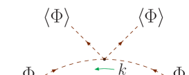
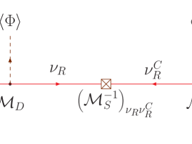
This is analogous to the type-I seesaw formula (5), which is shown diagrammatically in Figure 1. Notice that it is only the νRνRCsubscript𝜈𝑅superscriptsubscript𝜈𝑅𝐶\nu_{R}\nu_{R}^{C} component of S1superscriptsubscript𝑆1{\cal M}_{S}^{-1} that contributes to the light neutrino mass matrix at the tree level.
Refer to caption
Figure 1: The tree-level diagram for the light neutrino mass in the Inverse Seesaw Model.

In the limit μR,SMNmuch-less-thannormsubscript𝜇𝑅𝑆normsubscript𝑀𝑁||\mu_{R,S}||\ll||M_{N}||, the (1,1)11(1,1) block of S1superscriptsubscript𝑆1{\cal M}_{S}^{-1} given by (23) can be expanded in powers of μSsubscript𝜇𝑆\mu_{S}. We then obtain from (25) the tree-level light neutrino mass matrix 222Notice that μR,Snormsubscript𝜇𝑅𝑆||\mu_{R,S}|| could be bigger than MDnormsubscript𝑀𝐷||M_{D}|| in this inverse seesaw approximation.:

MνLtreesuperscriptsubscript𝑀subscript𝜈𝐿tree\displaystyle M_{\nu_{L}}^{\rm tree} =\displaystyle= MDMN1μS(MN𝖳)1MD𝖳+MDMN1μS(MN𝖳)1μRMN1μS(MN𝖳)1MD𝖳+𝒪(μS3),subscript𝑀𝐷superscriptsubscript𝑀𝑁1subscript𝜇𝑆superscriptsuperscriptsubscript𝑀𝑁𝖳1superscriptsubscript𝑀𝐷𝖳subscript𝑀𝐷superscriptsubscript𝑀𝑁1subscript𝜇𝑆superscriptsuperscriptsubscript𝑀𝑁𝖳1subscript𝜇𝑅superscriptsubscript𝑀𝑁1subscript𝜇𝑆superscriptsuperscriptsubscript𝑀𝑁𝖳1superscriptsubscript𝑀𝐷𝖳𝒪superscriptsubscript𝜇𝑆3\displaystyle M_{D}M_{N}^{-1}\mu_{S}\left(M_{N}^{\sf T}\right)^{-1}M_{D}^{\sf T}+M_{D}M_{N}^{-1}\mu_{S}\left(M_{N}^{\sf T}\right)^{-1}\mu_{R}M_{N}^{-1}\mu_{S}\left(M_{N}^{\sf T}\right)^{-1}M_{D}^{\sf T}+{\cal O}(\mu_{S}^{3})\;, (26)

which identically vanishes in the limit μS𝟎subscript𝜇𝑆0\mu_{S}\to{\bf 0}. This can also be deduced from the exact expression in (19), since in this limit, ζD𝖳=𝟎𝜁superscriptsubscript𝐷𝖳0\zeta{\cal M}_{D}^{\sf T}={\bf 0} which implies ζ=DS1𝜁subscript𝐷superscriptsubscript𝑆1\zeta={\cal M}_{D}{\cal M}_{S}^{-1} from (20), and hence, MνL=𝟎subscript𝑀subscript𝜈𝐿0M_{\nu_{L}}={\bf 0} in (19). Therefore, in this limit, the full neutrino mass matrix νsubscript𝜈{\cal M}_{\nu} in (10) has rank 6 and the light neutrinos remain massless at the tree level, even if μR𝟎subscript𝜇𝑅0\mu_{R}\neq{\bf 0}.

III Radiative Neutrino Masses and Mixings at the One-Loop Level

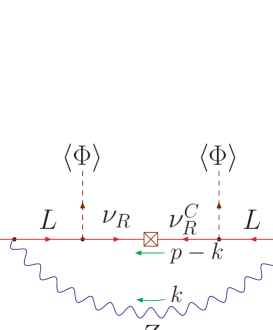
At the one-loop level, the light neutrino mass matrix MνLsubscript𝑀subscript𝜈𝐿M_{\nu_{L}} acquires a small radiative mass from the self-energy diagrams shown in Figure 2. We have drawn the figures in the flavor basis to explicitly show the lepton number violating mass insertions. Note here that the scalar propagator ΦΦ\Phi includes both the neutral Higgs boson (H𝐻H) and the neutral Goldstone boson (G0superscript𝐺0G^{0}) contributions. In the on-shell renormalization scheme and in the Feynman gauge, these are the only one-loop diagrams contributing to the neutrino mass, as in the type-I seesaw case ap92 ; Pilaftsis:2002nc ; grim2 . In a general Rξsubscript𝑅𝜉R_{\xi}-gauge parameterized by the gauge-fixing parameter ξZsubscript𝜉𝑍\xi_{Z}, the ξZsubscript𝜉𝑍\xi_{Z} dependence of the self-energy for the Z𝑍Z-loop diagram is exactly canceled by the G0superscript𝐺0G^{0}-loop diagram, and the final result is independent of ξZsubscript𝜉𝑍\xi_{Z} Pilaftsis:2002nc .

Refer to caption
Refer to caption
Figure 2: One-loop diagrams pertinent to the generation of light neutrino masses in the Minimal Radiative Inverse Seesaw Model.

The one-loop induced light neutrino masses are obtained from the momentum-dependent self-energy as follows:

MνL1loopPR=PRΣ()PR|=0,superscriptsubscript𝑀subscript𝜈𝐿1loopsubscript𝑃𝑅evaluated-atsubscript𝑃𝑅Σitalic-p̸subscript𝑃𝑅italic-p̸0\displaystyle-M_{\nu_{L}}^{\rm 1-loop}P_{R}=\left.P_{R}\Sigma(\not{p})P_{R}\right|_{\not{p}=0}~{}, (27)

where PR=(1+γ5)/2subscript𝑃𝑅1superscript𝛾52P_{R}=(1+\gamma^{5})/2 is the right-chirality projection operator. Here Σ()Σitalic-p̸\Sigma(\not{p}) is the sum of the self-energies of the diagrams shown in Figure 2, and is given by the following gauge-invariant Feynman amplitude:

PR[iΣ()]PRsubscript𝑃𝑅delimited-[]𝑖Σitalic-p̸subscript𝑃𝑅\displaystyle P_{R}[i\Sigma(\not{p})]P_{R} =\displaystyle= g2mH24mW2Dddk(2π)dPR[()𝟏6+S(pk)2𝟏6S2+iϵ][1(k2mH2+iϵ)2]PRD𝖳superscript𝑔2superscriptsubscript𝑚𝐻24superscriptsubscript𝑚𝑊2subscript𝐷superscript𝑑𝑑𝑘superscript2𝜋𝑑subscript𝑃𝑅delimited-[]italic-p̸italic-k̸subscript16subscript𝑆superscript𝑝𝑘2subscript16superscriptsubscript𝑆2𝑖italic-ϵdelimited-[]1superscriptsuperscript𝑘2superscriptsubscript𝑚𝐻2𝑖italic-ϵ2subscript𝑃𝑅superscriptsubscript𝐷𝖳\displaystyle\frac{g^{2}m_{H}^{2}}{4m_{W}^{2}}{\cal M}_{D}\int\frac{d^{d}k}{(2\pi)^{d}}P_{R}\left[\frac{(\not{p}-\not{k}){\bf 1}_{6}+{\cal M}_{S}}{(p-k)^{2}{\bf 1}_{6}-{\cal M}_{S}^{2}+i\epsilon}\right]\left[\frac{1}{(k^{2}-m_{H}^{2}+i\epsilon)^{2}}\right]P_{R}{\cal M}_{D}^{\sf T}
+g24cos2θwDddk(2π)dPRγμ[()(pk)2+iϵ][()𝟏6+S(pk)2𝟏6S2+iϵ][()(pk)2+iϵ]γνPR[gμνk2mZ2+iϵ]D𝖳,superscript𝑔24superscript2subscript𝜃𝑤subscript𝐷superscript𝑑𝑑𝑘superscript2𝜋𝑑subscript𝑃𝑅superscript𝛾𝜇delimited-[]italic-p̸italic-k̸superscript𝑝𝑘2𝑖italic-ϵdelimited-[]italic-p̸italic-k̸subscript16subscript𝑆superscript𝑝𝑘2subscript16superscriptsubscript𝑆2𝑖italic-ϵdelimited-[]italic-p̸italic-k̸superscript𝑝𝑘2𝑖italic-ϵsuperscript𝛾𝜈subscript𝑃𝑅delimited-[]subscript𝑔𝜇𝜈superscript𝑘2superscriptsubscript𝑚𝑍2𝑖italic-ϵsuperscriptsubscript𝐷𝖳\displaystyle+\frac{g^{2}}{4\cos^{2}\theta_{w}}{\cal M}_{D}\int\frac{d^{d}k}{(2\pi)^{d}}P_{R}\gamma^{\mu}\left[\frac{(\not{p}-\not{k})}{(p-k)^{2}+i\epsilon}\right]\left[\frac{(\not{p}-\not{k}){\bf 1}_{6}+{\cal M}_{S}}{(p-k)^{2}{\bf 1}_{6}-{\cal M}_{S}^{2}+i\epsilon}\right]\left[\frac{(\not{p}-\not{k})}{(p-k)^{2}+i\epsilon}\right]\gamma^{\nu}P_{R}\left[\frac{g_{\mu\nu}}{k^{2}-m_{Z}^{2}+i\epsilon}\right]{\cal M}_{D}^{\sf T}\;,

where g𝑔g is the weak gauge coupling, θwsubscript𝜃𝑤\theta_{w} is the weak mixing angle, and d=4ε𝑑4𝜀d=4-\varepsilon is the dimensionality of space-time in the dimensional regularization scheme. Notice that the integrands in (III) vanish in the infra-red (IR) limit kμ0superscript𝑘𝜇0k^{\mu}\to 0, because of the tree-level vanishing condition on light neutrino masses. However, the loop momentum k𝑘k is integrated over all possible values, and so we get a non-zero contribution to the light-neutrino mass matrix at the one-loop level. A straightforward evaluation of the ultra-violet (UV) finite Feynman integrals appearing in (III) leads to the following neutrino mass matrix in (27):

MνL1loopsuperscriptsubscript𝑀subscript𝜈𝐿1loop\displaystyle M_{\nu_{L}}^{\rm 1-loop} =\displaystyle= αW16πmW2DS[mH2S2mH2𝟏6ln(S2mH2)+3mZ2S2mZ2𝟏6ln(S2mZ2)]D𝖳,subscript𝛼𝑊16𝜋superscriptsubscript𝑚𝑊2subscript𝐷subscript𝑆delimited-[]superscriptsubscript𝑚𝐻2superscriptsubscript𝑆2superscriptsubscript𝑚𝐻2subscript16superscriptsubscript𝑆2superscriptsubscript𝑚𝐻23superscriptsubscript𝑚𝑍2superscriptsubscript𝑆2superscriptsubscript𝑚𝑍2subscript16superscriptsubscript𝑆2superscriptsubscript𝑚𝑍2superscriptsubscript𝐷𝖳\displaystyle\frac{\alpha_{W}}{16\pi m_{W}^{2}}{\cal M}_{D}{\cal M}_{S}\left[\frac{m_{H}^{2}}{{\cal M}_{S}^{2}-m_{H}^{2}{\bf 1}_{6}}\ln\left(\frac{{\cal M}_{S}^{2}}{m_{H}^{2}}\right)+\frac{3m_{Z}^{2}}{{\cal M}_{S}^{2}-m_{Z}^{2}{\bf 1}_{6}}\ln\left(\frac{{\cal M}_{S}^{2}}{m_{Z}^{2}}\right)\right]{\cal M}_{D}^{\sf T}\;, (29)

where αwg2/4πsubscript𝛼𝑤superscript𝑔24𝜋\alpha_{w}\equiv g^{2}/4\pi is the weak fine structure constant. In the limit μR,SMNmuch-less-thannormsubscript𝜇𝑅𝑆normsubscript𝑀𝑁||\mu_{R,S}||\ll||M_{N}|| and assuming that MN=mN𝟏3subscript𝑀𝑁subscript𝑚𝑁subscript13M_{N}=m_{N}{\bf 1}_{3}, for simplicity, we derive the simpler expression

MνL1loopf(xN)mW2MDμRMD𝖳,similar-to-or-equalssuperscriptsubscript𝑀subscript𝜈𝐿1loop𝑓subscript𝑥𝑁superscriptsubscript𝑚𝑊2subscript𝑀𝐷subscript𝜇𝑅superscriptsubscript𝑀𝐷𝖳\displaystyle M_{\nu_{L}}^{\rm 1-loop}\ \simeq\ \frac{f(x_{N})}{m_{W}^{2}}\;M_{D}\mu_{R}M_{D}^{\sf T}\;, (30)

where the one-loop function f(xN)𝑓subscript𝑥𝑁f(x_{N}) is given by

f(xN)𝑓subscript𝑥𝑁\displaystyle f(x_{N}) =\displaystyle= αW16π[xHxNxHln(xNxH)+3xZxNxZln(xNxZ)],subscript𝛼𝑊16𝜋delimited-[]subscript𝑥𝐻subscript𝑥𝑁subscript𝑥𝐻subscript𝑥𝑁subscript𝑥𝐻3subscript𝑥𝑍subscript𝑥𝑁subscript𝑥𝑍subscript𝑥𝑁subscript𝑥𝑍\displaystyle\frac{\alpha_{W}}{16\pi}\left[\frac{x_{H}}{x_{N}-x_{H}}\ln\left(\frac{x_{N}}{x_{H}}\right)+\ \frac{3x_{Z}}{x_{N}-x_{Z}}\ln\left(\frac{x_{N}}{x_{Z}}\right)\right], (31)

with xN=mN2/mW2subscript𝑥𝑁superscriptsubscript𝑚𝑁2superscriptsubscript𝑚𝑊2x_{N}=m_{N}^{2}/m_{W}^{2}, xH=mH2/mW2subscript𝑥𝐻superscriptsubscript𝑚𝐻2superscriptsubscript𝑚𝑊2x_{H}=m_{H}^{2}/m_{W}^{2}, xZ=mZ2/mW21/cos2θwsubscript𝑥𝑍superscriptsubscript𝑚𝑍2superscriptsubscript𝑚𝑊21superscript2subscript𝜃𝑤x_{Z}=m_{Z}^{2}/m_{W}^{2}\equiv 1/\cos^{2}\theta_{w}. From (30), we clearly see that at the one-loop level, the light neutrino mass depends linearly on the lepton number breaking term μRsubscript𝜇𝑅\mu_{R} (of dimension-3), and hence it does not vanish in the limit μS=𝟎subscript𝜇𝑆0\mu_{S}={\bf 0}, unlike at the tree level.

Refer to caption
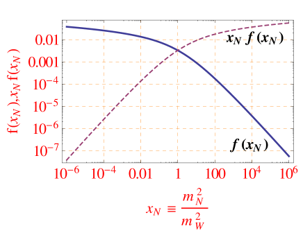
Figure 3: The analytic dependence of the one-loop function f(xN)𝑓subscript𝑥𝑁f(x_{N}) [cf. (31)] and xNf(xN)subscript𝑥𝑁𝑓subscript𝑥𝑁x_{N}f(x_{N}) on the heavy neutrino mass scale xNsubscript𝑥𝑁x_{N}.

The one-loop function f(xN)𝑓subscript𝑥𝑁f(x_{N}) given by (31) is plotted in Figure 3, for xH=1.88subscript𝑥𝐻1.88x_{H}=1.88 (corresponding to mH=125subscript𝑚𝐻125m_{H}=125 GeV), xZ=1.30subscript𝑥𝑍1.30x_{Z}=1.30 and αW=0.033subscript𝛼𝑊0.033\alpha_{W}=0.033. Note that in the limit xN1much-greater-thansubscript𝑥𝑁1x_{N}\gg 1 (as in the canonical type-I seesaw), the one-loop function stated in (31) becomes

f(xN)αW16πxH+3xZxNln(xN).similar-to-or-equals𝑓subscript𝑥𝑁subscript𝛼𝑊16𝜋subscript𝑥𝐻3subscript𝑥𝑍subscript𝑥𝑁subscript𝑥𝑁\displaystyle f(x_{N})\ \simeq\ \frac{\alpha_{W}}{16\pi}\;\frac{x_{H}+3x_{Z}}{x_{N}}\ln(x_{N})\;. (32)

Hence the light neutrino masses given by (30) are suppressed by 1/mN21superscriptsubscript𝑚𝑁21/m_{N}^{2}:

MνL1loopαW16πMDμRMD𝖳mN2mH2+3mZ2mW2ln(mN2mW2).similar-to-or-equalssubscriptsuperscript𝑀1loopsubscript𝜈𝐿subscript𝛼𝑊16𝜋subscript𝑀𝐷subscript𝜇𝑅superscriptsubscript𝑀𝐷𝖳subscriptsuperscript𝑚2𝑁superscriptsubscript𝑚𝐻23superscriptsubscript𝑚𝑍2superscriptsubscript𝑚𝑊2superscriptsubscript𝑚𝑁2superscriptsubscript𝑚𝑊2\displaystyle M^{\rm 1-loop}_{\nu_{L}}\ \simeq\ \frac{\alpha_{W}}{16\pi}\;\frac{M_{D}\mu_{R}M_{D}^{\sf T}}{m^{2}_{N}}\;\frac{m_{H}^{2}+3m_{Z}^{2}}{m_{W}^{2}}\;\ln\left(\frac{m_{N}^{2}}{m_{W}^{2}}\right). (33)

On the other hand, it is interesting to note that in the limit xN1much-less-thansubscript𝑥𝑁1x_{N}\ll 1, the one-loop function takes on the form:

f(xN)αW16πln(xHxZ3xN4).similar-to-or-equals𝑓subscript𝑥𝑁subscript𝛼𝑊16𝜋subscript𝑥𝐻superscriptsubscript𝑥𝑍3superscriptsubscript𝑥𝑁4\displaystyle f(x_{N})\ \simeq\ \frac{\alpha_{W}}{16\pi}\;\ln\left(\frac{x_{H}x_{Z}^{3}}{x_{N}^{4}}\right)\;. (34)

This leads to a light neutrino mass which is only logarithmically dependent on the heavy neutrino mass:

MνL1loopαW16πMDμRMD𝖳mW2ln(mHmZ3mN4).similar-to-or-equalssubscriptsuperscript𝑀1loopsubscript𝜈𝐿subscript𝛼𝑊16𝜋subscript𝑀𝐷subscript𝜇𝑅superscriptsubscript𝑀𝐷𝖳subscriptsuperscript𝑚2𝑊subscript𝑚𝐻superscriptsubscript𝑚𝑍3superscriptsubscript𝑚𝑁4\displaystyle M^{\rm 1-loop}_{\nu_{L}}\ \simeq\ \frac{\alpha_{W}}{16\pi}\;\frac{M_{D}\mu_{R}M_{D}^{\sf T}}{m^{2}_{W}}\;\ln\left(\frac{m_{H}m_{Z}^{3}}{m_{N}^{4}}\right)\;. (35)

It is important to stress here that this ln(mN)subscript𝑚𝑁\ln(m_{N}) dependence of the light neutrino mass is a unique feature of the Minimal Radiative Inverse Seesaw Model we have been studying here.

Finally, we wish to offer some comments on the validity of our one-loop analysis presented here. In a general study, one should also consider the loop corrections to the other mass terms appearing in the full inverse seesaw mass matrix in (10), as well as wave-function and mixing renormalizations ap96 ; Pilaftsis:2002nc . However, in the MS¯¯MS\overline{\rm MS} renormalization scheme, the UV divergences of the Dirac mass in the νLsubscript𝜈𝐿\nu_{L}νRsubscript𝜈𝑅\nu_{R} sector can be absorbed in the renormalized MDsubscript𝑀𝐷M_{D}. On the other hand, all singlet Majorana and Dirac mass matrices in the νRsubscript𝜈𝑅\nu_{R}SLsubscript𝑆𝐿S_{L} sector do not get any UV-divergent contributions, at least at the one-loop level.

IV The General Inverse Seesaw Model

Let us now consider the general inverse seesaw scenario, where both the Majorana mass matrices μSsubscript𝜇𝑆\mu_{S} and μRsubscript𝜇𝑅\mu_{R} do not vanish, i.e. μS𝟎,μR𝟎formulae-sequencesubscript𝜇𝑆0subscript𝜇𝑅0\mu_{S}\neq{\bf 0},\mu_{R}\neq{\bf 0}. To leading order in μR,Ssubscript𝜇𝑅𝑆\mu_{R,S}, the light neutrino mass matrix is given by

MνLsubscript𝑀subscript𝜈𝐿\displaystyle M_{\nu_{L}} =\displaystyle= 1mN2MD(μS+xNf(xN)μR)MD𝖳+𝒪(μS2,μR2),1superscriptsubscript𝑚𝑁2subscript𝑀𝐷subscript𝜇𝑆subscript𝑥𝑁𝑓subscript𝑥𝑁subscript𝜇𝑅superscriptsubscript𝑀𝐷𝖳𝒪superscriptsubscript𝜇𝑆2superscriptsubscript𝜇𝑅2\displaystyle\frac{1}{m_{N}^{2}}M_{D}\Big{(}\mu_{S}+x_{N}f(x_{N})\mu_{R}\Big{)}M_{D}^{\sf T}+{\cal O}(\mu_{S}^{2},\mu_{R}^{2})\;, (36)

where the one-loop function f(xN)𝑓subscript𝑥𝑁f(x_{N}) is defined in (31).

In order to get an order of magnitude estimate of the relative size of μRsubscript𝜇𝑅\mu_{R} with respect to μSsubscript𝜇𝑆\mu_{S} required to fit the neutrino oscillation data, let us choose a basis in which the charged lepton mass matrix is diagonal. Then we may write the light neutrino mass matrix as

MνL=U𝖳M^νLdiagU,subscript𝑀subscript𝜈𝐿superscript𝑈𝖳superscriptsubscript^𝑀subscript𝜈𝐿diag𝑈\displaystyle M_{\nu_{L}}\ =\ U^{\sf T}\widehat{M}_{\nu_{L}}^{\rm diag}U\;, (37)

where U𝑈U is the PMNS mixing matrix333For simplicity, we have not considered here the leptonic non-unitarity effects which are generally of order ζnorm𝜁||\zeta|| in inverse seesaw models nuty . given in terms of the three mixing angles, one Dirac and two Majorana CP𝐶𝑃CP phases vureview :

U=(c12c13s12c13s13eiδs12c23c12s23s13eiδc12c23s12s23s13eiδs23c13s12s23c12c23s13eiδc12s23s12c23s13eiδc23c13)×diag(eiα1/2,eiα2/2,1),𝑈subscript𝑐12subscript𝑐13subscript𝑠12subscript𝑐13subscript𝑠13superscript𝑒𝑖𝛿subscript𝑠12subscript𝑐23subscript𝑐12subscript𝑠23subscript𝑠13superscript𝑒𝑖𝛿subscript𝑐12subscript𝑐23subscript𝑠12subscript𝑠23subscript𝑠13superscript𝑒𝑖𝛿subscript𝑠23subscript𝑐13subscript𝑠12subscript𝑠23subscript𝑐12subscript𝑐23subscript𝑠13superscript𝑒𝑖𝛿subscript𝑐12subscript𝑠23subscript𝑠12subscript𝑐23subscript𝑠13superscript𝑒𝑖𝛿subscript𝑐23subscript𝑐13diagsuperscript𝑒𝑖subscript𝛼12superscript𝑒𝑖subscript𝛼221\displaystyle U=\left(\begin{array}[]{ccc}c_{12}c_{13}&s_{12}c_{13}&s_{13}e^{-i\delta}\\ -s_{12}c_{23}-c_{12}s_{23}s_{13}e^{i\delta}&c_{12}c_{23}-s_{12}s_{23}s_{13}e^{i\delta}&s_{23}c_{13}\\ s_{12}s_{23}-c_{12}c_{23}s_{13}e^{i\delta}&-c_{12}s_{23}-s_{12}c_{23}s_{13}e^{i\delta}&c_{23}c_{13}\end{array}\right)\times{\rm diag}(e^{i\alpha_{1}/2},e^{i\alpha_{2}/2},1)\;, (41)

with cijcosθij,sijsinθijformulae-sequencesubscript𝑐𝑖𝑗subscript𝜃𝑖𝑗subscript𝑠𝑖𝑗subscript𝜃𝑖𝑗c_{ij}\equiv\cos\theta_{ij},s_{ij}\equiv\sin\theta_{ij}. For a normal hierarchy, one has

M^νLdiag=diag(m1,Δmsol2,Δmatm2).superscriptsubscript^𝑀subscript𝜈𝐿diagdiagsubscript𝑚1Δsubscriptsuperscript𝑚2solΔsubscriptsuperscript𝑚2atm\displaystyle\widehat{M}_{\nu_{L}}^{\rm diag}={\rm diag}(m_{1},\sqrt{\Delta m^{2}_{\rm sol}},\sqrt{\Delta m^{2}_{\rm atm}})\;. (42)

Using the central values of a recent global-fit analysis of the neutrino oscillation parameters global :

Δmsol2=7.62×10⁵eV2,Δmatm2=2.55×10³eV2,θ12=34.4,θ23=40.8,θ13=9.0,δ=0.8π,formulae-sequenceΔsubscriptsuperscript𝑚2sol7.62superscript105superscripteV2formulae-sequenceΔsubscriptsuperscript𝑚2atm2.55superscript103superscripteV2formulae-sequencesubscript𝜃12superscript34.4formulae-sequencesubscript𝜃23superscript40.8formulae-sequencesubscript𝜃13superscript9.0𝛿0.8𝜋\displaystyle\Delta m^{2}_{\rm sol}=7.62\times 10^{-5}~{}{\rm eV}^{2},~{}\Delta m^{2}_{\rm atm}=2.55\times 10^{-3}~{}{\rm eV}^{2},~{}\theta_{12}=34.4^{\circ},~{}\theta_{23}=40.8^{\circ},\theta_{13}=9.0^{\circ},\delta=0.8\pi\;, (43)

and assuming m1=0,α1=α2=0formulae-sequencesubscript𝑚10subscript𝛼1subscript𝛼20m_{1}=0,\alpha_{1}=\alpha_{2}=0, we obtain from (37):

MνLsubscript𝑀subscript𝜈𝐿\displaystyle M_{\nu_{L}} =\displaystyle= (102eV)×(0.310.12i0.09+0.32i0.72+0.37i0.09+0.32i2.53+0.04i2.19+0.01i0.72+0.37i2.19+0.01i3.070.03i).superscript102eV0.310.12𝑖0.090.32𝑖0.720.37𝑖0.090.32𝑖2.530.04𝑖2.190.01𝑖0.720.37𝑖2.190.01𝑖3.070.03𝑖\displaystyle(10^{-2}~{}{\rm eV})\times\left(\begin{array}[]{ccc}0.31-0.12i&-0.09+0.32i&-0.72+0.37i\\ -0.09+0.32i&2.53+0.04i&2.19+0.01i\\ -0.72+0.37i&2.19+0.01i&3.07-0.03i\end{array}\right). (47)

For illustration, let us absorb the flavor structure of MDsubscript𝑀𝐷M_{D} in (36) into the matrices μR,Ssubscript𝜇𝑅𝑆\mu_{R,S}, by rewriting the light-neutrino mass matrix as

MνL=λD(μ¯S+xNf(xN)μ¯R)λDμ¯eff,subscript𝑀subscript𝜈𝐿subscript𝜆𝐷subscript¯𝜇𝑆subscript𝑥𝑁𝑓subscript𝑥𝑁subscript¯𝜇𝑅subscript𝜆𝐷subscript¯𝜇eff\displaystyle M_{\nu_{L}}\ =\ \lambda_{D}\,\Big{(}\bar{\mu}_{S}+x_{N}f(x_{N})\bar{\mu}_{R}\,\Big{)}\ \equiv\ \lambda_{D}\bar{\mu}_{\rm eff}\;, (48)

where λD=mDmax2/mN2subscript𝜆𝐷superscriptsubscript𝑚subscript𝐷max2superscriptsubscript𝑚𝑁2\lambda_{D}=m_{D_{\rm max}}^{2}/m_{N}^{2} and mDmax=max(|(MD)ij|)subscript𝑚subscript𝐷maxmaxsubscriptsubscript𝑀𝐷𝑖𝑗m_{D_{\rm max}}={\rm max}\left(|(M_{D})_{ij}|\right) is the largest element of MDsubscript𝑀𝐷M_{D} (in absolute-value terms). In addition, we have re-defined μS,Rsubscript𝜇𝑆𝑅\mu_{S,R} as

μ¯S=KμSK𝖳,μ¯R=KμRK𝖳,formulae-sequencesubscript¯𝜇𝑆𝐾subscript𝜇𝑆superscript𝐾𝖳subscript¯𝜇𝑅𝐾subscript𝜇𝑅superscript𝐾𝖳\displaystyle\bar{\mu}_{S}\ =\ K\mu_{S}K^{\sf T}\;,\qquad\bar{\mu}_{R}\ =\ K\mu_{R}K^{\sf T}\;, (49)

where K=MD/mDmax𝐾subscript𝑀𝐷subscript𝑚subscript𝐷maxK=M_{D}/m_{D_{\rm max}} is in general a dimensionless 3×3333\times 3 complex matrix. With these definitions, we can now make a one-to-one mapping between the elements of MνLsubscript𝑀subscript𝜈𝐿M_{\nu_{L}} and μ¯R,Ssubscript¯𝜇𝑅𝑆\bar{\mu}_{R,S}.

Refer to caption
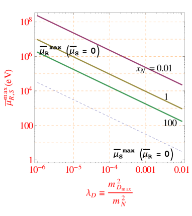
Figure 4: The magnitudes of the largest element of μ¯Ssubscript¯𝜇𝑆\bar{\mu}_{S} (dashed line) and μ¯Rsubscript¯𝜇𝑅\bar{\mu}_{R} (solid lines for various values of xNsubscript𝑥𝑁x_{N}) as a function of the ratio λDsubscript𝜆𝐷\lambda_{D}.

This is shown in Figure 4 where we have plotted against the ratio λDsubscript𝜆𝐷\lambda_{D}: (i) the magnitude of the largest entry in μ¯Ssubscript¯𝜇𝑆\bar{\mu}_{S} (denoted as μ¯Smaxsuperscriptsubscript¯𝜇𝑆max\bar{\mu}_{S}^{\rm max}) for μ¯R=𝟎subscript¯𝜇𝑅0\bar{\mu}_{R}={\bf 0} (the dashed line); (ii) the magnitude of the largest entry in μ¯Rsubscript¯𝜇𝑅\bar{\mu}_{R} (denoted as μ¯Smaxsuperscriptsubscript¯𝜇𝑆max\bar{\mu}_{S}^{\rm max}) for μ¯S=𝟎subscript¯𝜇𝑆0\bar{\mu}_{S}={\bf 0} and for xN=0.01,1,100subscript𝑥𝑁0.011100x_{N}=0.01,1,100 (the solid lines). We note that the mass scale of μRmaxsuperscriptsubscript𝜇𝑅max\mu_{R}^{\rm max} is roughly 222444 orders of magnitude larger than that of μSmaxsuperscriptsubscript𝜇𝑆max\mu_{S}^{\rm max}. Thus, if μR𝟎subscript𝜇𝑅0\mu_{R}\neq{\bf 0}, a much milder hierarchy can be realized between the lepton-number breaking scale μRmaxsuperscriptsubscript𝜇𝑅max\mu_{R}^{\rm max} and the electroweak scale mWsubscript𝑚𝑊m_{W} in the Minimal Radiative Inverse Seesaw Model.

In the general inverse seesaw scenario where μR,S𝟎subscript𝜇𝑅𝑆0\mu_{R,S}\neq{\bf 0}, the mass matrix μ¯effsubscript¯𝜇eff\bar{\mu}_{\rm eff} defined by (48):

μ¯eff=μ¯S+xNf(xN)μ¯R,subscript¯𝜇effsubscript¯𝜇𝑆subscript𝑥𝑁𝑓subscript𝑥𝑁subscript¯𝜇𝑅\displaystyle\bar{\mu}_{\rm eff}=\bar{\mu}_{S}+x_{N}f(x_{N})\bar{\mu}_{R}, (50)

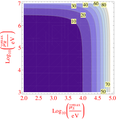
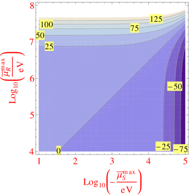
is fixed by the neutrino oscillation data for a given value of λDsubscript𝜆𝐷\lambda_{D}. The dependence of μ¯effmaxsuperscriptsubscript¯𝜇effmax\bar{\mu}_{\rm eff}^{\rm max} on λDsubscript𝜆𝐷\lambda_{D} is exactly the same as that of μ¯Smaxsuperscriptsubscript¯𝜇𝑆max\bar{\mu}_{S}^{\rm max} (with μ¯R=𝟎subscript¯𝜇𝑅0\bar{\mu}_{R}={\bf 0}), as shown by the dashed line in Figure 4. However, the relative size between μRsubscript𝜇𝑅\mu_{R} and μSsubscript𝜇𝑆\mu_{S} depends on their relative sign, for a fixed given ratio xNsubscript𝑥𝑁x_{N}. For instance, when both μ¯Smax,μ¯Rmax>0superscriptsubscript¯𝜇𝑆maxsuperscriptsubscript¯𝜇𝑅max0\bar{\mu}_{S}^{\rm max},\bar{\mu}_{R}^{\rm max}>0, the constant contours of μ¯effmaxsuperscriptsubscript¯𝜇effmax\bar{\mu}_{\rm eff}^{\rm max} (in keV) are shown in Figure 5 for xN=1subscript𝑥𝑁1x_{N}=1. For μ¯Smax<0superscriptsubscript¯𝜇𝑆max0\bar{\mu}_{S}^{\rm max}<0 and μ¯Rmax>0superscriptsubscript¯𝜇𝑅max0\bar{\mu}_{R}^{\rm max}>0, the corresponding contours are shown in Figure 6, where we have the cancellation regions (μ¯effmax0superscriptsubscript¯𝜇effmax0\bar{\mu}_{\rm eff}^{\rm max}\to 0) for certain combinations of (μ¯Smax,μ¯Rmax)superscriptsubscript¯𝜇𝑆maxsuperscriptsubscript¯𝜇𝑅max\left(\bar{\mu}_{S}^{\rm max},\bar{\mu}_{R}^{\rm max}\right).

Refer to caption
Figure 5: Contours of constant μ¯effmaxsuperscriptsubscript¯𝜇effmax\bar{\mu}_{\rm eff}^{\rm max} (in keV) for xN=1subscript𝑥𝑁1x_{N}=1 and for μ¯R,Smax>0superscriptsubscript¯𝜇𝑅𝑆max0\bar{\mu}_{R,S}^{\rm max}>0.
Refer to caption
Figure 6: Contours of constant μ¯effmaxsuperscriptsubscript¯𝜇effmax\bar{\mu}_{\rm eff}^{\rm max} (in keV) for xN=1subscript𝑥𝑁1x_{N}=1 and for μ¯Smax<0,μ¯Rmax>0formulae-sequencesuperscriptsubscript¯𝜇𝑆max0superscriptsubscript¯𝜇𝑅max0\bar{\mu}_{S}^{\rm max}<0,~{}\bar{\mu}_{R}^{\rm max}>0.

We conclude this section by commenting that our numerical results only depend on the largest element of the light neutrino mass matrix which is always of the order of Δmatm2Δsubscriptsuperscript𝑚2atm\sqrt{\Delta m^{2}_{\rm atm}}, irrespective of the neutrino mass hierarchy. Hence our order of magnitude estimates will be valid for an inverted hierarchical light neutrino mass spectrum as well.

V Conclusions

We have presented a minimal radiative mechanism for generating light neutrino masses in inverse seesaw models. The radiative neutrino masses arise at the one-loop level from known SM electroweak quantum effects involving the Z𝑍Z and Higgs bosons. Unlike in other radiative inverse seesaw mechanisms existing in the literature radiative , the implementation of our radiative mechanism does not require any extra non-standard fields other than usual SM singlet neutrinos.

In the Minimal Radiative Inverse Seesaw Model, where the dimension-3 lepton-number breaking mass matrix μRsubscript𝜇𝑅\mu_{R} of the right-handed neutrinos is non-zero, we have found that the light neutrino masses generated at one-loop level are UV-finite and are directly proportional to μRsubscript𝜇𝑅\mu_{R}. We also showed that the 3-by-3 Majorana mass matrix μRsubscript𝜇𝑅\mu_{R} could be 24242-4 orders of magnitude larger than the other 3-by-3 Majorana mass matrix μSsubscript𝜇𝑆\mu_{S} present in the standard inverse seesaw models. Hence, this could alleviate the hierarchy between the lepton number breaking scale and the electroweak scale in these models. In a supersymmetric version of this mechanism (e.g., susy ), one might expect to ameliorate this hierarchy even further, in addition to having a scalar dark matter candidate in the form of the lightest sneutrino dm . We hope to return to these issues in a future communication.

Acknowledgements.
This work is supported in part by the Lancaster-Manchester-Sheffield Consortium for Fundamental Physics under STFC grant ST/J000418/1. In addition, AP gratefully acknowledges partial support by a IPPP associateship from Durham University.

References

  • (1) For a review, see, e.g. K. Nakamura and S. T. Petcov, in J. Beringer et al. (PDG), Phys. Rev. D86, 010001 (2012) (http://pdg.lbl.gov).
  • (2) S. Weinberg, Phys. Rev. Lett. 43, 1566 (1979).
  • (3) P. Minkowski, Phys. Lett. B67, 421 (1977); T. Yanagida, in Workshop on Unified Theories, KEK Report 79-18, p. 95 (1979); M. Gell-Mann, P. Ramond and R. Slansky, in Supergravity, P. van Nieuwenhuizen and D. Z. Freedman (eds.), North Holland, Amsterdam (1979), p. 315; R. N. Mohapatra and G. Senjanovic, Phys. Rev. Lett. 44, 912 (1980).
  • (4) M. Magg and C. Wetterich, Phys. Lett. B 94, 61 (1980); J. Schechter and J. W. F. Valle, Phys. Rev. D 22, 2227 (1980); T. P. Cheng and L. -F. Li, Phys. Rev. D 22, 2860 (1980); G. Lazarides, Q. Shafi and C. Wetterich, Nucl. Phys. B 181, 287 (1981); R. N. Mohapatra and G. Senjanovic, Phys. Rev. D 23, 165 (1981).
  • (5) R. Foot, H. Lew, X. G. He and G. C. Joshi, Z. Phys. C 44, 441 (1989).
  • (6) A. Pilaftsis, Phys. Rev. Lett. 95, 081602 (2005) [hep-ph/0408103]; A. Pilaftsis and T. E. J. Underwood, Phys. Rev. D72, 113001 (2005) [hep- ph/0506107]; J. Kersten and A. Y. Smirnov, Phys. Rev.  D76, 073005 (2007) [arXiv:0705.3221 [hep-ph]]; A. de Gouvea, arXiv:0706.1732 [hep-ph]; X. G. He, S. Oh, J. Tandean, and C. C. Wen, Phys. Rev. D 80, 073012 (2009) [arXiv:0907.1607 [hep-ph]].
  • (7) R. N. Mohapatra, Phys. Rev. Lett.  56, 561 (1986); R. N. Mohapatra and J. W. F. Valle, Phys. Rev. D34, 1642 (1986).
  • (8) D. Wyler and L. Wolfenstein, Nucl. Phys. B 218, 205 (1983); E. K. Akhmedov, M. Lindner, E. Schnapka and J. W. F. Valle, Phys. Lett. B 368, 270 (1996) [hep-ph/9507275]; ibid., Phys. Rev. D 53, 2752 (1996) [hep-ph/9509255]; M. Malinsky, J. C. Romao and J. W. F. Valle, Phys. Rev. Lett.  95, 161801 (2005) [hep-ph/0506296].
  • (9) E. Ma, Mod. Phys. Lett. A 24, 2161 (2009) [arXiv:0904.1580 [hep-ph]].
  • (10) A. Pilaftsis, Z. Phys. C 55, 275 (1992) [hep-ph/9901206].
  • (11) J. G. Korner, A. Pilaftsis and K. Schilcher, Phys. Rev. D 47, 1080 (1993) [hep-ph/9301289].
  • (12) A. Pilaftsis, Phys. Rev. D 78, 013008 (2008) [arXiv:0805.1677 [hep-ph]].
  • (13) W. Grimus and L. Lavoura, JHEP 0011, 042 (2000) [hep-ph/0008179]; H. Hettmansperger, M. Lindner and W. Rodejohann, JHEP 1104, 123 (2011) [arXiv:1102.3432 [hep-ph]].
  • (14) A. Pilaftsis, Phys. Rev. D 65, 115013 (2002) [hep-ph/0203210].
  • (15) W. Grimus and L. Lavoura, Phys. Lett. B 546, 86 (2002) [hep-ph/0207229]; D. Aristizabal Sierra and C. E. Yaguna, JHEP 1108, 013 (2011) [arXiv:1106.3587 [hep-ph]].
  • (16) B. A. Kniehl and A. Pilaftsis, Nucl. Phys. B 474, 286 (1996) [hep-ph/9601390].
  • (17) M. Malinsky, T. Ohlsson and H. Zhang, Phys. Rev. D 79, 073009 (2009) [arXiv:0903.1961 [hep-ph]]; M. Malinsky, T. Ohlsson, Z. -z. Xing and H. Zhang, Phys. Lett. B 679, 242 (2009) [arXiv:0905.2889 [hep-ph]]; P. S. B. Dev and R. N. Mohapatra, Phys. Rev. D 81, 013001 (2010) [arXiv:0910.3924 [hep-ph]].
  • (18) D. V. Forero, M. Tortola and J. W. F. Valle, arXiv:1205.4018 [hep-ph].
  • (19) E. Ma, Phys. Rev. D 80, 013013 (2009) [arXiv:0904.4450 [hep-ph]]; F. Bazzocchi, D. G. Cerdeno, C. Munoz and J. W. F. Valle, Phys. Rev. D 81, 051701 (2010) [arXiv:0907.1262 [hep-ph]]; S. S. C. Law and K. L. McDonald, Phys. Lett. B 713, 490 (2012) [arXiv:1204.2529 [hep-ph]]; H. Okada and T. Toma, arXiv:1207.0864 [hep-ph]; G. Guo, X. -G. He and G. -N. Li, arXiv:1207.6308 [hep-ph].
  • (20) F. Deppisch and J. W. F. Valle, Phys. Rev. D 72, 036001 (2005) [hep-ph/0406040]; M. Hirsch, T. Kernreiter, J. C. Romao and A. Villanova del Moral, JHEP 1001, 103 (2010) [arXiv:0910.2435 [hep-ph]].
  • (21) C. Arina, F. Bazzocchi, N. Fornengo, J. C. Romao, J. W. F. Valle, Phys. Rev. Lett. 101, 161802 (2008) [arXiv:0806.3225 [hep-ph]]; S. Khalil, H. Okada, T. Toma, JHEP 1107, 026 (2011) [arXiv:1102.4249 [hep-ph]]; F. -X. Josse-Michaux and E. Molinaro, Phys. Rev. D 84, 125021 (2011) [arXiv:1108.0482 [hep-ph]]; H. An, P. S. B. Dev, Y. Cai and R. N. Mohapatra, Phys. Rev. Lett. 108, 081806 (2012) [arXiv:1110.1366 [hep-ph]].