The Electroweak Fit of the Standard Model
after the Discovery of a New Boson at the LHC

The Gfitter Group
M. Baak^a, M. Goebel^b, J. Haller^c, A. Hoecker^a, D. Kennedy^b,
R. Kogler^c, K. Mönig^b, M. Schott^a, J. Stelzer^d

^aCERN, Geneva, Switzerland
^bDESY, Hamburg and Zeuthen, Germany
^cInstitut für Experimentalphysik, Universität Hamburg, Germany
^dDepartment of Physics and Astronomy, Michigan State University, East Lansing, USA

• Abstract — In view of the discovery of a new boson by the ATLAS and CMS Collaborations at the LHC, we present an update of the global Standard Model (SM) fit to electroweak precision data. Assuming the new particle to be the SM Higgs boson, all fundamental parameters of the SM are known allowing, for the first time, to overconstrain the SM at the electroweak scale and assert its validity. Including the effects of radiative corrections and the experimental and theoretical uncertainties, the global fit exhibits a $p$-value of 0.07. The mass measurements by ATLAS and CMS agree within 1.3$\sigma$ with the indirect determination $M_{H}=94^{\,+25}_{\,-22}$ GeV. Within the SM the $W$ boson mass and the effective weak mixing angle can be accurately predicted to be $M_{W}=80.359\pm 0.011\>\mathrm{Ge\kern-0.90005ptV}$ and $\sin\!^{2}\theta^{\ell}_{{\rm eff}}=0.23150\pm 0.00010$ from the global fit. These results are compatible with, and exceed in precision, the direct measurements. For the indirect determination of the top quark mass we find $m_{t}=175.8^{\>+2.7}_{\>-2.4}\>\mathrm{Ge\kern-0.90005ptV}$, in agreement with the kinematic and cross-section based measurements.

1 Introduction

The discovery by the ATLAS [1] and CMS [2] experiments at the LHC of a new particle with mass $\sim$126 $\mathrm{Ge\kern-1.00006ptV}$ and with properties compatible with those of the Standard Model (SM) Higgs boson concludes decades of intense experimental and theoretical work to uncover the mechanism of electroweak symmetry breaking and mass generation. If forthcoming data confirm that the new particle is the SM Higgs boson, this discovery exhibits another – possibly the greatest ever – triumph of the SM, as not only the SM predicts the Higgs couplings to the SM fermions and bosons, but it also constrains the Higgs boson to be light compared to its unitarity bound of roughly a TeV. This indirect information on the Higgs mass was extracted from Higgs loops affecting the values of $Z$ boson asymmetry observables and the $W$ mass. Global fits to precisely measured electroweak data derived 95% confidence level (CL) upper limits on the Higgs mass of around 160 $\mathrm{Ge\kern-1.00006ptV}$ [3, 4, 5, 6].

In this letter we interpret the new particle as the SM Higgs boson and present the consequences on the global electroweak fit. A detailed description of the experimental data, the theoretical calculations, and the statistical framework used in the analysis is provided in past publications [7, 6]. Here, we only briefly recall the most relevant aspects of the analysis and highlight recent changes. The main goal of this letter is to quantify the compatibility of the mass of the discovered boson with the electroweak precision data and its impact on the indirect determination of the $W$ boson mass, the effective weak mixing angle, and the top quark mass. The implications of the discovery on the SM with three and four fermion generations were also studied in [8].

2 Experimental data and theoretical predictions

The experimental inputs used in the fit include the electroweak precision data measured at the $Z$ pole and their correlations [9], the latest world average values for the mass of the $W$ boson, $M_{W}=80.385\pm 0.015\>\mathrm{Ge\kern-1.00006ptV}$ [10], and its width, $\Gamma_{W}=2.085\pm 0.042\>\mathrm{Ge\kern-1.00006ptV}$ [11], the latest average of the direct top mass measurements from the Tevatron experiments, $m_{t}=173.18\pm 0.94\>\mathrm{Ge\kern-1.00006ptV}$ [12], and the hadronic contribution to the running of the electromagnetic coupling strength, $\Delta\alpha_{\rm had}^{(5)}(M_{Z}^{2})=(2757\pm 10)\cdot 10^{-5}$ [19]. For the Higgs boson mass we use the measurements from ATLAS, $M_{H}=126.0\pm 0.4\pm 0.4\>\mathrm{Ge\kern-1.00006ptV}$ [1], and CMS, $M_{H}=125.3\pm 0.4\pm 0.5\>\mathrm{Ge\kern-1.00006ptV}$ [2], where the first uncertainties are statistical and the second systematic. A detailed list of all the observables, their values and uncertainties as used in the fit, is given in the first two columns of Table 1.

A proper average of the Higgs mass measurements requires a detailed experimental study of the systematic correlations. Owing to the weak (logarithmic) dependence of the electroweak fit on the Higgs mass, we find that the fit results are insensitive to the difference between a straight (uncorrelated) weighted average of the ATLAS and CMS measurements ($M_{H}=125.7\pm 0.4$ GeV), and their weighted average obtained assuming the systematic uncertainties to be fully correlated ($M_{H}=125.7\pm 0.5$ GeV). In this paper the former combination is used.

For the theoretical predictions, we use the calculations detailed in [6] and references therein. They feature among others the complete $\mathcal{O}(\alpha_{\scriptscriptstyle S}^{4})$ calculation of the QCD Adler function [20, 21] and the full two-loop and leading beyond-two-loop prediction of the $W$ mass and the effective weak mixing angle [22, 23, 24]. Two modifications apply here: first, an improved prediction of $R^{0}_{b}$ is invoked that includes the calculation of the complete fermionic electroweak two-loop (NNLO) corrections based on numerical Mellin-Barnes integrals [25]; second, the calculation of the vector and axial-vector couplings, $g_{A}^{f}$ and $g_{V}^{f}$, now entirely relies on accurate parametrisations [26, 27, 28, 29]; the correction factors from a comparison with the Fortran ZFITTER package [30, 31] applied previously at very high Higgs masses [6] are no longer used.

3 Results

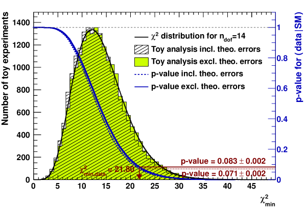
The fit to all input data from Table 1 converges with a global minimum value for the test statistics of $\chi^{2}_{{\rm min}}=21.8$, obtained for $14$ degrees of freedom. Using a pseudo Monte Carlo (MC) simulation and the statistical method described in [7] we find the $\chi^{2}_{{\rm min}}$ distribution shown in Fig. 1. The resulting $p$-value for the SM to describe the data amounts to $0.07$ (corresponding to $1.8\sigma$). This result is consistent with the naive $p$-value ${\rm Prob}(21.8,14)=0.08$.

The inferior compatibility of the fit compared to earlier results [6] is not primarily caused by the insertion of the new $M_{H}$ measurements in the fit, but is due to the usage of a more accurate $R^{0}_{b}$ calculation [25] that leads to a smaller SM prediction.

		Free	Fit result	Fit result	Fit result incl. $M_{H}$
Parameter	Input value	in fit	incl. $M_{H}$	not incl. $M_{H}$	but not exp. input in row
$M_{H}$ [GeV](∘)	$125.7\pm 0.4$	yes	$125.7\pm 0.4$	$94^{\,+25}_{\,-22}$	$94^{\,+25}_{\,-22}$
$M_{W}$ [GeV]	$80.385\pm 0.015$	–	$80.367\pm 0.007$	$80.380\pm 0.012$	$80.359\pm 0.011$
$\Gamma_{W}$ [GeV]	$2.085\pm 0.042$	–	$2.091\pm 0.001$	$2.092\pm 0.001$	$2.091\pm 0.001$
$M_{Z}$ [GeV]	$91.1875\pm 0.0021$	yes	$91.1878\pm 0.0021$	$91.1874\pm 0.0021$	$91.1983\pm 0.0116$
$\Gamma_{Z}$ [GeV]	$2.4952\pm 0.0023$	–	$2.4954\pm 0.0014$	$2.4958\pm 0.0015$	$2.4951\pm 0.0017$
$\sigma_{\rm had}^{0}$ [nb]	$41.540\pm 0.037$	–	$41.479\pm 0.014$	$41.478\pm 0.014$	$41.470\pm 0.015$
$R^{0}_{\ell}$	$20.767\pm 0.025$	–	$20.740\pm 0.017$	$20.743\pm 0.018$	$20.716\pm 0.026$
$A_{\rm FB}^{0,\ell}$	$0.0171\pm 0.0010$	–	$0.01627\pm 0.0002$	$0.01637\pm 0.0002$	$0.01624\pm 0.0002$
$A_{\ell}$ (⋆)	$0.1499\pm 0.0018$	–	$0.1473^{\,+0.0006}_{\,-0.0008}$	$0.1477\pm 0.0009$	$0.1468\pm 0.0005$(†)
$\sin\!^{2}\theta^{\ell}_{{\rm eff}}(Q_{\rm FB})$	$0.2324\pm 0.0012$	–	$0.23148^{\,+0.00011}_{\,-0.00007}$	$0.23143^{\,+0.00010}_{\,-0.00012}$	$0.23150\pm 0.00009$
$A_{c}$	$0.670\pm 0.027$	–	$0.6680^{\,+0.00025}_{\,-0.00038}$	$0.6682^{\,+0.00042}_{\,-0.00035}$	$0.6680\pm 0.00031$
$A_{b}$	$0.923\pm 0.020$	–	$0.93464^{\,+0.00004}_{\,-0.00007}$	$0.93468\pm 0.00008$	$0.93463\pm 0.00006$
$A_{\rm FB}^{0,c}$	$0.0707\pm 0.0035$	–	$0.0739^{\,+0.0003}_{\,-0.0005}$	$0.0740\pm 0.0005$	$0.0738\pm 0.0004$
$A_{\rm FB}^{0,b}$	$0.0992\pm 0.0016$	–	$0.1032^{\,+0.0004}_{\,-0.0006}$	$0.1036\pm 0.0007$	$0.1034\pm 0.0004$
$R^{0}_{c}$	$0.1721\pm 0.0030$	–	$0.17223\pm 0.00006$	$0.17223\pm 0.00006$	$0.17223\pm 0.00006$
$R^{0}_{b}$	$0.21629\pm 0.00066$	–	$0.21474\pm 0.00003$	$0.21475\pm 0.00003$	$0.21473\pm 0.00003$
$\overline{m}_{c}$ [GeV]	$1.27^{\,+0.07}_{\,-0.11}$	yes	$1.27^{\,+0.07}_{\,-0.11}$	$1.27^{\,+0.07}_{\,-0.11}$	–
$\overline{m}_{b}$ [GeV]	$4.20^{\,+0.17}_{\,-0.07}$	yes	$4.20^{\,+0.17}_{\,-0.07}$	$4.20^{\,+0.17}_{\,-0.07}$	–
$m_{t}$ [GeV]	$173.18\pm 0.94$	yes	$173.52\pm 0.88$	$173.14\pm 0.93$	$175.8^{\,+2.7}_{\,-2.4}$
$\Delta\alpha_{\rm had}^{(5)}(M_{Z}^{2})$ (△▽)	$2757\pm 10$	yes	$2755\pm 11$	$2757\pm 11$	$2716^{\,+49}_{\,-43}$
$\alpha_{\scriptscriptstyle S}(M_{Z}^{2})$	–	yes	$0.1191\pm 0.0028$	$0.1192\pm 0.0028$	$0.1191\pm 0.0028$
$\delta_{\rm th}M_{W}$ [MeV]	$[-4,4]_{\rm theo}$	yes	$4$	$4$	–
$\delta_{\rm th}\sin\!^{2}\theta^{\ell}_{{\rm eff}}$ (△)	$[-4.7,4.7]_{\rm theo}$	yes	$-1.4$	$4.7$	–

^(∘)Average of ATLAS ($M_{H}=126.0\pm 0.4~{}(\rm{stat})\pm 0.4~{}(\rm{sys})$) and CMS ($M_{H}=125.3\pm 0.4~{}(\rm{stat})\pm 0.5~{}(\rm{sys})$) measurements assuming no correlation of the systematic uncertainties (see discussion in Sect. 2). ^(⋆)Average of LEP ($A_{\ell}=0.1465\pm 0.0033$) and SLD ($A_{\ell}=0.1513\pm 0.0021$) measurements, used as two measurements in the fit. ^(†)The fit w/o the LEP (SLD) measurement gives $A_{\ell}=$ $0.1474^{\,+0.0005}_{\,-0.0009}$ ($A_{\ell}=$ $0.1467^{\,+0.0006}_{\,-0.0004}$).

^(△)In units of $10^{-5}$. ^(▽)Rescaled due to $\alpha_{\scriptscriptstyle S}$ dependency.

Table 1: Input values and fit results for the observables and parameters of the global electroweak fit. The first and second columns list respectively the observables/parameters used in the fit, and their experimental values or phenomenological estimates (see text for references). The subscript “theo” labels theoretical error ranges. The third column indicates whether a parameter is floating in the fit. The fourth column quotes the results of the complete fit including all experimental data. The fifth column gives the fit results for each parameter without using the $M_{H}$ measurement in the fit. In the last column the fit results are given without using the corresponding experimental or phenomenological estimate in the given row.

Figure 1: Result of a pseudo MC analysis of the complete electroweak fit. Shown are distributions of the $\chi^{2}_{{\rm min}}$ test statistics obtained from a pseudo MC simulation with varying (hatched histogram) and fixed theoretical uncertainty parameters ($\delta_{\rm th}$) in the fit (shaded/green histogram). The $\chi^{2}_{{\rm min}}$ obtained in the complete fit to data is indicted by the arrow together with the $p$-values found for these two cases. Also shown is an idealised $\chi^{2}$ function assuming a Gaussian case with 14 degrees of freedom (solid black line).

Figure 2: Left: pull comparison of the fit results with the direct measurements in units of the experimental uncertainty. Right: determination of $M_{H}$ excluding the direct $M_{H}$ measurements and all the sensitive observables from the fit, except the one given. Note that the fit results shown are not independent.

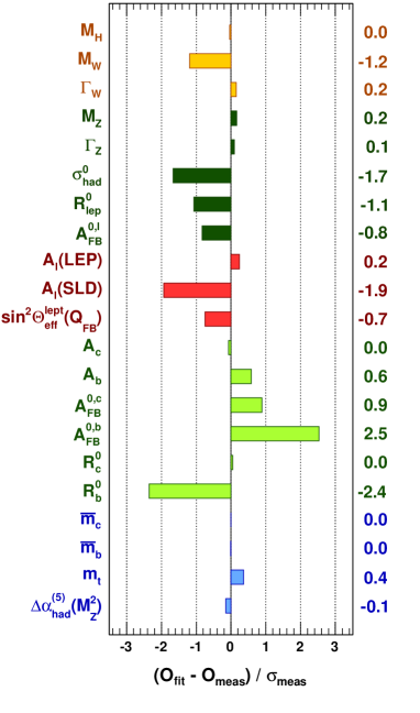
The results of the complete fit for each fit parameter and observable are given in the fourth column of Table 1, together with their uncertainties estimated from their $\Delta\chi^{2}=1$ profiles. Figure 2 (left) shows the pull values obtained from the difference between the result of the fit and the input data in units of the data uncertainty. No single pull value exceeds $3\sigma$. The known tension between the left-right asymmetry and $A_{\rm FB}^{0,b}$ is reproduced. The new $R_{b}^{0}$ calculation [25] increases the discrepancy between the $R_{b}^{0}$ prediction and its measurement from $-0.8\sigma$ to $-2.4\sigma$.

The fifth column in Table 1 gives the results obtained without using the $M_{H}$ measurements in the fit (i.e., $M_{H}$ is a freely varying parameter). In this case, which represents the well known result of the standard electroweak fit prior to the $M_{H}$ measurement, the fit converges with a global minimum of $\chi^{2}_{{\rm min}}=20.3$ for 13 degrees of freedom (${\rm Prob}(20.3,13)=0.09$). We obtain

$$M_{H}=94^{\,+25}_{\,-22}\>\mathrm{Ge\kern-1.00006ptV}\;,$$ (1)

consistent within 1.3$\sigma$ with the $M_{H}$ measurements. The top left panel of Fig. 3 displays the corresponding $\Delta\chi^{2}$ profile versus $M_{H}$ (grey band) compared to the new $M_{H}$ measurements of ATLAS and CMS (red/orange data points) and the $\Delta\chi^{2}$ profile of the fit including the $M_{H}$ measurement (blue curve).

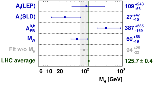
Figure 2 (right) shows the determination of $M_{H}$ in fits in which among the four observables providing the strongest constraint on $M_{H}$, namely $A_{l}$(LEP), $A_{l}$(SLD), $A_{\rm FB}^{0}$, and $M_{W}$, only the one indicated in a given row of the plot is included in the fit. For comparison also the indirect fit result (without the $M_{H}$ measurement) and the direct measurement are shown as vertical bands.

Figure 3: $\Delta\chi^{2}$ profiles as a function of the Higgs mass (top left), the top quark mass (top right), the $W$ boson mass (bottom left) and the effective weak mixing angle (bottom right). The data points placed along $\Delta\chi^{2}=1$ represent direct measurements of the respective observable and their $\pm 1\sigma$ uncertainties. The grey (blue) bands show the results when excluding (including) the new $M_{H}$ measurements from (in) the fits. For the blue bands as a function of $m_{t}$, $M_{W}$ and $\sin\!^{2}\theta^{\ell}_{{\rm eff}}$ the direct measurements of the observable have been excluded from the fit in addition (indirect determination). The solid black curves in the lower plots represent the SM prediction for $\sin\!^{2}\theta^{\ell}_{{\rm eff}}$ and $M_{W}$ derived from the minimal set of input measurements, as described in the text. In all figures the solid (dotted) lines illustrate the fit results including (ignoring) theoretical uncertainties in the fit.

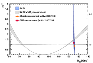
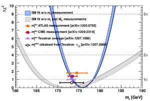
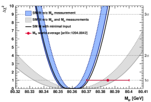
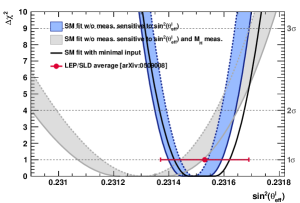
The remaining plots in Fig. 3 show the $\Delta\chi^{2}$ profile curves versus $m_{t}$ (top right), $M_{W}$ (bottom left), and $\sin\!^{2}\theta^{\ell}_{{\rm eff}}$ (bottom right) obtained without using the corresponding experimental measurement in the fit (indirect determination, cf. last column of Table 1). For comparison also the corresponding profile curves excluding in addition the new $M_{H}$ measurements are shown (grey bands). The results from the direct measurements for each variable are also indicated by data points at $\Delta\chi^{2}=1$. The insertion of $M_{H}$ substantially improves the precision of the fit predictions.

The fit indirectly determines the $W$ mass (cf. Fig. 3 – bottom left, blue band) to be

$$M_{W} = 80.3593\pm 0.0056_{m_{t}}\pm 0.0026_{M_{Z}}\pm 0.0018_{\Delta\alpha_{\rm had}}$$ (3)

$$\phantom{80.3593}\pm 0.0017_{\alpha_{\scriptscriptstyle S}}\pm 0.0002_{M_{H}}\pm 0.0040_{\rm theo}\,,$$

$$= 80.359\pm 0.011_{\rm tot}\;,$$ (4)

which exceeds the experimental world average in precision. The different uncertainty contributions originate from the uncertainties in the input values of the fit as given in the second column in Table 1. The dominant uncertainty is due to the top quark mass. Due to the weak, logarithmic dependence on $M_{H}$ the contribution from the uncertainty on the Higgs mass is very small compared to the other sources of uncertainty. Note that in the Rfit scheme [17, 18] the treatment of the theoretical uncertainty as uniform likelihood corresponds a linear addition of theoretical and experimental uncertainties. Quadratic addition would give a total uncertainty in the $M_{W}$ prediction of 0.008.

The indirect determination of the effective weak mixing angle (cf. Fig. 3 – bottom right, blue band) gives

$$\sin\!^{2}\theta^{\ell}_{{\rm eff}} = 0.231496\pm 0.000030_{m_{t}}\pm 0.000015_{M_{Z}}\pm 0.000035_{\Delta\alpha_{\rm had}}$$ (6)

$$\phantom{0.231496}\pm 0.000010_{\alpha_{\scriptscriptstyle S}}\pm 0.000002_{M_{H}}\pm 0.000047_{\rm theo}\,,$$

$$= 0.23150\pm 0.00010_{\rm tot}\;,$$ (7)

which is compatible and more precise than the average of the LEP/SLD measurements [9]. The total uncertainty is dominated by that from $\Delta\alpha_{\rm had}$ and $m_{t}$, while the contribution from the uncertainty in $M_{H}$ is again very small. Adding quadratically theoretical and experimantal uncertainties would lead to a total uncertainty in the $\sin\!^{2}\theta^{\ell}_{{\rm eff}}$ prediction of $0.00007$.

Finally, the top quark mass, cf. Fig. 3 (top right, blue band), is indirectly determined to be

$$m_{t}=175.8^{\>+2.7}_{\>-2.4}\>\mathrm{Ge\kern-1.00006ptV}\;,$$ (8)

in agreement with the direct measurement and cross-section based determination (cf. Footnote 5).

The measured value of $M_{H}$ together with the fermion masses, the strong coupling strength $\alpha_{\scriptscriptstyle S}(M_{Z}^{2})$ and the three parameters defining the electroweak sector and its radiative corrections (chosen here to be $M_{Z}$, $G_{F}$ and $\Delta\alpha_{\rm had}^{(5)}(M_{Z}^{2})$) form a minimal set of parameters allowing one, for the first time, to predict all the other SM parameters/observables. A fit using only this minimal set of input measurements yields the SM predictions $M_{W}=80.360\pm 0.011\>{\rm GeV}$ and $\sin\!^{2}\theta^{\ell}_{{\rm eff}}=0.23152\pm 0.00010$. The $\Delta\chi^{2}$ profile curves of these predictions are shown by the solid black lines in Fig. 3 (bottom left) and (bottom right). The agreement in central value and precision of these results with those from Eq. (4) and (7) (cf. blue bands in the plots) illustrates the marginal additional information provided by the other observables.

Figure 4: Contours of 68% and 95% CL obtained from scans of fixed $M_{W}$ and $m_{t}$. The blue (grey) areas illustrate the fit results when including (excluding) the new $M_{H}$ measurements. The direct measurements of $M_{W}$ and $m_{t}$ are always excluded in the fit. The vertical and horizontal bands (green) indicate the 1$\sigma$ regions of the direct measurements.

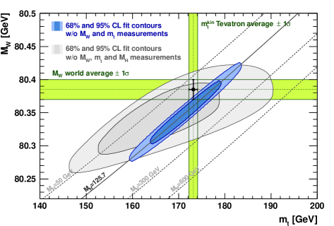
Figure 4 displays CL contours of scans with fixed values of $M_{W}$ and $m_{t}$, where the direct measurements of $M_{W}$ and $m_{t}$ were excluded from the fit. The contours show agreement between the direct measurements (green bands and data point), the fit results using all data except the $M_{W}$, $m_{t}$ and $M_{H}$ measurements (grey contour areas), and the fit results using all data except the experimental $M_{W}$ and $m_{t}$ measurements (blue contour areas). The observed agreement again demonstrates the impressive consistency of the SM.

Figure 5: Experimental constraints on the $S$ and $T$ parameters with respect to the SM reference ($M_{H,\rm ref}=126$ GeV and $m_{t,\rm ref}=173$ GeV). Shown are the 68%, 95% and 99% CL allowed regions, where the third parameter $U$ is left unconstrained (orange, left) or fixed to 0 (blue, right). The prediction in the SM is given by the black (grey) area when including (excluding) the new $M_{H}$ measurements.

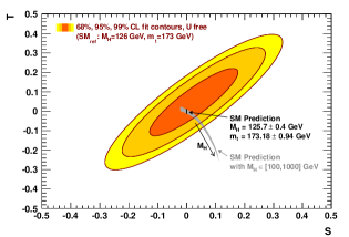
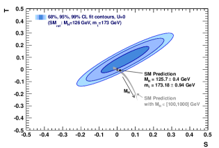
Following the approach in [6] we extract from the electroweak fit the $S,\,T,\,U$ parameters [35, 36] describing the difference between the oblique vacuum corrections as determined from the experimental data and the corrections expected in a reference SM (SM_ref defined by fixing $m_{t}$ and $M_{H}$). After the recent discovery, we change our definition of the reference SM for the $S,\,T,\,U$ calculation to $M_{H,\rm ref}=126$ GeV and $m_{t,\rm ref}=173$ GeV. With these we find:

$$S=0.03\pm 0.10\>,\hskip 14.22636ptT=0.05\pm 0.12\>,\hskip 14.22636ptU=0.03\pm 0.10\>,$$ (9)

with correlation coefficients of $+0.89$ between $S$ and $T$, and $-0.54$ ($-0.83$) between $S$ and $U$ ($T$ and $U$). Fixing $U=0$ we obtain $S|_{U=0}=0.05\pm 0.09$ and $T|_{U=0}=0.08\pm 0.07$ with a correlation coefficient of $+0.91$. Figure 5 shows the 68%, 95% and 99% CL allowed regions in the $(S,T)$ plane for freely varying $U$ (left) and the constraints found when fixing $U=0$ (right). For illustration also the SM prediction is shown. The $M_{H}$ measurement reduces the allowed SM area from the grey sickle, defined by letting $M_{H}$ float within the indicated range, to the narrow black strip.

4 Conclusion

Assuming the newly discovered particle at $\sim$126 $\mathrm{Ge\kern-1.00006ptV}$ to be the Standard Model (SM) Higgs boson, all fundamental parameters of the SM are known. It allows, for the first time, to overconstrain the SM at the electroweak scale and to evaluate its validity. The global fit to all the electroweak precision data and the measured Higgs mass results in a goodness-of-fit $p$-value of 0.07. Only a fraction of the contribution to the “incompatibility” stems from the Higgs mass, which agrees at the 1.3$\sigma$ level with the fit prediction. The largest deviation between the best fit result and the data is introduced by the known tension between $A_{\rm FB}^{0,b}$ from LEP and $A_{\ell}$ from SLD, predicting respectively a larger (by 2.5$\sigma$) and smaller (1.9$\sigma$) Higgs mass, and by $R^{0}_{b}$ for which an improved calculation increased the deviation from the measurement from previously 0.8$\sigma$ to 2.4$\sigma$.

The knowledge of the Higgs mass dramatically improves the SM predictions of several key observables. The uncertainties in the predictions of the $W$ mass, $\sin\!^{2}\theta^{\ell}_{{\rm eff}}$, and the top mass decrease from 28 to 11 $\mathrm{Me\kern-1.00006ptV}$, $2.3\cdot 10^{-5}$ to $1.0\cdot 10^{-5}$, and from 6.2 to 2.5 $\mathrm{Ge\kern-1.00006ptV}$, respectively. The improved accuracy sets a benchmark for direct measurements, which has been reached (and surpassed) only for the top mass. Theoretical uncertainties due to unknown higher order electroweak corrections contribute approximately half of the uncertainties in the $M_{W}$ and $\sin\!^{2}\theta^{\ell}_{{\rm eff}}$ predictions.

The results reported in this letter depend on the validity of the assumption that the observed particle is indeed the SM Higgs boson. New physics may lead to deviations in the couplings, which also affect the global fit. The next round of experimental updates by ATLAS and CMS will lead to a more precise assessment of the new particle’s properties and are expected with great excitement.

We thank Louis Fayard whose questions have triggered the more detailed error analysis for the $M_{W}$ and $\sin\!^{2}\theta^{\ell}_{{\rm eff}}$ predictions provided in this version of the paper.

References

- [1] ATLAS Collaboration, Phys. Lett. B (2012), [1207.7214].
- [2] CMS Collaboration, Phys. Lett. B (2012), [1207.7235].
- [3] ALEPH Collaboration, CDF Collaboration, D0 Collaboration, DELPHI Collaboration, L3 Collaboration, OPAL Collaboration, SLD Collaboration, LEP Electroweak Working Group, Tevatron Electroweak Working Group, SLD Electroweak and Heavy Flavour Groups, [1012.2367].
- [4] LEP Electroweak Working Group (LEP EWWG), http://lepewwg.web.cern.ch/LEPEWWG.
- [5] J. Erler and P. Langacker (in: Review for Particle Data Group), Phys. Rev. D86, 010001 (2012).
- [6] M. Baak et al., Eur. Phys. J. C72, 2003 (2012), [1107.0975].
- [7] H. Flacher et al., Eur. Phys. J. C60, 543 (2009), [0811.0009], Erratum-ibid. C71 (2011) 1718.
- [8] O. Eberhardt et al., [1209.1101].
- [9] The ALEPH, DELPHI, L3, OPAL, SLD Collaborations, the LEP Electroweak Working Group, the SLD Electroweak and Heavy Flavour Working Groups, Phys. Rept. 427, 257 (2006), [hep-ex/0509008].
- [10] CDF Collaboration, D0 Collaboration, T. E. W. Group, [1204.0042].
- [11] CDF Collaboration, D0 Collaboration, T. E. W. Group, [1003.2826].
- [12] CDF Collaboration, D0 Collaboration, T. Aaltonen et al., [1207.1069].
- [13] P. Skands and D. Wicke, Eur. Phys. J. C52, 133 (2007), [hep-ph/0703081].
- [14] D. Wicke and P. Z. Skands, Nuovo Cim. B123, S1 (2008), [0807.3248].
- [15] A. H. Hoang, A. Jain, I. Scimemi and I. W. Stewart, Phys. Rev. Lett. 101, 151602 (2008), [0803.4214].
- [16] A. H. Hoang and I. W. Stewart, Nucl. Phys. Proc. Suppl. 185, 220 (2008), [0808.0222].
- [17] A. Hoecker, H. Lacker, S. Laplace and F. Le Diberder, Eur. Phys. J. C21, 225 (2001), [hep-ph/0104062].
- [18] CKMfitter Group, J. Charles et al., Eur. Phys. J. C41, 1 (2005), [hep-ph/0406184].
- [19] M. Davier, A. Hoecker, B. Malaescu and Z. Zhang, Eur. Phys. J. C71, 1515 (2011), [1010.4180].
- [20] P. Baikov, K. Chetyrkin and J. H. Kuhn, Phys. Rev. Lett. 101, 012002 (2008), [0801.1821].
- [21] P. Baikov, K. Chetyrkin, J. Kuhn and J. Rittinger, Phys. Rev. Lett. 108, 222003 (2012), [1201.5804].
- [22] M. Awramik, M. Czakon, A. Freitas and G. Weiglein, Phys. Rev. D69, 053006 (2004), [hep-ph/0311148].
- [23] M. Awramik, M. Czakon and A. Freitas, JHEP 0611, 048 (2006), [hep-ph/0608099].
- [24] M. Awramik, M. Czakon, A. Freitas and G. Weiglein, Phys. Rev. Lett. 93, 201805 (2004), [hep-ph/0407317].
- [25] A. Freitas and Y.-C. Huang, JHEP 1208, 050 (2012), [1205.0299].
- [26] K. Hagiwara, S. Matsumoto, D. Haidt and C. Kim, Z. Phys. C64, 559 (1994), [hep-ph/9409380], Order of authors changed in journal.
- [27] K. Hagiwara, Ann. Rev. Nucl. Part. Sci. 48, 463 (1998).
- [28] G.-C. Cho and K. Hagiwara, Nucl. Phys. B574, 623 (2000), [hep-ph/9912260].
- [29] G.-C. Cho, K. Hagiwara, Y. Matsumoto and D. Nomura, JHEP 1111, 068 (2011), [1104.1769].
- [30] A. B. Arbuzov et al., Comput. Phys. Commun. 174, 728 (2006), [hep-ph/0507146].
- [31] D. Y. Bardin et al., Comput. Phys. Commun. 133, 229 (2001), [hep-ph/9908433].
- [32] S. Alekhin, A. Djouadi and S. Moch, Phys. Lett. B716, 214 (2012), [1207.0980].
- [33] ATLAS Collaboration, G. Aad et al., Eur.Phys.J. C72, 2046 (2012), [1203.5755].
- [34] CMS Collaboration, S. Chatrchyan et al., [1209.2319].
- [35] M. E. Peskin and T. Takeuchi, Phys. Rev. Lett. 65, 964 (1990).
- [36] M. E. Peskin and T. Takeuchi, Phys. Rev. D46, 381 (1992).